A resonance phenomenon for ground states of an elliptic equation of Emden–Fowler type

J. Differential Equations 198 (2004) 1–15

A resonance phenomenon for ground states of anelliptic equation of Emden–Fowler type

Isabel Flores

Departamento de Matematicas, Facultad de Ciencias Casilla 653 Correo 1, Universidad de Chile,

Santiago, Chile

Received August 15, 2000

Abstract

We consider the problem

Du þ up þ uq ¼ 0 in RN ; ð1Þ

0ouðxÞ-0 as jxj-þN; ð2Þ

where NX3; and

1opoN þ 2

N � 2oq: ð3Þ

Lin and Ni observed that if one further has q ¼ 2p21; then there exists an explicit radial

solution of (1)–(2) of the form uðrÞ ¼ ð ABþr2

Þ1

p�1: However, the question of existence in the

general range has remained basically open. We prove that if the range of p is further restricted

to

p >N þ 2

ffiffiffiffiffiffiffiffiffiffiffiffiffiN � 1

p

N þ 2ffiffiffiffiffiffiffiffiffiffiffiffiffiN � 1

p� 4

; ð4Þ

then for q ¼ 2p21 not only this explicit solution exists, but also an infinite number of radial

solutions with fast decay Oðr2�NÞ: If q is close to 2p21; a large number of such solutions still

persists. This phenomenon will actually take place whenever (3) and (4) hold and a slow decay

solution exists. A similar assertion holds if instead of (4) we assume Np10 or qo N�2ffiffiffiffiffiffiffiffiN�1

p

N�2ffiffiffiffiffiffiffiffiN�1

p�4;

and that a radial singular solution of (1)–(2) exists.

r 2002 Elsevier Inc. All rights reserved.

ARTICLE IN PRESS

E-mail address: [email protected], [email protected] (I. Flores).

0022-0396/02/$ - see front matter r 2002 Elsevier Inc. All rights reserved.

PII: S 0 0 2 2 - 0 3 9 6 ( 0 2 ) 0 0 0 1 5 - 3

1. Introduction

A classical nonlinear elliptic partial differential equation is the so-called Emden–Fowler equation

Du þ up ¼ 0 ð1:1Þ

in RN ; where p > 1; NX1; and D denotes the standard Laplacian operator. As inmany semilinear elliptic equations arising in applications, a basic question is that offinding ground states, namely positive solutions defined in the entire space which tendto zero as jxj-N: The above equation was introduced by Lane in the mid-19thcentury, as a model of the distribution of clusters of stars in Astrophysics. It was in1931 that Fowler [6] solved completely the problem of finding radially symmetricequations u ¼ uðjxjÞ: The introduction of the ingenious transformation

xðtÞ ¼ r2

p�1uðrÞjr¼et

actually reduces the equation to an autonomous second-order ordinary differentialequation whose trajectories can be fully understood via standard phase-planeanalysis (see also, for instance, the appendix in [10]). As it is well known, when NX3

the critical exponent p ¼ Nþ2N�2

sets a dramatic shift in the structure of the radial

solutions of this equation. For instance if 1opoNþ2N�2

; no positive solution of (1.1)

defined in the entire space exists. On the other hand, if p ¼ Nþ2N�2; such solutions exist

and are all of the form

ulðrÞ ¼ aNl

l2 þ r2

� �N�22; r ¼ jxj; l > 0:

When p > Nþ2N�2

; ground states also exist and they are constituted by a continuum of

the form ulðrÞ ¼ l2

p�1vðlrÞ: There is also a difference in asymptotic behavior of the

ground states between the critical and supercritical cases. In fact, for p ¼ Nþ2N�2

ulðrÞBaNlN�22 r�ðN�2Þ

as r-þN; while for p > Nþ2N�2

ulðrÞBCp;Nr�2

p�1;

where the constant Cp;N ¼ ð 2p�1

f 2p�1

� ðN � 2ÞgÞ1

p�1 is precisely that making the right-

hand side of the above relation a (singular) solution of the equation. Observe that

this singular solution still exists when p ¼ Nþ2N�2

but its decay rate is slower than that of

ARTICLE IN PRESSI. Flores / J. Differential Equations 198 (2004) 1–152

the ground states: like r�N�22 : It is worthwhile mentioning that if ppNþ2

N�2; all possible

positive solutions are known to be radially symmetric around some point [5,7].In view of the above discussion, it seems natural to consider now the problem of

finding positive solutions to the following semilinear elliptic equation in RN :

Du þ up þ uq ¼ 0; ð1:2Þ

0ouðxÞ-0 as jxj-þN: ð1:3Þ

A question that has remained open for some time is that of whether there exist

positive, say, radially symmetric solutions to this problem RN ; NX3 when p and q

are, respectively, sub and supercritical, namely

1opoN þ 2

N � 2oq: ð1:4Þ

It is known that in this range all solutions to (1.2)–(1.3) need to be radially symmetricaround some point, as established by Zou in [13]. An interesting example wasdiscovered by Lin and Ni in [11]. If p and q lie in the range (1.4) and additionally oneassumes q ¼ 2p � 1; then there is a solution of the form

uðrÞ ¼ A

B þ r2

� � 1p�1

;

where A and B are explicit positive constants depending on p and N: For radialsolutions of (1.2)–(1.3), one can show that their behavior as r ¼ xj j-þN may only

be of one of the following two types: either Oðr�ðN�2ÞÞ in whose case we say that the

solution is of fast decay, or BCp;Nr�2

p�1; which we call slow decay.

The recent works [1,2] have partly answered the existence problem through the

following asymptotic result: If one fixes NN�2

opoNþ2N�2

; and sets q ¼ Nþ2N�2

þ e; thenthere exists a sequence ekk0 such that if 0oeoek; k ¼ 1; 2;y; then (1.2)–(1.3) haveat least k radial solutions with fast decay. A similar situation occurs if one now fixes

q > Nþ2N�2

and sets p ¼ Nþ2N�2

� e:We observe that Lin and Ni’s solution is actually of slow decay; so it is not one

covered by the above asymptotic result. We observe also that this existence resultleaves out in principle the case q ¼ 2p21: On the other hand, the presence of slow-decay solutions is not expected to be generic, as discussed in [2]. It is also a relativelysimple matter to establish uniqueness of a radially symmetric slow-decay solution to(1.2)–(1.3) in case that it exists. A similar fact is valid for singular solutions: a

positive radially symmetric solution uðjxjÞ of (1.2) in RN\f0g is called a radial

singular ground state of (1.2) if uðrÞ-þN as r-0:Our primary purpose in this work is to reveal a rather striking resonance

phenomenon that arises when q ¼ 2p � 1 if the range of p is a bit further restricted.

ARTICLE IN PRESSI. Flores / J. Differential Equations 198 (2004) 1–15 3

Not only Lin and Ni’s solution exists, but also infinitely many solutions with fast

decay. Moreover, if we fix p; then for all q sufficiently close to 2p � 1; one has anarbitrarily large number of solutions.

In what follows, we will always assume that p and q lie in the range

N

N � 2opo

N þ 2

N � 2oq: ð1:5Þ

Theorem 1.1. Assume that p and q satisfy (1.5) and additionally that


p


p� 4

op: ð1:6Þ

Then, given any integer kX1; there exists a number ek > 0 such that

if jq � ð2p � 1Þj oek then there are at least k radial positive ground states with fast

decay of (1.2)–(1.3). In particular, if q ¼ 2p � 1; then there exist infinitely many

ground states.

This result is a direct consequence of a more general fact which we state below.

Theorem 1.2 (a). Assume that p and q satisfy (1.5) and that (1.6) holds. Then if there is

a radial ground state of (1.2)–(1.3) with slow decay, there are infinitely many radial

ground states with fast decay.

(b) Assume that

Np10 or qoN � 2


p

N � 2ffiffiffiffiffiffiffiffiffiffiffiffiffiN � 1

p� 4

: ð1:7Þ

Then if there is a singular radial ground state of (1.2), there are infinitely many radial

ground states with fast decay.

(c) If %p; %q are numbers like in cases (a) or (b), then given any integer kX1; there

exists a number ek > 0 such that if

jp � %pj þ jq � %qjoek;

then (1.2)–(1.3) has at least k radial solutions with fast decay.

We remark that besides the slow-decay ground state in Lin and Ni’s example, it is

established in [2] that for fixed q > Nþ2N�2

there is a sequence p ¼ pkmNþ2N�2

; along which a

radial singular ground state exists. Symmetrically, if NN�2

opoNþ2N�2

is fixed, then there

is a sequence q ¼ qkkNþ2N�2

along which a slow decay radial ground state, singular or

non-singular exists.


2. Preliminaries: the set-up

We search for positive radially symmetric solutions u ¼ uðrÞ; r ¼ jxj; of (1.2)–(1.3), namely solutions of the ordinary differential equation

u00 þ N � 1

ru0 þ u

pþ þ u

qþ ¼ 0; r > 0; ð2:1Þ

u0ð0Þ ¼ 0; 0ouðrÞ-0 as r-þN: ð2:2Þ

Here we have denoted uþ ¼ maxfu; 0g:We consider the classical Emden–Fowler transformation

xðtÞ ¼ r2

p�1uðrÞjr¼et ð2:3Þ

which recasts Eq. (2.1) into the equivalent problem

x00 � ax0 þ xpþ þ e�gtx

qþ � bx ¼ 0; �NotoþN: ð2:4Þ

where

a ¼ 4

p � 1� ðN � 2Þ; b ¼ 2

p � 1N � 2� 2

p � 1

� �; g ¼ 2

q � p

p � 1:

Standard calculations show that finding a positive solution of (2.1)–(2.2) isequivalent to finding a positive solution xðtÞ in R of (2.4) such that

xðtÞ-0 as t-7N:

Introducing the variables y ¼ x0 and z ¼ e�gt; Eq. (2.4) becomes equivalent to theautonomous first-order system

x0 ¼ y;

y0 ¼ ay þ bx � xpþ � zx

qþ;

z0 ¼ �gz;

zX0:

8>>><>>>:

ð2:5Þ

The plane z ¼ 0 is invariant under the flow associated to system (2.5); we thus restrictourselves to analyze trajectories that lie in the half-space zX0: Then plane z ¼ 0

contains the two singularities of the flow ON ¼ ð0; 0; 0Þ and PN ¼ ðb1

p�1; 0; 0Þ whichare hyperbolic. Moreover, if

p >N þ 2


p


p� 4

; ð2:6Þ


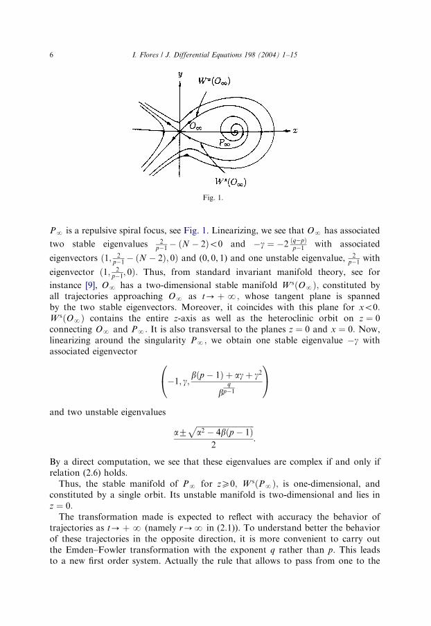
PN is a repulsive spiral focus, see Fig. 1. Linearizing, we see that ON has associated

two stable eigenvalues 2p�1

� ðN � 2Þo0 and �g ¼ �2ðq�pÞp�1

with associated

eigenvectors ð1; 2p�1

� ðN � 2Þ; 0Þ and (0, 0, 1) and one unstable eigenvalue, 2p�1

with

eigenvector ð1; 2p�1

; 0Þ: Thus, from standard invariant manifold theory, see for

instance [9], ON has a two-dimensional stable manifold W sðONÞ; constituted byall trajectories approaching ON as t-þN; whose tangent plane is spannedby the two stable eigenvectors. Moreover, it coincides with this plane for xo0:W sðONÞ contains the entire z-axis as well as the heteroclinic orbit on z ¼ 0connecting ON and PN: It is also transversal to the planes z ¼ 0 and x ¼ 0: Now,linearizing around the singularity PN; we obtain one stable eigenvalue �g withassociated eigenvector

�1; g;bðp � 1Þ þ agþ g2

bq

p�1

0@

1A

and two unstable eigenvalues

a7ffiffiffiffiffiffiffiffiffiffiffiffiffiffiffiffiffiffiffiffiffiffiffiffiffiffiffiffiffiffia2 � 4bðp � 1Þ

p2

:

By a direct computation, we see that these eigenvalues are complex if and only ifrelation (2.6) holds.

Thus, the stable manifold of PN for zX0; W sðPNÞ; is one-dimensional, andconstituted by a single orbit. Its unstable manifold is two-dimensional and lies inz ¼ 0:

The transformation made is expected to reflect with accuracy the behavior oftrajectories as t-þN (namely r-N in (2.1)). To understand better the behaviorof these trajectories in the opposite direction, it is more convenient to carry outthe Emden–Fowler transformation with the exponent q rather than p: This leadsto a new first order system. Actually the rule that allows to pass from one to the

ARTICLE IN PRESS

Fig. 1.

I. Flores / J. Differential Equations 198 (2004) 1–156

other is

x ¼ xz1

q�1; y ¼ y � gx

q � 1

� �z

1q�1; z ¼ 1

zp�1q�1

: ð2:7Þ

Then ðx; y; zÞ satisfies the system

x0 ¼ y;

y0 ¼ �*ay þ *bx � xqþ � zx

pþ

z0 ¼ *gz;

8><>: ; ð2:8Þ

where now

a ¼ ðN � 2Þ � 4

q � 1; *b ¼ 2

q � 1N � 2� 2

q � 1

� �; *g ¼ 2

q � p

q � 1:

Similarly as before, the plane z ¼ 0 is invariant under this new flow whose

singularities are the points O0 ¼ ð0; 0; 0Þ and P0 ¼ ð *b1

q�1; 0; 0Þ; which are againhyperbolic. For the flow restricted to z ¼ 0; O0 is a hyperbolic saddle and P0 is ahyperbolic attractor which are connected by a heteroclinic orbit, see Fig. 2.

Linearizing the flow around O0; one obtains one stable eigenvalue 2q�1�

ðN � 2Þo0 with associated eigenvector ð1; 2q�1

� ðN � 2Þ; 0Þ and two unstable

eigenvalues 2q�1

and *g ¼ 2 ðq�pÞq�1

with associated eigenvectors ð1; 2q�1

; 0Þ and (0, 0, 1).

Thus, O0 has a two-dimensional unstable manifold WuðO0Þ; constituted by alltrajectories approaching O0 as t-�N; whose tangent plane is spannedby the two unstable eigenvectors and it coincides with this plane for xo0:WuðO0Þcontains the entire z-axis as well as the heteroclinic orbit on z ¼ 0 connect-ing O0 and P0: It is also transversal to the planes z ¼ 0 and x ¼ 0: Now,linearizing around the singularity P0; we obtain one unstable eigenvalue *g with

ARTICLE IN PRESS

Fig. 2.

I. Flores / J. Differential Equations 198 (2004) 1–15 7

associated eigenvector

�1;�*g;*bðq � 1Þ þ *a*gþ *g2

*bp

q�1

0@

1A

and two stable eigenvalues

�*a7ffiffiffiffiffiffiffiffiffiffiffiffiffiffiffiffiffiffiffiffiffiffiffiffiffiffiffiffiffiffi*a2 � 4 *bðq � 1Þ

q2

:

Let us observe that these eigenvalues are complex if and only if

Np10 or qoN � 2


p

N � 2ffiffiffiffiffiffiffiffiffiffiffiffiffiN � 1

p� 4

ð2:9Þ

and the stable manifold is two-dimensional and lies in z ¼ 0: Restricted to this plane,P0 is a spiral attracting focus, see Fig. 1. Its unstable manifold WuðP0Þ in z > 0 isone-dimensional, and constituted by a single orbit.

The next result further clarifies the picture of the phase space, see Fig. 3.

Lemma 2.1. The unstable manifold of P0; WuðP0Þ is contained in the closure of the

unstable manifold of O0; WuðO0Þ: Similarly, the stable manifold of PN; W sðPNÞ is

contained in the closure of the stable manifold of ON; WsðONÞ:

We postpone the proof of this for the appendix.We say that two system x0 ¼ f ðxÞ and y0 ¼ gðyÞ with respective singularities P0

and Q0 are C1-equivalent around these points, if there is a C1-diffeomorphismbetween respective neighborhoods of these points which transforms trajectories ofthe first system into trajectories of the other, preserving orientations. The followingfact will be important for our purposes.

Lemma 2.2. System (2.5) is C1-equivalent to its linearized system around PN: So is

system (2.8) around P0, provided that relation (2.9) holds. Moreover, the associated

diffeomorphisms preserve orientation.

We also leave this result for the appendix, and we go onto the proof of Theorem 1.2.

3. The proof of the main results

We want to find fast decay solutions to (1.2)–(1.3). At the level of thetransformation x given by (2.3), this corresponds to a trajectory attracted byON as t-N; namely it must lie in W sðONÞ: On the other hand, at the level ofsystem (2.8), it must approach O0 as t-�N; hence it lies also in the manifold


WuðO0Þ: Hence our task is to show that under the conditions of Theorem 1.2, parts(a) and (b), there are infinitely many distinct trajectories lying simultaneously in bothtwo-dimensional manifold. We observe that such a trajectory must remain positivein its x-coordinate. In fact, a trajectory in WuðO0Þ which crosses the plane x ¼ 0must do it transversally and after it never comes back to the positive side. Similarlyfor a trajectory in W sðONÞ: The strategy to establish this is as follows: we stand on aneighborhood of PN and prove that the curves corresponding to the intersection ofthese manifolds with z ¼ z0; very small z0; actually intersect infinitely many times,thus giving rise to infinitely many of the seeked trajectories.

We prove first the assertion of part (a). From Lemma 2.2, we know that in the

situation here considered, the flow (2.5) is C1-equivalent in a neighborhood of PN tothe following linear flow:

%x0 ¼ %y;

%y0 ¼ a %x þ b %y þ c%z;

%z0 ¼ dz;

8><>: ð3:1Þ

ARTICLE IN PRESS

Fig. 3.


where

a ¼ bð1� pÞ; b ¼ a; c ¼ �bq

p�1; d ¼ �g:

After a suitable linear transformation we, immediately check that this system is also

C1-equivalent to

%x0 ¼ %y;

%y0 ¼ a %x þ b %y;

%z0 ¼ dz:

8><>: ð3:2Þ

Let F : V-U be the diffeomorphism setting the equivalence between (2.5) and (3.2),where V is a neighborhood of PN and U one of O: As in the original system (2.5),the origin in (3.2) is a repelling focus when the flow is restricted to the plane %z ¼ 0and the %z-axis is its corresponding stable manifold.

Let us recall that stable manifold of ON contains the stable manifold of PN in itsclosure; hence in the neighborhood V of PN where the equivalence is valid, there isan invariant manifold, namely W sðONÞ-V: To this manifold, it correspondsthrough the equivalence F; an invariant manifold M of system (3.2) inside U: LetcðtÞ be the image through F restricted to z ¼ 0gf -V; of an orbit corresponding tothe heteroclinic trajectory which connects PN and ON: It is easily checked, aftermaking U and V smaller if necessary, that the manifold M must be constitutedexactly by the set of points of the form ðcðtÞ; %zÞ which lie inside U; the neighborhoodof O; see Fig. 4.

Let xðtÞ be the solution of (2.5) which corresponds to a slowly decaying solution of(2.1)–(2.2), which exists by hypothesis. Clearly this trajectory corresponds preciselyto the (one-dimensional) stable manifold of PN; hence its image through F for allsufficiently large t is precisely the part of the %z-axis inside U: It of course lies also inWuðO0Þ (described in the coordinates (x; y; z) via the inverse of transformation(2.7)).

Let us consider a small z0 so that the plane z ¼ z0 intersects V: Let us consideralso the image of WuðO0Þ through the equivalence F; near PN: This two-dimensional manifold lies on a transversal section to the linear flow of (3.2), given byS ¼ FðV-fz ¼ z0gÞ: Now let us consider the transition map which goes from S tothe plane %z ¼ d with a sufficiently small d: Summarizing, we have a function H

defined on V-fz ¼ z0g with values in U-f%z ¼ dg where H is the composition of Fand the transition map. We observe that H is a C1-diffeomorphism. Sincetrajectories cross transversally the plane z ¼ z0; so does WuðO0Þ: Hence

WuðO0Þ-fz ¼ z0g defines a C1 curve, except possibly at its endpoint, whichcorresponds to

fP1g ¼ WuðP0Þ-fz ¼ z0g:

Since H is a diffeomorphism, it follows that the set HðWuðO0Þ-V-fz ¼ z0gÞ is aC1 curve, which we call g inside the planar section U-f%z ¼ dg which contains thepoint P2 ¼ ð0; 0; dÞ: Note that P2aHðP1Þ since P1 is not in WuðO0Þ:


Let us recall that the image through the equivalence of W sðONÞ intersected withU-f%z ¼ dg is precisely the curve sðtÞ ¼ ðcðtÞ; dÞ; a spiral around the point P ¼ð0; 0; dÞ; which can be explicitly computed. Summarizing, we need to show that the

spiral curve s around P and the C1 curve g; which contains the point P in its interior,do intersect. Each intersection will correspond to a trajectory in WuðO0Þ-W sðONÞ:It follows from Lemma 4.1 in the appendix (the case yð0þÞ finite) that these curvesmust indeed intersect infinite times, each of which gives rise to infinitely manydistinct solutions of (1.2)–(1.3), see Fig. 5.

Now, the remark after Lemma 4.1 and the continuity under parameters of thesolutions of the system, implies that if p and q are slightly perturbed, a large numberof these intersections will persist. This proves the assertion of part (c) of the theoremin case that the conditions of part (a) hold.

Let us now consider the case of part (b). In case that (1.7) holds, and there exists asingular solution with fast decay, the proof is symmetric to the one above.

Thus we assume that there is a singular solution with slow decay (a verydegenerate case, which we cannot a priori discard) and that (1.7) holds. This meansthat the unstable manifold of P0 coincides with the stable manifold of PN: We

ARTICLE IN PRESS

Fig. 5.

Fig. 4.


consider a function H defined similarly as in the proof of part (a), except that nowthe endpoint of the curve g is assumed to coincide with (0, 0, d). The stable eignvaluesof P0 are complex, so the curve gamma is a spiral. In fact, this follows again from the

C1-equivalence orientation preserving with the lineralization around P0; in aneighborhood of these point, which implies this character in a section z ¼ d; a smalld: Then the flow lifts this section diffeomorphically towards z ¼ þN; namely toz ¼ 0�: If the unstable eigenvalues of PN are complex, then as before thecorresponding curve s is a spiral. Both spirals have the same endpoint; theyhowever wind in opposite directions, as it is easily argued, see Fig. 6. In such a case,

Lemma 4.1 for yð0þÞ ¼ �N now applies. If the eigenvalues of PN turned out to be

real, s would not be a spiral but a C1 curve up to its endpoint. This is again a

consequence of C1-equivalence with the linearization, as stated in Lemma 2.2. Thissituation makes again Lemma 4.1 applicable.

Finally the remaining part of assertion (c) follows again from the remark afterLemma 4.1. This concludes the proof of the theorem. &

Appendix

First we prove the topological facts used in the proof of the theorem, which areincluded in Lemma 4.1 below. Let P0 be a point in the plane. We consider a spiralcurve s around P0 of the following form:

sðtÞ ¼ P0 þ rðtÞeimðtÞ; tA½0;NÞ:

We assume r and m are continuous, that 0orðtÞorð0Þ for t > 0; thatrðtÞ-0 as t-N; and also that mð0Þ ¼ 0pmðtÞ with mðtÞ-0 as t-N: Letnow gðsÞ; sAð0; 1� be a continuous curve of the form

gðsÞ ¼ P0 þ rðsÞeiyðsÞ; sAð0; 1�

with rðsÞ > 0; yðsÞ continuous functions in (0,1] such that rð0þÞ ¼ 0: yðsÞ satisfies

that either yð0þÞ ¼ y0; a finite number, or yð0þÞ ¼ �N: We also assume that both sand g do not have self-intersections.

We have the validity of the following fact.

ARTICLE IN PRESS

Fig. 6.

I. Flores / J. Differential Equations 198 (2004) 1–1512

Lemma 4.1. Let s and g be curves as above. Assume additionally that rðsÞorð0Þ for all

tA½0; 1� and that gð1ÞaP0 and does not lie on the curve s. Then the curves g and sintersect an infinite number of times.

Proof. We lift the curves g and s to the universal covering of the plane without P0;the polar coordinates plane around P0;ðr; yÞ; r > 0; yAR: Then the lifting of s is of

course given by

*sðtÞ ¼ ðrðtÞ; mðtÞÞ

and that of g by *gðsÞ ¼ ðrðsÞ; yðsÞÞ: From the assumptions made, Jordan’s theoremimplies that the curve *g separates the strip ð0; rð0Þ� R of the r2y plane into twocomponents A� and Aþ to the ‘‘left’’ and to the ‘‘right’’ of the curve g; respectively.Also, the curve *g lies entirely inside this strip. Consider the family of translates*gk ¼ *gþ ð0; 2kpÞ; which are also liftings of g: Given a number n; consider a tn suchthat mðtÞ > mðtnÞ; rðtÞo1=n for all t > tn: The curve s splits again the part of the An

strip with y > mðtnÞ into two components A�n and Aþ

n : If yð0þÞ ¼ y0 is finite, we

extend *g with half of the y-axis to the left of yð0Þ: Then, if k is chosen sufficientlylarge, the following happens: there are points of *gk which lie on A�

n ; while necessarily

*gkð1Þ lies on Aþn : It follows by connectedness that the curve *gk intersects *s somewhere

in An: Since the r-coordinate of this point is less than 1n; and n is arbitrary; this

inherits infinitely many intersections of the original curve g and s; as desired. &

Remark. The topological nature of the above argument yields its ‘‘stability’’ in thefollowing sense: There exist numbers ek; sk; tk such that for any continuous curvess1ðtÞ; tAð0;N� and g1ðsÞ; sAð0; 1� such that

js1ðtÞ � sðtÞj þ jg1ðsÞ � gðsÞjoek

for all, tAð0; tk�; sA½sk; 1�; there are at least k distinct intersection points of thecurves s1 and g1:

Proof of Lemma 2.1. For the proof of this result, we will make use of the well-known Palis’ l-lemma, see for instance [8] or [12]. Its statement in the context we aredealing with is as follows.

Lemma 4.2. Consider a system of the form x0 ¼ f ðxÞ; f of class C1 in aneighborhood V of a hyperbolic singularity P: Let Xt denote its associated flow.Let us consider the (local) stable and unstable manifolds W sðPÞ; WuðPÞ; withrespective dimensions ns and nu: Let D be an nu dimensional disk which intersectstransversally W sðPÞ and contains a point Q of W sðQÞ: Let Bu be any disk insideWuðQÞ which contains Q: Let Dt be the connected component of XtðDÞ-V which

contains XtðQÞ: Then, given e > 0; there exists a t0 > 0 such that Dt is C1 e-close toBu for all t > t0: In particular, given any point Q1AB; there is a point in Dt which isat a distance less than e from Q0:


As we have seen, P0 is a hyperbolic singularity whose unstable manifold WuðP0Þ isa one-dimensional curve, and W sðP0Þ two-dimensional. Take a short segmenttransversal to the z ¼ 0 plane which lies entirely in the two-dimensional manifoldWuð00Þ (taken for instance close and almost parallel to the z-axis). By virtue of theabove lemma, the flow will take this segment into a one-dimensional segment, stillcontained in WuðO0Þ; which gets arbitrarily uniformly close to any given finite pieceof the curve WuðP0Þ: This proves that WuðP0Þ lies on the boundary of WuðO0Þ:The symmetric assertion that W sðPNÞ is contained in the boundary of W sðONÞfollows similarly. &

Proof of Lemma 2.2. To this end, we employ the following result, due toBelitskij [3,4].

Lemma 4.3. Suppose we have a system of the form x0 ¼ f ðxÞ with f ðx0Þ ¼ 0 and f

smooth in a neighborhood of x0: Assume also that x0 is a hyperbolic saddle of f with

eigenvalues l1;y; ln: Assume also that none of the relations Re li ¼ Re lj þ Re lk is

fulfilled. Then the system is C1-equivalent in a neighborhood of x0 to its linear part, in

the sense that there is a C1 diffeomorphism F from a neighborhood of x0 onto a

neighborhood of 0, with Fðx0Þ ¼ 0 which takes trajectories of the system x0 ¼ f ðxÞ into

trajectories of the linear system y0 ¼ f 0ðx0Þy; preserving orientation.

This result applies immediately to system (2.5) around PN if the unstableeigenvalues are not real, since we have two eigenvalues with the same, negative realparts, and a third eigenvalue which is positive. Then none of the relations Re li ¼Re lj þ Re lk is possible. The same happens in system (2.8) around P0 if its stable

eigenvalues are not real. If the unstable eigenvalues of PN are real, then we see thatthe only possibility to have one of these combinations is that

�gþ aþffiffiffiffiffiffiffiffiffiffiffiffiffiffiffiffiffiffiffiffiffiffiffiffiffiffiffiffiffiffia2 � 4bðp � 1Þ

p2

¼ a�ffiffiffiffiffiffiffiffiffiffiffiffiffiffiffiffiffiffiffiffiffiffiffiffiffiffiffiffiffiffia2 � 4bðp � 1Þ

p2

;

namely

g ¼ffiffiffiffiffiffiffiffiffiffiffiffiffiffiffiffiffiffiffiffiffiffiffiffiffiffiffiffiffiffia2 � 4bðp � 1Þ

q:

But this is impossible since g > a; as immediately checked from the definitions ofthese numbers. &

Acknowledgments

I would like to thank Rodrigo Bamon and Manuel del Pino, for usefulconversations and suggestions in the preparation of this paper. This work has beenpartly supported by FONDECYT postdoctoral grant 301-0044.


References

[1] R. Bamon, I. Flores, M. del Pino, Positive solutions of elliptic equations in RN with a super-

subcritical nonlinearity, C.R. Acad. Sci. Paris 330 (2000) 187–191.

[2] R. Bamon, I. Flores, M. del Pino, Ground states of semilinear elliptic equations: a geometric

approach, Ann. Inst. H. Poincare Anal. Non Lineaire, in preparation.

[3] G.R. Belitskij, Equivalence and normal forms of germs of smooth mappings, Russ. Math. Surv. 33

(1978) 101–177.

[4] G.R. Belitskij, Normal Forms, Invariants and Local Mappings, Naukova Dumka, Kiev, 1979, p. 176.

[5] L. Caffarelli, B. Gidas, J. Spruck, Asymptotic symmetry and local behavior of semilinear elliptic

equations with critical Sobolev growth, Comm. Pure Appl. Math. 42 (3) (1989) 271–297.

[6] R. Fowler, Further studies of Emden’s and similar differential equations, Quart. J. Math. 2 (1931)

259–288.

[7] B. Gidas, J. Spruck, Global and local behavior of positive solutions of nonlinear elliptic equations,

Comm. Pure Appl. Math. 34 (1981) 525–598.

[8] J. Guckenheimer, P. Holmes, Nonlinear Oscillations, Dynamical Systems and Bifurcations of Vector

Fields, Springer, New York, 1983.

[9] M. Hirsch, C. Pugh, M. Schub, Invariant Manifolds, Lecture Notes in Mathematics, Vol. 583,

Springer, New York, 1977.

[10] R. Johnson, X. Pan, Y. Yi, Positive solutions of super-critical elliptic equations and asymptotics,

Comm. Partial Differential Equations 18 (1993) 977–1019.

[11] C.-S. Lin, W.-M. Ni, A counterexample to the nodal line conjecture and a related semilinear

equation, Proc. Amer. Math. Soc. 102 (2) (1988) 271–277.

[12] J. Palis, W. de Melo, Geometric Theory of Dynamical Systems: An Introduction, Springer, New

York, Heidelberg, Berlin, 1982.

[13] H. Zou, Symmetry of ground states of semilinear elliptic equations with mixed Sobolev growth,

Indiana Univ. Math. J. 45 (1996) 221–240.


Documents

A resonance phenomenon for ground states of an elliptic equation of Emden–Fowler type