Embed Size (px)
Citation preview

HAL Id: tel-02397287https://tel.archives-ouvertes.fr/tel-02397287
Submitted on 6 Dec 2019
HAL is a multi-disciplinary open accessarchive for the deposit and dissemination of sci-entific research documents, whether they are pub-lished or not. The documents may come fromteaching and research institutions in France orabroad, or from public or private research centers.
L’archive ouverte pluridisciplinaire HAL, estdestinée au dépôt et à la diffusion de documentsscientifiques de niveau recherche, publiés ou non,émanant des établissements d’enseignement et derecherche français ou étrangers, des laboratoirespublics ou privés.
A random matrix framework for large dimensionalmachine learning and neural networks
Zhenyu Liao
To cite this version:Zhenyu Liao. A random matrix framework for large dimensional machine learning and neural networks.Other. Université Paris-Saclay, 2019. English. NNT : 2019SACLC068. tel-02397287

Thes
ede
doct
orat
NN
T:2
019S
AC
LC06
8
Theorie des matrices aleatoires pourl’apprentissage automatique en grandedimension et les reseaux de neurones
These de doctorat de l’Universite Paris-Saclaypreparee a CentraleSupelec
Ecole doctorale n580 Sciences et Technologies de l’Information et de laCommunication (STIC)
Specialite de doctorat : Mathematiques et Informatique
These presentee et soutenue a Gif-sur-Yvette, le 30/09/2019, par
M. ZHENYU LIAO
Composition du Jury :
M. Eric MoulinesProfesseur, Ecole Polytechnique President
M. Julien MairalDirecteur de recherche (INRIA), Grenoble Rapporteur
M. Stephane MallatProfesseur, ENS Paris Rapporteur
M. Arnak DalalyanProfesseur, ENSAE Examinateur
M. Jakob HoydisDocteur, ingenieur de recherche, Nokia Bell Labs Saclay Examinateur
Mme. Mylene MaidaProfesseure, Universite de Lille Examinateur
M. Michal ValkoCharge de recherche (INRIA), Lille Examinateur
M. Romain CouilletProfesseur, CentraleSupelec Directeur de these
M. Yacine ChitourProfesseur, Universite Paris-Sud Co-directeur de these

UNIVERSITY PARIS-SACLAY
DOCTORAL THESIS
A Random Matrix Framework forLarge Dimensional Machine Learning
and Neural Networks
Author:Zhenyu LIAO
Supervisor:Romain COUILLET
Yacine CHITOUR
A thesis submitted in fulfillment of the requirementsfor the degree of Doctor of Philosophy
in the
Laboratoire des Signaux et SystèmesSciences et technologies de l’information et de la communication (STIC)
October 15, 2019

ii

Contents
List of Symbols v
Acknowledgments vii
1 Introduction 11.1 Motivation: the Pitfalls of Large Dimensional Statistics . . . . . . . . . . . 2
1.1.1 Sample covariance matrices in the large n, p regime . . . . . . . . . 31.1.2 Kernel matrices of large dimensional data . . . . . . . . . . . . . . . 61.1.3 Summary of Section 1.1 . . . . . . . . . . . . . . . . . . . . . . . . . 10
1.2 Random Kernels, Random Neural Networks and Beyond . . . . . . . . . . 111.2.1 Random matrix consideration of large kernel matrices . . . . . . . 131.2.2 Random neural networks . . . . . . . . . . . . . . . . . . . . . . . . 201.2.3 Beyond the square loss: the empirical risk minimization framework 231.2.4 Summary of Section 1.2 . . . . . . . . . . . . . . . . . . . . . . . . . 25
1.3 Training Neural Networks with Gradient Descent . . . . . . . . . . . . . . 261.3.1 A random matrix viewpoint . . . . . . . . . . . . . . . . . . . . . . . 271.3.2 A geometric approach . . . . . . . . . . . . . . . . . . . . . . . . . . 281.3.3 Summary of Section 1.3 . . . . . . . . . . . . . . . . . . . . . . . . . 33
1.4 Outline and Contributions . . . . . . . . . . . . . . . . . . . . . . . . . . . . 34
2 Mathematical Background: Random Matrix Theory 372.1 Fundamental Objects . . . . . . . . . . . . . . . . . . . . . . . . . . . . . . . 37
2.1.1 The resolvent . . . . . . . . . . . . . . . . . . . . . . . . . . . . . . . 372.1.2 Spectral measure and the Stieltjes transform . . . . . . . . . . . . . 382.1.3 Cauchy’s integral, linear eigenvalue functionals, and eigenspaces . 392.1.4 Deterministic and random equivalents . . . . . . . . . . . . . . . . 40
2.2 Foundational Random Matrix Results . . . . . . . . . . . . . . . . . . . . . 412.2.1 Key lemmas and identities . . . . . . . . . . . . . . . . . . . . . . . 422.2.2 The Marcenko-Pastur law . . . . . . . . . . . . . . . . . . . . . . . . 462.2.3 Large dimensional sample covariance matrices . . . . . . . . . . . . 54
2.3 Spiked Models . . . . . . . . . . . . . . . . . . . . . . . . . . . . . . . . . . . 592.3.1 Isolated eigenvalues . . . . . . . . . . . . . . . . . . . . . . . . . . . 602.3.2 Isolated eigenvectors . . . . . . . . . . . . . . . . . . . . . . . . . . . 632.3.3 Further discussions and other spiked models . . . . . . . . . . . . . 65
3 Spectral Behavior of Large Kernels Matrices and Neural Nets 673.1 Random Kernel Matrices . . . . . . . . . . . . . . . . . . . . . . . . . . . . . 67
3.1.1 Kernel ridge regression . . . . . . . . . . . . . . . . . . . . . . . . . 673.1.2 Inner-product kernels . . . . . . . . . . . . . . . . . . . . . . . . . . 78
iii

iv CONTENTS
3.2 Random Neural Networks . . . . . . . . . . . . . . . . . . . . . . . . . . . . 863.2.1 Large neural networks with random weights . . . . . . . . . . . . . 873.2.2 Random feature maps and the equivalent kernels . . . . . . . . . . 92
3.3 Empirical Risk Minimization of Convex Loss . . . . . . . . . . . . . . . . . 993.4 Summary of Chapter 3 . . . . . . . . . . . . . . . . . . . . . . . . . . . . . . 106
4 Gradient Descent Dynamics in Neural Networks 1074.1 A Random Matrix Approach to GDD . . . . . . . . . . . . . . . . . . . . . . 1074.2 A Geometric Approach to GDD of Linear NNs . . . . . . . . . . . . . . . . 115
5 Conclusions and Perspectives 1235.1 Conclusions . . . . . . . . . . . . . . . . . . . . . . . . . . . . . . . . . . . . 1235.2 Limitations and Perspectives . . . . . . . . . . . . . . . . . . . . . . . . . . 124
A Mathematical Proofs 127A.1 Proofs in Chapter 3 . . . . . . . . . . . . . . . . . . . . . . . . . . . . . . . . 127
A.1.1 Intuitive calculus for Theorem 1.2 . . . . . . . . . . . . . . . . . . . 127A.1.2 Proof of Theorem 3.1 . . . . . . . . . . . . . . . . . . . . . . . . . . . 130A.1.3 Proof of Theorem 3.2 . . . . . . . . . . . . . . . . . . . . . . . . . . . 134A.1.4 Proof of Proposition 3.2 . . . . . . . . . . . . . . . . . . . . . . . . . 136A.1.5 Proof of Theorem 3.5 . . . . . . . . . . . . . . . . . . . . . . . . . . . 139A.1.6 Computation details for Table 3.3 . . . . . . . . . . . . . . . . . . . 140
A.2 Proofs in Chapter 4 . . . . . . . . . . . . . . . . . . . . . . . . . . . . . . . . 141A.2.1 Proofs of Theorem 4.1 and 4.2 . . . . . . . . . . . . . . . . . . . . . . 141A.2.2 Detailed Derivation of (4.3)-(4.6) . . . . . . . . . . . . . . . . . . . . 143

List of Symbols
Mathematical Symbols
R Set of real numbers.C Set of complex numbers, we denote C+ the set z ∈ C,=[z] > 0.(·)T Transpose operator.tr(·) Trace operator.diag(·) Diagonal operator, for A ∈ Rn×n, diag(A) ∈ Rn is the vector with entries Aiin
i=1;for a ∈ Rn, diag(a) ∈ Rn×n is the diagonal matrix taking a as its diagonal.
‖ · ‖ Operator (or spectral) norm of a matrix and Euclidean norm of a vector.‖ · ‖F Frobenius norm of a matrix, ‖A‖F =
√tr(AAT).
‖ · ‖∞ Infinite norm of a matrix, ‖A‖∞ = maxi,j |Aij|.supp(·) Support of a (real or complex) function.dist(·) Distance between elements in a metric space.P(·) Probability of an event on the (underlying) probability measure space (Ω,F , P).E[·] Expectation operator.Var[·] Variance operator, Var[x] = E[x2]− (E[x])2 if the first two moments of x exist.a.s.−→ Almost surely convergence. We say a sequence xn
a.s.−→x if P(limn→∞ xn = x) = 1.
Q(x) Q-function: the tail distribution of standard Gaussian Q(x) = 1√2π
∫ ∞x e−
t22 dt.
O(1), o(1) A sequence xn is bounded or converges to zero as n→ ∞, respectively.
Vectors and Matrices
xi ∈ Rp Input data/feature vector.zi ∈ Rp Random vector having i.i.d. zero mean and unit variance entries.X Data/feature matrix having xi as column vectors.Z Random matrix having zi as column vectors.µ Mean vector.C Covariance matrix.K Kernel matrix.w, W Weight vector or matrix (in the context of neural networks).β Regression vector.In Identity matrix of size n.1n Column vector of size n with all entries equal to one.0n Column vector of size n with all entries equal to zero.QA Resolvent of a symmetric real matrix A, see Definition 4.
v

vi CONTENTS

Acknowledgments
Firstly, I would like to express my sincere gratitude to my advisor Prof. Romain Couilletand co-advisor Yacine Chitour, for their continuous support of my Ph.D study and relatedresearch, for their great patience, incredible motivation, and immense knowledge. Theirguidance helped me in all the three years of my Ph.D. research and in writing of thisthesis. I could not imagine having better advisors and mentors than them.
Besides my advisors, I would like to thank the two rapporteurs: Prof. Julien Mairaland Prof. Stéphane Mallat, for their helpful and insightful comments on my manuscript.I would like to thank all jury members for their time and effort in coming to my defenseand in evaluating my work.
A very special gratitude goes out to Fondation CentraleSupélec for helping and pro-viding the funding for my research work.
I would also like to express my gratitude to colleagues in both LSS and GIPSA, Ihave had a wonderful time in both labs. In particular, I am grateful to Christian David,Myriam Baverel, Sylvie Vincourt, Huu Hung Vuong, Stéphanie Douesnard, Luc Batalie,Anne Batalie and Prof. Gilles Duc at LSS and Marielle Di Maria, Virginie Faure at GIPSA-lab, for their unfailing support and assistance during my Ph.D. study and research.
With a special mention to my teammates in Couillet’s group: Hafiz, Xiaoyi, Cosme,Malik, Lorenzo, Mohamed, Arun and Cyprien, I really enjoy working and staying withyou guys!
I would also like to thank my friends, in France and in China, for their mental supportand helpful discussions: these are really important to me.
Last but not the least, I would like to thank my family: my father Liao Yunxia, motherTao Zhihui, and my wife Huang Qi for supporting me spiritually throughout my threeyears of Ph.D. study and my life in general.
vii

viii CONTENTS

Introduction (en français)
L’apprentissage automatique étudie la capacité des systèmes d’intelligence artificielle(IA) à acquérir leurs propres connaissances, en extrayant des “modèles” à partir de don-nées. L’introduction de l’apprentissage automatique permet aux ordinateurs d’appréhenderle monde réel et de prendre des décisions qui semblent (plus ou moins) subjectives. Lesalgorithmes d’apprentissage automatique simples, tels que le filtrage collaboratif ou laclassification naïve bayésienne, sont utilisés en pratique pour traiter des problèmes aussidivers que la recommandation de films ou la détection de spam dans les courriers élec-troniques [GBC16].
La performance des algorithmes d’apprentissage automatique repose énormémentsur la représentation des données. La représentation qui (idéalement) contient les infor-mations les plus cruciales pour effectuer la tâche s’appelle les caractéristiques (“features”en anglais) des données et peut varier d’un cas sur l’autre en fonction du problème. Parexemple, les caractéristiques de couleur peuvent jouer un rôle plus important dans laclassification des images de chats “noirs versus blancs” que, par exemple, les caractéris-tiques qui capturent la “forme” des animaux dans les images.
De nombreuses tâches d’intelligence artificielle peuvent être résolues en concevant lebon ensemble de caractéristiques, puis en les transmettant à des algorithmes d’apprentissagesimples pour la prise de décision. Cependant, cela est plus facile à dire qu’à faire et pourla plupart des tâches, il est souvent très difficile de savoir quelles caractéristiques doiventêtre utilisée pour prendre une décision éclairée. À titre d’exemple concret, il est difficilede dire comment chaque pixel d’une image doit peser de sorte que l’image ressembleplus à un chat qu’à un chien. Pendant assez longtemps, trouver ou concevoir les carac-téristiques les plus pertinentes avec une expertise humaine, ou “feature engineering”, aété considéré comme la clé pour les systèmes d’apprentissage automatique afin d’obtenirde meilleures performances [BCV13].
Les réseaux de neurones, en particulier les réseaux de neurones profonds, tententd’extraire des caractéristiques de “haut niveau” (plus abstraites) en introduisant des com-binaisons non-linéaires des représentations plus simples (de bas niveau) et ont obtenudes résultats impressionnants au cours de la dernière décennie [Sch15]. Malgré tous lessuccès remportés avec ces modèles, nous n’avons qu’une compréhension assez rudimen-taire de pourquoi et dans quels contextes ils fonctionnent bien. De nombreuses questionssur la conception de ces réseaux, telles que la détermination du nombre de couches et dela taille de chaque couche, le type de fonction d’activation à utiliser, restent sans réponse.
Il a été observé empiriquement que les réseaux de neurones profonds présentent unavantage crucial lors du traitement de données de grande dimension et nombreuses,autrement dit, lorsque la dimension des données p et leur nombre n sont grands. Parexemple, le jeu de données MNIST [LBBH98] contient n = 70 000 d’images de chiffres,de dimension p = 28× 28 = 784 chacune, réparties en 10 classes (nombres 0− 9). Parconséquent, les systèmes d’apprentissage automatique qui traitent ces grands jeux de
ix

x CONTENTS
données sont également de taille énorme: le nombre de paramètres du modèle N est aumoins du même ordre que la dimension p et peuvent parfois même être beaucoup plusnombreux que n.
Plus généralement, les grands systèmes d’apprentissage qui permettent de traiter desjeux de données de très grandes dimensions deviennent de plus en plus importants dansl’apprentissage automatique moderne aujourd’hui. Contrairement à l’apprentissage enpetite dimension, les algorithmes d’apprentissage en grande dimension sont sujets àdivers phénomènes contre-intuitifs, qui ne se produisent jamais dans des problèmesde petite dimension. Nous montrerons comment les méthodes d’apprentissage automa-tique, lorsqu’elles sont appliquées à des données de grande dimension, peuvent en effetse comporter totalement différemment des intuitions en petite dimension. Comme nousle verrons avec les exemples de (l’estimation des) matrices de covariance et de matri-ces de noyau, le fait que n n’est pas beaucoup plus grand que p (disons n ∼ 100p) rendinefficace de nombreux résultats statistiques dans le régime asymptotique “standard”,où on suppose n → ∞ avec p fixé. Ce “comportement perturbateur” est en effet l’unedes difficultés principales qui interdisent l’utilisation de nos intuitions de petite dimen-sion (de l’expérience quotidienne) dans la compréhension et l’amélioration des systèmesd’apprentissage automatique en grande dimension.
Néanmoins, en supposant que la dimension p et le nombre n de données sont àla fois grands et comparables, dans le régime double asymptotique où n, p → ∞ avecp/n → c ∈ (0, ∞), la théorie des grandes matrices aléatoires (RMT) nous fournit uneapproche systématique pour évaluer le comportement statistique de ces grands systèmesd’apprentissage sur des données de grande dimension. Comme nous le verrons plus loin,dans les deux exemples de la matrice de covariance empirique ainsi que la matrices denoyau, RMT nous fournit un accès direct aux performances, et par conséquent une com-préhension plus profonde de ces objets clés, ainsi que la direction pour l’amélioration deces grands systèmes. L’objectif principal de cette thèse est d’aller bien au-delà de ces ex-emples simples et de proposer une méthodologie complète pour l’analyse des systèmesd’apprentissage plus élaborés et plus pratiques: pour évaluer leurs performances, pourmieux les comprendre et finalement pour les améliorer, afin de mieux gérer les prob-lèmes de grandes dimensions aujourd’hui. La méthodologie proposée est suffisammentsouple pour être utilisée avec des méthodes d’apprentissage automatique aussi répan-dues que les régressions linéaires, les SVM, mais aussi pour les réseaux de neuronessimples.
Chapter 1
Introduction
The field studying the capacity of artificial intelligence (AI) systems to acquire their ownknowledge, by extracting patterns from raw data is known as machine learning. Theintroduction of machine learning enables computers to “learn” from the real world andmake decisions that appear subjective. Simple machine learning algorithms such as col-laborative filtering or naive Bayes are being used in practice to treat as diverse problemsas movie recommendation or legitimate e-mails versus spam classification [GBC16].
The performance of machine learning algorithms relies largely on the representationof the data they need to handle. The representation that (ideally) contains the crucialinformation to perform the task is known as the data feature, and may vary from case tocase depending on the problem at hand. As an example, color features may play a moreimportant role in the classification between black and white cats than, for instance, thefeatures that capture the “look” or the “shape” of the animals.
Many AI tasks can be solved by designing the right set of features and then providingthese features to simple machine learning algorithms to make decisions. However, thisis easier said than done and for most tasks, it is unclear which feature should be usedto make a wise decision. As a concrete example, it is difficult to say how each pixel in apicture should weigh so that the picture looks more like a cat than a dog. For quite a longtime, finding or designing the most relevant features with human expertise, or “featureengineering”, has been considered the key for machine learning systems to achieve betterperformance [BCV13].
Neural networks (NNs), in particular, deep neural networks (DNNs), try to extracthigh-level features by introducing representations that are expressed in terms of other,simpler representations and have obtained impressive achievements in the last decade[KSH12, Sch15]. Yet for all the success won with these models, we have managed onlya rudimentary understanding of why and in what contexts they work well. Many ques-tions on the design of these networks, such as how to decide the number of layers orthe size of each layer, what kind of activation function should be used, how to train thenetwork more efficiently to avoid overfitting, remain unanswered.
It has been empirically observed that deep neural network models exhibit a majoradvantage (against “shallow” models) when handling large dimensional and numerousdata, i.e., when both the data dimension p and their number n are large. For example, thepopular MNIST dataset [LBBH98] contains n = 70 000 images of handwritten digits, ofdimension p = 28× 28 = 784 each, from 10 classes (numbers 0− 9). As a consequence,the machine learning systems to “process” these large dimensional data are also huge intheir size: the number of system parameters N is at least in the same order of p (so asto map the input data to a scalar output for example) and can sometimes be even much
1

2 CHAPTER 1. INTRODUCTION
larger than n, in the particular case of modern DNNs.1
More generally, large dimensional data and learning systems are ubiquitous in mod-ern machine learning. As opposed to small dimensional learning, large dimensional ma-chine learning algorithms are prone to various counterintuitive phenomena that neveroccur in small dimensional problems. In the following Section 1.1, we will show how ma-chine learning methods, when applied to large dimensional data, may indeed strikinglydiffer from the low dimensional intuitions upon which they are built. As we shall seewith the examples of sample covariance matrices and kernel matrices, the fact that n isnot much larger than p (say n ≈ 100p) annihilates many results from standard asymptoticstatistics that assume n → ∞ alone with p fixed. This “disrupting behavior” is indeed oneof the main difficulties that prohibit the use of our low-dimensional intuitions (from ev-eryday experience) in the comprehension and improvement of large-scale machine learn-ing systems.
Nonetheless, by considering the data dimension p and their number n to be bothlarge and comparable and positioning ourselves in the double asymptotic regime wheren, p → ∞ with p/n → c ∈ (0, ∞), random matrix theory (RMT) provides a systematicapproach to assess the (statistical) behavior of these large learning systems on large di-mensional data. As we shall see next, in both examples of sample covariance matricesand kernel matrices, RMT provides direct access to the performance of these objects andthereby allows for a deeper understanding as well as further improvements of these largesystems. The major objective of this thesis is to go well beyond these toy examples andto propose a fully-fledged RMT-based framework for more elaborate and more practicalmachine learning systems: to assess their performance, to better understand their mech-anism and to carefully refine them, so as to better handle large dimensional problems inthe big data era today. The proposed framework is flexible enough to handle as popularmachine learning methods as linear regressions, SVMs, and also to scratch the surface ofmore involved neural networks.
1.1 Motivation: the Pitfalls of Large Dimensional Statistics
In many modern machine learning problems, the dimension p of the observations is aslarge as – if not much larger than – their number n. For image classification tasks, it ishardly possible to have more than 100p image samples per class: with the MNIST dataset[LBBH98] we have approximately n = 6 000 images of size p = 784 for each class; whilethe popular ImageNet dataset [RDS+15] contains typically no more than n = 500 000image samples of dimension p = 256× 256 = 65 536 in each class.
More generally, in modern signal and data processing tasks we constantly face thesituation where n, p are both large and comparable. In genomics, the identification ofcorrelations among hundreds of thousands of genes based on a limited number of inde-pendent (and expensive) samples induces an even larger ratio p/n [AGD94]. In statisticalfinance, portfolio optimization relies on the opposite need to invest in a large number p ofassets to reduce volatility but at the same time to estimate the current (rather than past)asset statistics from a relatively small number n of “short-time stationary” asset returnrecords [LCPB00].
As we shall demonstrate later in this section, the fact that in these problems n, p are
1Simple DNNs such as the LeNet [LBBH98] (of 5 layers only) can have N = 60 000 parameters. For moreinvolved structures such as the deep residual network model [HZRS16] (of more than 100 layers), N can beas large as hundreds or thousands of millions.

1.1. MOTIVATION: THE PITFALLS OF LARGE DIMENSIONAL STATISTICS 3
both large and in particular, n is not much larger than p inhibits most of the results fromstandard asymptotic statistics that assume n alone is large [VdV00]. As a rule of thumb,by much larger we mean here that n must be at least 100 times as large as p for stan-dard asymptotic statistics to be of practical convenience (see our argument on covarianceestimation in Section 1.1.1). Many algorithms in statistics, signal processing, and ma-chine learning are precisely derived from this inappropriate n p assumption. A mainprimary objective of this thesis is to cast a light on the resulting biases and problemsincurred, and then to provide a systematic random matrix framework that helps betterunderstand and improve these algorithms.
Perhaps more importantly, we shall see that the low dimensional intuitions whichare at the core of many machine learning algorithms (starting with spectral clustering[NJW02, VL07]) often strikingly fail when applied in a simultaneously large n, p set-ting. A compelling key disrupting property lies in the notion of “distance” betweenlarge dimensional data vectors. Most classification methods in machine learning arerooted in the observation that random vectors arising from a mixture distribution (sayGaussian) gather in “groups” of close-by vectors in Euclidean norm. When dealing withlarge dimensions, concentration phenomena arise that makes Euclidean distances “non-informative”, if not counterproductive: vectors of the same Gaussian mixture class maybe further away in Euclidean distance than vectors arising from different classes, while,paradoxically, non-trivial classification of the whole set of n ∼ p data may still be doable.This fundamental example of the “curse of dimensionality” phenomenon, as well as itseffect on the popular kernel methods and simple nonlinear neural networks, will be dis-cussed at length in Section 1.1.2 and the remainder of the manuscript as well.
1.1.1 Sample covariance matrices in the large n, p regime
Covariance matrices, as a measure of the joint variability between different entries of arandom vector, play a significant role in a host of signal processing and machine learn-ing methods. It is particularly efficient in classifying data vectors that are most distin-guished through their second order statistics, for instance, in the case of EEG time series[DVFRCA14] or synthetic aperture radar (SAR) images [Cha03, VOPT09].
Let us consider the following illustrating example which shows a first elementary,yet counterintuitive, result: for simultaneously large n, p, sample covariance matricesC ∈ Rp×p based on n samples xi ∼ N (0, C) are jointly entry-wise consistent estimatorsof the population covariance C ∈ Rp×p (in particular, ‖C − C‖∞ → 0 as n, p → ∞ for‖C‖∞ ≡ maxij |Cij|), while overall being extremely poor estimators for a majority ofcovariance-based methods (i.e., ‖C − C‖ 6→ 0 with here ‖ · ‖ the operator norm). Thisbrings forth a first counterintuitive large dimensional observation: matrix norms are notequivalent from a large n, p standpoint.
Let us detail this claim, in the simplest case where C = Ip. Consider a data setX = [x1, . . . , xn] ∈ Rp×n of n independent and identically distributed (i.i.d.) observa-tions from a p-dimensional Gaussian distribution, i.e., xi ∼ N (0, Ip) for i = 1, . . . , n. Wewish to estimate the population covariance matrix C = Ip from the n available samples.The maximum likelihood estimator in this zero-mean Gaussian setting is the sample co-variance matrix C defined by
C =1n
n
∑i=1
xixTi =1n
XXT. (1.1)
By the strong law of large numbers, for fixed p, C → Ip almost surely as n → ∞, so

4 CHAPTER 1. INTRODUCTION
that ‖C− Ip‖a.s.−→0 holds for any standard matrix norm and in particular for the operator
norm.
One must be more careful when dealing with the regime n, p → ∞ with ratio p/n →c ∈ (0, ∞) (or, from a practical standpoint, n is not much larger than p). First, note thatthe entry-wise convergence still holds since, invoking the law of large numbers again
Cij =1n
n
∑l=1
XilXjla.s.−→
1, i = j;0, i 6= j.
Besides, by a concentration inequality argument, it can even be shown that
max1≤i,j≤p
∣∣(C− Ip)ij∣∣ a.s.−→0
which holds as long as p is no larger than a polynomial function of n, and thus
‖C− Ip‖∞a.s.−→0.
Consider now the (very special) case of n, p both large but with p > n. Since C isthe sum of n rank one matrices (as per the form (1.1)), the rank of C is at most equal to nand thus, being a p× p matrix with p > n, the sample covariance matrix C is a singularmatrix having at least p− n > 0 null eigenvalues. As a consequence,
‖C− Ip‖ 6→ 0
for ‖ · ‖ the matrix operator (or spectral) norm. This claim, derived from the case ofC = Ip with p > n, actually holds true in the general case where n, p → ∞ with p/n →c > 0. As such, as claimed at the beginning of this subsection, matrix norms cannot beconsidered equivalent in the regime where p is not negligible compared to n. This followsfrom the fact that the equivalence factors depend on the matrix size p; here for instance,‖A‖∞ ≤ ‖A‖ ≤ p‖A‖∞ for A ∈ Rp×p.
Unfortunately, in practice, the (non-converging) operator norm is of more practicalinterest than the (converging) infinity norm.
Remark 1.1 (On the importance of operator norm). For practical purposes, this loss of normequivalence raises the question of the relevant matrix norm to be considered in any given appli-cation. For many applications in machine learning, the operator (or spectral) norm turns outto be much more relevant than the infinity norm. First, the operator norm is the matrix norminduced by the Euclidean norm of vectors. Thus, the study of regression vectors or label/scorevectors in classification is naturally attached to the spectral study of matrices. Besides, we willoften be interested in the asymptotic equivalence of families of large dimensional matrices. If‖Ap − Bp‖ → 0 for matrix sequences Ap and Bp, indexed by their dimension p, accordingto Weyl’s inequality (e.g., Lemma 2.10 or [HJ12, Theorem 4.3.1]),
maxi
∣∣λi(Ap)− λi(Bp)∣∣→ 0
for λ1(A) ≥ λ2(A) ≥ . . . the eigenvalues of A in a decreasing order. Besides, for ui(Ap) aneigenvector of Ap associated with an isolated eigenvalue λi(Ap) (i.e., such that min(|λi+1(Ap)−λi(Ap)|, |λi(Ap)− λi−1(Ap)|) > ε for some ε > 0 uniformly on p),∥∥ui(Ap)− ui(Bp)
∥∥→ 0.
1.1. MOTIVATION: THE PITFALLS OF LARGE DIMENSIONAL STATISTICS 5
These results ensure that, as far as spectral properties are concerned, Ap can be studied equiva-lently through Bp. We will often use this argument to examine intractable random matrices Apby means of a tractable ersatz Bp, which is the main approach to handle the subtle nonlinearity inmany random matrix models of interest in machine learning.
The pitfall that consists in assuming that C is a valid estimator of C since ‖C− C‖∞a.s.−→0
may thus have deleterious practical consequences when n is not significantly larger than p.
Resuming on our norm convergence discussion, it is now natural to ask whether C,which badly estimates C, has a controlled asymptotic behavior. There precisely lay thefirst theoretical interests of random matrix theory. While C itself does not converge in anyuseful way, its eigenvalue distribution does exhibit a traceable limiting behavior [MP67,SB95, BS10]. The seminal result in this direction, due to Marcenko and Pastur, states that,for C = Ip, as n, p → ∞ with p/n → c ∈ (0, ∞), with probability one, the (random)discrete empirical spectral distribution (see also Definition 5)
µp ≡1p
p
∑i=1
δλi(C)
converges in law to a non-random smooth limit, today referred to as the “Marcenko-Pasturlaw” [MP67]
µ(dx) = (1− c−1)+δ(x) +1
2πcx
√(x− a)+(b− x)+dx (1.2)
where a = (1−√
c)2, b = (1 +√
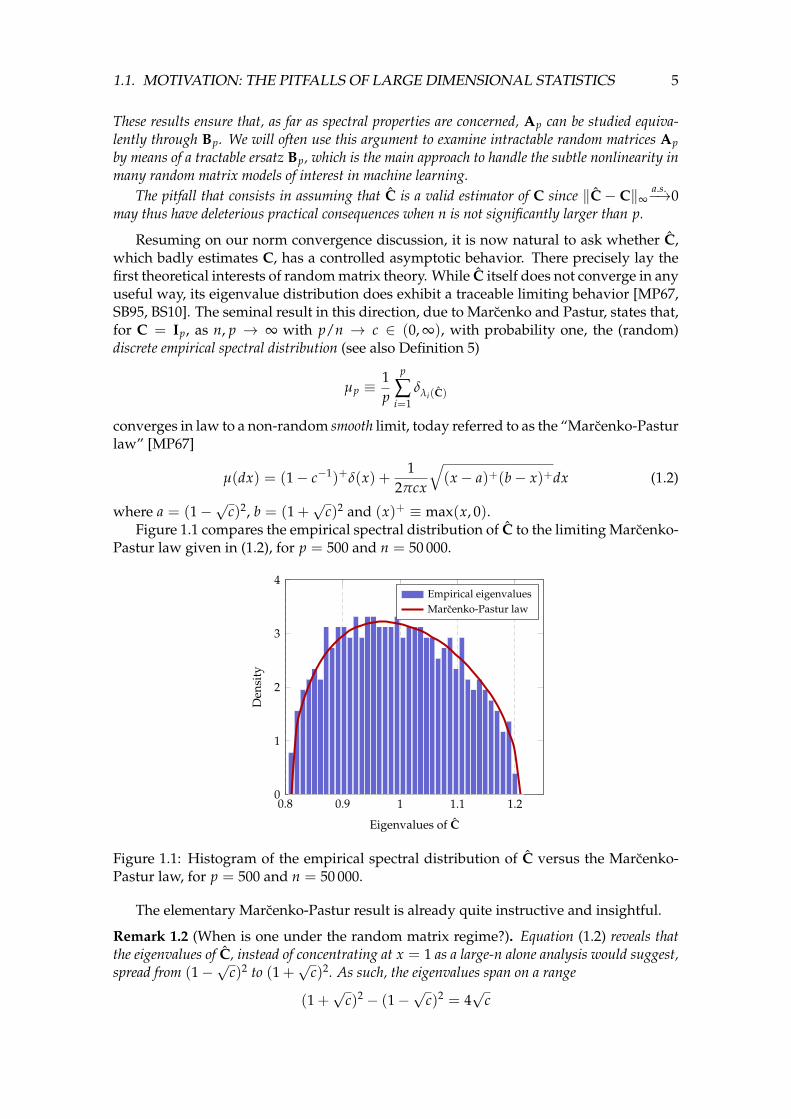
c)2 and (x)+ ≡ max(x, 0).Figure 1.1 compares the empirical spectral distribution of C to the limiting Marcenko-
Pastur law given in (1.2), for p = 500 and n = 50 000.
0.8 0.9 1 1.1 1.20
1
2
3
4
Eigenvalues of C
Den
sity
Empirical eigenvaluesMarcenko-Pastur law
Figure 1.1: Histogram of the empirical spectral distribution of C versus the Marcenko-Pastur law, for p = 500 and n = 50 000.
The elementary Marcenko-Pastur result is already quite instructive and insightful.
Remark 1.2 (When is one under the random matrix regime?). Equation (1.2) reveals thatthe eigenvalues of C, instead of concentrating at x = 1 as a large-n alone analysis would suggest,spread from (1−
√c)2 to (1 +
√c)2. As such, the eigenvalues span on a range
(1 +√
c)2 − (1−√
c)2 = 4√
c

6 CHAPTER 1. INTRODUCTION
which is indeed a slow decaying behavior with respect to c = lim p/n. In particular, for n =100p, where one would expect a sufficiently large number of samples for C to properly estimateC = Ip, one has 4
√c = 0.4 which is a large spread around the mean (and true) eigenvalue 1.
This is visually confirmed by Figure 1.1 for p = 500 and n = 50 000, where the histogram of theeigenvalues is nowhere near concentrated at x = 1. As such, random matrix results will be largelymore accurate than classical asymptotic statistics even when n ∼ 100p. As a telling example,estimating the covariance matrix of each digit from the popular MNIST dataset [LBBH98] usingthe sample covariance, made of no more than 60 000 training samples (and thus about n = 6 000samples per digit) of size p = 28× 28 = 784, is likely a hazardous undertaking.
Remark 1.3 (On universality). Although introduced here in the context of Gaussian distribu-tions for xi, the Marcenko-Pastur law applies to much more general cases. Indeed, the resultremains valid so long that the xi’s have i.i.d. normalized entries of zero mean and unit variance(and even beyond this setting [A+11, EK09, LC19c]). Similar to the law of large numbers instandard statistics, this universality phenomenon commonly arises in random matrix theory andhigh dimensional statistics and helps to justify the wide applicability of the presented theoreticalresults, even to real datasets.
We have seen in this subsection that the sample covariance matrix C, despite being aconsistent estimator of the population covariance C ∈ Rp×p for fixed p as n→ ∞, fails toprovide a precise prediction on the eigenspectrum of C even with n ∼ 100p. The fact thatwe are dealing with large dimensional data vectors has an impact not only on the (direct)estimation of the data covariance or correlation but also on various statistics commonlyused in machine learning methods. In the following subsection, we will discuss howpopular kernel methods behave differently (from our low dimensional intuition) in largedimensional problems, due to the “curse of dimensionality” phenomenon.
1.1.2 Kernel matrices of large dimensional data
Another less known but equally important example of the curse of dimensionality in ma-chine learning involves the loss of relevance of the notion of Euclidean distance betweenlarge dimensional data vectors. To be more precise, we will see in this subsection that,under an asymptotically non-trivial classification setting (that is, ensuring that asymp-totic classification is neither too simple nor impossible), large and numerous data vectorsx1, . . . , xn ∈ Rp extracted from a few-class mixture model tend to be asymptotically atequal distance from one another, irrespective of their mixture class. Roughly speaking, inthis non-trivial setting and under reasonable statistical assumptions on the xi’s, we have
max1≤i 6=j≤n
1p‖xi − xj‖2 − τ
→ 0 (1.3)
for some constant τ > 0 as n, p → ∞, independently of the classes (same or different) of xiand xj (here the distance normalization by p is used for compliance with the notations inthe remainder of the manuscript but has no particular importance).
This asymptotic behavior is extremely counterintuitive and conveys the idea that clas-sification by standard methods ought not to be doable in this large n, p regime. Indeed,in the conventional low dimensional intuition that forged many of the leading machinelearning algorithms of everyday use (such as spectral clustering [NJW02, VL07]), twodata points belong to the same class if they are “close” in Euclidean distance. Here weclaim that, when p is large, data pairs are neither close nor far from each other, regard-less of their belonging to the same class or not. Despite this troubling loss of individual

1.1. MOTIVATION: THE PITFALLS OF LARGE DIMENSIONAL STATISTICS 7
discriminative power between data pairs, we subsequently show that thanks to a collec-tive behavior of all data belonging to the same (few and thus of large size each) classes,asymptotic data classification or clustering is still achievable. Better, we shall see that,while many conventional methods devised from small dimensional intuitions do fail inthe large dimensional regime, some popular approaches (such as the Ng-Jordan-Weissspectral clustering method [NJW02] or the PageRank semi-supervised learning approach[AMGS12]) still function. But the core reasons for their functioning are strikingly differ-ent from the reasons for their initial designs, and they often operate far from optimally.
The non-trivial classification regime2
To get a clear picture of the source of Equation (1.3), we first need to clarify what we referto as the “asymptotically non-trivial” classification setting. Consider the simplest settingof a binary Gaussian mixture classification. We give ourselves a training set x1, . . . , xn ∈Rp of n samples independently drawn from the two-class (C1 and C2) Gaussian mixture
C1 : x ∼ N (µ1, C1)
C2 : x ∼ N (µ2, C2)
each with probability 1/2, for some deterministic µ1, µ2 ∈ Rp, positive definite C1, C2 ∈Rp×p, and assume
Assumption 1 (Covariance scaling). As p→ ∞, we have for a ∈ 1, 2 that
max‖Ca‖, ‖C−1a ‖ = O(1).
In the ideal case where µ1, µ2 and C1, C2 are perfectly known, one can devise a (deci-sion optimal) Neyman-Pearson test. For an unknown x, genuinely belonging to C1, theNeyman-Pearson test to decide on the class of x reads
(x− µ2)TC−1
2 (x− µ2)− (x− µ1)TC−1
1 (x− µ1)C1≷C2
logdet(C1)
det(C2). (1.4)
Writing x = µ1 + C121 z for z ∼ N (0, Ip), the above test is equivalent to
T(x) ≡ 1p
zT(C121 C−1
2 C121 − Ip)z +
2p
∆µTC−12 C
121 z +
1p
∆µTC−12 ∆µ− 1
plog
det(C1)
det(C2)
C1≷C2
0.
(1.5)where we denote ∆µ ≡ µ1 − µ2 that is then normalized by 1/p. Since z ∼ N (0, Ip), UTz
follows the same distribution as z for U ∈ Rp×p an eigenvector basis of C121 C−1
2 C121 − Ip.
As such, the random variable T(x) can be written as the sum of p independent randomvariables. By Lyapunov’s central limit theorem (e.g., [Bil12, Theorem 27.3]), we have, asp→ ∞,
V−12
T (T(x)− T) d−→N (0, 1)
where
T ≡ 1p
tr(C1C−12 )− 1 +
1p
∆µTC−12 ∆µ− 1
plog
det(C1)
det(C2),
VT ≡2p2 ‖C
121 C−1
2 C121 − Ip‖2
F +4p2 ∆µTC−1
2 C1C−12 ∆µ.
2This subsection is extracted from our contribution [CLM18].
8 CHAPTER 1. INTRODUCTION
As a consequence, the classification performance of x ∈ C1 is asymptotically non-trivial(i.e., the classification error neither goes to 0 nor 1 as p→ ∞) if and only if T is of the sameorder of
√VT with respect to p. Let us focus on the difference in means ∆µ by considering
the worst case scenario where the two classes share the same covariance C1 = C2 = C.In this setting, one has from Assumption 1 that
T =1p
∆µTC−1∆µ = O(‖∆µ‖2 p−1),√
VT =2p
√∆µTC−1C−1
2 ∆µ = O(‖∆µ‖p−1)
so that one must have ‖∆µ‖ ≥ O(1) with respect to p (indeed, if ‖∆µ‖ = o(1), theclassification of x with C1 = C2 = C is asymptotically impossible).
Under the critical constraint ‖∆µ‖ = O(1) we move on to considering the case ofdifferent covariances C1 6= C2 in such a way that their difference ∆C ≡ C1 − C2 satisfies‖∆C‖ = o(1). In this situation, by a Taylor expansion of both C−1
2 and det(C2) aroundC1 = C we obtain
T =1p
∆µTC−1∆µ+1
2p‖C−1∆C‖2
F + o(p−1), VT =4p2 ∆µTC−1∆µ+
2p2 ‖C
−1∆C‖2F + o(p−2),
which demands ‖∆C‖ to be at least of order O(p−12 ), so that ‖C−1∆C‖2
F is of orderO(1) (as ‖µ‖) and can have discriminative power, since ‖C−1∆C‖2
F ≤ p‖C−1∆C‖2 ≤p‖∆C‖2, with equality if and only if both C and ∆C are proportional to identity, i.e.,C = ε1Ip and ∆C = ε2Ip. Also, by the Cauchy–Schwarz inequality, we have | tr ∆C| ≤√
tr(∆C2) · tr Ip = O(√
p), with equality (again) if and only if ∆C = εIp, and we musttherefore have | tr ∆C| ≥ O(
√p). This allows us to conclude on the following non-trivial
classification conditions
‖∆µ‖ ≥ O(1), ‖∆C‖ ≥ O(p−1/2), | tr ∆C| ≥ O(√
p), ‖∆C‖2F ≥ O(1). (1.6)
These are the minimal conditions for classification in the case of perfectly known meansand covariances in the following sense: i) if none of the inequalities hold (i.e., if meansand covariances from both classes are too close), asymptotic classification must fail; andii) if at least one of the inequalities is not tight (say if ‖∆µ‖ ≥ O(
√p)), asymptotic classi-
fication becomes (asymptotically) trivially easy.
We shall subsequently see that (1.6) precisely induces the asymptotic loss of distancediscrimination raised in (1.3) but that in the meantime standard spectral clustering meth-ods based on n ∼ p data remain valid in practice.
Asymptotic loss of pairwise distance discrimination
Under the equality case for the conditions in (1.6), the (normalized) Euclidean distancebetween two distinct data vectors xi ∈ Ca, xj ∈ Cb, i 6= j, is given by
1p‖xi − xj‖2 =
1p‖C
12a zi − C
12b zj‖2 − 2
p(µa − µb)
T(C12a zi − C
12b zj) +
1p‖µa − µb‖
2
=1p(zTi Cazi + zTj Cbzj)−
2p
zTi C12a C
12b zj︸ ︷︷ ︸
O(p−1/2)
− 2p(µa − µb)
T(C12a zi − C
12b zj)︸ ︷︷ ︸
O(p−1)
+1p‖µa − µb‖
2︸ ︷︷ ︸O(p−1)
1.1. MOTIVATION: THE PITFALLS OF LARGE DIMENSIONAL STATISTICS 9
where we see again from Lyapunov’s CLT that the second and third terms are of orderO(p−1/2) and O(p−1) respectively, while the last term is of order O(p−1), following di-rectly from the critical condition of (1.6). Denote the average covariance of the two classesC ≡ 1
2 (C1 + C2) so that ‖C‖ = O(1). Note that
1p
E[zTi Cazi] =1p
E[tr(CazizTi )] =1p
tr Ca =1p
tr C +1p
tr(Ca − C) ≡ 12
τ +1p
tr Ca(1.7)
where we introduce τ ≡ 2p tr C = O(1) and Ca ≡ Ca − C for a ∈ 1, 2, the operator
norm of which is of order O(p−1/2) under the critical condition of (1.6).As such, it is convenient to further write
1p
zTi Cazi =1p
tr Ca +
(1p
zTi Cazi −1p
tr Ca
)≡ τ
2+
1p
tr Ca︸ ︷︷ ︸O(p−1/2)
+ ψi︸︷︷︸O(p−1/2)
with ψi ≡ 1p zTi Cazi − 1
p tr Ca = O(p−1/2) again by the CLT and 1p tr Ca = O(p−1/2) under
(1.6). A similar result holds for 1p zTj Cbzj and
1p‖xi − xj‖2 = τ +
1p
tr(Ca + Cb) + ψi + ψj −2p
zTi C12a C
12b zj︸ ︷︷ ︸
O(p−1/2)
− 2p(µa − µb)
T(C12a zi − C
12b zj) +
1p‖µa − µb‖
2︸ ︷︷ ︸O(p−1)
.
This holds regardless of the values taken by a, b. Indeed, one can show with some furtherrefinements that
max1≤i 6=j≤n
1p‖xi − xj‖2 − τ
→ 0
almost surely as n, p→ ∞, as previously claimed in (1.3).
To visually confirm the joint convergence of the data distances, Figure 1.2 displaysthe content of the Gaussian heat kernel matrix K with Kij = exp
(− 1
2p‖xi − xj‖2)
(whichis, therefore, a Euclidean distance-based similarity measure between data points) and theassociated second top eigenvector v2 for a two-class Gaussian mixture x ∼ N (±µ, Ip)with µ = [2; 0p−1]. For a constant n = 500, we take p = 5 in Figure 1.2a and p = 250 inFigure 1.2b.
While the “block-structure” in Figure 1.2a agrees with the low dimensional intuitionthat data vectors from the same class are “closer” to one another, corresponding to di-agonal blocks with larger values (since exp(−x/2) decreases with the distance) than innon-diagonal blocks, this intuition collapses when large dimensional data vectors areconsidered. Indeed, in the large data setting of Figure 1.2b, all entries (but obviously onthe diagonal) of K have approximately the same value, which we now know from (1.3)is exp(−1).
This is no longer surprising to us. However, what remains surprising at this stageof our analysis is that the eigenvector v2 of K is not affected by the asymptotic loss ofclass-wise discrimination of individual distances. Thus spectral clustering seems to workequally well for p = 5 or p = 250, despite the radical and intuitively destructive change

10 CHAPTER 1. INTRODUCTION
K =
v2 =
(a) p = 5, n = 500.
K =
v2 =
(b) p = 250, n = 500.
Figure 1.2: Kernel matrices K and the second top eigenvectors v2 for small and largedimensional data X = [x1, . . . , xn] ∈ Rp×n with x1, . . . , xn/2 ∈ C1 and xn/2+1, . . . , xn ∈ C2.
in the behavior of K for p = 250. An answer to this question will be given in Section 3.1.1.We will also see that not all kernel choices can reach the same (non-trivial) classificationrates, in particular, the popular Gaussian kernel will be shown to be sub-optimal in thisrespect.
1.1.3 Summary of Section 1.1
In this section, we discussed two simple, yet counterintuitive, examples of common pit-falls in handling large dimensional data.
In the sample covariance matrix example in Section 1.1.1, we made the importantremark of the loss of equivalence between matrix norms in the random matrix regime wherethe data/feature dimension p and their number n are both large and comparable, whichis at the source of many intuition errors. We in particular insist that, for matrices An, Bn ∈Rn×n of large sizes
∀i, j, (An − Bn)ij → 0 6⇒ ‖An − Bn‖ → 0 (1.8)
in operator norm.We also realized, from a basic reading of the Marcenko-Pastur theorem, that the ran-
dom matrix regime arises more often than one may think: while n/p ∼ 100 may seemlarge enough a ratio for classical asymptotic statistics to be accurate, random matrix the-ory is, in general, a far more appropriate tool (with as much as 20% gain in precision forthe estimation of the covariance eigenvalues).
In Section 1.1.2, we gave a concrete machine learning classification example of themessage in (1.8) above. We saw that, in the practically most relevant scenario of non-trivial (not too easy, not too hard) large data classification tasks, the distance betweenany two data vectors “concentrates” around a constant (1.3), regardless of their respec-tive classes. Yet, since again (Kn)ij → τ does not imply that ‖Kn − τ1n1Tn ‖ → 0 in

1.2. RANDOM KERNELS, RANDOM NEURAL NETWORKS AND BEYOND 11
operator norm, we understood that, thanks to a collective effect of the small but similarly“oriented” (informative) fluctuations, kernel spectral clustering remains valid for largedimensional problems.
In a nutshell, the fundamental counterintuitive yet mathematically addressable changesin behavior of large dimensional data have two major consequences to statistics and ma-chine learning: i) most algorithms, originally developed under a low dimensional intu-ition, are likely to fail or at least to perform inefficiently, yet ii) by benefiting from theextra degrees of freedom offered by large dimensional data, random matrix theory is aptto analyze, improve, and evoke a whole new paradigm for large dimensional learning.
In the following sections of this chapter, we introduce the basic settings under whichwe work, the machine learning models that we are interested in, as well as the majorchallenges that we face. In Section 1.2 we discuss three closely related topics: randomkernel matrices, random (nonlinear) feature maps, and simple random neural networks.Under a natural and rather general mixture model, we characterize the eigenspectrum ofa large kernel matrix and predict the performance of the kernel ridge regressor (whichis an explicit function of the kernel function). Random feature maps that are designedto approximate large kernel matrices, take exactly the same form as a single-hidden-layer NN model with random weights. As a consequence, studying such a network isequivalent to assess the performance of a random feature-based kernel ridge regression,and is thus closely connected to the kernel ridge regression model.
1.2 Random Kernels, Random Neural Networks and Beyond
Randomness is intrinsic to machine learning, as the probabilistic approach is one of themost common tools used to study the performances of machine learning methods. Manymachine learning algorithms are designed to estimate some unknown probability dis-tribution, to separate the mixture of several different distribution classes, or to generatenew samples following some underlying distribution.
Randomness has various sources in machine learning: it may come from the basic sta-tistical assumption that the data are (independently or not) drawn from some probabilitydistribution, from a possibly random search of the hyperparameters of the model (thepopular dropout technique in training DNNs [SHK+14]) or from the stochastic nature ofthe optimization methods applied (e.g., stochastic gradient descent method and its vari-ants). There are also numerous machine learning methods that are intrinsically random,where randomness is not used to enhance a particular part of the model but is indeed thebasis of the model itself, for example in the case of random weights neural networks (aswe shall discuss later in Section 1.2.2) as well as many tree-based models such as randomforests [Bre01] and extremely randomized trees [GEW06].
Let us first focus on the randomness from data by introducing the following multi-variate mixture modeling for the input data, which will be considered throughout thismanuscript.
Definition 1 (Multivariate mixture model). Let x1, . . . , xn ∈ Rp be n random vectors drawnindependently from a K-class mixture model C1, . . . , CK so that each class Ca has cardinality nafor a = 1, . . . , K and ∑K
a=1 na = n. We say xi ∈ Ca if
xi = µa + C12a zi

12 CHAPTER 1. INTRODUCTION
for some deterministic µa ∈ Rp, symmetric and positive definite Ca ∈ Rp×p and some randomvector zi with i.i.d. zero mean and unit variance entries. In particular, we say xi follows a K-classGaussian mixture model (GMM) if zi ∼ N (0, Ip).
The assumption that the data xi are a linear or affine transformation of i.i.d. randomvectors zi characterizes the first and second order statistics of the underlying data distri-bution. Many RMT results such as the popular Marcenko-Pastur law in (1.2), as stated inRemark 1.3, hold universally with respect to the distribution of the independent entries.As such, it often suffices to study the (most simple) Gaussian case to reach a universalconclusion. We will come back to this point with some fundamental RMT results in Sec-tion 2.2 and discuss some possible limitations of this “universality” in RMT in Chapter 5.
We insist here that this multivariate mixture model setting for the input data/featuremakes the crucial difference between our works and other existing RMT-based analysesof machine learning systems, such as those of L. Zdeborova and F. Krzakala [KMM+13,SKZ14], or those of J. Pennington [PW17, PW17, PSG17]. In all these contributions, theauthors are routinely interested in very homogeneous problems with simple data struc-tures, e.g., xi ∼ N (0, Ip), which makes their analyses more tractable and leads to verysimple and more straightforward intuitions or conclusions. On the opposite, we take themore natural choice of mixture model with more involved structures, as in the case ofGMM in Definition 1. This enhances the practical applicability of our results, as shallbe demonstrated throughout this manuscript: when compared to experiments on com-monly used datasets, our theoretical results constantly exhibit an extremely close matchto practice. This observation, together with the underlying “universality” argument fromRMT, conveys a strong applicative motivation for our works.
As we shall always work in the regime where both n, p are large and comparable, wewill, according to the discussions in Section 1.1.2, position ourselves under the followingnon-trivial regime where the separation of the K-class mixture above is neither too easynor impossible as n, p→ ∞.
Assumption 2 (Non-trivial classification). As n→ ∞, for a ∈ 1, . . . , K
1. p/n = c→ c ∈ (0, ∞) and na/n = ca → ca ∈ (0, 1).
2. ‖µa‖ = O(1) and max‖Ca‖, ‖C−1a ‖ = O(1) with | tr Ca | = O(
√p), ‖Ca‖2
F =
O(√
p) for Ca ≡ Ca −∑Ki=1
nin Ci.
Assumption 2 is a natural extension of the non-trivial classification condition in (1.6)to the general K-class setting.
Under a GMM for the input data that satisfies Assumption 2, we aim to investigatethe (asymptotic) performance of any machine learning method of interest, in the largedimensional regime where n, p → ∞ and p/n → c ∈ (0, ∞). However, in spite of a hugenumber of well-established RMT results, the “exact” performance (as a function of thedata statistics µ, C and the problem dimensionality n, p) still remains technically out ofreach, for most machine learning algorithms.
The major technical difficulty that prevents existing RMT results from being applieddirectly to understand these machine learning systems is the nonlinear and sometimesimplicit nature of these models. Powerful machine learning methods are commonly builton top of highly complex and nonlinear features, which make the evaluation of thesemethods less immediate than linear and explicit methods. As a consequence, we needa proper adaptation of the matrix-based classical RMT results to handle the entry-wise

1.2. RANDOM KERNELS, RANDOM NEURAL NETWORKS AND BEYOND 13
nonlinearity (e.g., the kernel function or the activation function in neural networks) or theimplicit solutions arising from optimization problems (of logistic regression for instance).
In this section, in pursuit of a satisfying answer to these aforementioned technicaldifficulties, we review some recent advances in RMT in this vein, starting from largekernel matrices.
1.2.1 Random matrix consideration of large kernel matrices
Large kernel matrices and their spectral properties
In a broad sense, kernel methods are at the core of many, if not most, machine learningalgorithms. For a given data set x1, . . . , xn ∈ Rp, most learning mechanisms aim to extractthe structural information of the data (to perform classification for instance) by assessingthe pairwise comparison k(xi, xj) for some affinity metric k(·, ·) to obtain the matrix
K ≡
k(xi, xj)n
i,j=1 . (1.9)
The “cumulative” effect of these comparisons for numerous (n 1) data is at the heartof a broad range of applications: from supervised learning methods of maximum mar-gin classifier such as support vector machines (SVMs), kernel ridge regression or kernelFisher discriminant, to kernel spectral clustering and kernel PCA that work in a totallyunsupervised manner.
The choice of the affinity function k(·, ·) is central to a good performance of the learn-ing method. A typical viewpoint is to assume that data xi and xj are not directly compa-rable (e.g., not linearly separable) in their ambient space but that there exists a convenientfeature mapping φ : Rp → H that “projects” the data to some (much higher or even infinitedimensional) feature space H where φ(xi) and φ(xj) are more amenable to comparison,for example, can be linearly separable by a hyperplane inH.
While the dimension of the feature space H can be much higher than that of the data(p), with the so-called “kernel trick” [SS02] one can avoid the evaluation of φ(·) andinstead work only with the associated kernel function k : Rp ×Rp 7→ R that is uniquelydetermined by
k(xi, xj) = φ(xi)Tφ(xj) (1.10)
via Mercer’s theorem [SS02]. Some commonly used kernel functions are the radial ba-
sis function (RBF, or Gaussian, or heat) kernel k(xi, xj) = exp(− ‖xi−xj‖2
2σ2
), the sigmoid
kernel tanh(xTi xj + c) and polynomial kernels (xTi xj + c)d. These kernel-based learningalgorithms have been extensively studied both theoretically and empirically for their fea-ture extraction power in highly nonlinear data manifolds, before the recent “rebirth” ofneural networks.
But only very recently has the large dimensional (p ∼ n 1) nature of the datastarted to be taken into consideration for kernel methods. We have seen in Section 1.1.2empirical evidence showing that the kernel matrix K behaves dramatically differentlyfrom its low dimensional counterpart. In the following, we review some theoretical ex-planations of this counterintuitive behavior provided by RMT analyses.
To assess the eigenspectrum behavior of K for n, p both large and comparable, theauthor of [EK10b] considered kernel matrices K with “shift-invariant” type kernel func-tions k(xi, xj) = f (‖xi − xj‖2/p) or “inner-product” kernel f (xTi xj/p) for some nonlinearand locally smooth function f . It was shown that the kernel matrix K is asymptotically

14 CHAPTER 1. INTRODUCTION
equivalent to a more tractable random matrix K in the sense of operator norm, as statedin the following theorem.
Theorem 1.1 (Theorem 2.1 in [EK10b]). For inner-product kernel f (xTi xj/p) and xi = C12 zi
with positive definite C ∈ Rp×p satisfying Assumption 1 and random vector zi ∈ Rp withi.i.d. zero mean, unit variance and finite 4+ ε (absolute) moment entries and f three-times differ-entiable in a neighborhood of 0, we have
‖K− K‖ → 0
in probability as n, p→ ∞ with p/n→ c ∈ (0, ∞), where
K =
(f (0) +
f ′′(0)2p2 tr(C2)
)1n1Tn +
f ′(0)p
XTX +(
f(τ
2
)− f (0)− τ
2f ′(0)
)In (1.11)
with τ ≡ 2p tr C > 0.
We provide here only the intuition for this result in the inner-product kernel f (xTi xj/p)case with Gaussian zi ∼ N (0, Ip). The shift-invariant case can be treated similarly. Toprove the universality with respect to the distribution of entries of zi, a more cumbersomecombinatoric approach was adopted in [EK10b], which is likely unavoidable.
Intuition of Theorem 1.1. The proof is based on an entry-wise Taylor expansion of the ker-nel matrix K, which naturally demands the kernel function f to be locally smooth aroundzero. More precisely, we obtain, using Taylor expansion of f (x) around x = 0 that, fori 6= j,
Kij = f (xTi xj/p) = f (0) +f ′(0)
pxTi xj +
f ′′(0)p2 (xTi xj)
2 + Tij
with some higher order (≥ 3) terms Tij that contain higher order derivatives of f . Notethat Tij typically contains terms of the form (xTi xj/p)κ for κ ≥ 3 so that Tij is of orderO(p−3/2), uniformly on i 6= j, as a result of xTi xj/p = O(p−1/2) by the CLT. As such, thematrix Tij δi 6=j1≤i,j≤n (of size n× n and with zeros on its diagonal) can be shown to havea vanishing operator norm as n, p→ ∞ since
‖Tij δi 6=j1≤i,j≤n‖ ≤ n‖Tijδi 6=j1≤i,j≤n‖∞ = o(1)
as n, p → ∞ with p/n → c ∈ (0, ∞). We then move on to the second order termf ′′(0)
p2 (xTi xj)2, the expectation of which is given by
f ′′(0)p2 E(xTi xj)
2 =f ′′(0)
p2 Exi tr(
xTi Exj [xjxTj ]xi
)=
f ′′(0)p2 tr(C2) = O(p−1)
where we use the linearity of the trace operator to push the expectation inside, togetherwith the fact that ‖C‖ = O(1). In matrix form this gives,
f ′′(0)p2 E[(xTi xj)
2δi 6=j]1≤i,j≤n =f ′′(0)
p2 tr(C2)(1n1Tn − In)
which is of operator norm of order O(1), even without the diagonal term f ′′(0)p2 tr(C2)In
(the operator norm of which is of order O(p−1) and thus vanishing, also note that weleave the diagonal untreated for the moment). With concentration arguments we canshow the fluctuation (around the expectation) of this second order term also has a vanish-ing operator norm as n, p → ∞ with p/n → c > 0, which, together with easy treatmentof the diagonal terms, concludes the proof.

1.2. RANDOM KERNELS, RANDOM NEURAL NETWORKS AND BEYOND 15
This operator norm consistent approximation ‖K − K‖ → 0, as discussed in Re-mark 1.1, provides a direct access to the limiting spectral measure (if it exists), the isolatedeigenvalues and associated eigenvectors that are of central interest in spectral clusteringor PCA applications, as well as the regression or label/score vectors, of (functions of) theintractable kernel matrix K, via the study of the more tractable random matrix model K,according to Weyl’s inequality (see Lemma 2.10).
The asymptotic equivalent kernel matrix K is the sum of three matrices: i) a rank onematrix proportional to 1n1Tn , ii) the identity matrix that makes a constant shift of all eigen-values and iii) a rescaled version of the standard Gram matrix 1
p XTX. The eigenvaluedistribution of the Gram matrix, or equivalently of the sample covariance matrix model1p XXT (via Sylvester’s identity in Lemma 2.3) has been intensively studied in the randommatrix literature [SB95], and we shall talk about this model at length in Section 2.2.3. Thelow rank (rank one here) perturbation of a random matrix model, is known under thename of “spiked model” and has received considerable research attention in the RMTcommunity [BAP05]; we will come back to this point in more details in Section 2.3.
On closer inspection of (1.11), we see that K is in essence a local linearization of thenonlinear K, in the sense that the nonlinear function f (x) is evaluated solely in the neigh-borhood of x = 0. This is because by the CLT we have xTi xj/p = O(p−
12 ) for i 6= j, and
entry-wise speaking, all off-diagonal entries are constantly equal to f (0) to the first or-der. As such, the nonlinear function f acts only in a “local” manner around 0: all smoothnonlinear f with the same values of f (0), f ′(0) and f ′′(0) have the same expression of K,up to a constant shift of all eigenvalue due to f (τ/2)In, and consequently have the same(asymptotic) performance on all kernel-based spectral algorithms.
In [EK10a] the author considered an “information-plus-noise” model for the data,where each observation consists of two parts: one from a “low dimensional” structureyi ∈ Rp (e.g., with its `0 norm ‖yi‖0 = O(1)) that is considered the “signal” as wellas the informative part of the data and the other being high dimensional noise. Thismodeling indeed assumes that data are randomly drawn from, not exactly a fixed andlow dimensional manifold, but somewhere “nearby” such that the resulting observationsare perturbed with additive high dimensional noise, more precisely
xi = yi + C12 zi
where yi denotes the random “signal” part of the observation and zi the high dimensionnoise part that is independent of yi. The proof techniques are basically the same as in[EK10b]. However, by assuming that all xi’s drawn from the same distribution, this resultis not sufficient for the understanding of K in a more practical classification context.
More recently in [CBG16], the authors considered the shift-invariant kernel f (‖xi −xj‖2/p), under a more involved K-class Gaussian mixture model (GMM, see Definition 1)for the data, that is of more practical interest from a machine learning standpoint, andinvestigated more precisely the eigenspectrum behavior for a kernel spectral clusteringpurpose. Not only the kernel matrix K but also the associated (normalized) Laplacianmatrix L defined as
L ≡ nD−12 KD−
12
are considered in [CBG16], where D ≡ diag(K1n) denotes the so-called “degree matrix”of K. While the authors followed the same technical approach as in [EK10b], the factthat they considered a Gaussian mixture modeling provides rich insights into the impactof nonlinearity in kernel spectral clustering applications. For the first time, the exact

16 CHAPTER 1. INTRODUCTION
stochastic characterization of the isolated eigenpairs are given, as a function of the datastatistics (µ, C), problem dimensionality n, p, as well as the nonlinear f in a local manner.
Built upon the investigation of K in [CBG16], we evaluate the exact performance ofthe kernel ridge regression (or least squares support vector machine, LS-SVM) in classi-fying a two-class GMM, in the following contributions.
(C1) Zhenyu Liao and Romain Couillet. Random matrices meet machine learning: alarge dimensional analysis of LS-SVM. In 2017 IEEE International Conference onAcoustics, Speech and Signal Processing (ICASSP), pages 2397–2401, 2017.
(J1) Zhenyu Liao and Romain Couillet. A large dimensional analysis of least squaressupport vector machines. IEEE Transactions on Signal Processing, 67(4):1065–1074,2019.
In a nutshell, we consider the following (soft) output decision function from the LS-SVM formulation
h(x) = βTk(x) + b, β = Q(y− b1n), b =1Tn Qy1Tn Q1n
(1.12)
for k(x) ≡ f (‖x− xi‖2/p)ni=1 ∈ Rn and Q =
(K + n
λ In)−1 the so-called resolvent of the
kernel matrix K (see Definition 4). By showing that h(x) can be (asymptotically) well ap-proximated by a normally distributed random variable, we obtain the exact asymptoticclassification performance of LS-SVM. The minimum orders of magnitude distinguish-able by an LS-SVM classifier are given by
‖∆µ‖ = O(1), | tr ∆C| = O(√
p), ‖∆C‖2F = O(p)
for ∆µ = µ1 − µ2 and ∆C = C1 − C2. This is very close to the theoretical optimum in theoracle setting in (1.6) and is the best rate reported in [CLM18].
Perhaps more importantly, when tested on several real-world datasets such as theMNIST [LBBH98] and Fashion MNIST [XRV17] image datasets, a surprisingly close matchis observed between theory and practice, thereby conveying a strong applicative motiva-tion for the study of simple GMM in a high dimensional setting. We will continue thisdiscussion in more details and justify that this observation is in fact not that surprising inSection 3.1.1.
All works above are essentially based on a local expansion of the kernel function f ,which follows from the “concentration” of the similarity measure ‖xi − xj‖2/p or xTi xj/paround a single value of the smooth domain of f . More precisely, due to the independencebetween two data vectors xi, xj, the diagonal and off-diagonal entries of K behave in atotally different manner. Consider Kij = f (xTi xj/p) with xi ∼ N (0, Ip); we have roughlyf (1) on and f (0) off the diagonal of K, so that most entries (of order O(n2)) of K evaluatethe nonlinear function f around zero. This leads to the “local linearization” of f in theexpression of K in Theorem 1.1 and thereby disregards most of the domain of f .
On the other hand, since xTi xj/√
p→ N (0, 1) in distribution as p→ ∞ (and is thus oforder O(1) with high probability), it appears that f (xTi xj/
√p) is a more natural scaling to
avoid an asymptotic linearization of the nonlinear K. Nonetheless, in this case, all diag-onal entries become ‖xi‖2/
√p = O(
√p) and thus evaluate f asymptotically at infinity,
which is again another “improper scaling”, but only on the diagonal of K.

1.2. RANDOM KERNELS, RANDOM NEURAL NETWORKS AND BEYOND 17
In the dot product model f (xTi xj/√
p), the entries will not “concentrate” at f (0). Al-ternative tool is thus needed in the place of the Taylor expansion, so as to handle the non-linear function f in this case. This more naturally scaling model was studied in [CS13],where the authors considered the dot product kernel matrix K, the (i, j) entry of which isgiven by
Kij =
f (xTi xj/
√p)/√
p for i 6= j0 for i = j
. (1.13)
The more natural√
p normalization inside f helps, as discussed above, avoid the non-linear K (asymptotically) acting as a linear model XTX, while the
√p scaling outside is
simply convenient to ensure the operator norm ‖K‖ is order O(1) for n, p large. Notethat the diagonal elements are discarded since they are now “improperly scaled” for theevaluation by f .
Again, we are interested in the spectral property of the kernel matrix K defined in(1.13). For xi ∼ N (0, Ip), the empirical spectral measure µn = 1
n ∑ni=1 δλi(K) (see Definition 5)
of K has an asymptotically deterministic behavior as n, p → ∞ with p/n → c ∈ (0, ∞).This limiting spectral measure of K was first characterized in [CS13] and then generalizedin [DV13] to handle random vectors xi with i.i.d. entries of zero mean, unit variance andfinite higher order moments, as summarized in the following theorem.
Theorem 1.2 (Theorem 3.4 in [CS13], Theorem 3 in [DV13]). Under some regularity con-dition for the kernel function f (see Assumption 3 below), the empirical spectral measure of Kconverges weakly and almost surely, as n, p → ∞ with p/n → c ∈ (0, ∞), to a probabil-ity measure µ. The latter is uniquely defined through its Stieltjes transform m : C+ → C+,z 7→
∫(t− z)−1µ(dt) (see also Definition 6 in Section 2.2), given as the unique solution in C+
of the cubic equation3
− 1m(z)
= z +a2
1m(z)c + a1m(z)
+ν− a2
1c
m(z)
with a1 = E[ξ f (ξ)] and ν = Var[ f (ξ)] ≥ a21 for standard Gaussian ξ ∼ N (0, 1).
The technical approach to achieve Theorem 1.2 is rather different from that of Theo-rem 1.1. Instead of performing a local Taylor expansion of f , the authors of [CS13, DV13]rely on the theory of orthogonal polynomials, in particular, of the class of Hermite poly-nomials defined with respect to the standard Gaussian distribution [AS65, AAR00]. Thisthus allows for a polynomial approximation of the nonlinear function f as long as it issquare-integrable, and thus covers naturally non-differentiable kernel functions. Someuseful concepts from the theory of orthogonal polynomial are recalled as follows.
For a probability measure µ, we denote the set of orthogonal polynomials with respectto the scalar product 〈 f , g〉 =
∫f gdµ as Pl(x), l = 0, 1, . . ., obtained from the Gram-
Schmidt procedure on the monomials 1, x, x2, . . . such that P0(x) = 1, Pl is of degreel and 〈Pl1 , Pl2〉 = δl1−l2 . By the Riesz-Fischer theorem [Rud64, Theorem 11.43], for anyfunction f ∈ L2(µ), the set of squared integrable functions with respect to 〈·, ·〉, one canformally expand f as
f (x) ∼∞
∑l=0
al Pl(x), al =∫
f (x)Pl(x)dµ(x) (1.14)
3C+ ≡ z ∈ C, =[z] > 0. We also recall that, for m(z) the Stieltjes transform of a measure µ, µ canbe obtained from m(z) via µ([a, b]) = limε↓0
1π
∫ ba =[m(x + ıε)]dx for all a < b continuity points of µ. See
Section 2.1.2 for more details.

18 CHAPTER 1. INTRODUCTION
where “ f ∼ ∑∞l=0 Pl” indicates that ‖ f −∑N
l=0 Pl‖ → 0 as N → ∞ (and ‖ f ‖2 = 〈 f , f 〉).To ensure the polynomial approximation is accurate when truncated at a large but
finite degree L, we assume the following assumption holds.
Assumption 3. For each p, let ξp = xTi xj/√
p and let Pl,p(x), l ≥ 0 be the set of orthonormalpolynomials with respect to the probability measure µp of ξp. For f ∈ L2(µp) for each p, i.e.,
f (x) ∼∞
∑l=0
al,pPl,p(x)
for al,p defined in (1.14), we demand that
1. ∑∞l=0 al,pPl,p(x)µp(dx) converges in L2(µp) to f (x) uniformly over large p,
2. as p → ∞, ∑∞l=1 |al,p|2 → ν ∈ [0, ∞). Moreover, for l = 0, 1, 2, al,p converges and we
denote a0, a1 and a2 their limits, respectively.
3. a0 = 0.
Since ξp → N (0, 1) as p → ∞, the limiting parameters a0, a1, a2 and ν are simply(generalized) moments of the standard Gaussian measure involving f . Precisely,
a0 = E[ f (ξ)], a1 = E[ξ f (ξ)], a2 =E[(ξ2 − 1) f (ξ)]√
2=
E[ξ2 f (ξ)]− a0√2
, ν = Var[ f (ξ)]
for ξ ∼ N (0, 1). These parameters are of crucial significance in determining the eigen-spectrum behavior of K. For example, the limiting spectral measure is uniquely de-termined by a1 and ν as per Theorem 1.2. The last assumption a0 = 0 is demandedhere mainly for technical convenience and will not affect the classification performancein practice, as it adds a non-informative rank one perturbation of the form a0(1n1Tn −In)/√
p to the kernel matrix.The proof of Theorem 1.2 calls for some standard algebraic and probabilistic manipu-
lations in RMT, that will be introduced in Chapter 2. For self-consistency, we include theintuitive proof for Theorem 1.2 in Section A.1.1 of the appendix.
Theorem 1.2 only gives the (limiting) eigenvalue distribution of the kernel matrix Kin (1.13) under a null model which, from a machine learning perspective, is not sufficientto decide for example how to choose f with respect to the data/task at hand. Comparedto [CBG16], an important piece of the mixture models is still missing, which leads to ourfollowing investigation.
(C2) Zhenyu Liao and Romain Couillet. Inner-product kernels are asymptoticallyequivalent to binary discrete kernels, 2019.
In this contribution we provide, as in Theorem 1.1, a more accessible random matrixK that is asymptotically equivalent to K, under a two-class multivariate mixture model(as in Definition 1) for data with covariance Ca = Ip + Ea that satisfies the non-trivialclassification condition of Assumption 2.
Interestingly, K is (again) nothing but the sum of two matrices: i) the null model KNcharacterized in Theorem 1.2 that depends on f via the two coefficients a1 and ν and ii)a low rank and informative matrix KI that only depends on a1 and a2. This means that,
1.2. RANDOM KERNELS, RANDOM NEURAL NETWORKS AND BEYOND 19
instead of a local behavior of f as in [EK10b, CBG16], the classification performance ofthe properly scaled dot product kernel f (xTi xj/
√p) is related to f in a more “global”, yet
still simple, way only via the three parameters a1, a2 and ν.On the downside, it must be pointed out that, the studies performed in [CS13, DV13]
(as well as in [LC19a] above) only cover the case of identity covariance C = Ip. By intro-ducing an arbitrary covariance C and considering xi = C
12 zi for zi having i.i.d. entries, the
limiting spectral measure of K becomes technically more challenging since it breaks mostof the orthogonality properties of the orthogonal polynomial approach in the proofs. Butit is a needed extension in pursuit of the general multivariate mixture model, and to com-pare the performance between different scaling strategies, which is of significant interestfor future investigation.
Random feature approximation of kernels
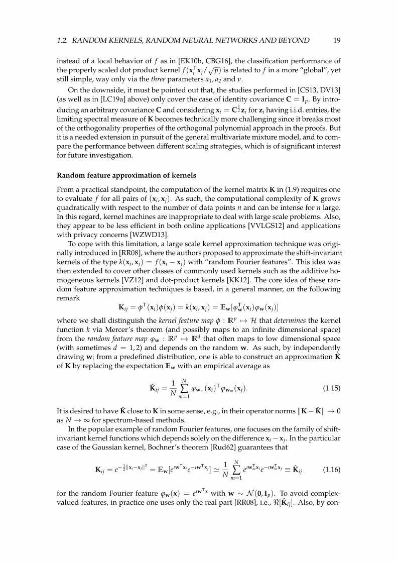
From a practical standpoint, the computation of the kernel matrix K in (1.9) requires oneto evaluate f for all pairs of (xi, xj). As such, the computational complexity of K growsquadratically with respect to the number of data points n and can be intense for n large.In this regard, kernel machines are inappropriate to deal with large scale problems. Also,they appear to be less efficient in both online applications [VVLGS12] and applicationswith privacy concerns [WZWD13].
To cope with this limitation, a large scale kernel approximation technique was origi-nally introduced in [RR08], where the authors proposed to approximate the shift-invariantkernels of the type k(xi, xj) = f (xi − xj) with “random Fourier features”. This idea wasthen extended to cover other classes of commonly used kernels such as the additive ho-mogeneous kernels [VZ12] and dot-product kernels [KK12]. The core idea of these ran-dom feature approximation techniques is based, in a general manner, on the followingremark
Kij = φT(xi)φ(xj) = k(xi, xj) = Ew[ϕTw(xi)ϕw(xj)]
where we shall distinguish the kernel feature map φ : Rp 7→ H that determines the kernelfunction k via Mercer’s theorem (and possibly maps to an infinite dimensional space)from the random feature map ϕw : Rp 7→ Rd that often maps to low dimensional space(with sometimes d = 1, 2) and depends on the random w. As such, by independentlydrawing wi from a predefined distribution, one is able to construct an approximation Kof K by replacing the expectation Ew with an empirical average as
Kij =1N
N
∑m=1
ϕwm(xi)Tϕwm(xj). (1.15)
It is desired to have K close to K in some sense, e.g., in their operator norms ‖K− K‖ → 0as N → ∞ for spectrum-based methods.
In the popular example of random Fourier features, one focuses on the family of shift-invariant kernel functions which depends solely on the difference xi− xj. In the particularcase of the Gaussian kernel, Bochner’s theorem [Rud62] guarantees that
Kij = e−12 ‖xi−xj‖2
= Ew[eıwTxi e−ıwTxj ] ' 1N
N
∑m=1
eıwTmxi e−ıwT
mxj ≡ Kij (1.16)
for the random Fourier feature ϕw(x) = eıwTx with w ∼ N (0, Ip). To avoid complex-valued features, in practice one uses only the real part [RR08], i.e., <[Kij]. Also, by con-
20 CHAPTER 1. INTRODUCTION
sidering various distributions of w, several other shift-invariant kernels can be approxi-mated, including the Laplacian and Cauchy kernels, within the general random Fourierfeature framework.
We close this subsection with the final remark that, by cascading the Gaussian wm’sas row vectors, we obtain a random Gaussian matrix W ∈ RN×p, the entries of which areindependent standard Gaussian random variables, i.e., Wij ∼ N (0, 1). Then, accordingto (1.16) we have
<[Kij] =1N
σ1(Wxi)Tσ1(Wxj) +
1N
σ2(Wxi)Tσ2(Wxj) (1.17)
for σ1(t) = cos(t) and σ2(t) = sin(t), which coincides with the Gram matrix of the single-layer neural network model with random weights W and cosine+sine activation func-tions, as detailed in the following subsection.
1.2.2 Random neural networks
A fundamental link exists between random feature maps (and thus random kernel ma-trices) and neural networks with random weights. Neural networks (NNs) with randomweights have their roots in the pioneering works on the perceptron [Ros58] and havethen been successively revisited and analyzed in a number of works, both in the feed-forward [SKD92, ASD96] and the recurrent case [Gel93]. More recently, some of theserandomized NN models (the so-called extreme learning machine [HZDZ12] as an exam-ple for the feed-forward case and the echo state network [Jae01] for the recurrent one)have been shown to achieve satisfactory performances in some problems (see examplesin the next paragraph), with a relatively short training time and low model complexity.We refer the readers to [SW17] for a complete overview of randomness in NN models.
Random neural networks are more than a “cheap” way to solve less efficiently adifficult problem, given the limited computational resources at hand. On the contrary,they work sufficiently well in many practical scenarios [HZDZ12] and can even some-times achieve remarkable accuracies that are comparable to deep and finely tuned struc-tures, in a large number of applications [LML+14]. This seemingly counterintuitivefact is perhaps the key to a deeper comprehension of the intrinsic properties of differ-ent NN architectures. Taking the example of convolutional neural networks (CNNs),it was observed in [JKL09] that, for small datasets, completely random filters are suffi-cient to propagate useful information through a rectified linear (ReLU) network. Thisobservation was used to argue for the significance of ReLU nonlinearities and the (con-volutional) pooling operation in image classification problems, as also pointed out in[PDDC09, SKC+11, CP11b, GSB16], and in many other tasks such as image reconstruc-tion [HWH16], denoising and super-resolution [UVL18].
Random NNs have the advantage of being mathematically more tractable, at the sametime preserving the “structural” properties of these elaborate learning systems, e.g., theuse of appropriate nonlinear functions in DNNs or convolutional filters in CNNs. Thestudy of random NNs can, therefore, shed novel light on the design of more advancedNN models.
In the training procedure of modern NNs, optimization methods such as (stochastic)gradient descent and its variants are always initialized randomly, with the NN weightsdrawn randomly from a (properly scaled) normal distribution. In this regard, NNs withrandom weights are essentially the initial states of well-trained NNs, and can providehelpful insight into the understanding of modern DNNs, e.g., to accelerate training, at

1.2. RANDOM KERNELS, RANDOM NEURAL NETWORKS AND BEYOND 21
least at the very initial stage, by examining the eigenspectrum behavior of the input-output Jacobian matrix [PSG17], or to gain theoretical insights into the geometric proper-ties of DNNs [DLT+18, AZLS18]. In these works, the network weights, or training data,or both of them, are typically assumed to be normally distributed to facilitate theoreticalassessment.
In this manuscript, we focus only on feed-forward NNs. For random recurrent NNs,RMT-based analyses have also been established, but are mainly restricted to the linearcase [CWSA16].
Let us consider the random weights feed-forward NN with a single hidden layer asin Figure 1.3.
X ∈ Rp×n
σσσσσ
Σ ≡ σ(WX) ∈ RN×nβTΣ
W ∈ RN×pβ ∈ RN×d
Figure 1.3: Illustration of a single-hidden-layer random NN
For a data matrix X =[x1, . . . , xn
]∈ Rp×n, we denote Σ ∈ RN×n the output of
the middle layer comprising of N neurons in total (also referred to as the random featurematrix) of X by premultiplying some random weight matrix W ∈ RN×p with i.i.d. stan-dard Gaussian entries and then applying entry-wise some nonlinear activation functionσ : R 7→ R so that Σ ≡ σ(WX) ∈ RN×n, the column vectors σ(Wxi) of which are the asso-ciated random feature of xi. With Σ, the weights of the second layer β ∈ RN×d are usually“learned” to adapt the feature matrix Σ to the associated target Y = [y1, . . . , yn] ∈ Rd×n,for example by minimizing ‖Y− βTΣ‖2
F.In the case where β is designed to minimize the regularized mean squared error
(MSE) L(β) = 1n ∑n
i=1 ‖yi − βTσ(Wxi)‖2 + λ‖β‖2F, for some regularization factor λ ≥ 0,
we obtain the explicit ridge-regressor
β ≡ 1n
Σ
(1n
ΣTΣ + λIn
)−1
YT (1.18)
which follows from differentiating L with respect to β to obtain 0 = λβ + 1n Σ(ΣTβ− YT)
so that ( 1n ΣΣT + λIN)β = 1
n ΣYT which, along with ( 1n ΣΣT + λIN)
−1Σ = Σ( 1n ΣTΣ +
λIn)−1, gives the result. Note that, similar to the kernel ridge regression investigatedin [LC19b], the resolvent
( 1n ΣTΣ + λIn
)−1also plays a central role in the performance
analysis of this network.The single-hidden-layer random NN model presented above, with the first layer fixed
at random and the second layer performing a ridge regression, is sometimes referred toas “extreme learning machines” in the literature [HZDZ12]. Note from (1.18) that,
1n[ΣTΣ]ij =
1n
σ(Wxi)Tσ(Wxj)
which coincides with the approximated kernel matrix from random feature-based tech-niques in (1.17). From this perspective, the random weights NN model in Figure 1.3 is in

22 CHAPTER 1. INTRODUCTION
essence equivalent to a random feature-based kernel ridge regression, i.e., by replacingthe kernel matrix K with its random feature approximation 1
n ΣTΣ and taking b = 0 in thekernel ridge regression formula in (1.12).
Exploiting the close link between random feature maps (and thus random kernel ma-trices) and random weights NN models, we evaluate the asymptotic performance of thesingle-hidden-layer random NN model in Figure 1.3, in the regime where n, p, N → ∞with p/n→ c1 ∈ (0, ∞) and N/n→ c2 ∈ (0, ∞), in the following contribution.
(J2) Cosme Louart, Zhenyu Liao, Romain Couillet. A random matrix approach toneural networks. The Annals of Applied Probability, 28(2):1190–1248, 2018.
By focusing on the randomness of the network weights W and considering the data-target pair (X, Y) deterministic, we show that the asymptotic training MSE defined by
Etrain =1n
n
∑i=1‖yi − βTσ(Wxi)‖2 =
1n‖Y− βTΣ‖2
F (1.19)
has an asymptotically deterministic behavior. A conjecture is also provided for the testMSE on an independent test set (X, Y) of size n: Etest =
1n‖Y− βTσ(WX)‖2
F, which is laterproved in [LC18b] under additional assumptions on X and X. Both the training and testperformances of the network depend on the dimensionality of the problem, and on thedata as well as the activation function σ(·) through the “equivalent” kernel matrix
K = Ew[σ(XTw)σ(wTX)] (1.20)
for w ∼ N (0, Ip), which can be explicitly computed via an integration trick [Wil97] formost commonly used σ. This again confirms the strong connection between randomweights NNs/random feature models and kernel methods.
Moreover, by (additionally) leveraging the stochastic nature of the data, we are ableto dive deeper into the comprehension of (the nonlinearity for instance) in random NNmodels, with the help of our previous knowledge on random kernel matrices discussedSection 1.1.2. This consideration led to the following contribution.
(C3) Zhenyu Liao and Romain Couillet. On the spectrum of random features maps ofhigh dimensional data. In Proceedings of the 35th International Conference on MachineLearning, volume 80, pages 3063–3071. PMLR, 2018.
In a nutshell, we consider data independently drawn from a GMM (see Definition 1),and focus on the interplay between the nonlinear activation σ(·) and the data statistics(µa, Ca). Since only the first and second order statistics are considered here, commonlyused activations σ are naturally divided into the following three classes:
1. the mean-oriented activations, for which the information in covariance Ca (asymp-totically) does not appear in the equivalent kernel K in (1.20);
2. the covariance-oriented activations, which exploit only the information in Ca with µadiscarded;

1.2. RANDOM KERNELS, RANDOM NEURAL NETWORKS AND BEYOND 23
3. the “balanced” activations, that utilize both first and second order statistics of thedata.
A huge gain in classification performance can be observed by applying the nonlinearactivation “adapted” to the data/task. For instance, EEG time series data often containricher information in their covariance structures than the handwritten digits of MNIST,for which the differences in means between classes are more dominant.
In the case of the random feature-based kernel ridge regression in (1.18), we aim tominimize the square loss between the target and the model output. There exist manyother loss functions with solutions significantly differing from one another. The squareloss turns out to be a convenient choice since it often leads to closed-form solutions as in(1.18). In many other cases, it is hardly possible to obtain closed-form solutions. Indeed,most commonly used machine learning systems (as simple as logistic regression) arisefrom generic optimization problems that may only take implicit forms. The performanceassessment of such implicit systems is, albeit more challenging, a necessary extensionfor the proposed RMT-based analysis framework, as shall be discussed in the followingsubsection.
1.2.3 Beyond the square loss: the empirical risk minimization framework
Other loss functions, rather than square loss, can also be used as optimization metrics. Inclassification applications, it is commonly considered more appropriate to learn a classi-fier β ∈ Rp using the following cross-entropy loss
L(β) = − 1n
n
∑i=1
[yi log(σ(βTxi)) + (1− yi) log(1− σ(βTxi))
](1.21)
with σ(t) = (1 + e−t)−1 the logistic sigmoid function, for label yi ∈ 0, 1 and featurevectors xi ∈ Rp. This leads to the logistic regression model that, unfortunately, does notadmit an explicit solution. The fact that the resulting classifier β arises from an implicitoptimization problem makes the performance evaluation technically more challenging,mainly due to the complex dependence between the learned parameter β and the train-ing set xi, yin
i=1: it is thus less direct to assess the statistical behavior of β, and this getseven worse with the logistic sigmoid nonlinearity σ. Despite all the technical difficul-ties mentioned above, it is nonetheless possible to pursue a stochastic description of βand consequently to evaluate the performance of, not only the logistic regression classi-fier, but also of any differentiable convex loss L that falls into the general empirical riskminimization framework, as briefly recalled below.
First note that the logistic sigmoid function is symmetric with respect to the labels0, 1: σ(t) + σ(−t) = 1. Equation (1.21) can thus be rewritten as the minimization of1n ∑n
i=1 L(yiβTxi), for L(t) = log(1 + e−t) and yi = (2yi − 1) ∈ −1, 1. In fact, logistic
regression is a special case of the general empirical risk minimization framework formu-lated as
minβ∈Rp
1n
n
∑i=1
L(yiβTxi) +
λ
2‖β‖2 (1.22)
for some nonnegative convex loss function L : R 7→ R and regularization factor λ ≥ 0.With the logistic loss L(t) = log(1 + e−t) one gets the logistic regression formulation asin (1.21), while the least squares classifier (or ridge regressor) is obtained with the squareloss L(t) = (t − 1)2. Another popular choice is the exponential loss L(t) = e−t that iswidely used in boosting algorithms [FSA99].

24 CHAPTER 1. INTRODUCTION
The empirical minimization principle was first proposed in [Vap92] based on the fol-lowing consideration: in a binary classification problem, given a training set of n dataxi ∈ Rp with associated label yi ∈ −1, 1, i = 1, . . . , n, one wishes to to “learn” a (soft)linear classifier β ∈ Rp from the available training set such that the thresholded outputsign(βTxi) (the “hard” classifier) matches the corresponding label yi, i.e., yi = sign(βTxi),for all data-label pair (xi, yi) in the training set as well as for unseen x following the samedistribution.
In pursuit of a good classifier β, a first selection for the loss function is the classifica-tion error (also known as the 0− 1 loss, in red below) on the given training set. Despitebeing the most natural choice, the minimization of the non-convex and non-smooth 0− 1loss is unfortunately proved to be an NP-hard combinatorial optimization problem inthe worst case [BDEL03]. In this regard, many convex surrogate losses are proposed,such as the (non-smooth) hinge loss L(t) = max(1− t, 0) used in SVMs (in black), thelogistic loss (in green) L(t) = log(1 + e−t) used in logistic regression and the square lossL(t) = (t− 1)2 (in blue) for linear regression. See Figure 1.4 for an illustration of thesedifferent losses for classification.
Figure 1.4: Different loss functions for classification: 0− 1 loss (red), logistic loss (green),exponential loss (purple), square loss (blue) and hinge loss (black).
Within the empirical risk framework, the comparison between different designs ofloss functions has been long discussed in the statistical learning literature [Vap92, RVC+04,MSV09], mostly in the setting where the number of training data n largely exceeds theirdimension p. It was shown in [RVC+04] that, in the limit of large n with p fixed, all convexloss functions mentioned above yield the same Bayes optimal solution β∗ that minimizesthe 0− 1 loss. Meanwhile, they differ in their rates of convergence (with respect to n) andin this respect, the non-smooth hinge loss is as efficient as the logistic loss, which is muchbetter than the square loss.
The case where n is not much larger than p was not taken into consideration untilvery recently, mainly due to the fact that, instead of converging to its expectation aswhen n p, the learned parameter β remains random in the (comparably) large n, p limitand makes its statistical properties less tractable. Relying on ideas from random matrixtheory, in [EKBB+13, DM16] the authors managed to capture the stochastic behavior ofthe M-estimators popularly used in robust statistics that have a similar formulation as in(1.22), but with a loss of the type L(yi − βTxi).
In a more recent line of works [SC18, CS18], the authors considered the logistic re-gression model for i.i.d. Gaussian feature xi ∼ N (0, Ip) and showed that, in the regimeof n, p → ∞ with p/n → c ∈ (0, ∞), the learned β is not only biased, but also has agreater variability than classically predicted [SC18]. Indeed, it was shown in [CS18] that,without regularization (λ = 0 in (1.22)), there exists a sharp “phase transition” thresh-old for the ratio p/n above which the logistic regression solution almost surely does not

1.2. RANDOM KERNELS, RANDOM NEURAL NETWORKS AND BEYOND 25
exist.4
The results presented above demonstrate the counterintuitive behaviors of not onlylogistic regression but more generally of the family of empirical risk minimization classi-fiers in (1.22), where n, p are both large and comparable. As such, a random matrix-basedrefinement is needed, to gain a better understanding of these statistical learning methodsfor large dimensional problems, to correct the “bias” induced by the fact that p ∼ n andto determine the (problem-dependent) optimal choice of the loss function.
We go beyond the logistic regression setting and consider any twice differentiable andconvex loss function L in the following contributions.
(C4) Xiaoyi Mai, Zhenyu Liao, and Romain Couillet. A large scale analysis of logisticregression: Asymptotic performance and new insights. In 2019 IEEE InternationalConference on Acoustics, Speech and Signal Processing (ICASSP), pages 3357–3361.2019.
(J3) Xiaoyi Mai and Zhenyu Liao. High dimensional classification via empirical riskminimization: Improvements and optimality. (Submitted to) IEEE Transactions onSignal Processing, 2019. (Collaborative work not involving the Ph.D. advisors)
Built upon a symmetric two-class GMM (i.e., −µ1 = µ2 = µ and C1 = C2 = C) forthe features, we provide, as in [EKBB+13, DM16], an asymptotic stochastic description ofthe learned parameter β (that minimizes (1.22) with λ = 0)
‖β− β‖ → 0, β ∼ N( η
2τβ∗,
γ
nτIp
)with β∗ = 2C−1µ the optimal Bayes solution in this setting and constant parameters(η, γ, τ) ∈ R3 determined by the loss L and the statistics µ, C, via a system of fixedpoint equations. In particular, we show that in separating two large dimensional Gaus-sians with the same covariance C and opposite means ±µ, the optimal loss (in the for-mulation of (1.22) with λ = 0) is the square loss, which always outperforms the maxi-mum likelihood solution (logistic regression in this case), in the regime n, p → ∞ andp/n→ c ∈ (0, ∞). This result is achieved by combining RMT techniques with a heuristic“leave-one-out” approach and will be discussed at length in Section 3.3.
1.2.4 Summary of Section 1.2
In this section, under the high dimensional setting n, p → ∞ with p/n → c ∈ (0, ∞) anda multivariate mixture model (Definition 1) for the input data, we discussed three closelyrelated objects: the kernel matrices built from pairwise comparisons of data points, therandom feature maps designed to approximate kernel matrices and the resulting ran-dom NN models. We examined the performances of these three models in minimiz-ing the square loss and particularly focus on the role played by the nonlinearity therein
4To make this clear, let us consider the classical example of completely separable training data (xi, yi) ofsize n, namely, there exists a linear decision boundary b ∈ Rp such that for i = 1, . . . , n, one has yibTxi > 0.In this case, taking λ = 0 and L(t) = log(1 + e−t), the minimization of (1.22) with iterative methods such asgradient descent leads to the solution β = αb with α → ∞, for any given n, p. Hence, the logistic regressorexists only when the data points “overlap”. In the large n, p regime, not only the overlap between datapoints, but also a sufficient large n/p is indispensable for the existence of a logistic regression solution.
26 CHAPTER 1. INTRODUCTION
(kernel and activation functions). When more general losses are considered, the (extra)nonlinearity from the loss makes these learning systems less tractable and calls for moreadvanced tools.
We reviewed some recent advances in the understanding of these large dimensionallearning systems and discussed very briefly the main technical approaches on whichthese theoretical results rely. As has been discussed respectively in Section 1.1.1 and 1.1.2,due to the high dimensional nature of the problem when n, p are comparably large, clas-sical asymptotic statistics fail to predict the performance of neither sample covariancematrices, nor random kernel matrices.
Since random feature maps do no more than approximating kernel matrices, and sim-ple random NNs are indeed random feature-based ridge regressions, all these objects ofinterest are not working in the expected way they were originally designed for. Conse-quently, we need a careful refinement of these learning methods, if we are not workingwith n 100p (see again our argument in Remark 1.2), which is almost always the casein practical machine learning applications.
In the topics addressed in this section, we hardly specified the underlying optimizationmethod used to obtain the desired solution. As mentioned in Section 1.2.3, with thecross-entropy loss in (1.21), optimization methods such as gradient descent is needed tominimize the objective function. In the following section, we consider the “optimization”aspect of these learning systems, with a particular emphasis on NN models trained withgradient-based methods.
1.3 Training Neural Networks with Gradient Descent
Despite their rapidly growing list of successful applications in as diverse fields as com-puter vision [KSH12], speech recognition [MDH11] and natural language processing[CW08], our theoretical comprehension of DNNs, is developing at a much more mod-est pace.
Two salient features of these large neural networks are: i) despite being non-convexoptimization problems, training DNN models with simple algorithms such as (stochastic)gradient descent seems always to be able to achieve minimal error and ii) even thoughthey often have far more model parameters than the number of data they are trainedon, some models still exhibit remarkably good generalization performance, while othersgeneralize poorly in exactly the same setting [ZBH+16]. A much-expected explanationof these phenomena would be the key to more powerful and reliable network structures.
In this section, we examine the training of NN models with gradient descent algo-rithms from a “dynamical” standpoint and consider the temporal evolution of both thenetwork weights and the resulting performance. Starting from the toy model of a single-layer linear and convex network (with a unique minimum), in Section 1.3.1 we focus onthe gradient descent dynamics (GDDs) and provide a precise characterization of both thetraining and test performances, as a function of the training time, via a random matrix-based analysis.
When deeper networks (with the number of hidden layers H ≥ 1) are considered,the optimization of such networks becomes non-convex and more challenging. In Sec-tion 1.3.2 we review some basic notions of optimization (with an emphasis on non-convexproblems), and discuss some particularly interesting situations in which the underlyingnon-convex optimization becomes tractable and for which one can always find an optimalsolution with simple gradient-based methods, sometimes even in linear time.

1.3. TRAINING NEURAL NETWORKS WITH GRADIENT DESCENT 27
1.3.1 A random matrix viewpoint
In [SMG13] the authors proposed to study the “dynamics” of gradient descent algorithmsin linear DNN models. Despite the linearity of their input-output map, linear networkshave highly nonlinear training error behaviors as a function of the time when trainedwith gradient descent methods. This “learning dynamic” of linear NNs was shown to beclosely connected to the eigenvalues of the input-output covariance/correlation matrix.As further justification for their study, empirical evidence was provided showing that thelearning dynamics of nonlinear NN, despite being mathematically less tractable due tothe (entry-wise) nonlinear activations, exhibit similar behavior to the linear case.
More recently in [AS17], under a teacher-student network setting where a student net-work tries to “learn” from the noisy samples generated by a predefined teacher network,the authors investigated both the training and test errors, as a function of the gradientdescent training time. More precisely, assume a training data matrix X =
[x1, . . . , xn
]∈
Rp×n with associated target/label yT =[y1, . . . , yn
]∈ Rn. With the training pair (X, y),
a weight vector w ∈ Rp is learned using “full-batch” gradient descent to minimize theregularized square loss
L(w) =1
2n‖y− XTw‖2 +
λ
2‖w‖2. (1.23)
The gradient of L with respect to w is thus given by∇wL(w) = − 1n X(y− XTw) + λw so
that with a small gradient descent step (or, learning rate) α, we obtain, by performing acontinuous-time approximation, the following differential equation
dw(t)dt
= −α∇wL(w) =α
nX(y− XTw)− αλw
the solution of which is explicitly given as
w(t) = e−αt( 1n XXT+λIp)w0 +
(Ip − e−αt( 1
n XXT+λIp))
wLS (1.24)
where we denote wLS = ( 1n XXT + λIp)−1 1
n Xy the classical ridge regression solution withregularization parameter λ ≥ 0 and w0 = w(t = 0) the initialization of gradient descent.We recall the definition of the exponential of a symmetric matrix A
eA =∞
∑k=0
1k!
Ak = VAeΛA VTA
with the eigendecomposition of A = VAΛAVTA and eΛA the diagonal matrix with ele-
ments equal to the exponential of the diagonal elements of ΛA.Equation (1.24) tells us that the temporal evolution of both the weight vector w(t)
and the network performance5 are in fact functionals of the (regularized) sample covari-ance matrix 1
n XXT + λIp, the evaluation of which is made possible with our proposedresolvent-based RMT techniques and led to the following contribution.
(C5) Zhenyu Liao and Romain Couillet. The dynamics of learning: a random matrixapproach. In Proceedings of the 35th International Conference on Machine Learning,volume 80, pages 3072–3081. PMLR, 2018.
5e.g., the prediction risk Etest(t) = E(x,y)‖y−w(t)Tx‖2 under a regression setting on a test set (x, y) orthe correct classification rate P(sign(xTw(t)) = y) for an unseen new datum x (of underlying label y).

28 CHAPTER 1. INTRODUCTION
Different from all aforementioned works [SMG13, AS17] where no structure is con-sidered within the data (i.e., data indeed come from the same distribution class), in thiscontribution, we instead study the GDD of a linear regression model in separating a two-class GMM (Definition 1) with opposite means ±µ and identity covariance C1 = C2 = Ipthat are assigned labels −1 and 1, respectively. We propose a general RMT-based frame-work to characterize the learning dynamics of this simple model, in the regime wheren, p → ∞ with p/n → c ∈ (0, ∞) and extend the analysis in [AS17] to a classificationsetting for more natural “structural” data. Similar objectives cannot be achieved withinthe framework presented in [AS17], which conveys more practical interest to our resultsand the proposed analysis framework.
As an important special case, by taking the training time t → ∞ and λ = 0 in (1.24),one obtains the “over-trained” model which is the least-squares solution. In this case, theclassification error rate on a new datum x can be consequently shown to be
P(sign(xTwLS) 6= y) = Q
(‖µ‖2
√1−min(c, c−1)√‖µ‖2 + c
)with Q(x) the Gaussian tail function and admits a singularity at c = 1; see Figure 1.5 with‖µ‖2 = 5. This sharp drop in performance around c = 1 can be alleviated, if appropriateregularization techniques such as early stopping are adopted.
0 0.5 1 1.5 2 2.5 30
0.1
0.2
0.3
0.4
0.5
c = lim p/n
Mis
clas
sific
atio
nra
te
Figure 1.5: Classification error rate as a function of c, ‖µ‖2 = 5.
The fact that the prediction risk blows up around c ≡ lim p/n = 1 in Figure 1.5 indi-cates the existence of a surprising “double-descent” phenomenon, where one observes,for a given dimension p that the performance of wLS first gets worse as the sample sizen grows large (when n < p), which totally collapses to random guess at the point n = pand starts to increases rapidly when n > p. Moreover, in this simple model, the numberof model parameters N coincides with the data dimension p, so that for a fixed samplesize n, having a more complicated system (with larger N) can lead to a lower predictionrisk in the “over-parameterized” regime where N > n. This suggests that one must re-consider the golden rule of the bias-variance tradeoff in classical statistical learning theory[FHT01].
1.3.2 A geometric approach
From an optimization viewpoint, understanding DNN models is challenging mainly dueto the cascading layers with entry-wise nonlinearity between them. This construction

1.3. TRAINING NEURAL NETWORKS WITH GRADIENT DESCENT 29
naturally gives rise to non-convex optimization problems that are seemingly intractable.In general, finding the global minimum of a non-convex function is, in the worst case,an NP-complete problem [MK87] and it is unfortunately the case for NN models [BR89].Yet, many non-convex optimization problems including tensor decomposition, matrixcompletion, dictionary learning, matrix sensing, and phase retrieval are known to havewell-behaved optimization landscapes: under some technical conditions, all local min-ima are also global [GJZ17, CLC18]. This interesting global geometric property, togetherwith some local considerations, e.g., any saddle point has a negative directional curvature(i.e., has at least one strictly negative eigenvalue in its Hessian, which makes it possibleto continue to decrease the objective function locally), allows for solving efficiently theseproblems with basic optimization algorithms such as (stochastic) gradient descent. Wewill discuss this geometric aspect of optimizing NN models in this subsection.
More generally, consider the following minimization problem (which is a more gen-eral form of (1.22) with the possible regularization term included in L)
minθ∈RN
1n
n
∑i=1
L(h(xi, θ), yi) (1.25)
for a given training set xi, yini=1 of size n. The loss function L is often convex (with
respect to both h(xi, θ) and yi), for example variants of those in Figure 1.4. Yet, dependingon the application of interest, the system model h(xi, θ) can be highly nonlinear, non-convex (with respect to the model parameter θ) and even non-smooth, which is morechallenging from an optimization standpoint.
Stationary points: a local image. In the case of large-scale problems (N n 1),gradient-based methods are often among the most efficient, if not the only, ways to solve(1.25), despite the existence of more advanced optimization methods in the general dif-ferentiable programming context. For instance, some second-order (or Hessian-based)optimization algorithms with Hessian information (such as the Newton’s method) is ca-pable of finding second-order stationary points (see definition below) [NP06], but theytypically require to compute at every iteration the inverse or spectral decomposition ofthe full Hessian matrix of dimension N × N, which is computationally unaffordable forN large.
Solving non-convex problems without higher order information (e.g., Hessian) ischallenging, since gradient-based methods stop moving forward as long as the gradi-ent norm ‖∇θL(·)‖ is small, which can be far away from the desired global minimizer ofthe non-convex (with respect to the model parameter θ) objective function L(·) in (1.25).To make this more clear, let us introduce the following definitions.
Definition 2 (Stationary points). Denote ∇L(·) and ∇L2(·) respectively the gradient and theHessian of the twice differentiable objective function L with respect to the model parameter θ. Wesay θ∗ is a first-order stationary point (or critical point) of L if
∇L(θ∗) = 0⇔ ‖∇L(θ∗)‖ = 0
In practice, the notion of first-order stationarity can be extended to include some numeric toleranceε: we say θ∗ is an ε-first-order stationary point if ‖∇L(θ∗)‖ ≤ ε for some ε > 0.
First-order stationary points can be divided into the following three categories (see Figure 1.6for examples of each type), depending on the local behavior of L in the neighborhood of θ∗:
1. local minima: we say θ∗ is a local minimum if there exists ε > 0 such that for all θ in theε-neighborhood of θ∗ (e.g., ‖θ− θ∗‖ ≤ ε) we have L(θ∗) ≤ L(θ), as in Figure 1.6a;

30 CHAPTER 1. INTRODUCTION
2. local maxima: we say θ∗ is a local maximum if there exists ε > 0 such that for all θ in theε-neighborhood of θ∗ we have L(θ∗) ≥ L(θ), as in Figure 1.6b;
3. saddle points: first-order stationary points that are neither minima nor maxima, as inFigure 1.6c.
(a) Local minimum (b) Local maximum (c) Saddle point
Figure 1.6: Illustration of three types of stationary points in one dimension.
Whether a given first-order stationary point is a local minimum, a local maximum or a saddlepoint is closely related to the associated Hessian matrix ∇L2(θ∗) ∈ RN×N , more precisely
1. If θ∗ is a local minimum, the Hessian must be positive semidefinite, i.e., λmin(∇L2(θ∗)) ≥0. Conversely, if the Hessian is positive definite, then θ∗ must be a local minimum.
2. If θ∗ is a local maximum, the Hessian must be negative semidefinite, i.e., λmax(∇L2(θ∗)) ≤0. Conversely, if the Hessian is negative definite, then θ∗ must be a local maximum.
3. Consequently, if the associated Hessian is neither positive nor negative semidefinite, orequivalently, has both positive and negative eigenvalues, θ∗ must be a saddle point.
As such, by examining the smallest or largest eigenvalue of the associated Hessian matrix, onecan sometimes determine weather a first-order stationary point is a local minimum or maximum:this is referred to as the “second partial derivative test”. It is worth pointing out that, if theassociated Hessian is degenerate, i.e., det(∇L2(θ∗)) = 0 and thus admits (at least one) zeroeigenvalue, the second partial derivative is inconclusive: in the case of the first and second itemlisted above, having a zero eigenvalue rules out the possibility of both λmin(∇L2(θ∗)) > 0 andλmax(∇L2(θ∗)) < 0, but θ∗ can still be a local extremum or a saddle point.
Aiming at minimizing the objective function L, we say a first-order stationary point θ∗ is asecond-order stationary point if
λmin(∇L2(θ∗)) ≥ 0
which is indeed a necessary but not sufficient condition for a local minimum since it does notrule out the possibility of being a saddle point with degenerate Hessian (such that λmin(∇L2(θ∗)) =0). For all objects defined above, their ε-tolerance versions can be similarly defined by replacingzero with some ε > 0.
More generally, a stationary point with degenerate Hessian often demands higher(≥ 3) order information to decide to which type it belongs. If all eigenvalues of theHessian has relatively small amplitude, the local “landscape” of the objective function Lis very “flat” and taking a small step in no matter which direction results in a very slightchange in the value of L. Therefore, it often takes a long time, if still possible, to escapefrom this kind of regions.
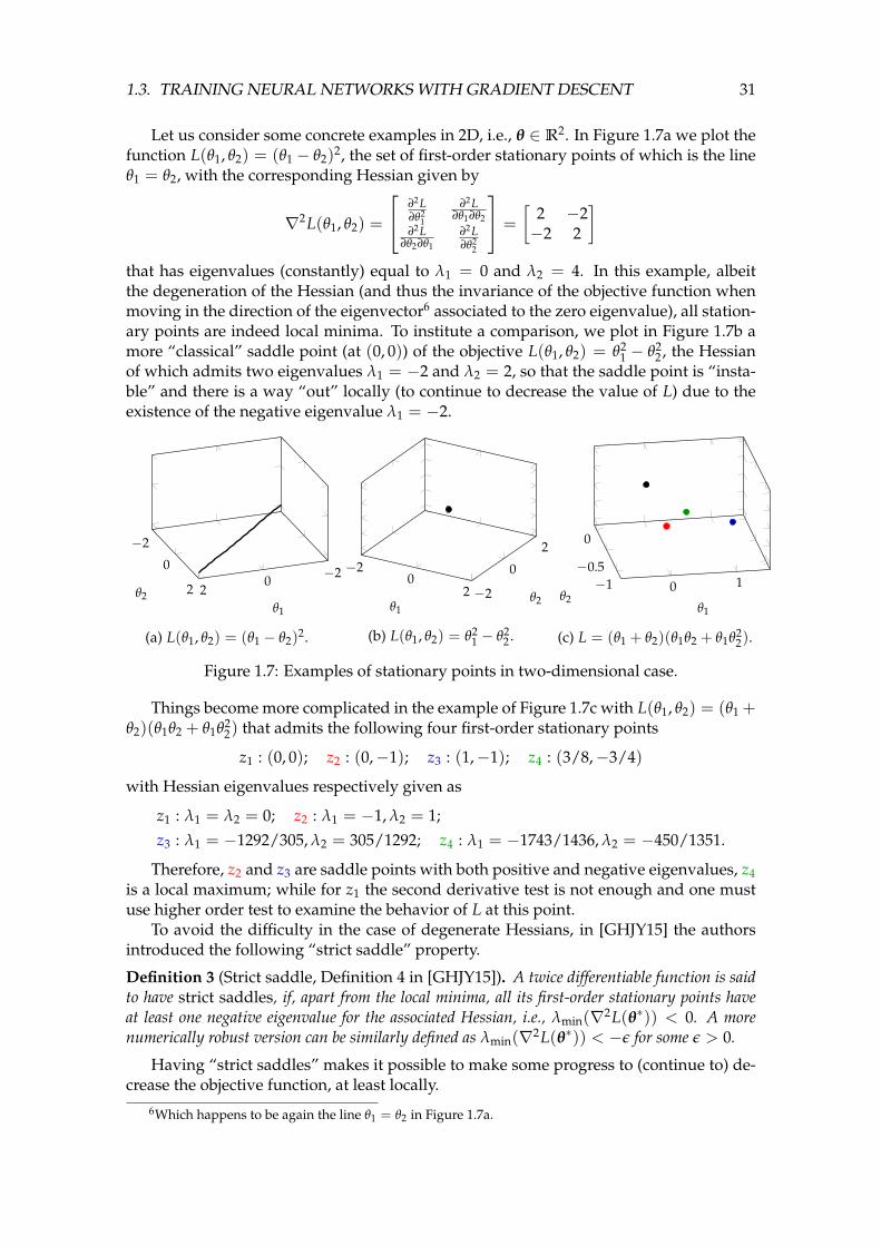
1.3. TRAINING NEURAL NETWORKS WITH GRADIENT DESCENT 31
Let us consider some concrete examples in 2D, i.e., θ ∈ R2. In Figure 1.7a we plot thefunction L(θ1, θ2) = (θ1 − θ2)2, the set of first-order stationary points of which is the lineθ1 = θ2, with the corresponding Hessian given by
∇2L(θ1, θ2) =
∂2L∂θ2
1
∂2L∂θ1∂θ2
∂2L∂θ2∂θ1
∂2L∂θ2
2
=
[2 −2−2 2
]that has eigenvalues (constantly) equal to λ1 = 0 and λ2 = 4. In this example, albeitthe degeneration of the Hessian (and thus the invariance of the objective function whenmoving in the direction of the eigenvector6 associated to the zero eigenvalue), all station-ary points are indeed local minima. To institute a comparison, we plot in Figure 1.7b amore “classical” saddle point (at (0, 0)) of the objective L(θ1, θ2) = θ2
1 − θ22 , the Hessian
of which admits two eigenvalues λ1 = −2 and λ2 = 2, so that the saddle point is “insta-ble” and there is a way “out” locally (to continue to decrease the value of L) due to theexistence of the negative eigenvalue λ1 = −2.
−20
2
−2
0
2θ1
θ2
(a) L(θ1, θ2) = (θ1 − θ2)2.
−20
2 −2
0
2
θ1θ2
(b) L(θ1, θ2) = θ21 − θ2
2 .
0 1−1−0.5
0
θ1θ2
(c) L = (θ1 + θ2)(θ1θ2 + θ1θ22).
Figure 1.7: Examples of stationary points in two-dimensional case.
Things become more complicated in the example of Figure 1.7c with L(θ1, θ2) = (θ1 +θ2)(θ1θ2 + θ1θ2
2) that admits the following four first-order stationary points
z1 : (0, 0); z2 : (0,−1); z3 : (1,−1); z4 : (3/8,−3/4)
with Hessian eigenvalues respectively given as
z1 : λ1 = λ2 = 0; z2 : λ1 = −1, λ2 = 1;z3 : λ1 = −1292/305, λ2 = 305/1292; z4 : λ1 = −1743/1436, λ2 = −450/1351.
Therefore, z2 and z3 are saddle points with both positive and negative eigenvalues, z4is a local maximum; while for z1 the second derivative test is not enough and one mustuse higher order test to examine the behavior of L at this point.
To avoid the difficulty in the case of degenerate Hessians, in [GHJY15] the authorsintroduced the following “strict saddle” property.
Definition 3 (Strict saddle, Definition 4 in [GHJY15]). A twice differentiable function is saidto have strict saddles, if, apart from the local minima, all its first-order stationary points haveat least one negative eigenvalue for the associated Hessian, i.e., λmin(∇2L(θ∗)) < 0. A morenumerically robust version can be similarly defined as λmin(∇2L(θ∗)) < −ε for some ε > 0.
Having “strict saddles” makes it possible to make some progress to (continue to) de-crease the objective function, at least locally.
6Which happens to be again the line θ1 = θ2 in Figure 1.7a.

32 CHAPTER 1. INTRODUCTION
Global min
“Bad” local min
“Good” local min
x
L(x)
Figure 1.8: Examples of different local minima.
Global guarantee of non-convex optimization. Until now, we have been focusing onthe local image of the optimization landscape, which is unfortunately far from our initialgoal of achieving a global minimum. Indeed, if the “strict saddle” property is satisfied, itis possible for gradient-based algorithm to (locally) escape from saddle points and con-tinue to decrease the loss function. Nonetheless, it may still get stuck in a local minimum.Different from the convex case in Figure 1.7a, where the convex (but not strictly convex)objective function L(θ1, θ2) = (θ1 − θ2)2 has a connected region of local (and global) min-ima: θ1 = θ2, a non-convex loss function L may have many “isolated” local minimumregions that are separated by higher values of the loss L. Among these regions, someare desired global minima that reach the smallest possible loss Lmin and some are “bad”local minima that have much greater loss values than Lmin. There may also exist “good”local minima with a relatively small loss but still slightly larger than Lmin and can beconsidered satisfying solutions of the minimization, as illustrated in Figure 1.8.
The isolation between local minimum regions creates many “local valleys” of the losslandscape. Very interestingly, there are both empirical evidence [DVSH18, GIP+18] andtheoretical arguments [FB16] stating that in modern DNNs, most of these “local valleys”are essentially “connected”: i.e., it is possible to construct continuous paths that connect allthese local minimum regions, along which the loss L remains very close to Lmin, as shownin Figure 1.9 (which could be considered a possible 2D representation of Figure 1.8).
Figure 1.9: Minimum energy path (left) and associated loss value (right) in [DVSH18,Figure 1].
Consider now the (more ideal) case that all local minima (connected or isolated) haveexactly the same loss value. This means that for the optimization problem under study,

1.3. TRAINING NEURAL NETWORKS WITH GRADIENT DESCENT 33
all local minima are global. This rules out the presence of “bad” local minima which, to-gether with the strict saddle points property in Definition 3, makes it possible for simplegradient-based algorithms (such as GD or SGD) to achieve a global convergence with aguaranteed rate.
To sum up, the key to handle many non-convex optimization problems is to have both
1. a nice local property: for example the “strict saddle” property in Definition 3;
2. some global guarantee: for instance the “all local minima are global” property.
Although seemingly restrictive, both properties are actually satisfied (under some di-mensionality condition and at least with high probability) by many non-convex opti-mization problems of considerable practical interest: many low rank problems includ-ing matrix sensing, phase retrieval, matrix completion, robust PCA and many others[GJZ17, CLC18].
In the particular case of neural networks, it was shown in [BH89] that for single-hidden-layer linear NNs with square loss and under some dimensionality condition, alllocal minima are essentially global and there is no local maximum (the rest are all sad-dle points). This result was then extended to deep linear NNs in [Kaw16] in which theauthor showed that the same conclusion holds for DNNs with arbitrary H ≥ 1 hiddenlayers. Perhaps more importantly, a necessary condition (on the rank on the weight ma-trix product) was given in [Kaw16] to ensure the associated Hessian have at least onenegative eigenvalue [Kaw16, Theorem 2.3]. This implies the existence of saddle pointswith positive semidefinite Hessian, for which higher order derivatives will be indispens-able for a thorough understanding of these (first-order) stationary points. More precisely,single-hidden-layer (H = 1) linear NN models are proven to have strict saddles, whichis used for instance in [LSJR16] to show almost sure (with respect to the initialization ina Lebesgue measure sense) convergence to global minima in this case; while for H ≥ 2 acounterexample was provided in [Kaw16].
We focus in this manuscript on the gradient flow, for linear NN models in the follow-ing contribution.
(J4) Yacine Chitour, Zhenyu Liao, and Romain Couillet. A geometric approach ofgradient descent algorithms in neural networks. (Submitted to) Journal of Differ-ential Equations, 2019.
Based on a cornerstone “invariance” in the parameter/network weights space in-duced by the network cascading structure, we prove the existence for all time of trajec-tories associated with gradient descent algorithms in linear networks with an arbitrarynumber of layers and the convergence of these trajectories to first order stationary pointsof the loss function. We also prove the exponential/linear convergence of trajectories un-der an extra condition on their initializations. We propose alternative proof of the “almostsure convergence to global minima” fact in single-hidden-layer linear NN model, whichholds true without the technical and unrealistic assumptions demanded in [LSJR16].
1.3.3 Summary of Section 1.3
In this section, we discussed the optimization perspective of large dimensional machinelearning problems, and in particular, NN models trained with gradient descent meth-ods. In Section 1.3.1, inspired by recent advances in [SMG13, AS17], we introduced a

34 CHAPTER 1. INTRODUCTION
RMT-based analysis framework to investigate the GDDs in a linear convex NN modelunder a GMM (see Definition 1) for the input feature. We found a huge gap between thetraining and test performances of the least-square solution when the number of param-eters gets close to the number of training data, that can be efficiently reduced with theearly stopping strategy. This suggests that the use of gradient descent plays an importantrole in regularizing the least-square solution, and sheds new light on the training of largedimensional learning systems.
In Section 1.3.2 we recalled the preliminary local descriptions of (first-order) station-ary points in the general context of differentiable programming, with a particular focuson non-convex optimization. We saw that, if both conditions of “strict saddles” and “alllocal are global” are met, simple gradient-based algorithms such as GD or SGD can ben-efit from a global convergence to global minima, from almost all initializations. It ismoreover possible to speed up the convergence, if the underlying non-convex problem isknown to have some nice (statistical) structure, by properly initializing (often with spec-tral methods) the descent algorithm within some locally convex valley: we will comeback to this point in Chapter 5.
1.4 Outline and Contributions
As stated in the previous sections, this manuscript covers both a “structural” viewpointof large random kernel matrices and neural networks by considering their eigenspectrumbehavior, as well as the “dynamical” optimization aspect of learning in neural networksby means of the corresponding gradient descent dynamics. As a first major contribution,we study the eigenspectrum properties of these large nonlinear learning systems, undera multivariate mixture model (see Definition 1) for the input feature, so as to examinethe subtle yet crucial interplay between the nonlinearity (of the kernel function f , thenonlinear activation σ and the loss function L), the feature statistics (limited to first andsecond here but is envisioned to go well beyond, see our arguments in Remark 1.3 and 2.5later in Section 2.2.2) as well as the problem dimensionality. The second main contribu-tion is the characterization of the gradient descent dynamics (GDDs) in learning bothzero- and single-hidden-layer linear NN models, which opens the door to a more generalRMT-based consideration of non-convex optimization problems.
The remainder of the manuscript is organized as follows. In Chapter 2 we intro-duce the mathematical framework of random matrix theory, with helpful preliminarieson linear algebra, probability theory, and complex analysis. In Chapter 3, we start thediscussion of large random kernel matrices with the concrete example of kernel ridge re-gression, or equivalently least squares support vector machines (LS-SVMs), which servesas the cornerstone of subsequent models such as random feature-based methods andrandom NNs. We will also briefly mention the additional tool needed in handling im-plicit (convex) optimization problems (e.g., logistic regression) that are technically moreinvolved. Then in Chapter 4, random matrix techniques are combined with ideas fromdynamical systems to study the gradient descent dynamics in training simple NNs, firstfrom a statistical standpoint without hidden layer (i.e., linear regression model) and thenwith a “geometric” approach to deal with the extra hidden layers in linear networks. InChapter 5 we provide a quick summary of this manuscript, and perhaps more impor-tantly, discuss some possible limitations of the presented results and eventually somefuture perspectives within the general context of large dimensional machine learning.
We start with the analysis of the classification performance of kernel ridge regression

1.4. OUTLINE AND CONTRIBUTIONS 35
(or LS-SVM) in Section 3.1.1, which helps understand the counterintuitive behavior ofkernel matrices for large dimensional data discussed in Section 1.1.2. Based on a GMMfor the input data (see again Definition 1), we show that, for any locally twice differen-tiable function f , the soft decision function of the kernel ridge regression is asymptoti-cally normally distributed, the mean and variance of which depend on the statistics ofmixture model (µa, Ca), the dimensionality and the function f in a local manner. Thistheoretical result leads to a novel understanding of the negative impact of imbalanceddata in LS-SVM classification and shows an unexpectedly close match when applied onpopular image classification datasets. This finding was first reported in
(C1) Zhenyu Liao and Romain Couillet. Random matrices meet machine learning: alarge dimensional analysis of LS-SVM. In 2017 IEEE International Conference on Acous-tics, Speech and Signal Processing (ICASSP), pages 2397–2401. 2017.
and then with more discussions and detailed proofs in
(J1) Zhenyu Liao and Romain Couillet. A large dimensional analysis of least squaressupport vector machines. IEEE Transactions on Signal Processing, 67(4):1065–1074,2019.
The theoretical analysis of LS-SVM presented above are essentially built upon a lo-cal expansion of the nonlinearity, which is only possible when the similarity measuresunder study (‖xi − xj‖2/p or xTi xj/p) establish a “concentration” around a single pointof the nonlinear function f . With a more natural
√p scaling, one results in the inner-
product kernel that takes the form Kij = f (xTi xj/√
p)/√
p. Very interestingly, the eigen-spectrum of K is shown to only depend on three scalar parameters of the possibly non-differentiable f . This finding is discussed at length in Section 3.1.2 and reported in
(C2) Zhenyu Liao and Romain Couillet. Inner-product kernels are asymptotically equiv-alent to binary discrete kernels, 2019.
Section 3.2 begins with the discussion on single-hidden-layer random weights NN,or equivalently the random feature-based ridge regression in Figure 1.3. For compara-bly large n, p, N, we show that for all dimension-free Lipschitz nonlinear activation σ(·),the random Gram matrix G ≡ 1
n ΣTΣ has an asymptotically tractable behavior, that de-pends solely on σ via the associated underlying kernel K ≡ Ew[σ(XTw)σ(wTX)] for w ∼N (0, Ip). As a consequence, the training MSE can be shown to have an asymptotically(data-dependent) deterministic behavior, with a conjecture provided for the test MSE(and confirmed later in [LC18b]). This work, discussed in more detail in Section 3.2.1, ledto the following publication.
(J2) Cosme Louart, Zhenyu Liao, Romain Couillet. A random matrix approach to neu-ral networks. The Annals of Applied Probability, 28(2):1190–1248, 2018.
In pursuit of a more explicit recognition of the mechanism of different nonlinear ac-tivations, we examine the eigenspectrum of the underlying kernel K, by additionallyleveraging the stochastic nature of the data (that are assumed to follow a GMM). Weshow that, depending on whether the first order (µa), or second order (Ca) informationor both, are conserved after the application of both the random weights W and the entry-wise nonlinearity σ(·). As briefly discussed in Section 1.2.2, commonly used activationsare divided into three categories of mean-oriented, covariance-oriented and balanced.This result, discussed in Section 3.2.2, led to the following contribution.

36 CHAPTER 1. INTRODUCTION
(C3) Zhenyu Liao and Romain Couillet. On the spectrum of random features maps ofhigh dimensional data. In Proceedings of the 35th International Conference on MachineLearning, volume 80, pages 3063–3071. PMLR, 2018.
In Section 3.3 we consider the more generic (and more involved) convex losses (ratherthan the squares loss treated in Section 3.2.1 that conducts to explicit solutions) in a mix-ture classification context and focus mainly on the technical ingredients needed to handleimplicit and highly dependent learning systems. This work was reported in ICASSP 2019with a journal version recently submitted to IEEE Transactions on Signal Processing.
(C4) Xiaoyi Mai, Zhenyu Liao, and Romain Couillet. A large scale analysis of logistic re-gression: Asymptotic performance and new insights. In 2019 IEEE InternationalConference on Acoustics, Speech and Signal Processing (ICASSP), pages 3357–3361.IEEE, 2019.
(J3) Xiaoyi Mai and Zhenyu Liao. High dimensional classification via empirical riskminimization: Improvements and optimality. 2019.
As regards gradient decent dynamics (GDDs) in NN models, we begin in Section 4.1with the discussion on a statistical approach of evaluating the GDD in simple neuralnetworks. Based on a toy mixture model for the input feature, we retrieve, in the highdimensional regime, the (asymptotic) training and test risks of a linear regression model,as a function of the GD training time. From a methodological standpoint, we introducea RMT-based framework (Cauchy’s integral formula + deterministic equivalent) to ex-amine GDDs of simple NN models, which can be reexpressed as some functional of thefeature sample covariance matrix. As a byproduct, we prove for the first time the exis-tence of a “phase-transition” singularity in Figure 1.5, in a high dimensional classificationcontext. This result was first announced in
(C5) Zhenyu Liao and Romain Couillet. The dynamics of learning: a random matrixapproach. In Proceedings of the 35th International Conference on Machine Learning,volume 80, pages 3072–3081. PMLR, 2018.
In Section 4.2 we consider a geometric aspect of GDDs in single-hidden-layer linearNN models. By precisely evaluating the (union of) basin of attraction of all saddle points,we show that almost all initializations lead to an (equivalent) global minimum for thesimplest gradient descent algorithm. Most importantly, this is true without additionalassumptions on these stationary points (e.g., on the gradient norms during descent ortheir Hessians). Indeed, this “global convergence to global minima” conclusion essen-tially holds due to a key invariant structure (in the network weight space) during thegradient descent procedure imposed by the network cascading structure. As a practi-cal outcome, we also derive critical initialization schemes with exponential convergencerate. These results are summarized in
(J4) Yacine Chitour, Zhenyu Liao, and Romain Couillet. A geometric approach of gra-dient descent algorithms in neural networks. 2019.
now under review for Journal of Differentiable Equation, which concludes the Chapter 4.
In Chapter 5 we draw a speedy conclusion of the manuscript and mention some pos-sible limitations of the presented theoretical results, which are admittedly below the per-formance of state-of-the-art models in modern machine learning problems today. We willalso discuss some possible future research directions, in the continuation of our prelimi-nary findings presented here.
Chapter 2
Mathematical Background: RandomMatrix Theory
Random matrix theory, at its inception, primarily dealt with the eigenvalue distribution(also referred to as spectral measure) of large random matrices. One of the key technicaltools to study these measures is the Stieltjes transform, often presented as the centralobject of the theory [BS10].
But signal processing and machine learning alike are more fundamentally interestedin subspaces and eigenvectors (which often carry the structural data information) than ineigenvalues of random matrices. Subspace or spectral methods, such as principal com-ponent analysis (PCA) [WEG87], spectral clustering [NJW02] and some semi-supervisedlearning techniques [Zhu05] are built directly upon the eigenspace spanned by the sev-eral top eigenvectors.
Consequently, beyond the Stieltjes transform, a more general object, the resolvent oflarge random matrices will constitute the cornerstone of this manuscript. The resolvent ofa matrix gives access to its spectral measure, to the location of its isolated eigenvalues, tothe statistical behavior of their associated eigenvectors when random, and consequentlyprovides an entry-door to the performance analysis of numerous learning methods.
2.1 Fundamental Objects
2.1.1 The resolvent
We first introduce the resolvent of a matrix.
Definition 4 (Resolvent). For a symmetric matrix M ∈ Rn×n, the resolvent QM(z) of M isdefined, for z ∈ C not an eigenvalue of M, as
QM(z) ≡ (M− zIn)−1 (2.1)
which is also denoted Q when there is not ambiguity.
Although our focus here will exclusively be on resolvents of (random) matrices, itmust be noted that the resolvent operator is in fact a very classical tool in the analysis oflinear operators in general Hilbert spaces [AG13] as well as in monotone operator theoryof importance to modern convex optimization theory [BC11].
37

38 CHAPTER 2. MATHEMATICAL BACKGROUND: RANDOM MATRIX THEORY
2.1.2 Spectral measure and the Stieltjes transform
The first use of the resolvent QM is in its relation to the empirical spectral measure µM of asquare matrix M, through the Stieltjes transform mµM , which we all define next.
Definition 5 (Empirical spectral measure). For a symmetric matrix M ∈ Rn×n, the spectralmeasure or empirical spectral measure or empirical spectral distribution µM of M is definedas the normalized counting measure of the eigenvalues λ1(M), . . . , λn(M) of M,
µM(x) ≡ 1n
n
∑i=1
δλi(M)(x). (2.2)
Since µM(x) ≥ 0 for all x ∈ R and∫
RµM(x)dx = 1, the spectral measure µM of a
matrix M ∈ Rn×n (random or not) is a probability measure. For (probability) measures,we can define their associated Stieltjes transforms as follows.
Definition 6 (Stieltjes transform). For a real probability measure µ with support supp(µ), theStieltjes transform mµ(z) is defined, for all z ∈ C \ supp(µ), as
mµ(z) ≡∫
R
1t− z
dµ(t). (2.3)
The Stieltjes transform mµ has numerous interesting properties: it is complex analyticon its domain of definition C \ supp(µ), it is bounded by |mµ(z)|dist(z, supp(µ)) ≤ 1,it satisfies =[z] > 0 ⇒ =[m(z)] > 0, and it is an increasing function on all connectedcomponents of its restriction to R \ supp(µ) (since m′µ(x) =
∫R(t − x)−2dt > 0) with
limx→±∞ mµ(x) = 0 if supp(µ) is bounded.As a transform, mµ admits an inverse formula to recover µ, as per the following result.
Theorem 2.1 (Inverse Stieltjes transform). For a, b continuity points of the probability measureµ, we have
µ([a, b]) =1π
limy↓0
∫ b
a=[mµ(x + ıy)
]dx. (2.4)
Besides, if µ admits a density f at x, i.e., µ(x) is differentiable in a neighborhood of x and
limε→0
(2ε)−1µ([x− ε, x + ε]) = f (x)
thenf (x) =
1π
limy↓0=[mµ(x + ıy)
]. (2.5)
Finally, if µ has an isolated mass at x, then
µ(x) = − 1π
limy↓0
ıymµ(x + ıy). (2.6)
Proof. Since | y(t−x)2+y2 | ≤ 1
y for y > 0, by Fubini’s theorem,
1π
∫ b
a=[mµ(x + ıy)
]dx =
1π
∫ b
a
[∫R
y(t− x)2 + y2 dµ(t)
]dx
=1π
∫R
[∫ b
a
y(t− x)2 + y2 dx
]dµ(t)
=1π
∫R
[arctan
(b− t
y
)− arctan
(a− t
y
)]dµ(t).
2.1. FUNDAMENTAL OBJECTS 39
As y ↓ 0, the difference in brackets converges either to ±π or 0 depending on the relativeposition of a, b, t. By the dominated convergence theorem, limits and integrals can beexchanged, and the limit, as y ↓ 0, is
∫R
1[a,b]dµ(t) = µ([a, b]).
The important relation between the spectral measure of M ∈ Rn×n, the Stieltjes trans-form mµM(z) and the resolvent QM lies in the fact that
mµM(z) =1n
n
∑i=1
∫R
δλi(M)(t)t− z
=1n
n
∑i=1
1λi(M)− z
=1n
tr(QM). (2.7)
Combining inverse Stieltjes transform and the relation above thus provides a linkbetween QM and the eigenvalue distribution of M. While seemingly contorted, this linkis in general the only efficient way to study the spectral measure of large dimensionalrandom matrices M.
Remark 2.1 (Resolvent as a matrix-valued Stieltjes transform). As proposed in [HLN07],it can be convenient to extrapolate Definition 6 of Stieltjes transforms to n × n matrix-valuedpositive measures M(dt),1 in which case Equation (2.7) can be generalized as
QM(z) =∫
R
M(dt)t− z
= U diag
1λi(M)− z
n
i=1UT
where we used the spectral decomposition M = U diagλi(M)ni=1UT. In particular, QM(z) en-
joys similar properties as Stieltjes transforms of real-valued measures: ‖QM(z)‖ ≤ dist(z, supp(µM))−1,and x 7→ QM(x) for x ∈ R \ supp(µ) is an increasing matrix-valued function with respect tosymmetric matrix partial ordering (i.e., A B whenever zT(A− B)z ≥ 0 for all z).
2.1.3 Cauchy’s integral, linear eigenvalue functionals, and eigenspaces
Being complex analytic, the resolvent QM can be manipulated using advanced tools fromcomplex analysis. Of particular interest to spectrum-based machine learning methods isthe relation between the resolvent and Cauchy’s integral theorem.
Theorem 2.2 (Cauchy’s integral formula). For Γ ∈ C a positively (i.e., counterclockwise)oriented simple closed curve and a complex function f (z) analytic in a region containing Γ andits interior, then
1) if z0 ∈ C is enclosed by Γ, f (z0) = − 12πı
∮Γ
f (z)z0−z dz;
2) if not, 12πı
∮Γ
f (z)z−z0
dz = 0.
This result provides an immediate link between the linear functionals of the eigenvaluesof M and the Stieltjes transform through
1n
n
∑i=1
f (λi(M)) = − 12πın
∮Γ
f (z) tr(QM(z))dz = − 12πı
∮Γ
f (z)mµM(z)dz
for all f complex analytic in a compact neighborhood of supp(µM), by choosing the con-tour Γ to enclose supp(µM) (i.e., all the λi(M)’s). More generally,
1n ∑
λi(M)∈Γf (λi(M)) = − 1
2πı
∮Γ
f (z)mµM(z)dz
1Defined by the fact that µ(dt; z) = zTM(dt)z = ∑ij zizjMij(dt) is a positive real-valued measure for allz. See [RRR67] for an introduction.

40 CHAPTER 2. MATHEMATICAL BACKGROUND: RANDOM MATRIX THEORY
for Γ the interior of contour Γ.
Another quantity of interest relates to eigenvectors and eigenspaces. Decomposingthe symmetric matrix M = UΛUT in its spectral decomposition with U = [u1, . . . , un] ∈Rn×n and Λ = diag(λ1(M), . . . , λn(M)), we have
QM(z) =n
∑i=1
uiuTi
λi(M)− z
and thus the direct access to the i-th eigenvector of M through
uiuTi = − 1
2πı
∮Γλi(M)
QM(z)dz
for Γλi(M) a contour circling around λi(M) only (if λi(M) is of unit multiplicity). Moregenerally,
U f (Λ; Γ)UT = − 12πı
∮Γ
f (z)QM(z)dz
for f analytic in a neighborhood of Γ and its interior and f (Λ; Γ) = diag( f (λi(M))1λi(M)∈Γni=1).
Of interest in this manuscript will be the projection of the individual eigenvectors uiof M onto a deterministic eigenvector v. In particular, from the above,
|vTui|2 = − 12πı
∮Γλi(M)
vTQM(z)vdz.
It is important to note that the resolvent provides access to scalar observations of theeigenstructure of M through linear functionals of the resolvent M, i.e., the scalar observa-tions 1
n ∑i f (λi(M)) and |vTui| accessible from tr QM and vTQMv, respectively.
2.1.4 Deterministic and random equivalents
This manuscript is concerned with the situation where M is a large dimensional randommatrix, the eigenvalues and eigenvectors of which need be related to the statistical natureof the model design of M.
In the early days of random matrix theory, the main focus was on the limiting spectralmeasure of M, that is the characterization of a certain “limit” to the spectral measureµM of M as the size of M increases. To this purpose, the natural approach is to studythe random Stieltjes transform mµM(z) and to show that is admits a deterministic limit(in probability or almost surely) m(z). However, this method shows strong limitationstoday: i) it supposes that such a limit does exist, therefore restricting the study to veryisotropic models for M and ii) it only quantifies tr QM (through the Stieltjes transform),thereby discarding all subspace information about M carried in QM (as a consequence, afurther study of the eigenvectors of M requires a complete rework).
To avoid these limitations, modern random matrix theory uses the notion of determin-istic equivalents which are non-asymptotic deterministic matrices having (in probability oralmost surely) asymptotically the same scalar observations as the random ones.
Definition 7 (Deterministic Equivalent). We say that Q ∈ Rn×n is a deterministic equivalentfor the symmetric random matrix Q ∈ Rn×n if, for (sequences of) deterministic matrix A ∈ Rn×n
and vectors a, b ∈ Rn of unit norms (operator and Euclidean, respectively), we have, as n→ ∞,
1n
tr A(Q− Q)→ 0, aT(Q− Q)b→ 0
where the convergence is either in probability or almost surely.

2.2. FOUNDATIONAL RANDOM MATRIX RESULTS 41
This definition has the advantage to bring forth the two key elements giving access tospectral information about a random matrix M: traces and bilinear forms (of its resolventQM(z) for some z). Deterministic equivalents of resolvents QM then encode most of theinformation necessary to statistically quantify a random matrix M.
A practical use of deterministic equivalents is to establish that, for a random matrixM, 1
n tr(QM(z)− Q(z)) → 0, say almost surely, for all z ∈ C with C ⊂ C some region ofC. Denoting mn(z) = 1
n tr Q(z), this convergence implies that the Stieltjes transform ofµM “converges” in the sense that mµM(z)− mn(z) → 0. As we will see, this will indicatethat µM gets increasingly well approximated by a probability measure µn having Stieltjestransform mn(z). Identifying mn(z), which uniquely defines µn, will often be as far as theStieltjes transform method will lead us. But in some rare cases (such as with the Marcenko-Pastur and the semi-circle laws), µn will be explicitly identifiable.
In the remainder of the manuscript, we will often characterize the large dimensionalbehavior of random matrix models M through an approximation by deterministic equiv-alents Q(z) of their associated resolvents QM(z), as this offers access not only to theirasymptotic spectral measure but also to their eigenspaces. We shall therefore often ex-trapolate some of the traditional results, such as the Marcenko–Pastur law [MP67], thesample covariance matrix model [SB95], etc., under this more general form.
Remark 2.2 (Q versus EQ). For Q a deterministic equivalent for Q, the probabilistic conver-gences 1
n tr A(Q− Q)→ 0 and aT(Q− Q)b→ 0 will in general unfold from the fact that
‖EQ− Q‖ → 0
and from a control of the variance of 1n tr(AQ) and aTQb; this will often be the strategy fol-
lowed in our proofs. But note importantly that, if the above relation is met, then EQ itself is adeterministic equivalent for Q by Definition 7. However, EQ is often not convenient to workwith and a “truly” deterministic matrix Q involving no integration over probability spaces willbe systematically preferred.
In some situations, deterministic equivalents may either not exist or, as will often bethe case, will only be reachable through the access to an intermediary random matrix. Tosimplify the readability of the main results and proofs in the remainder of the manuscript,which involve both deterministic and random equivalents, we introduce the followingshortcut notation.
Notation 1 (Deterministic and Random Equivalents). For X, Y ∈ Rn×n two random ordeterministic matrices, we write
X↔ Y
if, for all A ∈ Rn×n and a, b ∈ Rn of unit norms (respectively, operator and Euclidean), we havethe simultaneous results
1n
tr A(X− Y) a.s.−→0, aT(X− Y)b a.s.−→0, ‖E[X− Y]‖ → 0.
2.2 Foundational Random Matrix Results
In this section we introduce the main historical results of random matrix theory (appro-priately updated under a deterministic equivalent form), which will serve as supporting

42 CHAPTER 2. MATHEMATICAL BACKGROUND: RANDOM MATRIX THEORY
models to most applications to machine learning. For readability and accessibility to thereaders new to random matrix theory, we mostly stick to intuitive and short sketches ofproofs. Yet, for the readers to have a glimpse on the technical details and modern tools ofthe field, some of the proof sketches will be appended by a complete exhaustive proof.
Both sketches and detailed proofs rely on a set of elementary lemmas and identitieswill be introduced below in Section 2.2.1. The main difference between sketches anddetailed proofs then relies on additional technical probability theory arguments to provevarious convergence results. These arguments strongly depend on the underlying ran-dom matrix model hypotheses (Gaussian independent, i.i.d., concentrated random vec-tors, etc.); for readability, we will focus in our proofs on one specific line of proof (thatwe claim to be the “historical” one) and will introduce some side remarks concerningalternative approaches.
2.2.1 Key lemmas and identities
Resolvent identities
Most results discussed in this section consist in approximating random resolvents Q(z)via deterministic resolvents Q(z), which are both inverse of matrices. The following firstidentity provides a comparison of inverse matrices.
Lemma 2.1 (Resolvent identity). For invertible matrices A and B, we have
A−1 − B−1 = A−1(B−A)B−1.
Proof. This can be easily checked by multiplying both sides on the left by A and on theright by B.
Another useful lemma that helps directly connect the resolvent of BA to that of AB,is given as follows.
Lemma 2.2. For A ∈ Rp×n and B ∈ Rn×p , we have
A(BA− zIn)−1 = (AB− zIp)
−1A
for z ∈ C distinct from 0 and from the eigenvalues of AB.
For AB and BA symmetric, Lemma 2.2 is a special case of the more general rela-tion A f (BA) = f (AB)A, with f (M) ≡ U f (Λ)UT under the spectral decompositionM = UΛUT and f complex analytic. Since f is analytic, f (BA) = ∑∞
i=0 ci(BA)i for somesequence ci∞
i=0 and thus A f (BA) = ∑∞i=0 ci(AB)iA = f (AB)A.
The next lemma, known as Sylvester’s identity, similarly relates the resolvents of ABand BA through their determinant.
Lemma 2.3 (Sylvester’s identity). For A ∈ Rp×n, B ∈ Rn×p and z ∈ C,
det(AB− zIp
)= det (BA− zIn) (−z)p−n.
An immediate consequence of Sylvester’s identity is that AB and BA have the samenon-zero eigenvalues (those non-zero z’s for which both left- and right-hand sides vanish).Thus, say n ≥ p, AB ∈ Rp×p and BA ∈ Rn×n have the same spectrum, except for theadditional n− p zero eigenvalues of AB. This remark implies the next identity.

2.2. FOUNDATIONAL RANDOM MATRIX RESULTS 43
Lemma 2.4 (Trace of resolvent and co-resolvent). Let A ∈ Rp×n, B ∈ Rn×p, and z ∈ C notan eigenvalue of AB nor zero. Then
tr QAB(z) = tr QBA(z) +n− p
z.
In particular, if AB and BA are symmetric,
mµAB(z) =np
mµBA(z) +n− p
pz.
Perturbation identities
Quantifying the asymptotic global (e.g., spectral distribution) or local (e.g., isolated eigen-values or projection on eigenvector) behavior of random matrices M will systematicallyinvolve a perturbation approach. The idea often lies in comparing the behavior of the resol-vent Q = QM to the resolvent Q−i of M−i, with M−i defined as M with either row andcolumn i, or some i-th contribution (e.g., M−i = ∑j 6=i xjxTj if M = ∑j xjxTj ), discarded. Anumber of so-called perturbation identities are then needed.
The first one involves the segmentation of M under the form of sub-blocks, in gen-eral consisting of one large block and three small sub-matrices. The resolvent QM cancorrespondingly be segmented in sub-blocks according to the following block inversionlemma.
Lemma 2.5 (Block matrix inversion). For A ∈ Rp×p, B ∈ Rp×n, C ∈ Rn×p and D ∈ Rn×n
with D invertible, we have(A BC D
)−1
=
(S−1 −S−1BD−1
−D−1CS−1 D−1 + D−1CS−1BD−1
)where S ≡ A− BD−1C is the Schur complement (for the block D) of
(A BC D
).2
As a consequence of Lemma 2.5, we have the following explicit form for all diagonalentries of an invertible matrix A.
Lemma 2.6 (Diagonal entries of matrix inverse). For invertible A ∈ Rp×p and A−i ∈R(p−1)×(p−1), the matrix obtained by removing the i-th row and column from A, i = 1, . . . , p,we have
(A−1)ii =1
Aii − αTi (A−i)−1βi
for αTi , βi ∈ Rp−1 the i-th row and column of A with i-th entries removed, respectively.
The result is a direct consequence of the fact that A−1 = adj(A)det(A)
, with adj(A) the adju-gate matrix of A, together with the block determinant formula in Lemma 2.5.
Perturbations by addition or subtraction of low-rank matrices to M induce modifica-tions in the resolvent QM that involve Woodbury’s identity as follows.
Lemma 2.7 (Woodbury). For A ∈ Rp×p, U, V ∈ Rp×n, such that both A and A + UVT areinvertible, we have
(A + UVT)−1 = A−1 −A−1U(In + VTAU)−1VTA−1.2The Schur complement S = A− BD−1C is particularly known for its providing the block determinant
formula det( A B
C D)= det(D)det(S).

44 CHAPTER 2. MATHEMATICAL BACKGROUND: RANDOM MATRIX THEORY
Note importantly that, while (A + UVT)−1 is of size p× p, (In + VAU)−1 is of sizen × n. This will turn out useful to relate resolvents of large dimensional matrices toresolvents of more elementary fixed small size matrices. In particular, for n = 1, i.e.,UVT = uvT for U = u ∈ Rp and V = v ∈ Rp, Woodbury’s identity specializes to theSherman–Morrison formula.
Lemma 2.8 (Sherman–Morrison). For A ∈ Rp×p invertible and u, v ∈ Rp, A + uvT isinvertible if and only if 1 + vTA−1u 6= 0 and
(A + uvT)−1 = A−1 − A−1uvTA−1
1 + vTA−1u.
Besides,
(A + uvT)−1u =A−1u
1 + vTA−1u.
Letting A = M− zIp, z ∈ C, and v = τu for τ ∈ R in the previous lemma leads tothe following rank-1 perturbation lemma for the resolvent of M.
Lemma 2.9 (From Lemma 2.6 in [SB95]). For A, M ∈ Rp×p symmetric, u ∈ Rp, τ ∈ R andz ∈ C \R, ∣∣∣tr A(M + τuuT − zIp)
−1 − tr A(M− zIp)−1∣∣∣ ≤ ‖A‖|=(z)| .
Also, for A, M ∈ Rp×p symmetric and nonnegative definite, u ∈ Rp, τ > 0 and z < 0,∣∣∣tr A(M + τuuT − zIp)−1 − tr A(M− zIp)
−1∣∣∣ ≤ ‖A‖|z| .
It is interesting (and possibly counterintuitive at first) to note that ‖u‖ does not inter-vene in this inequality. In particular, irrespective of the amplitude of the rank-1 pertur-bation, under the conditions of the lemma
mµM+τuuT(z) = mµM(z) + O(p−1)
and thus, by the link between spectrum and Stieltjes transform, the spectral measureof M is asymptotically close to that of M + τuuT for any u, in the large p limit. Thisresult can be understood through the following two arguments: i) for large p, the spec-trum of M (say ‖M‖ = O(1) without generality restriction) is only non-trivial if thevast majority of the p eigenvalues of M are of order O(1): thus, as p eigenvalues use aspace of size O(1), they tend to aggregate; ii) by Weyl’s interlacing lemma presented next(Lemma 2.10) for symmetric matrices, the eigenvalues of M and of M + τuuT are inter-laced. Both arguments thus indicate that, in the large p limit, the spectral measures areindeed asymptotically the same.
Unlike non-symmetric matrices, symmetric matrices indeed enjoy the nice propertyof having stable spectra with respect to rank-1 perturbations. For λ ∈ R an eigenvalue ofM + τuuT but not of M with, say τ > 0, we indeed have
0 = det(M + τuuT − λIp) = det(QM(λ))det(Ip + τQM(λ)uuT)
= det(QM(λ))(
1 + τuTQM(λ)u)

2.2. FOUNDATIONAL RANDOM MATRIX RESULTS 45
where the second equality unfolds from factoring out M− λIp (which is not singular asλ is not an eigenvalue of M) and the third from Sylverster’s identity (Lemma 2.3). As aconsequence, λ is one of the solutions to
−1 = τuTQM(λ)u = τp
∑i=1
|vTi u|2
λi(M)− λ,
(M =
p
∑i=1
λi(M)vivTi
)
which, seen as a function of λ, has asymptotes at each λi(M) and is increasing (from−∞ to ∞) on the segments (λi(M), λi+1(M)) (eigenvalues being sorted in increasing or-der). The eigenvalues of M + τuuT are therefore interlaced with those of M. This ideageneralizes to finite rank perturbation as follows.
Lemma 2.10 (Weyl, Theorem 4.3.1 in [HJ12]). Let A, B ∈ Rp×p be symmetric matrices and letthe respective eigenvalues of A, B and A + B arranged in nondecreasing order, i.e., λ1 ≤ λ2 ≤. . . λp−1 ≤ λp. Then, for all i ∈ 1, . . . , p,
λi(A + B) ≤ λi+j(A) + λp−j(B), j = 0, 1, . . . , p− i,
λi−j+1(A) + λj(B) ≤ λi(A + B), j = 1, . . . , i,
In particular, taking i = 1 in the first equation and i = p in the second inequation, together withthe fact λj(B) = −λp+1−j(−B) for j = 1, . . . , p, implies
max1≤j≤p
|λj(A)− λj(B)| ≤ ‖A− B‖.
Probability identities
The results of the previous sections are algebraic identities allowing for handling theresolvent QM of the deterministic matrix M. The second ingredient of random matrixanalysis lies in asymptotic probability approximations as the dimensions of M increase.Quite surprisingly, most results essentially revolve around the convergence of a certainquadratic form, which is often nothing more than a mere extension of the law of largenumbers.
Those quadratic form convergence results come under multiple forms. The historicalform, due to Bai and Silverstein, sometimes referred to as the “trace lemma”, is as follows.
Lemma 2.11 (Quadratic-form-close-to-the-trace, Lemma B.26 in [BS10]). Let x ∈ Rp havei.i.d. entries of zero mean, unit variance and E[|xi|L] ≤ νL for some L ≥ 1. Then for A ∈ Rp×p
and l ≥ 1
E
[∣∣∣xTAx− tr A∣∣∣l] ≤ Kl
[(ν4 tr(AAT)
)l/2+ ν2l tr(AAT)l/2
]for some constant Kl > 0 independent of p. In particular, if ‖A‖ ≤ 1 and the entries of x havebounded eighth-order moment,
E
[(xTAx− tr A
)4]≤ Kp2
for some K independent of p, and consequently, as p→ ∞,
1p
xTAx− 1p
tr A a.s.−→0.

46 CHAPTER 2. MATHEMATICAL BACKGROUND: RANDOM MATRIX THEORY
This last result is rather intuitive. For A = Ip, this is simply an instance of the lawof large numbers. For generic A, first note that, by the independence of the entries ofx, E[xTAx] = E[tr(AxxT)] = tr A. Exploiting the fact that Var
[1p xTAx
]= O(p−1) then
ensures that 1p xTAx − 1
p tr A → 0, but only in probability; since the variance calculusinvolves exponentiating the entries xi of x to power 4, they need to be of finite fourthpower. The almost sure convergence is achieved by showing the faster moment conver-gence E[( 1
p xTAx− 1p tr A)4] = O(p−2) which is the second statement of the lemma and
requires 8-th order exponentiation of the xi’s. The request for A to be of bounded normwith respect to p in this case “stabilizes” the quadratic form xTAx by maintaining itsrandom concentration properties.
Recalling that ‖QM(z)‖ ≤ (dist(z, supp(µM)))−1, Lemma 2.11 can be exploited forA = QM(z) for all z away from the support of µM and all x independent of QM(z). Thecore of the proofs of the main random matrix results is uniquely based on this last remark.
These identities constitute the main technical ingredients needed to understand theproofs of both historical and recent random matrix results. The next section introducesthe most fundamental of those which will be called after over and over in the remainderof the manuscript.
2.2.2 The Marcenko-Pastur law
We start by illustrating how the aforementioned tools are used to prove one of the mostpopular results in random matrix theory: the Marcenko-Pastur law. Another importantresult is the Wigner semi-circle law, which, despite being popular in many graph-basedproblems, is less covered in the works addressed in this manuscript and thus omitted.
To simplify the exposition of the results, we will use the notation for deterministicequivalents introduced in Notation 1. That is, for X, Y ∈ Rn×n, we will denote X ↔ Yif, for all unit norm A ∈ Rn×n and a, b ∈ Rn, 1
n tr A(X − Y) a.s.−→0, aT(X − Y)b a.s.−→0 and‖E[X− Y]‖ → 0.
Most of the results involve Stieltjes transforms mµ(z) of probability measures withsupport supp(µ). Since Stieltjes transforms are such that mµ(z) > 0 for z < inf supp(µ),mµ(z) < 0 for z > sup supp(µ) and =[z]=[mµ(z)] > 0 if z ∈ C \R, it will be convenientin the following to consider the set
Z(A) =(z, m) ∈ A2, (=[z]=[m] > 0 if =[z] 6= 0) or (zm < 0 if =[z] = 0)
.
We present the Marcenko-Pastur law under the slightly modified form of a determin-istic equivalent for the resolvent Q(z).
Theorem 2.3 (From [MP67]). Consider the resolvent Q(z) = ( 1n XXT − zIp)−1, for X ∈ Rp×n
having i.i.d. zero mean and unit variance entries. Then, as n, p → ∞ with p/n → c ∈ (0, ∞),we have
Q(z)↔ Q(z), Q(z) = m(z)Ip (2.8)
with (z, m(z)) the unique solution in Z(C \ [(1−√
c)2, (1 +√
c)2]) of
zcm2(z)− (1− c− z)m(z) + 1 = 0. (2.9)
The function m(z) is the Stieltjes transform of the probability measure µ given explicitly by
µ(dx) = (1− c−1)+δ(x) +1
2πcx
√(x− a)+(b− x)+dx (2.10)

2.2. FOUNDATIONAL RANDOM MATRIX RESULTS 47
where a = (1−√
c)2, b = (1+√
c)2 and (x)+ = max(0, x), which is known as the Marcenko-Pastur distribution. In particular, with probability one, the empirical spectral measure µ 1
n XXT
converges weakly to µ.
Figure 2.1 depicts the density of the Marcenko-Pastur distribution for different valuesof c. For a fixed dimension p, the ratio c decreases as the number of samples n grows large,so that the eigenvalues of the sample covariance matrix become more “concentrated”(their spread is given by the length of the support [(1 −
√c)2, (1 +
√c)2]) around the
unique population covariance matrix eigenvalue equal to 1.
0 0.5 1 1.5 2 2.5 30
0.2
0.4
0.6
0.8
1
1.2
x
µ
c = 0.1c = 0.2c = 0.5
Figure 2.1: Marcenko-Pastur distribution for different c
Proof. Before going into the details of the proof, we first give a few intuitive arguments.
Intuitive idea. A first heuristic derivation consists in iteratively “guessing” the form ofQ(z) = F(z)−1 for some matrix F(z)−1. To this end, from Lemma 2.1, it first appears that
Q(z)− Q(z) = Q(z)(
F(z) + zIp −1n
XXT
)Q(z)
= Q(z)
(F(z) + zIp −
1n
n
∑i=1
xixTi
)Q(z)
For Q(z) to be a deterministic equivalent for Q(z), we wish in particular that 1p tr A(Q(z)−
Q(z)) a.s.−→0, for A deterministic with ‖A‖ = 1. That is
1p
tr(F(z) + zIp)Q(z)AQ(z)− 1n
n
∑i=1
1p
xTi Q(z)AQ(z)xia.s.−→0. (2.11)
We recognize in 1p xTi Q(z)AQ(z)xi a quadratic form on which we would like to use Lemma 2.11
to turn it into a trace term independent of xi. Yet, Lemma 2.11 cannot be used as Q(z)depends on xi. To counter the difficulty, we then use Lemma 2.8 to write
Q(z)xi =Q−i(z)xi
1 + 1n xTi Q−i(z)xi
48 CHAPTER 2. MATHEMATICAL BACKGROUND: RANDOM MATRIX THEORY
where Q−i(z) = ( 1n ∑j 6=i xjxTj − zIp)−1 is independent of xi. Now legitimately applying
Lemma 2.11, we find that
1p
xTi Q(z)AQ(z)xi =
1p xTi Q(z)AQ−i(z)xi
1 + 1n xTi Q−i(z)xi
'1p tr Q(z)AQ−i(z)
1 + 1n tr Q−i(z)
. (2.12)
From Lemma 2.9, normalized traces involving Q−i(z) or Q(z) are asymptotically identi-cal and thus this further reads
1p
xTi Q(z)AQ(z)xi '1p tr Q(z)AQ(z)
1 + 1n tr Q(z)
.
Getting back to (2.11), we thus end up with the approximation
1p
tr(F(z) + zIp)Q(z)AQ(z) '1p tr Q(z)AQ(z)
1 + 1n tr Q(z)
.
As a consequence, we can now “guess” the form of F(z). Indeed, if it is to exist, F(z)must be of the type
F(z) '(−z +
11 + 1
n tr Q(z)
)Ip
for the approximation above to hold. To close the loop, taking A = Ip, 1n tr Q(z) appear-
ing in this display must be well approximated by m(z) ≡ 1p tr Q(z) so that
1p
tr Q(z) ' m(z) =1
−z + 11+ p
n1p tr Q(z)
' 1−z + 1
1+ pn m(z)
(2.13)
and we thus have finally
Q(z) = F(z)−1 = m(z)Ip
where, in the large n, p limit, m(z) is solution to
m(z) =1
−z + 11+cm(z)
or equivalently
zcm2(z)− (1− c− z)m(z) + 1 = 0.
This equation has two solutions defined by the two roots of the complex square rootfunction
m(z) =1− c− z
2cz+
√((1 +
√c)2 − z)((1−
√c)2 − z)
2cz
only one of which is such that =[z]=[m(z)] > 0 as imposed by the definition of Stieltjestransforms. Now, from the inverse Stieltjes transform theorem, Theorem 2.1, we find thatm(z) is the Stieltjes transform of the measure µ with
µ([a, b]) =1π
limε↓0
∫ b
a=[m(x + ıε)]dx

2.2. FOUNDATIONAL RANDOM MATRIX RESULTS 49
for all continuity points a, b ∈ R of µ. The term under the square root in m(z) being nega-tive only in the set [(1−
√c)2, (1+
√c)2], the latter defines the support of the continuous
part of the measure µ with density√
((1+√
c)2−x)(x−(1−√
c)2)2cπx at point x in the set. The case
x = 0 brings a discontinuity in µ with weight equal to
µ(0) = − limy↓0
ıym(ıy) =c− 1
2c± c− 1
2c
where the sign is established by a second order development of zm(z) in the neighbor-hood of zero.
Detailed proof. Having heuristically identified Q(z), we shall now use sound math-ematical tools to prove that, indeed, Q(z) is a deterministic equivalent for Q(z) in thesense of the theorem statement. Let us first show that E[Q(z)] = Q(z) + o‖·‖(1), whereo‖·‖(1) denotes a matrix term of vanishing operator norm as n, p→ ∞.
Convergence in mean. For mathematical convenience, we will take z < 0 in what follows.Since Q(z) and Q(z) from the theorem statement are complex analytic functions for z /∈R+ (matrix-valued Stieltjes transforms are analytic), obtaining the convergence resultson R− is equivalent to obtaining the result on all of C \R+.
We proceed in two steps by first introducing the intermediate deterministic quantitiesα(z) ≡ 1
n tr E[Q(z)] and ¯Q(z) ≡ (−z + 11+α(z) )
−1Ip. From Lemma 2.1, we have (the
argument z in α(z), Q(z) and ¯Q(z) is dropped when confusion is not possible)
E[Q− ¯Q] = EQ(
Ip
1 + α− 1
nXXT
)¯Q =
E[Q]
1 + α¯Q− 1
nE[QXXT] ¯Q
=E[Q]
1 + α¯Q−
n
∑i=1
1n
E[QxixTi ]¯Q =
E[Q]
1 + α¯Q−
n
∑i=1
E
[Q−i
1n xixTi
1 + 1n xTi Q−ixi
]¯Q
where we applied Lemma 2.8 to obtain the last equality and denoted Q−i ≡ (∑j 6=i1n xjxTj −
zIp)−1 as previously.Since we expect 1
n xTi Q−ixi to be close to α (as a consequence of Lemma 2.11), werewrite
Q−i1n xixTi
1 + 1n xTi Q−ixi
=Q−i
1n xixTi
1 + α−
Q−i1n xixTi (
1n xTi Q−ixi − α)
(1 + α)(1 + 1n xTi Q−ixi)
so that
E[Q− ¯Q] =E[Q]
1 + α¯Q−
n
∑i=1
E[Q−i
1n xixTi
] ¯Q1 + α
+n
∑i=1
E[Q 1
n xixTi di] ¯Q
1 + α
=E[Q]
1 + α¯Q−
n
∑i=1
E[Q−i
1n xixTi
] ¯Q1 + α
+E[Q 1
n XDXT] ¯Q
1 + α
where we introduced D = diagdini=1 for di =
1n xTi Q−ixi− α, and used again Lemma 2.8
to write Q−i1n xixTi
1+ 1n xTi Q−ixi
= Q 1n xixTi in the first equality. Since E[Q−ixixTi ] = E[Q−i], this
further reads
E[Q− ¯Q] =1n
n
∑i=1
(E[Q]−E[Q−i])¯Q
1 + α+
E[ 1
n QXDXT] ¯Q
1 + α.

50 CHAPTER 2. MATHEMATICAL BACKGROUND: RANDOM MATRIX THEORY
Again from Lemma 2.1 and 2.8,
1n
n
∑i=1
E[Q−Q−i] = −1n
n
∑i=1
E
[Q
1n
xixTi Q−i
]= − 1
n
n
∑i=1
E
[Q
1n
xixTi Q(
1 +1n
xTi Q−ixi
)]= − 1
nE
[Q
1n
XD2XTQ]
where D2 = diag
1 + 1n xTi Q−ixi
ni=1 and thus
E[Q− ¯Q] = − 1n
E
[Q
1n
XD2XTQ] ¯Q
1 + α+
E[ 1
n QXDXT] ¯Q
1 + α. (2.14)
It remains to show that the right-hand side terms vanish in the large p, n limit.For the first term, note that
0 Q1n
XD2XTQ Q1n
XXTQ max1≤i≤n
[D2]ii
in the order of symmetric matrices. Since Q 1n XXT = Ip + zQ which is of bounded op-
erator norm, controlling ‖E[Q 1n XD2XTQ]‖ boils down to controlling E[maxi[D2]ii]. This
can be established in various ways. From the union bound and the i.i.d. nature of the xi’s,
P(
maxi
[D2]ii > t)≤ nP ([D2]11 > t) .
Now, by Markov’s inequality P(X > a) ≤ E[Xk]/ak for every k (for X, a > 0) and themoment inequality in Lemma 2.11 for, say l = 4, P(maxi[D2]ii > t) may be boundedby a function decreasing as t−2, for all t > 1 + α(z), and of order n−1. Since E[X] =∫
X>0 P(X > t)dt, we then find that E[maxi[D2]ii] is bounded. Alternatively, one mayhave used a concentration inequality argument to show the same. Consequently, due tothe leading 1/n factor in front of the first right-hand side term of (2.14), this term vanishesas n, p→ ∞.
To handle the second right-hand side term in (2.14), one needs to control the normof 1
n QXDXT ¯Q. This is not a symmetric matrix, but E[Q − ¯Q] is. We may thus rewrite(2.14) as the half-sum of itself and its transpose and we are thus left to controlling theoperator norm of 1
n QXDXT ¯Q+ 1n
¯QXDXTQ. Using the matrix inequalities ABT+BAT AAT + BBT (from (A− B)(A− B)T 0) and ABT + BAT −AAT − BBT (from (A +B)(A + B)T 0), we are left to bounding the norm of
E
[1
n√
nQXXTQ
]+ E
[1√n
¯QXD2XT ¯Q]
where the division of the 1/n2 term into 1/(n√
n) and 1/√
n is essential. The first termabove is easily seen to be of order 1/
√n. As for the second, using as above the moment
inequality in Lemma 2.11 along with Markov’s inequality, it appears to be also of order1/√
n. This can be anticipated by noticing that di =1n xTi Q−ixi − α fluctuates as 1/
√n (by
a central limit theorem argument) and thus d2i is essentially of order 1/n.
Gathering the pieces together, we thus conclude that
‖E[Q]− ¯Q‖ → 0, with ¯Q =
(1
1 + α(z)− z)−1
Ip.

2.2. FOUNDATIONAL RANDOM MATRIX RESULTS 51
Since
α(z) =1n
tr E[Q(z)] =1n
tr ¯Q(z) + o(1) =c
11+α(z) − z
+ o(1)
by defining m(z) as the unique Stieltjes transform solution with =(z)=[m(z)] > 0 of
1m(z)
=1
1 + cm(z)− z⇔ zcm2(z)− (1− c− z)m(z) + 1 = 0
(the uniqueness is easily shown by solving the quadratic equation), we finally havecm(z)− α(z)→ 0, which concludes the proof of (2.8).
Almost sure convergence. To now prove the almost sure convergence 1p tr A(Q− Q)
a.s.−→0
and aT(Q− Q)b a.s.−→0, it suffices to show
1p
tr A(Q−EQ)a.s.−→0, aT(Q−EQ)b a.s.−→0.
We will only show here the leftmost convergence. This follows from either a moment ora concentration argument. The historical approach, due to Bai and Silverstein (see e.g., in[BS10]), exploits the following martingale difference inequality.
Lemma 2.12 (Burkholder inequality, Lemma 2.1 in [BS10]). Let Xi∞i=1 be a martingale
difference for the increasing σ-field Fi and denote Ek the expectation with respect to Fk. Then,for k ≥ 2,
E
∣∣∣∣∣ n
∑i=1
Xi
∣∣∣∣∣k ≤ Ck
E
[n
∑i=1
Ek−1[|Xi|2]]k/2
+n
∑i=1
E[|Xi|k]
.
Remarking that
1p
tr A(Q−EQ) =n
∑i=1
Ei
[1p
tr AQ]−Ei−1
[1p
tr AQ]
=1p
n
∑i=1
(Ei −Ei−1) [tr A(Q−Q−i)]
(since Ei[tr AQ−i] = Ei−1[tr AQ−i]) for Fi the σ-field generating the columns xi+1, . . . , xnof X and with the convention E0[ f (X)] = f (X), which forms a martingale differencesequence, we fall under the scope of Burkholder’s lemma. Now, from the identity Q =
Q−i − 1n
Q−ixixTi Q−i
1+ 1n xTi Q−ixi
(Lemma 2.8),
(Ei −Ei−1)
[1p
tr A(Q−Q−i)
]= −(Ei −Ei−1)
1pn xTi Q−iAQ−ixi
1 + 1n xTi Q−ixi
which is bounded by 1/p. As a consequence, from Lemma 2.12,
E
[∣∣∣∣ 1p tr A(Q−EQ)
∣∣∣∣4]= O(n−2).

52 CHAPTER 2. MATHEMATICAL BACKGROUND: RANDOM MATRIX THEORY
From Markov’s inequality (i.e., P(|X| > t) ≤ E[|X|k]/tk) and Borel-Cantelli’s lemma (i.e.,P(|Xn| > t) = O(n−`) for some ` > 1 for all t > 0 implies Xn
a.s.−→0), we then concludethat
1p
tr A(Q−EQ)a.s.−→0
as requested.
Remark 2.3 (Proof by Stein’s lemma and Nash–Poincaré inequality). In [PS11], Pasturand Scherbina propose an alternative proof to Theorem 2.3, based on a two-fold method:i) a proof for Gaussian X and ii) an interpolation method to non-Gaussian X. The Gaus-sian case is handled through the powerful Stein’s lemma.
Convergence in mean by Stein’s lemma.
Lemma 2.13 ([Ste81]). Let x ∼ N (0, 1) and f : R 7→ R a continuously differentiable functionsuch that E[ f ′(x)] < ∞. Then,
E[x f (x)] = E[ f ′(x)]. (2.15)
In particular, for x ∼ N (0, C) with C ∈ Rp×p and f : Rp 7→ R a continuously differentiablefunction with derivatives having at most polynomial growth with respect to p,
E[xi f (x)] =p
∑j=1
CijE
[∂ f (x)
∂xj
](2.16)
where ∂/∂xi indicates differentiation with respect to the i-th entry of x.
The lemma, sometimes referred to as the integration-by-parts formula for Gaussianvariables, simply follows from
E[x f (x)] =∫
x f (x)e−12 x2
dx = [− f (x)e−12 x2
]∞−∞ +∫
f ′(x)e−12 x2
dx = E[ f ′(x)]
by integration by parts∫
u′v = [uv]−∫
uv′ for u(x) = −e−12 x2
and v(x) = f (x).To exploit Lemma 2.13, let us thus assume X Gaussian, i.e., Xij ∼ N (0, 1). Observe
that Q = 1z
1n XXTQ− 1
z Ip, so that
E[Qij] =1
zn
n
∑k=1
E[Xik[XTQ]kj]−1z
δij
in which E[Xik[XTQ]kj] = E[x f (x)] for x = Xik and f (x) = [XTQ]kj. Therefore, from thelemma and the fact that ∂Q = − 1
n Q∂(XXT)Q,
E[Xik[XTQ]kj] = E
[∂[XTQ]kj
∂Xik
]= E[Qij]−E
[1n[XTQX]kkQij
]−E
[1n[XTQ]ki[XTQ]kj
].
so that, summing over k,
1z
1n
n
∑k=1
E[Xik[XTQ]kj] =1z
E[Qij]−1z
1n2 E[Qij tr(QXXT)]− 1
z1n2 E[QXXTQ]ij.

2.2. FOUNDATIONAL RANDOM MATRIX RESULTS 53
It is not too difficult to see that the rightmost term has vanishing operator norm (oforder O(1/n)) as n, p → ∞. Also recall that tr(QXXT) = np + zn tr Q. As a result,matrix-wise, we obtain
E[Q] +1z
Ip = E[X·k[XTQ]k·] =1z
E[Q]− 1z
1n
E[Q(p + z tr Q)] + o‖·‖(1).
As 1n tr Q is expected to converge to some m(z), it can be taken out of the expectation in
the limit so that, gathering all terms proportional to E[Q] on the left-hand side, we finallyhave
E[Q](1− p/n− z− p/nzm(z)) = Ip + o‖·‖(1)
which, taking the trace to identify m(z), concludes the proof for the Gaussian case.
Almost sure convergence by Nash–Poicaré inequality. To prove the almost sure convergenceof traces and bilinear forms of the resolvent in the case of Gaussian X, one may then usethe powerful Nash–Poincaré inequality proposed by Pastur.
Lemma 2.14 (Nash–Poincaré inequality from [Pas05]). For x ∼ N (0, C) with C ∈ Rp×p
and f : Rp 7→ R continuously differentiable with derivatives having at most polynomial growthwith respect to p,
Var[ f (x)] ≤ 2 ∑1≤i,j≤n
CijE
[∂ f (x)
∂xi
∂ f (x)∂xj
].
In the present case, for Gaussian X with Xij ∼ N (0, 1),
Var[
1p
tr AQ]≤ 2
p2 ∑1≤i,j≤n
E
[∣∣∣∣∂ tr AQ∂Xij
∣∣∣∣2]
.
Again using ∂Q = − 1n Q∂(XXT)Q, we find
∂ tr AQ∂Xij
= − 1n[QAQX + QATQX]ij
so that, from (a + b)2 ≤ 2(a2 + b2) and ‖A‖ = 1,
2p2 ∑
1≤i,j≤nE
[∣∣∣∣∂ tr AQ∂Xij
∣∣∣∣2]≤ 4
p2n2
(tr(QAQXXTQATQ)+ tr(QATQXXTQAQ)
)= O(n−2).
By Markov’s inequality and the Borel Cantelli lemma, we thus have that 1p tr A(Q −
EQ)a.s.−→0.
When it comes to evaluating the fluctuations of aT(Q − EQ)b with the same ap-proach, it appears that Var[aT(Q−EQ)b] = O(n−1) which is enough to ensure conver-gence in probability (by Markov’s inequality) but not almost surely (as the Borel Cantellilemma cannot be applied). Thus one needs to resort to evaluating a higher momentbound, such as E[|aT(Q−EQ)b|4]. To this end, we may use the fact that
E[|aT(Q−EQ)b|4] = Var[|aT(Q−EQ)b|2] + E[|aT(Q−EQ)b|2
]2
= Var[|aT(Q−EQ)b|2] + Var[|aT(Q−EQ)b|]2.
Since we know that the rightmost term is of order O(n−2), it remains to show, againthrough Nash–Poincaré inequality, that Var[|aT(Q−EQ)b|2] = O(n−2) which is a cum-bersome but easily obtained result as well.

54 CHAPTER 2. MATHEMATICAL BACKGROUND: RANDOM MATRIX THEORY
Interpolation trick to non-Gaussian X. To “interpolate” these results from Gaussian X tonon-Gaussian X, one may then use a generalized version of Stein’s lemma to non-Gaussiandistributions, for which we have:
Lemma 2.15 (Interpolation trick, Corollary 3.1 in [LP09]). For x ∈ R a random variable withzero mean and unit variance, y ∼ N (0, 1), and f a k + 2-differentiable function with boundedderivatives,
E[ f (x)]−E[ f (y)] =k
∑l=2
κl+1
2l!
∫ 1
0E[ f (l+1)x(t)]t(l−1)/2dt + εk
where κl is the lth cumulant of x, x(t) =√
tx+(1−√
t)y, and |εk| ≤ CkE[|x|k+2] supt | f (k+2)(t)|for some constant Ck only dependent on k.
All Gaussian expectations (means and variance) in the proof above can then be ex-pressed as their non-Gaussian form up to a sum of moment control on the derivatives off .
Remark 2.4 (On the convergence rates). In the course of the proofs above, we saw examplesof a general concentration trend for linear statistics and quadratic forms of random matrices. Weshall indeed typically have for most of the models of random matrices X ∈ Rn×n under study that
• linear statistics 1n ∑n
i=1 f (λi(X)) for sufficiently well-behaved f (so for instance 1n tr QX(z) =
1n ∑i(λi(X)− z)−1) converge at a speed O(1/n) (their variance scales as O(1/n2). Froma central-limit theorem viewpoint, this is as fast as it can get. Indeed, X is maximallycomposed of p× n = O(n2) “degrees of freedom” and thus, by the central limit theorem,fluctuations are at most at speed O(1/
√n2) = O(1/n).
• quadratic forms aT f (X)b where f (X) = U diag( f (λi(X))UT (in the spectral decomposi-tion of X) typically converge at a slower O(1/
√n) speed.
This remark is particularly interesting as it indicates, from a statistics viewpoint that, for X ∈Rp×n, asymptotic approximations may gain accuracy by doubly exploiting the degrees of freedomin both the sample (n) and feature (p) direction.
Remark 2.5 (On the assumptions on X). The Marcenko–Pastur law has been widely general-ized and several times proved using different techniques. For instance [A+11, O’R12] assume theXij are “weakly” dependent in the sense that their correlation or higher order cross-moments van-ish at a certain speed as n, p → ∞. Alternatively, the works of Bai and Silverstein (see [BS06])tend to assume that the entries of X are not necessarily identically distributed; in this case, anadditional condition on the tails P(|Xij| > t) of the probability measures of the entries (for in-stance a uniform bound on some moment higher than 2) is needed. In [EK09], El Karoui providesa first result which assumes the columns xi of X = [x1, . . . , xn] are independent concentratedrandom vectors. (Very) roughly speaking, concentrated random vectors x ∈ Rp can be written asx = ϕ(x) where x has standard i.i.d. entries with either a Gaussian law or a bounded support, andϕ : Rp → Rp is any 1-Lipschitz function: this assumption maintains the p degrees of freedom inx (arising from x) while allowing for strong nonlinear correlation between the entries of x. In thiscase, the Marcenko–Pastur law is indeed still valid if ϕ(x) has zero mean and identity covariance.
2.2.3 Large dimensional sample covariance matrices
The Marcenko–Pastur and semi-circle theorems have long been the gold-standard in boththeoretical and applied random matrix theory, in the sense that most mathematical stud-ies and practical results concerned the Wishart and Wigner random matrix models. But

2.2. FOUNDATIONAL RANDOM MATRIX RESULTS 55
the assumption of data X with i.i.d., let alone standard Gaussian, entries is often limit-ing. In statistics where one is interested in the correlation XXT, it is expected that thecolumns xi ∈ Rp of X exhibit a correlation structure and be non-necessarily independent(in particular when they are samples from a time series).
This section introduces generalizations of these results, to a level that is convenientto machine learning applications. In particular, in order to model the existence of classeswithin the data, X will often be subdivided into subblocks that can be identified witheach class.
Our first result generalizes the Marcenko–Pastur law to sample covariance matricesand is originally due to a long line of works by Bai and Silverstein [SB95].
Theorem 2.4 (Sample covariance matrix, from [SB95]). Let X = C12 Z ∈ Rp×n with C ∈
Rp×p, Z ∈ Rp×n having i.i.d. zero mean and unit variance entries. Then, as n, p → ∞ withp/n→ c > 0, letting Q(z) = ( 1
n XXT − zIp)−1 and Q(z) = ( 1n XTX− zIn)−1, we have
Q(z)↔ Q(z) = −1z(Ip + mp(z)C
)−1
Q(z)↔ ¯Q(z) = mp(z)In
where (z, mp(z)) is the unique solution in Z(C \R+) of
mp(z) =(−z +
1n
tr C(Ip + mp(z)C
)−1)−1
.
In particular, if µC → ν as p → ∞, then µ 1n XXT
a.s.−→µ and µ 1n XTX
a.s.−→µ as p, n → ∞ where µ, µ
are the unique measures having Stieltjes transforms m(z) and m(z) with
m(z) =1c
m(z) +1− c
cz, m(z) =
(−z + c
∫ tν(dt)1 + m(z)t
)−1
.
A few remarks are in order to better understand the statement of the theorem.
Remark 2.6 (On the implicit statement). As opposed to Theorem 2.3, the statement of thetheorem is here implicit in the sense that µ is only defined through mµ(z), itself implicitly definedas the solution of an implicit equation. The main reason for the explicit nature of Theorem 2.3is that Equation (2.13), that through a perturbation approach provides the connection betweenm(z) and a function of itself, boils down to a quadratic equation in m(z) which can be solvedand from which Theorem 2.1 can be applied. Due to the presence of C, in the present situation,the equivalent to (2.13) will here maintain an implicit form. This will hold true for almost allgeneralizations of the Marcenko–Pastur theorem to be introduced in this manuscript.
Remark 2.7 (Numerical evaluation of mµ(z)). Due to its implicit nature, determining m(z)for z ∈ C \R+ requires to solve an implicit equation. Using contraction and analyticity argu-ments, it can be shown that the standard fixed-point algorithm converges, i.e.,
m(z) = lim`→∞
m(`)(z)
for m(0)(z) = 0 (say) and, for ` ≥ 0, m(`)(z) = 1c m(`)(z) + 1−c
cz , m(`+1)(z) = (−z +
c∫ tν(dt)
1+m(`)(z)t)−1.
One must be careful here that, since m(z) is not formally defined for z ∈ supp(µ), the aboveargument does not hold in this set. In practice, trying to solve for m(z) with z ∈ supp(µ)

56 CHAPTER 2. MATHEMATICAL BACKGROUND: RANDOM MATRIX THEORY
numerically leads to a non-converging m(`)(z) sequence. This, in passing, can be used to actuallydetermine the support supp(µ) as the set of z’s for which the above algorithm does not converge.
Numerically, when evaluating m(z) close to the real axis (say for z = x + ıε, |ε| 1),the convergence can appear to be quite slow for x ∈ supp(µ). A convenient workaround isto sequentially evaluate m(z) for all z’s of the form x + ıε, starting from some z0 = x0 + ıεwith x0 /∈ supp(µ) until reaching the desired value while systematically starting the fixed-pointiterations from the value m(z) obtained for the previous z.
Remark 2.8 (Drawing µ). As shown in [SC95], the limiting measure µ in Theorem 2.4 admits adensity. From the inverse Stieltjes transform formula of Theorem 2.1 and Remark 2.7 above, thiscan be approximated by solving m(z) for z ∈ ıε + R for some ε > 0 small (say ε = 10−6) andretrieving the density at x as 1
π=[m(x + ıε)].This procedure however only allows for a numerical (rather than theoretical) evaluation of µ
and of its support (the latter being approximately the set of x’s such that | 1π=[m(x + ıε)]| ∼ ε).
Figure 2.2 depicts the empirical versus limiting measure of µ 1n XXT for C having three
distinct and evenly numerous eigenvalues. In this particular setting, the limiting spec-trum is akin to Marcenko–Pastur shaped connected components. For sufficiently distincteigenvalues of C, these components are disjoint while for close eigenvalues they tend tomerge.
Remark 2.9 (Deterministic equivalent for µ 1n XXT). The convergence result µ 1
n XXT
a.s.−→µ in The-orem 2.4 imposes that there exists a limit ν to µC, which may not be practically meaningful. Ingeneralized versions of Theorem 2.4 (see e.g., Theorem 2.5 below), even if the spectral measure ofthe covariance matrices are to converge, µ 1
n XXT may not even have a limit.One may instead consider the deterministic equivalent µp for µ 1
n XXT which is a sequence
of probability measures, such that dist(µ 1n XXT , µp)
a.s.−→0 for some distance between distributions
(for instance, such that µ 1n XXT − µp
a.s.−→0 vaguely).Practically speaking, since the data dimension p is in general a fixed quantity and C a given
covariance matrix (rather than specific values in a growing sequence of p’s and C’s), one willalways consider that the “effective” limiting measure ν coincides with µC = 1
p ∑pi=1 δλi(C). So for
instance, if p = q for some fixed q in the data at hand, one may still theoretically consider thatn, p → ∞ and apply Theorem 2.4 with ν = µC for C ∈ Rq×q, the actual data covariance matrixof the finite-dimensional model.
Sketch of Proof of Theorem 2.4. The proof of Theorem 2.4 generally follows the same line ofarguments as that of Theorem 2.3. The main difference is that (2.12) here becomes
1n
xTi QAQxi =1n xTi QAQ−ixi
1 + 1n xTi Q−ixi
'1n tr QAQ−iC1 + 1
n tr Q−iC
where we used the fact that, denoting xi = C12 zi for zi the i-th column of Z having i.i.d.
zero mean and unit variance entries, by Lemma 2.11,
1n
xTi Q−ixi =1n
zTi C12 Q−iC
12 zi '
1n
tr Q−iC.
Again with Lemma 2.9 and the fact that 1n tr Q−iC ≤ ‖C‖ 1
n tr Q−i, we obtain the ap-proximation
1n
tr(F + zIp)QAQ '1n tr CQAQ1 + 1
n tr QC

2.2. FOUNDATIONAL RANDOM MATRIX RESULTS 57
1 3 70
0.2
0.4
0.6Empirical spectrumLimiting law (from Theorem 2.4)
1 3 40
0.2
0.4
0.6Empirical spectrumLimiting law (from Theorem 2.4)
Figure 2.2: Histogram of the eigenvalues of 1n XXT, p = 300, n = 3000, for C having
spectral measure µC = 13 (δ1 + δ3 + δ7) (top) and µC = 1
3 (δ1 + δ3 + δ4) (bottom).

58 CHAPTER 2. MATHEMATICAL BACKGROUND: RANDOM MATRIX THEORY
with F(z) = Q−1(z) the sought-for deterministic equivalent, which then must admit theform
F(z) ' C1 + 1
n tr QC− zIp
for the previous approximation to hold. Ultimately, taking A = C in 1n tr A(Q− Q)
a.s.−→0we deduce
1n
tr CQ ' 1n
tr CQ ' 1n
tr C
(−zIp +
C1 + 1
n tr CQ
)−1
(2.17)
or equivalently
mp(z) =(−z +
1n
tr C(Ip + mp(z)C
)−1)−1
if we denote mp(z) = − 1z
(1 + 1
n tr CQ(z))−1
, as requested. Note that we implicitly usedhere the fact that ‖C‖ is bounded.
With the deterministic equivalent for Q in hand, the deterministic equivalent for Qfollows from the direct observation that Q = 1
z1n XTQX− 1
z In so that
E[Q]ij =1z
1n
E[xTi Qxj]−1z
δij =1z
E
[1n xTi Q−ixj
1 + 1n xTi Q−ixi
]− 1
zδij
' −1z
(1 +
1n
tr CQ)−1
δij = mp(z)δij.
Kernel methods naturally involve matrices of the type K = 1p xTi xjn
i,j=1 = 1p XTX
(inner product kernels) or K = 1p‖xi − xj‖2n
i,j=1 (distance kernels), where the prefactor1/p is necessary under our notation framework to ensure that the spectrum of K remainsof order O(1) as p, n increase. Assuming the vectors xi arise from a mixture model, thefollowing generalization of Theorem 2.4 will be of practical relevance.
Theorem 2.5 (Sample covariance of mixture models, from [BGC16]). Let X = [X1, . . . , Xk] ∈Rp×n with Xa = [xa1, . . . , xana ] ∈ Rp×na and xai = C
12a zai for zai a vector with i.i.d. zero mean
and unit variance entries. Then, as n1, . . . , nk, p→ ∞ in such a way that k is fixed and na/n→ca > 0, p/n → c0 > 0, letting Q(z) = ( 1
p XTX− zIn)−1 and Q(z) = ( 1p XXT − zIp)−1, we
have
Q(z)↔ Q(z) = diagga(z)1naka=1
Q(z)↔ ¯Q(z) = −1z
(Ip +
k
∑a=1
ca
c0ga(z)Ca
)−1
with (z, ga(z)) the unique solutions in Z(C \R+) of
ga(z) = −1z(1 + ga(z))−1, ga(z) = −
1z
1p
tr Ca
(Ip +
k
∑b=1
cb
c0gb(z)Cb
)−1
.

2.3. SPIKED MODELS 59
Sketch of proof of Theorem 2.5. Let us begin with the initial guess ¯Q = F−1. By Lemma 2.1,
Q− ¯Q = Q
(F + zIp −
1p
k
∑b=1
nb
∑i=1
xbixTbi
)¯Q
so that, with 1p tr A(Q− ¯Q)
a.s.−→0, it follows
1p
tr(F + zIp)¯QAQ− 1
p
k
∑b=1
nb
∑i=1
1p
xTbi¯QAQxbi
a.s.−→0.
Applying Lemma 2.8 to remove the dependence in Q of xbi, together with Lemma 2.9,we deduce
1p
k
∑b=1
nb
∑i=1
1p
xTbi¯QAQxbi '
k
∑b=1
nb
p
1p tr Cb
¯QAQ
1 + 1p tr QCb
so that F must be written as the following sum over b
F 'k
∑b=1
cb
c0
Cb
1 + 1p tr QCb
− zIp.
To eventually close the loop, we take A = Ca for a = 1, . . . , k to establish
1p
tr CaQ ' 1p
tr Ca¯Q ≡ ga(z) '
1p
tr Ca
−zIp +k
∑b=1
cb
c0
Cb
1 + 1p tr ¯QCb
−1
≡ −1z
1p
tr Ca
(Ip +
k
∑b=1
cb
c0gb(z)Cb
)
where we denote ga(z) ≡ − 1z
(1 + 1
p tr Ca¯Q)−1
= − 1z (1 + ga(z))−1, as desired.
To derive the deterministic equivalent for Q from that for Q, we use again the fact thatQ = 1
z1p XTQX− 1
z In and therefore, indexing the set 1, . . . , n as 11, . . . , 1n1, . . . , 1k, . . . , knk,
E[Q]ai,bj =1z
1p
E[xTaiQxbj]−1z
δai,bj ' −1z
(1 +
1p
tr Ca¯Q)−1
δai,bj = ga(z)δai,bj.
2.3 Spiked Models
In the last section we discussed the popular sample covariance model, by providing a de-terministic equivalent for the associated resolvent, and consequently the associated Stielt-jes transform that describes the limiting spectral measure as well as a thorough charac-terization of linear statistics, quadratic forms and the subspaces of interest. Nonetheless,due to the implicit nature of Theorem 2.4, the aforementioned understanding has only arather limited practical impact.
In this section, we consider a very special, yet practically far reaching, case of sam-ple covariance matrix models for which the limiting spectral measure coincides with

60 CHAPTER 2. MATHEMATICAL BACKGROUND: RANDOM MATRIX THEORY
the Marcenko–Pastur law. Since the Marcenko–Pastur law assumes an explicit well-understood expression (recall Theorem 2.3), the various estimates of interest will be ex-plicit, thus intuitions on their behavior are easily derived.
These special models fundamentally rely on letting the covariance matrix C be a lowrank perturbation of the identity matrix Ip, i.e., C = Ip +L for L ∈ Rp×p with rank(L) = kfixed with respect to p, n. Such statistical models corresponding to a low rank update ofa classical random matrix model with well-known behavior are generically called spikedmodels.
2.3.1 Isolated eigenvalues
Let us then consider again the statistical model X = [x1, . . . , xn] ∈ Rp×n with xi = C12 zi,
zi ∈ Rp with standard i.i.d. entries and where
C = Ip + L, L =k
∑i=1
`iuiuTi
with k and `1 ≥ . . . ≥ `k > 0 fixed with respect to n, p and ‖ui‖ = 1 for all i.
According to Theorem 2.4, µ 1n XXT has a limiting measure µ defined through the limit-
ing measure ν of µC. But obviously ν = δ1 here since
µC =p− k
pδ1 +
1p
k
∑i=1
δ1+`i → δ1.
As a consequence, while C is not the identity matrix, the limiting measure µ is theMarcenko–Pastur law introduced in Theorem 2.3. In this case, it is natural to ask, if itis possible to (constantly) observe eigenvalues of 1
n XXT “jumping out” the support of ν,and if yes, can we further “localize” these isolated eigenvalues.
We will precisely show here that, depending on the values of `i and c = lim p/n, thei-th largest eigenvalue of 1
n XXT may indeed isolate from supp(µ). As such, since most ofthe eigenvalues of 1
n XXT congregate but possibly for a few ones (up to k of them), thelatter isolated eigenvalues are seen as “spikes” in the histogram of eigenvalues.
The specific result, here due to Baik (not Bai) and Silverstein, is as follows
Theorem 2.6 (Spiked models, from [BS06]). Under the setting of Theorem 2.4 with E[Z4i,j] <
∞, let C = Ip + L with L = ∑ki=1 `iuiuT
i in its spectral decomposition, where k and `1 ≥ . . . ≥`k > 0 are fixed with respect to p, n. Then, denoting λ1 ≥ . . . ≥ λp the eigenvalues of 1
n XXT, asp, n→ ∞,
λia.s.−→
ρi = 1 + `i + c 1+`i`i
> (1 +√
c)2 , `i >√
c(1 +
√c)2 , `i ≤
√c.
The theorem thus identifies an abrupt change in the behavior of the i-th dominanteigenvalue λi of 1
n XXT: if `i ≤√
c, λi converges to the right-edge (1+√
c)2 of the supportof µ and thus does not isolate. However, as soon as `i >
√c, λi converges to a limit beyond
the right-edge of µ and thus does isolate, from the Marcenko–Pastur support.With a statistical physics interpretation, this phenomenon is often referred to as the
phase transition of the spiked models.

2.3. SPIKED MODELS 61
From a statistical viewpoint, the fact that the i-th eigenvalue λi of the sample covari-ance matrix “macroscopically” exceeds or not the other eigenvalues according to whether`i >
√c or `i ≤
√c can be interpreted as the fact that the “signal strength” `i of the
structured data exceeds the minimal detectability threshold√
c: this is achieved if the sig-nal strength `i is strong enough, or alternatively if the number of observed independentdata n is large enough (so that c = lim p/n is small), as the intuition would suggest.Indeed, if `1 <
√c, the eigenvalues of 1
n XXT are all asymptotically compacted in the sup-port [(1−
√c)2, (1 +
√c)2] and thus it is theoretically (asymptotically) impossible to tell
whether C = Ip or C is more structured (e.g., C = Ip + L) from the observation of thespectral measure.
Proof of Theorem 2.6. When it comes to assessing the eigenvalues of a given matrix A, itfirst comes to mind to solve the determinant equation det(A− λI) = 0. This approach isnot convenient for X of increasing dimensions and we have seen that the Stieltjes trans-form method is an appropriate substitute in this case. Here, since the low rank ma-trix L only induces a low rank perturbation of 1
n XXT, the use of Sylverster’s identity(Lemma 2.3) will turn the large dimensional determinant equation into a small (fixed)dimensional one, and the method is now valid. This is the approach we pursue here.
Specifically, let us seek for the presence of an eigenvalue λ of 1n XXT which is asymp-
totically greater than (1 +√
c)2. Our approach is to “isolate” the low rank contributiondue to L from the “whitened” sample covariance matrix model with identity covariance.To this end, we use the following sequence of equivalences
0 = det(
1n
XXT − λIp
)= det
(1n(Ip + L)
12 ZZT(Ip + L)
12 − λIp
)= det
(Ip + L
)det
(1n
ZZT − λ(Ip + L)−1)
where we recall X = C12 Z. Obviously, det(Ip + L) 6= 0 so that the first determinant can be
discarded. For the second term, first recall from the resolvent identity (Lemma 2.1) that
(Ip + L)−1 = Ip − (Ip + L)−1L
so that we can isolate the (now well-understood) resolvent of the “whitened” model.That is, letting Q(z) = ( 1
n ZZT − λIp)−1, we write
0 = det(
1n
ZZT − λIp + λ(Ip + L)−1L)
= det Q−1(λ)det(
Ip + λQ(λ)(Ip + L)−1L)
.
Inverting the matrix 1n ZZT − λIp is (almost surely) licit for all large n, p as we demanded
λ > (1+√
c)2. Now, denoting L = UDUT with L = diag(`1, . . . , `k) and U = [u1, . . . , uk] ∈Rp×k, we further have
(Ip + L)−1L = (Ip + UDUT)−1UDUT = U(Ik + D)−1DUT.
Plugging this expansion into the above equation, this is
0 = det Q−1(λ)det(
Ip + λQ(λ)U(Ik + D)−1DUT)
= det Q−1(λ)det(
Ik + λUTQ(λ)U(Ik + D)−1D)
62 CHAPTER 2. MATHEMATICAL BACKGROUND: RANDOM MATRIX THEORY
where in the last equality we applied Sylvester’s identity. Since the first determinant doesnot cancel with λ > (1 +
√c)2, we finally have for all large n, p,
0 = det(
Ik + λUTQ(λ)U(Ik + D)−1D)
.
From Theorem 2.3, we now know that
UTQ(λ)U = m(λ)Ik + o‖·‖(1)
almost surely, for m(z) the Stieltjes transform of the Marcenko–Pastur law µ (the term Ikarises from the fact that UTU = Ik). Consequently, by continuity of the determinant (as apolynomial of its entries), we have
0 = det(
Ik + λm(λ)(Ik + D)−1D)+ o(1)
and thus, if such a λ exists, it must satisfy
λm(λ) = −1 + `i
`i+ o(1).
for some i ∈ 1, . . . , k. We thus need to understand when this equation has a solution.To this end, observe that the function R \ supp(µ) → R, x 7→ xm(x) =
∫ xt−x µ(dt)
is increasing on its domain of definition and that m(x) → 0 as x → ∞. Solving theexpression of m(z) in Theorem 2.3, i.e.,
zcm(z)2 − (1− c− z)m(z) + 1 = 0 (2.18)
we further find that
limx↓(1+
√c)2
xm(x) = −1 +√
c√c
.
Thus, m(x) increases from − 1+√
c√c to 0 on the interval ((1 +
√c)2, ∞). The equation
λm(λ) = − 1+`i`i
thus only has a solution if and only if
−1 + `i
`i> −1 +
√c√
c
that is, whenever `i >√
c. Assuming this holds, we may then use again (2.18) to obtain,after multiplication by λ, that
c(λm(λ))2 − (1− c− λ)(λm(λ)) + λ = 0
which, after replacement of λm(λ) by − 1+`i`i
finally gives, as expected, that
λ→ 1 + `i + c1 + `i
`i
concluding the proof.
Figure 2.3 depicts the eigenvalues of 1n XXT versus the Marcenko–Pastur law, in the
scenario where C = Ip + L with L of rank four, for various ratios p/n. As predicted byTheorem 2.6, the number of visible “spikes” outside the limiting support of 1
n XXT varieswith p/n: as the ratio decreases, less spikes are visible.

2.3. SPIKED MODELS 63
0 2 4 6 80
0.2
0.4
0.6
0.8
1p/n = 1/4
0 2 4 6 8
p/n = 1/2
0 2 4 6 80
0.2
0.4
0.6
0.8
1p/n = 1
0 2 4 6 8
p/n = 2
Figure 2.3: Eigenvalues of 1n XXT (BLUE crosses) and the Marcenko–Pastur law (red line)
for X = C12 X, C = Ip +L with µL = p−4
p δ0 +1p (δ1 + δ2 + δ3 + δ4), for p = 500 and different
values of n.
2.3.2 Isolated eigenvectors
From a practical standpoint, we have seen that the presence of isolated eigenvalues in thespectrum of the sample covariance 1
n XXT reveals the presence of some “structure” in thepopulation covariance C in the sense that C 6= Ip. We have however also seen that theconverse is not true: assuming a spiked model for C, the absence of isolated eigenvaluedoes not imply C = Ip.
More interestingly, whether this “structure” is detected or not, one may wonder whetherit can be estimated at all. More specifically, if C = Ip + L with L = ∑k
i=1 `iuiuTi , are the
eigenvectors u1, . . . , uk of 1n XXT associated to the k largest eigenvalues λ1, . . . , λk good
estimators for u1, . . . , uk?Not surprisingly, the answer is here again twofold: i) if `i ≤
√c then ui tends to be
orthogonal to ui, while ii) if `i >√
c, ui is to some extent aligned to ui. The followingtheorem, originally due to Paul, quantifies this “to some extent”.
Theorem 2.7 (Eigenvector alignment, from [Pau07]). Under the setting of Theorem 2.6, letu1, . . . , uk be the eigenvectors associated with the largest k eigenvalues λ1 > . . . > λk of 1
n XXT.Further assume that `1 > . . . > `k > 0 are all distinct. Then, for a, b ∈ Rk unit norm

64 CHAPTER 2. MATHEMATICAL BACKGROUND: RANDOM MATRIX THEORY
deterministic vectors
aTuiuTi b− aTuiuT
i b1− c`−2
i
1 + c`−1i
1`i>√
ca.s.−→0.
In particular,
|uTi ui|2
a.s.−→1− c`−2
i
1 + c`−1i
1`i>√
c.
Proof. We may first write that, for all large n, p almost surely,
aTuiuTi b = − 1
2πı
∮Γρi
aT(
1n
XXT − zIp
)−1
bdz
for Γρi a small contour enclosing the almost sure limit ρi of the eigenvalue λi of 1n XXT
only.Isolating 1
n ZZT from 1n XXT as in the previous proof, we have from Woodbury’s iden-
tity, Lemma 2.7,
aT(
1n
XXT − zIp
)−1
b = aT(
1n(Ip + L)
12 ZZT(Ip + L)
12 − zIp
)−1
b
= aT(Ip + L)−12
(1n
ZZT − zIp − zL)−1
(Ip + L)−12 b
= aT(Ip + L)−12 Q(z)(Ip + L)−
12 b + zaT(Ip + L)−
12 Q(z)UL(Ik − zUTQ(z)UL)−1UTQ(z)(Ip + L)−
12 b
= aT(Ip + L)−12 Q(z)(Ip + L)−
12 b + zm(z)2aT(Ip + L)−
12 L(Ik − zm(z)L)−1(Ip + L)−
12 b + o(1)
where Q(z) = ( 1n ZZT − zIp)−1 and for the last equality we used UTQ(z)U = m(z)Ik +
o(1) as per Theorem 2.3. The complex integration of Q(z) on the contour Γρi only brings apositive residue for the second right-hand side term owing to the inverse (Ik− zm(z)L)−1
which is singular for z = ρi. We thus finally have
aTuiuTi b = − 1
2πı
∮Γρi
zm(z)2aT(Ip + L)−12 L(Ik − zm(z)L)−1(Ip + L)−
12 bdz + o(1).
Since limz→ρi(z − ρi)(Ik − zm(z)L)−1 = −(ρim′(ρi) + m(ρi))−1`−1
i uiuTi with m(ρi) =
−1/(c + `i) and m′(ρi) = `2i (c + `i)
−2(−c + `i)−1 (these are obtained from the elements
of proof of Theorem 2.6 and from (2.13)), we get that the residue associated to (Ik −zm(z)L)−1 is
(−ρim′(ρi)−m(ρi))−1`−1
i uiuTi = (`2
i − c)`−1i uiuT
i .
Thus, we finally get after elementary algebra,
aTuiuTi b = −aTuiuT
i bρim2(ρi)`i
1 + `i(`2
i − c)`−1i = aTuiuT
i b1− c`−2
i
1 + c`−1i
.
Figure 2.4 compares, in a single-spike scenario, the theoretical limit of |uT1 u1|2 versus
its empirical value for different `1 and different p, n with constant ratio p/n. It is im-portant to note that the theoretical asymptotic phase transition phenomenon at `1 =
√c
corresponds to a sharp non-differentiable change in the function `1 7→ |uT1 u1|2; on real
data, this sharp transition is only observed for extremely large values of n, p. This in par-ticular means that, in practice, residual information is present below the phase transition.

2.3. SPIKED MODELS 65
0 1 2 3 40
0.2
0.4
0.6
0.8
1
Population spike `1
|uT 1
u1|
2p = 100p = 200p = 4001−c`−2
11+c`−1
1
√c
Figure 2.4: Simulated versus limiting |uT1 u1|2 for X = C
12 Z, C = Ip + `1u1uT
1 , p/n = 1/3,for varying `1.
2.3.3 Further discussions and other spiked models
As briefly discussed above, the “spiked model” terminology goes beyond sample co-variance matrix models with C = Ip + L, and L a low rank matrix. In the literature,spiked models loosely are referred to as “low rank perturbative” models in the followingsense: there exists an underlying random matrix model X, the spectral measure of whichconverges to a well-defined measure with compact support and having eigenvalues con-verging to the support (i.e., no single eigenvalue isolates) which is modified in some wayby a low rank matrix L; the resulting matrix has the same limiting spectral measure asthat of X but with possibly some spurious eigenvalues.
Baik and Silverstein in [BS06] were the first to study spiked models, but their ap-proach relied on applying the results on sample covariance matrix models (Theorem 2.4)to the specific case where C = Ip +L. This approach requires to have a full understandingof a “more complex” statistical model before particularizing it to a low rank perturbation.The proof of Theorem 2.6 that we proposed follows a second wave of advances in spikedmodels, mostly triggered by the work of Benaych and Rao [BGN12] (with a free proba-bility approach), which is rather based on relating the perturbation matrix model to theunderlying simple (non perturbed) matrix.
Among the popular spiked models, we have the following cases:
• the information-plus-noise model of the type
1n(X + L)(X + L)T
with X ∈ Rp×n having i.i.d. standard entries (zero mean, unit variance and finitefourth order moment) and L ∈ Rp×n deterministic (or at least independent of X) offixed rank k.
• the additive model of the type
Y + L

66 CHAPTER 2. MATHEMATICAL BACKGROUND: RANDOM MATRIX THEORY
where Y ∈ Rn×n is either of the type Y = 1n XTX, X ∈ Rp×n with standard i.i.d. en-
tries, of Y = 1√n X with X symmetric with standard i.i.d. entries above and on the
diagonal and L ∈ Rn×n deterministic.
Each of these models has its own phase transition threshold (i.e., the value that eigen-values of L must exceed for a spike to be observed), dominant eigenvalue limits, andeigenvector projections. These can all be determined with the aforementioned proof ap-proach.
However, we will see later that, in practice, we will be confronted with more generalforms of low rank perturbation models that do not fit this conventional “random matrixX and deterministic perturbation L” assumption.
In particular, L will often be a (possibly elaborate) function of X. Also, X itself, whichwill often stand for the “noisy” part of the data model (while L will in general comprisesboth the relevant information and some extra noise), may induce its own isolated eigen-values. For instance, we shall see in Remark 3.7 in Section 3.1.2 that, depending on theratios p/n and tr C4/(tr C2)2, the random matrix [XXT]2ij
pi 6=j where X = C
12 Z and Z with
i.i.d. standard entries, may have two isolated eigenvalues although all the eigenvalues ofC remain in their limiting support.
Yet, despite these technical differences, the proof approaches of Theorem 2.6 andTheorem 2.7 remain essentially valid. We thus propose here to generalize the notionof “spiked models” to models of the type X + L where X is some reference, well un-derstood, random matrix model (possibly inducing its own spikes) and L is a low rankmatrix, possibly depending on X.
With this definition, the aforementioned sample covariance, information-plus-noise andadditive models are in fact all equivalent to an additive model. Indeed, we may write
1n(X + L)(X + L)T = Y + L′
Y =1n
XXT, L′ =1n
XLT +1n
LXT +1n
LLT
and
1n(Ip + L)
12 XXT(Ip + L)
12 = Y + L′
Y =1n
XXT, L′ =1n
XL′′T +1n
L′′X +1n
L′′L′′T
where in the second equation, letting L = UDUT, we denoted L′′ = U((Ik + D)12 −
Ik)UT. In the remainder of the manuscript, we shall systematically exploit this genericmodeling approach to spiked models.

Chapter 3
Spectral Behavior of Large KernelsMatrices and Neural Nets
3.1 Random Kernel Matrices
3.1.1 Kernel ridge regression
Kernel ridge regression, or least squares support vector machine (LS-SVM), as mentionedin Section 1.2.1, is a modification of the standard SVM [SV99] to overcome the drawbacksof SVM related to computational efficiency. In this subsection, we will focus on a two-class GMM (see Definition 1) classification using LS-SVM as described below.
Given a training set xi, yini=1 of size n, where data xi ∈ Rp and labels yi ∈ −1, 1,
the objective of LS-SVM is to devise a decision function h(x) that ideally maps all xi inthe training set to yi and subsequently all unknown data x to their corresponding y value.Here we denote xi ∈ C1 if yi = −1 and xi ∈ C2 if yi = 1 and shall say that xi belongs toclass C1 or class C2, respectively. Due to the often nonlinear separability of the data intheir input space Rp, in most cases, one associates the training data xi to some featurespace H through a nonlinear mapping φ : xi 7→ φ(xi) ∈ H. Optimization methods arethen used to define a separating hyperplane in H with direction vector α and a functionh(x) = αTφ(x) + b that minimizes the training errors ei = yi − (αTφ(xi) + b) that yieldsgood generalization performance by minimizing the norm of α [SS04]. More specifically,the LS-SVM approach consists in minimizing the squared errors e2
i , thus resulting in
minα,b
L(α, e) = ‖α‖2 +λ
n
n
∑i=1
e2i (3.1)
s.t. yi = αTφ(xi) + b + ei, i = 1, . . . , n
where λ > 0 is a penalty factor that weights the structural risk ‖α‖2 against the empiricalone 1
n ∑ni=1 e2
i .The problem can be solved by introducing Lagrange multipliers βi, i = 1, . . . , n with
solution α = ∑ni=1 βiφ(xi), where, letting y = [y1, . . . , yn]T, β = [β1, . . . , βn]T, we obtainβ = Q
(In − 1n1Tn Q
1Tn Q1n
)y = Q (y− b1n)
b = 1Tn Qy1Tn Q1n
(3.2)
with Q =(K + n
λ In)−1 and K ≡
φ(xi)
Tφ(xj)n
i,j=1 referred to as the kernel matrix[SV99].
67

68CHAPTER 3. SPECTRAL BEHAVIOR OF LARGE KERNELS MATRICES AND NEURAL NETS
Given α and b, a new datum x is then classified into class C1 or C2 depending on thevalue of the decision function
g(x) = βTk(x) + b (3.3)
where k(x) =
φ(x)Tφ(xj)n
j=1 ∈ Rn. More precisely, x is associated to class C1 if g(x)
takes a small value (below a certain threshold ξ) and to class C2 otherwise.1
With the “kernel trick” [SS02], as shown in (3.2) and (3.3), both in the training andtesting steps, one only needs to evaluate the inner product φ(xi)
Tφ(xj) or φ(x)Tφ(xj),and never needs to know explicitly the mapping φ(·). We assume that the kernel is shift-invariant and focus on kernel functions f : R → R that satisfy φ(xi)
Tφ(xj) = f (‖xi −xj‖2/p) and shall redefine K and k(x) for data point x as
K =
f(‖xi − xj‖2/p
)ni,j=1 , k(x) =
f(‖x− xj‖2/p
)nj=1 (3.4)
We will focus on the performance of LS-SVM, in the large n, p regime, by studyingthe asymptotic behavior of the decision function g(x) defined in (3.3). We assume that allxi’s are extracted from a two-class GMM (as in Definition 1), which allows for a thoroughtheoretical analysis. For notational convenience, we rewrite the GMM in Definition 1 asfollows:
xi ∼ N (µa, Ca)⇔ xi = µa +√
pωi (3.5)
such that ωi ∼ N (0, Ca/p) for a ∈ 1, 2. In particular, the non-trivial classificationcondition in Assumption 2 can be adapted to the binary classification setting as follows.
Assumption 4 (Non-trivial binary classification). As n→ ∞, we have for a ∈ 1, 2 that
1. p/n = c→ c ∈ (0, ∞) and na/n = ca → ca ∈ (0, 1);
2. ‖µ1 − µ2‖ = O(1) and max‖Ca‖, ‖C−1a ‖ = O(1) with | tr(C1 − C2)| = O(
√p),
‖C1 − C2‖2F = O(p);
3. for C = nin Ci, 2
p tr C → τ > 0 as n, p→ ∞.
A key observation, also made in [CBG16], is that, as a consequence of Assumption 4,for all pairs i 6= j,
1p‖xi − xj‖2 → τ (3.6)
almost surely as n, p → ∞ and the convergence is even uniform across all i 6= j. Thisremark is the crux of all subsequent results and can be seen as a manifestation of the“curse of dimensionality” with respect to the Euclidean distance in high-dimensionalspace, as discussed in Section 1.1.2.
Our objective here is to assess the performance of LS-SVM, for all kernel function fthat is three-times differentiable in a neighborhood of τ, under the setting of Assump-tions 4, by studying the asymptotic behavior of the decision function g(x) defined in(3.3). Following [EK10b, CBG16] and our introductory demonstrations performed in Sec-tion 1.1.2, under our basic settings, the convergence in (3.6) makes it possible to linearizethe kernel matrix K around the matrix f (τ)1n1Tn , and thus the intractable nonlinear ker-nel matrix K can be asymptotically linearized in the large n, p regime. As such, since thedecision function g(x) is explicitly defined as a function of K (through α and b as definedin (3.2)), one can work out an asymptotic linearization of g(x) as a function of the kernel
1Since data from C1 are labeled −1 while data from C2 are labeled 1.

3.1. RANDOM KERNEL MATRICES 69
function f and the statistics of the data. This analysis, presented in detail in Section A.1.2of the Appendix, allows one to reveal the relationship between the performance of LS-SVM and the kernel function f as well as the given learning task, for Gaussian input dataas n, p→ ∞.
Mains results. Before going into our main results, a few notations need to be intro-duced. In the remainder of this section, we shall use the following deterministic andrandom elements notations:
P = In −1n
1n1Tn ∈ Rn×n, Ω ≡ [ω1, . . . , ωn] ∈ Rp×n
ψ ≡‖ωi‖2 −E
[‖ωi‖2]n
i=1 ∈ Rn.
Under Assumptions 4, following up [CBG16] and Section 1.1.2, for three-times differ-entiable f , one can approximate the kernel matrix K by K in such a way that
‖K− K‖ a.s.−→0, K = −2 f ′(τ)(PΩTΩP + A) +(
f (0)− f (τ) + τ f ′(τ))
In
where K follows a spiked model and consists of i) PΩTΩP, a standard Gram/covariance-like random matrix model (of operator norm O(1)) and ii) A a small rank (at most eighthere) matrix that is of operator norm O(n), which depends both on P, Ω, ψ and on theclass statistics µ1, µ2 and C1, C2. The same analysis is applied to the vector k(x) by simi-larly defining the following random variables for a new datum x ∈ Ca, a ∈ 1, 2:
ωx ≡ (x− µa)/√
p ∈ Rp, ψx ≡ ‖ωx‖2 −E[‖ωx‖2] ∈ R.
Based on the (operator norm) approximation ‖K − K‖ → 0, a Taylor expansion isthen performed on Q = (K + n
λ I)−1 to obtain an asymptotic approximation of Q, andsubsequently on β and b which depend explicitly on Q. At last, plugging these resultsinto (3.3), one obtains the following theorem that characterizes the asymptotic behaviorof the decision function g(x).
Theorem 3.1 (Asymptotic behavior of g(x)). Let Assumption 4 hold and g(x) be defined by(3.3). Then, for a kernel function f that is three-times differentiable in a neighborhood of τ, wehave, as n, p→ ∞,
n (g(x)− g(x)) a.s.−→0
where
g(x) =
c2 − c1 + λ
(R− 2c1c2
2D)
, if x ∈ C1
c2 − c1 + λ(R+ 2c2
1c2D)
, if x ∈ C2(3.7)
with
R = −2 f ′(τ)n
yTPΩTωx −4c1c2 f ′(τ)√
p(µ2 − µ1)
T ωx + 2c1c2 f ′′(τ)1p
tr(C2 − C1)ψx (3.8)
D = −2 f ′(τ)p‖µ2 − µ1‖
2 +f ′′(τ)
p2 tr2 (C2 − C1) +2 f ′′(τ)
p2 ‖C2 − C1‖2F. (3.9)
Leaving the proof to Section A.1.2 in the Appendix, Theorem 3.1 tells us that thedecision function g(x) has an asymptotic equivalent g(x) that consists of three parts:
1. the deterministic term c2− c1 of order O(1) that depends on the number of instancesin each class of the training set, which essentially comes from the term 1Tn y/n in b;

70CHAPTER 3. SPECTRAL BEHAVIOR OF LARGE KERNELS MATRICES AND NEURAL NETS
2. the “noisy” term R of order O(p−1) which is a function of the zero mean randomvariables Ω, ωx and ψx, thus in particular E[R] = 0;
3. the “informative” term containing D, also of order O(p−1), which features the de-terministic differences between the two classes.
From Theorem 3.1, under the settings of Assumption 4, for Gaussian data x ∈ Ca,a ∈ 1, 2, we can show that g(x) (and therefore g(x)) converges to a random Gaussianvariable the mean and variance of which are given in the following theorem. The proofis deferred to Section A.1.3 in the Appendix.
Theorem 3.2 (Asymptotic Gaussian behavior). Under the setting of Theorem 3.1, we have, asn, p→ ∞,
n(g(x)− Ga)→ 0
in distribution, whereGa ∼ N (Ga, VGa)
with
Ga =
c2 − c1 − 2c2 · c1c2λD, a = 1c2 − c1 + 2c1 · c1c2λD, a = 2
VGa = 8λ2c21c2
2 (V a1 + V a
2 + V a3 )
and
V a1 =
( f ′′(τ))2
p4 tr2(C2 − C1)‖Ca‖2F
V a2 =
2 ( f ′(τ))2
p2 (µ2 − µ1)T Ca (µ2 − µ1)
V a3 =
2 ( f ′(τ))2
np2
(tr C1Ca
c1+
tr C2Ca
c2
).
Theorem 3.2 is our main practical result as it allows one to evaluate the large n, pperformance of LS-SVM for Gaussian data. Focusing on the implications of Theorem 3.1–3.2, several remarks and discussions are in order.
Remark 3.1 (Dominant bias). From Theorem 3.1, under the key Assumption 4, both the ran-dom noise R and the deterministic “informative” term D are of order O(n−1), which means thatg(x) = c2 − c1 + O(n−1). This result somehow contradicts the classical decision criterion pro-posed in [SV99], based on the sign of g(x), i.e., x is associated to class C1 if g(x) < 0 and to classC2 otherwise. When c1 6= c2, this would lead to an asymptotic classification of all new data x’s inthe same class as n→ ∞. Practically speaking, this means for n, p large that the decision functiong(x) of a new datum x lies (sufficiently) away from 0 (0 being the classically considered threshold),so that the sign of g(x) is constantly positive (in the case of c2 > c1) or negative (in the case ofc2 < c1). As such, all new data will be trivially classified into the same class. Instead, a first resultof Theorem 3.1 is that the decision threshold ξ should be taken as ξ = ξn = c2− c1 +O(n−1) forimbalanced classification problems.
The conclusion of Remark 3.1 was in fact already known since the work of [GSL+02]who reached the same conclusion through a Bayesian inference analysis, for all finite n, p.From their Bayesian perspective, the term c2 − c1 appears in the “bias term” b under the

3.1. RANDOM KERNEL MATRICES 71
form of prior class probabilities P(y = −1), P(y = 1) and allows for adjusting clas-sification problems with different prior class probabilities in the training and test sets.This idea of a (static) bias term correction has also been applied in [EPPP00] in orderto improve the validation set performance. We visually confirm the problem of imbal-anced datasets in Remark 3.1 by Figure 3.1 with c1 = 1/4 and c2 = 3/4, where thehistograms of g(x) for x ∈ C1 and C2 center somewhere close to c2− c1 = 0.5, thus result-ing in a trivial classification by assigning all new data to C2 if one takes ξ = 0 becauseP(g(x) < ξ | x ∈ C1) → 0 and P(g(x) > ξ | x ∈ C2) → 1 as n, p → ∞ (the convergencebeing in fact an equality for finite n, p in this particular figure).
0.49 0.5 0.51
g(x)x∈C1
g(x)x∈C2
G1G2
Figure 3.1: Gaussian approximation of g(x) n = 256, p = 512, c1 = 1/4, c2 = 3/4, λ = 1,Gaussian kernel with σ2 = 1, x ∼ N (µa, Ca) with µa = [0a−1; 3; 0p−a], C1 = Ip andC2i,j = 0.4|i−j|(1 + 5/
√p).
An alternative to alleviate this imbalance issue is to normalize the label vector y. Fromthe proof of Theorem 3.1 in Section A.1.2 we see the term c2 − c1 is due to the fact that inb one has 1Tn y/n = c2 − c1 6= 0. Thus, one may normalize the labels yi as y∗i = −1/c1 ifxi ∈ C1 and y∗i = 1/c2 if xi ∈ C2, so that 1Tn y∗ = 0. This formulation is also referred to asthe Fisher’s targets: −n/n1, n/n2 in the context of kernel Fisher discriminant analysis[BA00, MRW+99]. With these normalized labels y∗, we have the following lemma thatreveals the connection between the corresponding decision function g∗(x) and g(x).
Lemma 3.1. Let g(x) be defined by (3.3) and g∗(x) be defined as g∗(x) = (β∗)Tk(x) + b∗, with(β∗, b∗) given by (3.2) for y∗ in the place of y, where y∗i = −1/c1 if xi ∈ C1 and y∗i = 1/c2 ifxi ∈ C2. Then,
g(x)− (c2 − c1) = 2c1c2g∗(x).
Proof. From (3.2) and (3.3) we get
g(x) = yT
(Q− Q1n1Tn Q
1Tn Q1n
)k(x) +
yTQ1n
1Tn Q1n= yTv
with v =(
Q− Q1n1Tn Q1Tn Q1n
)k(x) + Q1n
1Tn Q1n. Besides, note that 1Tn v = 1. We thus have
g(x)− (c2 − c1) = yTv− (c2 − c1)1Tn v
= 2c1c2
(y− (c2 − c1)1n
2c1c2
)T
v
= 2c1c2(y∗)Tv = 2c1c2g∗(x)

72CHAPTER 3. SPECTRAL BEHAVIOR OF LARGE KERNELS MATRICES AND NEURAL NETS
which concludes the proof.
As a consequence of Lemma 3.1, instead of Theorem 3.2 for standard labels yi ∈−1, 1, one would have the following corollary for the corresponding Gaussian approx-imation of g∗(x) when normalized labels y∗i ∈ −c−1
1 , c−12 are used.
Corollary 3.1 (Gaussian approximation of g∗(x)). Under the setting of Theorem 3.1, and withg∗(x) defined in Lemma 3.1, n(g∗(x)− G∗a )→ 0 in distribution as n, p→ ∞, where
G∗a ∼ N (G∗a , VG∗a )
with
G∗a =
−c2λD, a = 1+c1λD, a = 2
VG∗a = 2λ2 (V a1 + V a
2 + V a3 )
and D is defined by (3.9), V a1 ,V a
2 and V a3 as in Theorem 3.2.
Figure 3.2 illustrates this result in the same settings as Figure 3.1. Compared to Fig-ure 3.1, one can observe that both histograms are now centered close to 0 (at distanceO(n−1) from zero) instead of c2− c1 = 1/2. Still, even in the case where normalized labelsy∗ are used as observed in Figure 3.2 (where the histograms cross at about−0.004 ≈ 1/n),taking ξ = 0 as a decision threshold may not be an appropriate choice, as G∗1 6= −G∗2 .
−2 0 2
·10−2
g∗(x)x∈C1
g∗(x)x∈C2
G∗1G∗2
Figure 3.2: Gaussian approximation of g∗(x), under the same setting as Figure 3.1.
Remark 3.2 (Insignificance of λ). As a direct result of Theorem 3.1 and Remark 3.1, note in(3.7) that g(x)− (c2 − c1) is proportional to the hyperparameter λ, which indicates that, rathersurprisingly, the tuning of λ is (asymptotically) of no importance when n, p → ∞ since it doesnot alter the classification statistics when one uses the sign of g(x)− (c2 − c1) for the decision.
Remark 3.2 is only valid under Assumption 4 and λ = O(1), i.e., λ is considered toremain constant as n, p → ∞. Recall that this is in sharp contrast with [CDV07] whereλ = O(
√n) (or O(n), depending on the problem) is claimed optimal in the large n only
regime. From (1.6), we see here that λ = O(1) is rate-optimal under the present large n, psetting; yet we believe that more elaborate kernels (such as those explored in [CS13] and

3.1. RANDOM KERNEL MATRICES 73
Section 3.1.2) may allow for improved performances (not in the rate but in the constants),possibly for different scales of λ.
Denote Q(x) = 1√2π
∫ ∞x exp
(−t2/2
)dt the Q-function with respect to the standard
Gaussian distribution. From Theorem 3.2 and Corollary 3.1, we now have the followingimmediate corollary for the (asymptotic) classification error rate.
Corollary 3.2 (Asymptotic error rate). Under the setting of Theorem 3.1, for a threshold ξnpossibly depending on n, as n, p→ ∞,
P(g(x) > ξn | x ∈ C1)−Q
(ξn − G1√
VG1
)→ 0 (3.10)
P(g(x) < ξn | x ∈ C2)−Q
(G2 − ξn√
VG2
)→ 0 (3.11)
with Ga and VGa given in Theorem 3.2.
Obviously, Corollary 3.2 is only meaningful when ξn = c2 − c1 + O(n−1) as recalledearlier. Besides, it is clear from Lemma 3.1 and Corollary 3.1 that P(g(x) > ξn | x ∈ Ca) =P(2c1c2g∗(x) > ξn − (c2 − c1) | x ∈ Ca), so that Corollary 3.2 extends naturally to g∗(x)when normalized labels y∗ are applied.
Corollary 3.2 allows one to compute the asymptotic misclassification rate as a functionof Ga and VGa and the threshold ξn. Combined with Theorem 3.1, one may note thesignificance of a proper choice of the kernel function f . For instance, if f ′(τ) = 0, the termµ2− µ1 vanishes from the mean and variance of Ga, meaning that the classification of LS-SVM will not rely (at least asymptotically and under Assumption 4) on the differences inmeans of the two classes. Figure 3.3 corroborates this finding with the same theoreticalGaussian approximations G1 and G2 in subfigures (a) and (b). When ‖µ2 − µ1‖2 variesfrom 0 in (a) to 18 in (b), the distribution of g(x), and in particular, the overlap betweentwo classes, remain almost the same.
−5 0 5
·10−2
(a) ∆µ = 0
−5 0 5
·10−2
(b) ∆µ = 3
Figure 3.3: Gaussian approximation of g(x), n = 256, p = 512, c1 = c2 = 1/2, λ = 1,polynomial kernel with f (τ) = 4, f ′(τ) = 0, and f ′′(τ) = 2. x ∼ N (µa, Ca), withµa =
[0a−1; ∆µ; 0p−a
], C1 = Ip and C2i,j = .4|i−j|(1 + 5/
√p).
In terms of the kernel function f , if f ′(τ) = 0, the information about the statisticalmeans of the two different classes is lost and will not help perform the classification.Nonetheless, we find that, rather surprisingly, if one further assumes tr C1 = tr C2 +o(√
p) (which is beyond the minimum “distance” rate in Assumption 4), using a kernel

74CHAPTER 3. SPECTRAL BEHAVIOR OF LARGE KERNELS MATRICES AND NEURAL NETS
f that satisfies f ′(τ) = 0 results in VGa = 0 while Ga may remain non-zero, therebyensuring a vanishing misclassification rate (as long as f ′′(τ) 6= 0). Intuitively speaking,the kernels with f ′(τ) = 0 play an important role in extracting the covariance “shape”information of both classes, making the classification extremely accurate even in casesthat are deemed impossible to classify according to (1.6). This phenomenon was alsoremarked in [CBG16] and deeply investigated in [CK16]. Figure 3.4 substantiates thisfinding for µ1 = µ2, C1 = Ip and C2i,j = .4|i−j|, for which tr C1 = tr C2 = p. Weobserve a rapid drop of the classification error as f ′(τ) gets close to 0.
−3 −2 −1 0 1 2 30
0.2
0.4
0.6
f ′(τ)
Cla
ssifi
cati
oner
ror
Empirical error for p = 512Empirical error for p = 1024Theoretical error
Figure 3.4: Performance of LS-SVM, c0 = 1/4, c1 = c2 = 1/2, λ = 1, polynomial kernelwith f (τ) = 4, f ′′(τ) = 2. x ∼ N (µa, Ca), with µ1 = µ2 = 0p, C1 = Ip and C2i,j =
.4|i−j|.
Remark 3.3 (Conditions on the kernel function f ). From Theorem 3.2 and Corollary 3.1, oneobserves that |G1 − G2| is always proportional to the “informative” term D and should, for fixedVGa , be made as large as possible to avoid the overlap of g(x) for x from different classes. SinceVGa does not depend on the signs of f ′(τ) and f ′′(τ), it is easily deduced that, to achieve optimalclassification performance, one needs to choose the kernel function f such that f (τ) > 0, f ′(τ) <0 and f ′′(τ) > 0.
Incidentally, the condition in Remark 3.3 is naturally satisfied for the Gaussian kernelf (x) = exp
(−x/(2σ2)
)for any σ, meaning that, even without specific tuning of the
kernel parameter σ through cross validation or other techniques, LS-SVM is expected toperform rather well with a Gaussian kernel, which is not always the case for polynomialkernels. This especially entails, for a second-order polynomial kernel given by f (x) =a2x2 + a1x + a0, that attention should be paid to meeting the aforementioned conditionwhen tuning the kernel parameters a2, a1 and a0. Figure 3.5 attests of this remark withGaussian input data. A rapid increase in classification error rate can be observed both intheory and in practice as soon as the condition f ′(τ) < 0, f ′′(τ) > 0 is no longer satisfied.
In Figure 3.6 we provide a direct visualization of (the “local” behavior of) differentkernel functions f with the same or opposite f (τ), f ′(τ), f ′′(τ). The Gaussian kernelf (x) = exp(−x/2) (in red) and the quadratic kernel (in BLUE) having the same valuesof f (τ), f ′(τ) and f ′′(τ) both yield satisfying performance, while by inverting the sign ofeither f ′(τ) or f ′′(τ), the misclassification rate increases rapidly.
Clearly, for practical use, one needs to know in advance the value of τ before training

3.1. RANDOM KERNEL MATRICES 75
−4 −2 00
0.2
0.4
0.6
f ′(τ)
Cla
ssifi
cati
oner
ror Empirical error
Theoretical error
(a) f (τ) = 4, f ′′(τ) = 1
0 2 40
0.2
0.4
0.6
f ′′(τ)
Cla
ssifi
cati
oner
ror Empirical error
Theoretical error
(b) f (τ) = 4, f ′(τ) = −1
Figure 3.5: Performance of LS-SVM, n = 256, p = 512, c1 = c2 = 1/2, λ = 1, polynomialkernel. x ∈ N (µa, Ca), with µa = [0a−1; 2; 0p−a], C1 = Ip and C2i,j = .4|i−j|(1 + 4/
√p).
so that the kernel f can be properly chosen during the training step. The estimation of τis possible, in the large n, p regime, with the following lemma.
Lemma 3.2. Under Assumption 4, as n→ ∞,
2n
n
∑i=1
1p
∥∥∥∥∥xi −1n
n
∑i=1
xi
∥∥∥∥∥2
a.s.−→τ. (3.12)
Proof. First observe that
2n
n
∑i=1
1p
∥∥∥∥∥xi −1n
n
∑i=1
xi
∥∥∥∥∥2
=2c1c2‖µ2 − µ1‖2
p+
2n
n
∑i=1‖ωi − ω‖2 + κ
with κ = 4n√
p (µ2 − µ1)T(−c2 ∑xi∈C1
ωi + c1 ∑xj∈C2ωj
)and ω = 1
n ∑ni=1 ωi.
According to Assumption 4 we have 2c1c2p ‖µ2 − µ1‖2 = O(n−1). The term κ is a linear
combination of independent zero-mean Gaussian variables and thus κ ∼ N (0, Var[κ])with Var[κ] = 16c1c2
np2 (µ2 − µ1)T (c2C1 + c1C2) (µ2 − µ1) = O(n−3). We thus deduce from
Chebyshev’s inequality and the Borel-Cantelli lemma that κa.s.−→0.
We then work on the last term 2n ∑n
i=1 ‖ωi − ω‖2 as
2n
n
∑i=1‖ωi − ω‖2 =
2n
n
∑i=1‖ωi‖2 − 2‖ω‖2.
Since ω ∼ N (0, C/np), we deduce that ‖ω‖2 a.s.−→0. Ultimately by the strong law of largenumbers, we have 2
n ∑ni=1 ‖ωi‖2 a.s.−→τ, which concludes the proof.
Remark 3.4 (Special case: means-dominant). When the difference in means ‖µ2 − µ1‖2 islargely dominant over (tr(C2 − C1)/p)2 and ‖C2 − C1‖2
F/p, from Theorem 3.2, both Ga −(c2− c1) and
√VGa are (approximately) proportional to f ′(τ), which eventually makes the choice
of the kernel irrelevant (as long as f ′(τ) 6= 0). This result also holds true for G∗a and√
VG∗a whennormalized labels y∗ are applied, as a result of Lemma 3.1.

76CHAPTER 3. SPECTRAL BEHAVIOR OF LARGE KERNELS MATRICES AND NEURAL NETS
0 1 2 3 4 5
f (τ)
x
f(x)
kernel function errorGaussian kernel f (x) = exp(−x/2) 8.6%quadratic kernel with same f (τ), f ′(τ) and f ′′(τ) 8.8%quadratic kernel with same f (τ), f ′′(τ), while f ′(τ) of opposite sign 66.4%quadratic kernel with same f (τ), f ′(τ) while f ′′(τ) of opposite sign 32.9%
Figure 3.6: Classification error rate for different kernel functions f , n = 256, p = 512, c1 =c2 = 1/2 and λ = 1, with µa = [0a−1; 2; 0p−a], C1 = Ip and C2i,j = .4|i−j|(1 + 4/
√p).
Practical consequences.2 When the classification performance of real-world datasets isconcerned, our theory may be limited by: i) the fact that it is based on an asymptoticresults and allows for an estimation error only of order O(p−1/2) between theory andpractice and ii) the strong Gaussian assumption for the input data.
However, when applied to real-world datasets, here to the popular MNIST [LBBH98]and Fashion-MNIST [XRV17] datasets, our asymptotic results, theoretically only applica-ble for Gaussian data, show an unexpectedly good predictive behavior. Here we considera two-class classification problem with a training set of n = 256 vectorized images of sizep = 784 randomly selected from the MNIST and Fashion-MNIST datasets (numbers 8and 9 in both cases as an example). Then a test set of ntest = 256 is used to evaluate theclassification performance. Means and covariances are empirically obtained from the fullset of 11 800 MNIST images (5 851 images of number 8 and 5 949 of number 9) and of11 800 Fashion-MNIST images (5 851 images of number 8 and 5 949 of number 9), respec-tively. Despite the obvious non-Gaussianity as well as the clearly different nature of theinput data (from the two datasets), the distribution of g(x) is still surprisingly close to itsGaussian approximation computed from Theorem 3.2, as shown in Figure 3.7 for MNIST(left) and Fashion-MNIST (right), respectively.
In Figure 3.8 we plot the misclassification rate as a function of the decision thresholdξ for MNIST and Fashion-MNIST data (number 8 and 9). We observe that the conclu-sion from Remark 3.1, Lemma 3.1 and Corollary 3.1 that the decision threshold shouldapproximately be c2 − c1 rather than 0 approximately holds true in both cases.
In Figure 3.9 we evaluate the performance of LS-SVM on the MNIST and Fashion-MNIST datasets as a function of the kernel parameter σ of Gaussian kernel f (x) =
2Reproducibility: visit https://github.com/Zhenyu-LIAO/RMT4LSSVM for the Python 3 codes to repro-duce the results in this subsection.

3.1. RANDOM KERNEL MATRICES 77
−0.05 0 0.05
MNIST
−0.1 0 0.1
Fashion-MNIST
Figure 3.7: Gaussian approximation of g(x), n = 256, p = 784, c1 = c2 = 1/2, λ = 1,Gaussian kernel with σ = 1, with MNIST (left) and Fashion-MNIST data (right), numbers8 and 9.
5 · 10−2 0.1 0.15 0.2
0.1
0.2
0.3
0.4
0.5
0.6ξopt
ξ = c2 − c1
Decision threshold ξ
Cla
ssifi
cati
oner
ror
5 · 10−2 0.1 0.15 0.20
0.2
0.4
0.6ξopt
ξ = c2 − c1
Decision threshold ξ
Cla
ssifi
cati
oner
ror
Figure 3.8: LS-SVM classification error rate for n = 512, p = 784, c2 − c1 = 0.125, λ = 1,Gaussian kernel with σ = 1 for MNIST (left) and Fashion-MNIST data (right). Withoptimal decision threshold ξopt = 0.12 (left) and 0.11 (right) in red.
exp(−x/2σ2). Surprisingly, we face here the situation where there is little differencein the performance of LS-SVM as soon as σ2 is away from 0, which likely comes from thefact that the difference in means ‖µ2 − µ1‖ is so large that it becomes predominant overthe influence of covariances as mentioned in Remark 3.4. This argument is numericallysustained by Table 3.1. The gap between theory and practice observed as σ2 → 0 is likelya result of the finite n, p rather than of the Gaussian assumption of the input data, sincewe continue to observe a similar behavior when one artificiality adds Gaussian whitenoise to the image data.
Table 3.1: Empirical estimation of differences in means and covariances of MNIST andFashion-MNIST data (numbers 8 and 9)
MNIST data Fashion-MNIST data‖µ2 − µ2‖2 251 483
tr2(C2 − C1)/p 19 89‖C2 − C1)
2‖2F/p 30 86
Conclusion. In this section, we investigated the asymptotic performance of kernel ridgeregression (or LS-SVM) in separating a two-class Gaussian mixture. We saw that, due to
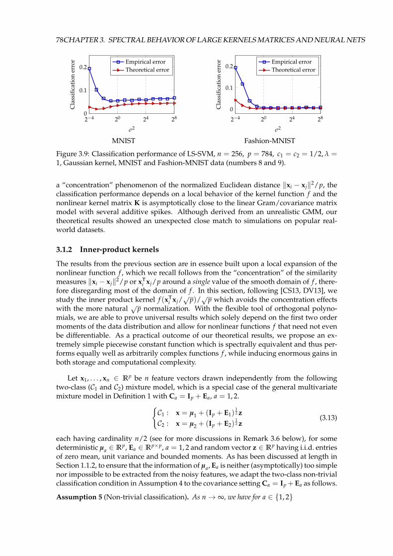
78CHAPTER 3. SPECTRAL BEHAVIOR OF LARGE KERNELS MATRICES AND NEURAL NETS
2−4 20 24 280
0.1
0.2
σ2
Cla
ssifi
cati
oner
ror Empirical error
Theoretical error
MNIST
2−4 20 24 28
0
0.1
0.2
σ2
Cla
ssifi
cati
oner
ror Empirical error
Theoretical error
Fashion-MNIST
Figure 3.9: Classification performance of LS-SVM, n = 256, p = 784, c1 = c2 = 1/2, λ =1, Gaussian kernel, MNIST and Fashion-MNIST data (numbers 8 and 9).
a “concentration” phenomenon of the normalized Euclidean distance ‖xi − xj‖2/p, theclassification performance depends on a local behavior of the kernel function f and thenonlinear kernel matrix K is asymptotically close to the linear Gram/covariance matrixmodel with several additive spikes. Although derived from an unrealistic GMM, ourtheoretical results showed an unexpected close match to simulations on popular real-world datasets.
3.1.2 Inner-product kernels
The results from the previous section are in essence built upon a local expansion of thenonlinear function f , which we recall follows from the “concentration” of the similaritymeasures ‖xi − xj‖2/p or xTi xj/p around a single value of the smooth domain of f , there-fore disregarding most of the domain of f . In this section, following [CS13, DV13], westudy the inner product kernel f (xTi xj/
√p)/√
p which avoids the concentration effectswith the more natural
√p normalization. With the flexible tool of orthogonal polyno-
mials, we are able to prove universal results which solely depend on the first two ordermoments of the data distribution and allow for nonlinear functions f that need not evenbe differentiable. As a practical outcome of our theoretical results, we propose an ex-tremely simple piecewise constant function which is spectrally equivalent and thus per-forms equally well as arbitrarily complex functions f , while inducing enormous gains inboth storage and computational complexity.
Let x1, . . . , xn ∈ Rp be n feature vectors drawn independently from the followingtwo-class (C1 and C2) mixture model, which is a special case of the general multivariatemixture model in Definition 1 with Ca = Ip + Ea, a = 1, 2.
C1 : x = µ1 + (Ip + E1)12 z
C2 : x = µ2 + (Ip + E2)12 z
(3.13)
each having cardinality n/2 (see for more discussions in Remark 3.6 below), for somedeterministic µa ∈ Rp, Ea ∈ Rp×p, a = 1, 2 and random vector z ∈ Rp having i.i.d. entriesof zero mean, unit variance and bounded moments. As has been discussed at length inSection 1.1.2, to ensure that the information of µa, Ea is neither (asymptotically) too simplenor impossible to be extracted from the noisy features, we adapt the two-class non-trivialclassification condition in Assumption 4 to the covariance setting Ca = Ip +Ea as follows.
Assumption 5 (Non-trivial classification). As n→ ∞, we have for a ∈ 1, 2

3.1. RANDOM KERNEL MATRICES 79
1. p/n = c→ c ∈ (0, ∞),
2. ‖µa‖ = O(1), ‖Ea‖ = O(p−1/4), | tr(Ea)| = O(√
p) and ‖Ea‖2F = O(
√p).
Remark 3.5 (On the advantage of proper scaling). It is worth noting that, compared to As-sumption 4 where ‖C1 − C2‖2
F = O(p), here with Assumption 5 the mixture separation isperformed with a higher precision with ‖E1 − E2‖2
F = O(√
p). In this respect, the “properlyscaled” inner-product kernels investigated here is more powerful than the “improperly scaled”ones of form f (xTi xi/p), in separating the covariance “shapes” of Gaussian mixtures.
Following [EK10a, CS13] we consider the following random inner-product kernel ma-trix
K =
δi 6=j f (xTi xj/√
p)/√
pn
i,j=1(3.14)
for f : R 7→ R satisfying Assumption 3. As in [EK10a, CS13], the diagonal elementsf (xTi xi/
√p) have been discarded. Indeed, under Assumption 7, xTi xi/
√p = O(
√p)
which is an “improper scaling” for the evaluation by f (unlike xTi xj/√
p which properlyscales as O(1) for all i 6= j).
In the absence of discriminative information (null model), i.e., if µa = 0 and Ea = 0for a = 1, 2, we write K = KN with
[KN ]ij = δi 6=j f (zTi zj/√
p)/√
p. (3.15)
Letting ξp ≡ zTi zj/√
p, by the central limit theorem, ξpd−→N (0, 1) as p → ∞. As such,
the [KN ]ij, 1 ≤ i 6= j ≤ n, asymptotically behave like a family of dependent standardGaussian variables to which f is applied. In order to analyze the joint behavior of thisfamily, we exploit some useful concepts of the theory of orthogonal polynomials and,in particular, of the class of Hermite polynomials defined with respect to the standardGaussian distribution [AS65, AAR00].
For a real probability measure µ, we denote the set of orthogonal polynomials withrespect to the scalar product 〈 f , g〉 =
∫f gdµ as Pl(x), l = 0, 1, . . ., obtained from the
Gram-Schmidt procedure on the monomials 1, x, x2, . . . such that P0(x) = 1, Pl is ofdegree l and 〈Pl1 , Pl2〉 = δl1−l2 . By the Riesz-Fischer theorem [Rud64, Theorem 11.43], forany function f ∈ L2(µ), the set of squared integrable functions with respect to 〈·, ·〉, onecan formally expand f as
f (x) ∼∞
∑l=0
al Pl(x), al =∫
Rf (x)Pl(x)dµ(x) (3.16)
where “ f ∼ ∑∞l=0 Pl” indicates that ‖ f −∑N
l=0 Pl‖ → 0 as N → ∞ (and ‖ f ‖2 = 〈 f , f 〉).To investigate the asymptotic behavior of K and KN as n, p → ∞, we position our-
selves, as [CS13, DV13] under Assumption 3, which roughly says that the polynomialapproximation of the kernel function f is accurate, for p large, when we truncate theabove expansion at a large but finite degree L.
The limiting parameters a0, a1, a2 and ν appearing in Assumption 3 are simply (gen-eralized) moments of the standard Gaussian measure involving f . Precisely,
a0 = E[ f (ξ)], a1 = E[ξ f (ξ)],√
2a2 = E[(ξ2− 1) f (ξ)] = E[ξ2 f (ξ)], ν = Var[ f (ξ)] ≥ a21 + a2
2
for ξ ∼ N (0, 1). These parameters are of crucial significance in determining the eigen-spectrum behavior of K. Note that a0 will not affect the classification performance, asdescribed below.

80CHAPTER 3. SPECTRAL BEHAVIOR OF LARGE KERNELS MATRICES AND NEURAL NETS
Remark 3.6 (On a0). In the present case of balanced mixtures (equal cardinalities for C1 and C2),a0 contributes to the polynomial expansion of KN (and K) as a non-informative perturbation of theform a0(1n1Tn − In)/
√p. Since 1n is orthogonal to the “class-information vector” [1n/2,−1n/2],
its presence does not impact the classification performance. If mixtures are unbalanced, the vector1n may tend to “pull” eigenvectors aligned to [1n1 ,−1n2 ], with ni the cardinality in Ci, so awayfrom purely noisy eigenvectors and thereby impacting the classification performance. See [CBG16]for similar considerations.
It was shown in [CS13, DV13] that, for independent zi’s with independent entries, theempirical spectral measure (see Definition 5) of the null model KN has an asymptoticallydeterministic behavior as n, p → ∞ with p/n → c ∈ (0, ∞), which depends on thenonlinear f solely via the two parameters (a1, ν), as recalled below.
Theorem 3.3 (Theorem 3.4 in [CS13], Theorem 3 in [DV13]). Under some regularity con-dition for the kernel function f (see Assumption 3 below), the empirical spectral measure of Kconverges weakly and almost surely, as n, p → ∞ with p/n → c ∈ (0, ∞), to a probabil-ity measure µ. The latter is uniquely defined through its Stieltjes transform m : C+ → C+,z 7→
∫(t− z)−1µ(dt) (see also Definition 6 in Section 2.2), given as the unique solution in C+
of the (cubic) equation3
− 1m(z)
= z +a2
1m(z)c + a1m(z)
+ν− a2
1c
m(z)
with a1 = E[ξ f (ξ)] and ν = Var[ f (ξ)] ≥ a21 for standard Gaussian ξ ∼ N (0, 1).
Moreover, Theorem 3.3 is “universal” with respect to the law of the (independent)entries of zi. While universality is classical in random matrix results, with mostly first andsecond order statistics involved, the present universality result is much less obvious sincei) the nonlinear application f (xTi xj/
√p) depends in an intricate manner on all moments
of xTi xj and ii) the entries of KN are strongly dependent. In essence, universality stillholds here because the convergence speed to Gaussian of xTi xj/
√p is sufficiently fast to
compensate the residual impact of higher order moments in the spectrum of KN .
Remark 3.7 (Non-informative spikes). Despite its “universality”, Theorem 3.3 only charac-terizes the limiting spectral measure µ of the kernel matrix K, and thus allows for a “limited”number of isolated eigenvalues to escape from the support of µ. Indeed, as discussed at the end ofSection 2.3, depending on the value of p/n, it was shown in [KC17, FM19] that, for continuouslydifferentiable kernel function f , if a2 6= 0, then K has at most two spikes outside supp(µ), whilefor a2 = 0 all eigenvalues of K lie in supp(µ) almost surely.
As an illustration, Figure 3.10a compares the empirical spectral measure of KN to thelimiting measure obtained from Theorem 3.3.
From a technical viewpoint, our objective here is to go beyond the null model de-scribed in Theorem 3.3 by providing a tractable random matrix equivalent K for the kernelmatrix K, in the sense that ‖K− K‖ → 0 almost surely in operator norm, as n, p → ∞.This convergence allows one to identify the eigenvalues and isolated eigenvectors (thatcan be used for spectral clustering purpose) of K by means of those of K via, for instanceLemma 2.10. More importantly, while not visible from the expression of K, the impact of
3C+ ≡ z ∈ C, =[z] > 0. We also recall that, for m(z) the Stieltjes transform of a measure µ, µ canbe obtained from m(z) via µ([a, b]) = limε↓0
1π
∫ ba =[m(x + ıε)]dx for all a < b continuity points of µ. See
Section 2.1.2 for more details.

3.1. RANDOM KERNEL MATRICES 81
0 5 100 5 10(a) Eigenvalues of KN
0 5 100 5 10(b) Eigenvalues of K
−5
0
5 ·10−2
−5
0
5 ·10−2
(c) Top eigenvectors of KN (top) and K (bot-tom)
Figure 3.10: Eigenvalue distribution and top eigenvector of KN and K, together withthe limiting spectral measure from Theorem 3.3 (in red); f (x) = sign(x), Gaussian zi,n = 2 048, p = 512, µ1 = −[3/2; 0p−1] = −µ2 and E1 = E2 = 0. X = [x1, . . . , xn] ∈ Rp×n
with x1, . . . , xn/2 ∈ C1 and xn/2+1, . . . , xn ∈ C2.
the mixture model (µ1, µ2, E1, E2) on K is readily accessed from K and easily related to theHermite coefficients ( a1, a2, ν ) of f . This allows us to further investigate how the choiceof f impacts the asymptotic feasibility and efficiency of spectral clustering from the topeigenvectors of K.
Main results. The main idea for the asymptotic analysis of K comes in two steps: first,by an expansion of xTi xj as a function of zi, zj and the statistical mixture model param-eters µ, E, we decompose xTi xj (under Assumption 7) into successive orders of magni-tudes with respect to p; this, as we will show, further allows for a Taylor expansionof f (xTi xj/
√p) for at least twice differentiable functions f around its dominant term
f (zTi zj/√
p). Then, we rely on the orthogonal polynomial approach of [CS13] to “lin-earize” the resulting matrix terms f (xTi xj/
√p), f ′(xTi xj/
√p) and f ′′(xTi xj/
√p)
(all terms corresponding to higher order derivatives asymptotically vanish) and use As-sumption 3 to extend the result to arbitrary square-summable f .
Our main conclusion is that K asymptotically behaves like a matrix K following aso-called “spiked random matrix model” in the sense that K = KN + KI is the sumof the full-rank “noise” matrix KN having compact limiting spectrum and a low-rank“information” matrix KI [BAP05, BGN11].
We first show that K can be asymptotically approximated as KN + KI with KN de-fined in (3.15) and KI an additional (so far full-rank) term containing the statistical infor-mation of the mixture model.
As announced, we start by decomposing xTi xj into a sequence of terms of successiveorders of magnitude using Assumption 7 and xi = µa + (Ip + Ea)
12 zi, xj = µb + (Ip +
Eb)12 zj for xi ∈ Ca and xj ∈ Cb. We have precisely, for i 6= j,
xTi xj√p
=µT
a µb√p
+1√
p(µT
a (Ip + Eb)12 zj + µT
b (Ip + Ea)12 zi) +
1√
pzTi (Ip + Ea)
12 (Ip + Eb)
12 zj
=zTi zj√
p︸ ︷︷ ︸O(1)
+zTi (Ea + Eb)zj
2√
p︸ ︷︷ ︸≡Aij=O(p−1/4)
+µT
a µb + µTa zj + µT
b zi√p
−zTi (Ea − Eb)
2zj
8√
p︸ ︷︷ ︸≡Bij=O(p−1/2)
+o(p−1/2) (3.17)

82CHAPTER 3. SPECTRAL BEHAVIOR OF LARGE KERNELS MATRICES AND NEURAL NETS
where in particular we performed a Taylor expansion of (Ip +Ea)12 (since ‖Ea‖ = O(p−
14 ))
around Ip, and used the fact that with high probability zTi Eazj = O(p1/4) and zTi (Ea −Eb)
2zj = O(1).
As a consequence of this expansion, for at least twice differentiable f ∈ L2(µp), wehave
Kij =f (xTi xj/
√p)
√p
=f (zTi zj/
√p)
√p
+f ′(zTi zj/
√p)
√p
(Aij +Bij)+f ′′(zTi zj/
√p)
2√
pA2
ij + o(p−1)
where o(p−1) is understood with high probability and uniformly over i, j ∈ 1, . . . , n.Recall that, this entry-wise expansion up to order o(p−1) is sufficient since, matrix-wise, ifAij = o(p−1) uniformly on i, j, from ‖A‖ ≤ p‖A‖∞ = p maxi,j |Aij|, we have ‖A‖ = o(1)as n, p→ ∞.
In the particular case where f is a monomial of degree k ≥ 2, this implies the follow-ing result.
Proposition 3.1 (Monomial f ). Under Assumptions 3 and 5, let f (x) = xk, k ≥ 2. Then, asn, p→ ∞,
‖K− (KN + KI)‖ → 0 (3.18)
almost surely, with KN defined in (3.15) and
KI =k√
p(ZTZ/
√p)(k−1) (A + B) +
k(k− 1)2√
p(ZTZ/
√p)(k−2) (A)2 (3.19)
for Z = [z1, . . . , zn] ∈ Rp×n and A, B ∈ Rn×n defined in (3.17) with Aii = Bii = 0. Here X Ydenotes the Hadamard product between X, Y and Xk the k-th Hadamard power, i.e., [Xk]ij =(Xij)
k.
Since f ∈ L2(µ) can be decomposed into its Hermite polynomials, Proposition 3.1along with Theorem 3.3 allows for an asymptotic quantification of K. However, the ex-pression of KI in (3.19) does not so far allow for a thorough understanding of the spec-trum of K, due to 2) the delicate Hadamard products between purely random (ZTZ) andinformative matrices (A, B) and ii) the fact that KI is full rank (so that the resulting spec-tral properties of KN + KI remains intractable). We next show that, as n, p → ∞, KIadmits a tractable low-rank approximation KI , thereby leading to a spiked-model ap-proximation for K.
Let us consider KI defined in (3.19), the (i, j) entry of which can be written as the sumof terms containing µa, µb (treated separately) and random variables of the type
φ =C√
p(xTy/
√p)α(xTFy)β
for independent random vectors x, y ∈ Rp with i.i.d. zero mean, unit variance and finitemoments (uniformly on p) entries, deterministic F ∈ Rp×p, C ∈ R, α ∈N and β ∈ 1, 2.
For Gaussian x, y, the expectation of φ can be explicitly computed via an integral trick[Wil97, LLC18]. For more generic x, y with i.i.d. bounded moment entries, a combinato-rial argument controls the higher order moments of the expansion which asymptoticallyresult in (matrix-wise) vanishing terms. See Sections A.1.4 in the appendix. This leads tothe following result.

3.1. RANDOM KERNEL MATRICES 83
Proposition 3.2 (Low rank asymptotics of KI). Under Assumptions 3 and 5, for f (x) = xk,k ≥ 2,
‖KI − KI‖ → 0
almost surely as n, p→ ∞, for KI defined in (3.19) and
KI =
k!!p (JMTMJT + JMTZ + ZTMJT), for k odd
k(k−1)!!2p J (T + S) JT, for k even
(3.20)
where4
M = [µ1, µ2] ∈ Rp×2, T = tr(Ea + Eb)/√
p2a,b=1, S = tr(EaEb)/
√p2
a,b=1 ∈ R2×2
and J = [j1, j2] ∈ Rn×2 with ja ∈ Rn the canonical vector of class Ca, i.e., [ja]i = δxi∈Ca .
We refer the readers to Section A.1.4 of the Appendix for a detailed exposition of theproof.
Proposition 3.2 states that KI is asymptotically equivalent to KI that is of rank at mosttwo.5 Note that the eigenvectors of KI are linear combinations of the vectors j1, j2 andthus provide the data classes.
From the expression of KI , quite surprisingly, it appears that for f (x) = xk, depend-ing on whether k is odd or even, either only the information in means (M) or only incovariance (T and S) can be (asymptotically) preserved.
By merely combining the results of Propositions 3.1–3.2, the latter can be easily ex-tended to polynomial f . Then, by considering f (x) = Pκ(x), the Hermite polynomial ofdegree κ, it can be shown that, quite surprisingly, one has KI = 0 if κ > 2. As such,using the Hermite polynomial expansion P0, P1, . . . of an arbitrary f ∈ L2(µ) satisfyingAssumption 3 leads to a very simple expression of our main result.
Theorem 3.4 (Spiked-model approximation of K). For an arbitrary f ∈ L2(µ) with f ∼∑∞
l=0 al Pl(x), under Assumptions3 and 5,
‖K− K‖ → 0, K = KN + KI
with KN defined in (3.15) and
KI =a1
p(JMTMJT + JMTZ + ZTMJT) +
a2
pJ(T + S)JT. (3.21)
Proof. The proof of Theorem 3.4 follows from the fact that the individual coefficientsof the Hermite polynomials Pκ(x) = ∑κ
l=0 cκ,lxl satisfy the following recurrent relation[AS65]
cκ+1,l =
−κcκ−1,l l = 0;cκ,l−1 − κcκ−1,l l ≥ 1;
(3.22)
4For mental reminder, M stands for means, T accounts for the difference in traces of covariance matricesand S for the “shapes” of the covariances.
5Note that, as defined, KI has non-zero diagonal elements, while [KI ]ii = 0. This is not contradictory asthe diagonal matrix diag(KI) has vanishing norm and can thus be added without altering the approximation‖KI − KI‖ → 0; it however appears convenient as it ensures that KI is low rank (while without its diagonal,KI is full rank).

84CHAPTER 3. SPECTRAL BEHAVIOR OF LARGE KERNELS MATRICES AND NEURAL NETS
with c0,0 = 1, c1,0 = 0 and c1,1 = 1. As a consequence, by indexing the informative matrixin Proposition 3.2 of the monomial f (x) = xl as KI,l , we have for odd κ ≥ 3,
KI =κ
∑l=1,3,...
cκ,lKI,l =κ
∑l=1,3,...
cκ,l l!!(JMTMJT + JMTZ + ZTMJT)/p− diag(·) = 0
with [X − diag(·)]ij = Xijδi 6=j. This follows from the fact that, for κ ≥ 3, we have both∑κ
l=1,3,... cκ,l l!! = 0 and ∑κ+1l=0,2,... cκ+1,l(l + 1)!! = 0. The latter is proved by induction on κ:
first, for κ = 3, we have c3,1 + 3c3,3 = c4,0 + 3c4,2 + 15c4,4 = 0; then, assuming κ odd, wehave ∑κ
l=1,3,... cκ,l l!! = ∑κ+1l=0,2,... cκ+1,l(l + 1)!! = 0 so that, together with (3.22)
κ+2
∑l=1,3,...
cκ+2,l l!! =κ+2
∑l=1,...
(cκ+1,l−1− (κ+ 1)cκ,l)l!! =κ+2
∑l=1,...
cκ+1,l−1l!! =κ+1
∑l=0,2,...
cκ+1,l(l + 1)!! = 0
as well asκ+3
∑l=0,2,...
cκ+3,l(l + 1)!! = −(κ + 2)cκ+1,0 +κ+3
∑l=2,4,...
(cκ+2,l−1 − (κ + 2)cκ+1,l)(l + 1)!! = 0
where we used cκ,l = 0 for l ≥ κ + 1. Similar arguments hold for the case of κ even, whichconcludes the proof.
−1 0 1 1.5−1 0 1 1.5(a) N : eigs of K for P1
−1 0 1 1.5−1 0 1 1.5(b) N : eigs of K for P1
−2 −1 0 1 2−2 −1 0 1 2−2 −1 0 1 2(c) N : eigs of K for P2
−2 −1 0 1 2−2 −1 0 1 2−2 −1 0 1 2(d) N : eigs of K for P2
−1 0 1 1.5−1 0 1 1.5(e) Stud: eigs of K for P1
−1 0 1 1.5−1 0 1 1.5(f) Stud: eigs of K for P1
−2 −1 0 1 2
(g) Stud: eigs of K for P3
−2 −1 0 1 2
(h) Stud: eigs of K for P3
Figure 3.11: Eigenvalue distributions of K and K from Theorem 3.4 (blue) and L fromTheorem 3.3 (red), for zi with Gaussian (top) or Student-t with degree of freedom 7 (bot-tom) entries; functions f (x) = P1(x) = x, f (x) = P2(x) = (x2 − 1)
√2, f (x) = P3(x) =
(x3 − 3x)/√
6; n = 2 048, p = 8 192, µ1 = −[2; 0p−1] = −µ2 and E1 = −10Ip/√
p = −E2.
Figure 3.11 compares the spectra of K and K for random vectors with independentGaussian or Student-t entries, for the first three (normalized) Hermite polynomials P1(x),P2(x) and P3(x). These numerical evidences validate Theorem 3.4: only for P1(x) andP2(x) is an isolated eigenvalue observed. Besides, as shown in the bottom display of Fig-ure 3.10c, the corresponding eigenvector is, as expected, a noisy version of linear combi-nations of j1, j2.

3.1. RANDOM KERNEL MATRICES 85
Table 3.2: Storage size and top eigenvectorrunning time of K for piecewise constantand cubic f , in the setting of Figure 3.11and 3.13.
f Size (Mb) Running time (s)Piecewise 4.15 0.2390Cubic 16.75 0.4244
Figure 3.12: Piecewise constant (green)versus cubic (BLUE) function with equal(a1, a2, ν).
Remark 3.8 (Even and odd f ). While rank(KI) ≤ 4 (as the sum of two rank-two terms), inFigure 3.11 no more than two isolated eigenvalues are observed (for f = P1 only one on theright side, for f = P2 one on each side). This follows from a2 = 0 when f = P1 and a1 = 0 forf = P2. More generally, for f odd ( f (−x) = − f (x) ), a2 = 0 and the statistical informationon covariances (through E) asymptotically vanishes in K; for f even ( f (−x) = f (x)), a1 = 0and the information about the means µ1, µ2 vanishes. Thus, only f neither odd nor even canpreserve both first and second order discriminating statistics (e.g., the popular ReLU functionf (x) = max(0, x)). This was previously remarked in [LC18a] based on a local expansion ofsmooth f in a similar setting.
Practical consequences. As a direct consequence of Theorem 3.4, the performance ofspectral clustering for large dimensional mixture models of the type (3.13) only dependson the three parameters of the nonlinear function f : a1 = E[ξ f (ξ)], a2 = E[ξ2 f (ξ)]/
√2
and ν = E[ f 2(ξ)]. The parameters a1, ν determine the limiting spectral measure L of K(since K and KN asymptotically differ by a rank-4 matrix, they share the same limitingspectral measure) while a2, a2 determine the low rank structure within KI .
As an immediate consequence, arbitrary (square-summable) kernel functions f (witha0 = 0) are asymptotically equivalent to the simple cubic function f (x) = c3x3 + c2x2 +c1x − c2 having the same Hermite polynomial coefficients a1, a2, ν, due to the followingrelation
a1 = 3c3 + c1, a2 =√
2c2, ν = (3c3 + c1)2 + 6c2
3 + 2c22.
The idea here to design a prototypical family F of functions f having i) universalproperties with respect to (a1, a2, ν), i.e., for each (a1, a2, ν) there exists f ∈ F with theseHermite coefficients and ii) having numerically advantageous properties. Thus, any ar-bitrary kernel function f can be mapped, through (a1, a2, ν), to a function in F with goodnumerical properties.
One such prototypical family F can be the set of f , parametrized by (t, s−, s+), anddefined as
f (x) =
−rt x ≤
√2s−
0√
2s− < x ≤√
2s+t x >
√2s+
with
a1 = t√
2π(e−s2
+ + re−s2−)
a2 = t√2π(s+e−s2
+ + rs−e−s2−)
ν = t2
2 (1− erf(s+)) (1 + r)
(3.23)
where r ≡ 1−erf(s+)1+erf(s−)
. Figure 3.12 displays f given in (3.23) together with the cubic functionc3x3 + c2(x2 − 1) + c1x sharing the same Hermite coefficients (a1, a2, ν).
The class of equivalence of kernel functions induced by this mapping is quite unlikethat raised in [EK10b] or [CBG16] in the “improper” scaling f (xTi xj/p) regime. While in

86CHAPTER 3. SPECTRAL BEHAVIOR OF LARGE KERNELS MATRICES AND NEURAL NETS
the latter, functions f (x) of the same class of equivalence are those having common f ′(0)and f ′′(0) values, in the present case, these functions may have no similar local behavior(as shown in the example of Figure 3.12).
For the piecewise constant function defined in (3.23) and the associated cubic func-tion having the same (a1, a2, ν), a close match is observed for both eigenvalues and topeigenvectors of K in Figure 3.13, with gains in both storage size and computational timedisplayed in Table 3.2.
−0.5 0 0.5 1−0.5 0 0.5 1(a) Piecewise constant
−0.5 0 0.5 1−0.5 0 0.5 1(b) Cubic polynomial
−5
0
·10−2
(c) Cubic (blue) versus piecewise (green) func-tion
Figure 3.13: Eigenvalue distribution and top eigenvectors of K for the piecewise constantfunction (in green) and the associated cubic function (in blue) with the same (a1, a2, ν),performed on Bernoulli distribution with zero mean and unit variance, in the setting ofFigure 3.11.
Conclusion. In this last section, we evaluated the eigenspectrum of the “properly-scaled”inner-product kernel matrix K = f (XTX/
√p)/√
p. Built upon the flexible tool of orthog-onal polynomials, we showed that the spectrum of K depends on the kernel function fvia three “global” key parameters (a1, a2, ν), and this holds true for a large range of non-linear functions f , including even some non-smooth functions. In this vein, all kernelfunctions under study are equivalent, in an eigenspectrum sense, to a cubic function, aswell as to a piecewise function that takes only three values, as long as they share the same(a1, a2, ν).
To close this section on random kernel matrices, according to the discussion in Re-mark 3.5, it is of future interest to extend the current analyses on f (XTX/
√p)/√
p tocover data with an arbitrary covariance matrix C (that is not limited to C = I + E with‖E‖ = o(1)). However, this is technically more involved, since it breaks most of theorthogonality properties of the orthogonal polynomial approach of the proofs, but is aneeded extension of the result.
It would also be of interest to properly scale not only the inner-product kernels, butalso other popular choice of kernels such as the shift-invariant kernels studied in Sec-tion 3.1.1. From this perspective, the kernel matrices of the type f (‖xi‖2/p− 2xTi xi/
√p+
‖xj‖2/p) could be a good starting point.
3.2 Random Neural Networks
As discussed in Section 1.2.2, the fundamental connection between random kernel matri-ces and random weights NN models can be built upon random feature maps. In this sub-

3.2. RANDOM NEURAL NETWORKS 87
section, we demonstrate how random kernel matrices appear in the performance analysisof single-hidden-layer random NN models, and how this analysis allows us to evaluatethe impact on performance of the activation function.
3.2.1 Large neural networks with random weights
X ∈ Rp×n
σσσσσ
Σ ≡ σ(WX) ∈ RN×nβTΣ
W ∈ RN×pβ ∈ RN×d
Figure 3.14: Illustration of a single-hidden-layer random NN
In this section, we consider the single-hidden-layer random NN model (or, randomfeature-based kernel ridge regression) illustrated above (same as Figure 1.3).
For a data matrix X =[x1, . . . , xn
]∈ Rp×n with associated targets Y =
[y1, . . . , yn
]∈
Rd×n, we denote Σ ∈ RN×n the output of the middle layer comprising in total N neuronsof X by premultiplying some (random) weight matrix W ∈ RN×p with i.i.d. standardGaussian entries and then passing through some nonlinear activation function σ : R 7→ R
to obtain Σ ≡ σ(WX) ∈ RN×n. In particular, we focus on the case where the secondlayer weight matrix β ∈ RN×d is designed to minimize the regularized MSE: L(β) =1n ∑n
i=1 ‖yi− βTσ(Wxi)‖2 + λ‖β‖2F on the given deterministic training set (X, Y), for some
regularization factor λ > 0. This givens the following explicit form (as in (1.18)) for β:
β ≡ 1n
Σ
(1n
ΣTΣ + λIn
)−1
YT. (3.24)
We are interested in the asymptotic behavior of the training and test MSE of the net-work (as in (1.19)) defined by
Etrain =1n
n
∑i=1‖yi − βTσ(Wxi)‖2 =
1n‖Y− βTΣ‖2
F, Etest =1n‖Y− βTΣ‖2
F (3.25)
on a (deterministic) test set (X, Y) of size n, i.e., X ∈ Rp×n, Y ∈ Rd×n, where we similarlydenote Σ ≡ σ(WX) ∈ RN×n.
Let us start with the training error Etrain. Note that, by defining the resolvent (seeDefinition 4) of the Gram matrix 1
n ΣTΣ as
Q(z = −λ) = Q ≡(
1n
ΣTΣ + λIn
)−1
∈ Rn×n
the training MSE of interest can be rewritten as
Etrain =1n‖Y− βTΣ‖2
F =λ2
ntr(YQ2YT) = −λ2
n∂ tr(YQYT)
∂λ(3.26)
and is therefore wished to establish an asymptotically deterministic behavior as the sumof aTQb for deterministic vector a, b ∈ Rn of bounded Euclidean norm (with the nor-malization n−1). if we could find a deterministic equivalent (see Definition 7) for Q.
To properly state our main results, the following assumptions are needed.

88CHAPTER 3. SPECTRAL BEHAVIOR OF LARGE KERNELS MATRICES AND NEURAL NETS
Assumption 6 (Lipschitz σ). The function σ is Lipschitz continuous with parameter indepen-dent of n, p.
Assumption 7 (Growth rate in random NN). As n→ ∞,
1. p/n→ c1 ∈ (0, ∞) and N/n→ c2 ∈ (0, ∞);
2. X has a bounded operator norm, i.e., ‖X‖ = O(1);
3. Y has bounded entries, i.e., ‖Y‖∞ = O(1).
Note that, for the nonlinear Gram matrix 1n ΣTΣ, with σ(t) = t one merely gets the
sample covariance/Gram matrix 1n XTWTWX, the spectrum of which is known to have
an asymptotic deterministic behavior (recall Section 2.2.3) with ‖X‖ = O(1). Intuitivelyspeaking, Assumption 6 ensures that the nonlinear activation σ “varies” in a “controlled”manner.
Also, by demanding Y to have bounded entries as n, p, N → ∞, we indeed ask therows of Y, together with the n−1/2 normalization, to have bounded Euclidean norm, soas to apply our deterministic equivalent approach.
Under Assumptions 6 and 7, with a we are now ready to prove the concentration ofthe resolvent Q (in the sense that ‖Q−EW[Q]‖ → 0) as n, p, N → ∞, and consequentlywe can provide an exact characterization of the training and test MSE in (1.19).
Main results. Before going into our main results, let us first re-introduce the following“equivalent” kernel matrix (as in (1.20))
K = Ew[σ(XTw)σ(wTX)] (3.27)
for w ∼ N (0, Ip). Again, the appearance of kernel matrix K here is rather natural sincethe Gram matrix 1
n ΣTΣ at the heart of our analysis is indeed an approximation of K underthe random feature framework, for instance with ψw(x) = σ(wTx) in (1.15).
To show the concentration of the resolvent Q (as well as the eigenspectrum) of aGram/sample covariance-like random matrix ZTZ, a concentration of quadratic formsbased on the row vectors of Z is necessary. For instance, recall from Section 2.2.2 that,to show the (almost sure) convergence of 1
n tr A( 1
n ZTZ− zIn)−1
for Z ∈ Rp×n havingi.i.d. standard Gaussian entries, we exploited the concentration of quadratic form result1n zTi Azi − 1
n tr A a.s.−→0 in Lemma 2.11, to bound the difference between( 1
n ZTZ− zIn)−1
and( 1
n ZTZ− 1n zizTi − zIn
)−1, for z ∈ Rn the i-th row of Z so that zi ∼ N (0, In). In gen-
eral, such concentration of quadratic form results are obtained by exploiting the indepen-dence (or linear dependence) in the vector entries (e.g., zi ∼ N (0, In) in the Marcenko-Pastur case in Section 2.2.2). For the nonlinear model under consideration
1n
ΣTΣ =1n
σ(WX)Tσ(WX)
the desired independence unfortunately does not hold, since the entries of the vectorσ(XTw) are in general not independent. To overcome this technical difficulty, we resortto a concentration of measure approach, as advocated in [Kar09]. The following lemmaprovides this concentration result.
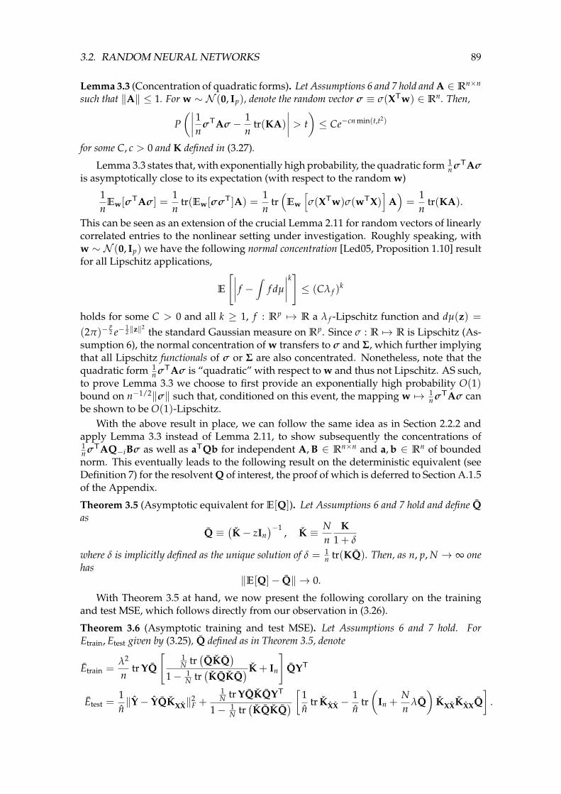
3.2. RANDOM NEURAL NETWORKS 89
Lemma 3.3 (Concentration of quadratic forms). Let Assumptions 6 and 7 hold and A ∈ Rn×n
such that ‖A‖ ≤ 1. For w ∼ N (0, Ip), denote the random vector σ ≡ σ(XTw) ∈ Rn. Then,
P(∣∣∣∣ 1n σTAσ − 1
ntr(KA)
∣∣∣∣ > t)≤ Ce−cn min(t,t2)
for some C, c > 0 and K defined in (3.27).
Lemma 3.3 states that, with exponentially high probability, the quadratic form 1n σTAσ
is asymptotically close to its expectation (with respect to the random w)
1n
Ew[σTAσ] =
1n
tr(Ew[σσT]A) =1n
tr(
Ew
[σ(XTw)σ(wTX)
]A)=
1n
tr(KA).
This can be seen as an extension of the crucial Lemma 2.11 for random vectors of linearlycorrelated entries to the nonlinear setting under investigation. Roughly speaking, withw ∼ N (0, Ip) we have the following normal concentration [Led05, Proposition 1.10] resultfor all Lipschitz applications,
E
[∣∣∣∣ f − ∫ f dµ
∣∣∣∣k]≤ (Cλ f )
k
holds for some C > 0 and all k ≥ 1, f : Rp 7→ R a λ f -Lipschitz function and dµ(z) =
(2π)−p2 e−
12 ‖z‖2
the standard Gaussian measure on Rp. Since σ : R 7→ R is Lipschitz (As-sumption 6), the normal concentration of w transfers to σ and Σ, which further implyingthat all Lipschitz functionals of σ or Σ are also concentrated. Nonetheless, note that thequadratic form 1
n σTAσ is “quadratic” with respect to w and thus not Lipschitz. AS such,to prove Lemma 3.3 we choose to first provide an exponentially high probability O(1)bound on n−1/2‖σ‖ such that, conditioned on this event, the mapping w 7→ 1
n σTAσ canbe shown to be O(1)-Lipschitz.
With the above result in place, we can follow the same idea as in Section 2.2.2 andapply Lemma 3.3 instead of Lemma 2.11, to show subsequently the concentrations of1n σTAQ−iBσ as well as aTQb for independent A, B ∈ Rn×n and a, b ∈ Rn of boundednorm. This eventually leads to the following result on the deterministic equivalent (seeDefinition 7) for the resolvent Q of interest, the proof of which is deferred to Section A.1.5of the Appendix.
Theorem 3.5 (Asymptotic equivalent for E[Q]). Let Assumptions 6 and 7 hold and define Qas
Q ≡(K− zIn
)−1 , K ≡ Nn
K1 + δ
where δ is implicitly defined as the unique solution of δ = 1n tr(KQ). Then, as n, p, N → ∞ one
has‖E[Q]− Q‖ → 0.
With Theorem 3.5 at hand, we now present the following corollary on the trainingand test MSE, which follows directly from our observation in (3.26).
Theorem 3.6 (Asymptotic training and test MSE). Let Assumptions 6 and 7 hold. ForEtrain, Etest given by (3.25), Q defined as in Theorem 3.5, denote
Etrain =λ2
ntr YQ
[1N tr
(QKQ
)1− 1
N tr(KQKQ
) K + In
]QYT
Etest =1n‖Y− YQKXX‖
2F +
1N tr YQKQYT
1− 1N tr
(KQKQ
) [ 1n
tr KXX −1n
tr(
In +Nn
λQ)
KXXKXXQ]
.

90CHAPTER 3. SPECTRAL BEHAVIOR OF LARGE KERNELS MATRICES AND NEURAL NETS
Then, as n, p, N → ∞Etrain − Etrain → 0, Etest − Etest → 0
almost surely, with
KAB ≡ Ew
[σ(wTA)Tσ(wTB)
], KAB ≡
Nn
KAB
1 + δ, K ≡ KXX, K ≡ KXX.
We also mention here that, while the above finding on the (asymptotic) training MSEalways holds true under Assumptions 6 and 7, the test MSE presented is only a conjec-ture which not be proved under a general situation, for example with only ‖X‖ = O(1)and ‖Y‖∞ = O(1). Under some statistical assumptions for (X, Y) (e.g., GMM as in Defini-tion 1) the conjecture is valid [LC18b]. Further empirical evidences on real-world datasetsalso show an extremely close match. This leads to the fundamental question on the min-imal (statistical) assumption on the data to establish an asymptotically deterministic be-havior for neural networks performances. A first promising answer is given in [LC18b]by assuming the data to be concentrated random vectors, e.g., Lipschitz maps of standardGaussian random vector or of vectors with i.i.d. entries. Intuitively speaking, this meansthat the high dimensional data are random, but in a “concentrated” manner such that, in-stead of “spreading” all over their large ambient space, the data live within a rather lowdimensional layer. As a consequence, each scalar observation of these data, even withcomplicated function such as regressor or classifier, tends to have an almost determinis-tic and predictable behavior, that depends only on the first several order of statistics ofthe data.
Practical consequences. Theorem 3.6 allows to assess the training and test performanceof the network, via the equivalent kernel matrix K (and K) built from the (determin-istic) data. It thus remains to compute this kernel matrix K, which is given under theform of an expectation/integral with respect to the standard Gaussian distribution (ofdimension p). For most commonly used nonlinear activations σ(·), the generic formK(a, b) = Ew[σ(wTa)σ(wTb)] can be computed explicitly via an integral trick [Wil97],for arbitrary vector a, b ∈ Rp. We list the results for commonly used functions in Ta-ble 3.3, with computational details provided in Section A.1.6 of the Appendix.
Table 3.3: K(a, b) for different σ(·), ∠(a, b) ≡ aTb‖a‖‖b‖ .
σ(t) K(a, b)t aTbmax(t, 0) 1
2π‖a‖‖b‖(∠(a, b) arccos (−∠(a, b)) +
√1−∠(a, b)2
)|t| 2
π‖a‖‖b‖(∠(a, b) arcsin (∠(a, b)) +
√1−∠(a, b)2
)1t>0
12 −
12π arccos (∠(a, b))
sign(t) 2π arcsin (∠(a, b))
ς2t2 + ς1t + ς0 ς22
(2(aTb
)2+ ‖a‖2‖b‖2
)+ ς2
1aTb + ς2ς0(‖a‖2 + ‖b‖2)+ ς2
0
cos(t) exp(− 1
2
(‖a‖2 + ‖b‖2)) cosh(aTb)
sin(t) exp(− 1
2
(‖a‖2 + ‖b‖2)) sinh(aTb)
erf(t) 2π arcsin
(2aTb√
(1+2‖a‖2)(1+2‖b‖2)
)exp(−t2/2) 1√
(1+‖a‖2)(1+‖b‖2)−(aTb)2

3.2. RANDOM NEURAL NETWORKS 91
To corroborate the findings in Theorem 3.6 we consider the task of classifying theMNIST database [LBBH98] with a single-hidden-layer random weight neural networkcomposed of N = 512 hidden-units. Similar to Section 3.1.1 we represent each image asa p = 784-size vector; 1 024 images of sevens and 1 024 images of nines were extractedfrom the database and were evenly split in 512 training and test images, respectively, sothat n = n = 1 024. The database images were jointly centered and scaled so to fall closeto the setting of Assumption 7 on X and X. The columns of the output values Y and Ywere taken as unidimensional (d = 1) with Yi, Yi ∈ −1, 1 depending on the imageclass. Figure 3.15 displays the simulated (averaged over 100 realizations of W) versustheoretical values of Etrain and Etest for three choices of Lipschitz continuous functionsσ(·), as a function of the regularization factor λ. We observe an almost perfect matchbetween the simulations and our theoretical results from Theorem 3.6 for not so largen, p, N.
10−4 10−3 10−2 10−1 100 101 102
10−1
100
σ(t) = max(t, 0)
σ(t) = erf(t)
σ(t) = t
λ
MSE
Etrain (Theory)Etest (Theory)
Etrain (Simulation)Etest (Simulation)
Figure 3.15: Performance of the network for Lipschitz σ, as a function of λ, for MNISTdata (number 7 and 9), N = 512, n = n = 1024, p = 784.
Conclusion. In this section, we characterized the resolvent Q of 1n ΣTΣ with Σ = σ(WX)
the output of a random NN with input X and showed it establishes an asymptoticallydeterministic behavior for Lipschitz activations σ(·). As a direct consequence, we gavethe training and test MSE of the random NN model in Figure 1.3 that depends on the dataand the activation function σ(·) via the key “equivalent” kernel matrix K ≡ Ew[σ(XTw)σ(wTX)].For most commonly used σ, the expression of K is given in Table 3.3.
Nonetheless, the expressions of K in Table 3.3 are still in very barely interpretable andprovide little understanding of the role played by the nonlinear activations. For instance,we are not able to say which σ(·) should be used for a given task. To further exploitthe interplay between the data and the activation function, we next investigate in thefollowing section the eigenspectrum of K by (additionally) considering a GMM for theinput data.

92CHAPTER 3. SPECTRAL BEHAVIOR OF LARGE KERNELS MATRICES AND NEURAL NETS
3.2.2 Random feature maps and the equivalent kernels
We saw in the previous section that the single-layer random NN performance depends onthe deterministic data X and the nonlinear activation σ(·) via the following “equivalent”kernel matrix (as in (1.20))
K ≡ Ew[σ(XTw)σ(wTX)]
the expression of which is explicitly given in Table 3.3 for most commonly used σ withw ∼ N (0, Ip). In this section we develop a deeper understanding of, the eigenspectrumof this kernel matrix K, for structural statistical models for X. In particular, we focuson the interplay between σ and the data statistics µ, C of X under a GMM as detailed inDefinition 1.
In the context of random feature maps, 1n ΣTΣ is indeed the Gram matrix of the ran-
dom features σ(Wxi), that approximates an underlying kernel matrix as discussed at theend of Section 1.2.1. From Theorem 3.5, we know that the resolvent of 1
n ΣTΣ and thus itslimiting spectral measure, if exists, are both closely related to K. In this vein, the kernelmatrix K above is again at the heart of all random feature-based spectral algorithms.
Consider x1, . . . , xn ∈ Rp independent data vectors, each belonging to one of K dis-tribution classes C1, . . . , CK. Class Ca has cardinality na, for all a ∈ 1, . . . , K. The datavector xi that belongs to Ca is assumed to be drawn from the following GMM
xi =1√
pµa + ωi
with ωi ∼ N (0, Ca/p) for some mean µa ∈ Rp and covariance Ca ∈ Rp×p that satisfythe non-trivial classification in Assumption 2. Note that we normalize the data by 1/
√p,
together with Assumption 2 to ensure ‖xi‖ = O(1) with high probability, which is inconsistent with Assumption 7 in the presented random NN model.
Taking a = xi and b = xj, we see that the expressions of K in Table 3.3 are indeednonlinear functions of the “concentrated” measures of the data, e.g., ‖xi‖ or xTi xj, asinvestigated in Section 3.1.1 under the binary setting K = 2. Therefore, the spectralanalysis of K for GMM under Assumption 2 follows exactly the same line of argumentsas in [CBG16] and discussed at length in Section 3.1.1, that we briefly recall next.
From a random feature map standpoint, the Gram matrix 1n ΣTΣ describes the corre-
lation of data in the feature space. It is thus natural to recenter 1n ΣTΣ, hence K, by pre- and
post-multiplying with the projection matrix P ≡ In − 1n 1n1Tn . In the case of K, we get
Kc ≡ PKP.
This centering operation technically eliminates, from a technical standpoint, the non-informative isolated eigenvalues that may go to infinity as n, p→ ∞, with correspondingnon-informative eigen-direction 1n.
Main results. Let us now introduce the key steps of our present analysis. Under As-sumption 2, observe that for xi ∈ Ca and xj ∈ Cb, i 6= j,
xTi xj = ωTi ωj︸ ︷︷ ︸
O(p−1/2)
+ µTa µb/p + µT
a ωj/√
p + µTb ωi/
√p︸ ︷︷ ︸
O(p−1)

3.2. RANDOM NEURAL NETWORKS 93
which allows one to perform a Taylor expansion around 0 as p, T → ∞, to give a rea-sonable approximation of nonlinear functions of xTi xj, such as those appearing in Kij (seeagain Table 3.3). For i = j, one has instead
‖xi‖2 = ‖ωi‖2︸ ︷︷ ︸O(1)
+ ‖µa‖2/p + 2µT
a ωi/√
p︸ ︷︷ ︸O(p−1)
.
From Eωi [‖ωi‖2] = tr(Ca)/p it is convenient to further write
‖ωi‖2 = tr(Ca)/p +(‖ωi‖2 − tr(Ca)/p
)where tr(Ca)/p = O(1) and ‖ωi‖2 − tr(Ca)/p = O(n−1/2). By definition6 τ ≡ tr(C)/pthat is assumed to converge in (0, ∞) as in the two-class case in Assumption 4. Exploitingagain Assumption 2, one results in,
‖xi‖2 = τ︸︷︷︸O(1)
+ tr(Ca)/p + ‖ωi‖2 − tr(Ca)/p︸ ︷︷ ︸O(p−1/2)
+ ‖µa‖2/p + 2µT
a ωi/√
p︸ ︷︷ ︸O(p−1)
which allows for a Taylor expansion of nonlinear functions of ‖xi‖2 around τ, as done forxTi xj.
From Table 3.3, it appears that, for every listed σ(·), K(xi, xj) is a smooth function ofxTi xj and ‖xi‖, ‖xj‖, despite their possible discontinuities (for example, the ReLU functionand σ(t) = |t|). The above results therefore allow for an entry-wise Taylor expansion ofthe matrix K in the large n, p limit.
A critical aspect of the analysis where random matrix theory comes into play nowconsists in developing K as a sum of matrices arising from the Taylor expansion andignoring terms that give rise to a vanishing operator norm, so as to find an asymptoticequivalent matrix K such that ‖K− K‖ → 0 as n, p → ∞, as described in detail below.This analysis provides a simplified asymptotically equivalent expression for K with allnonlinearities removed.
To present our main theoretical result, we define, similarly to Section 3.1.1 and 3.1.2the following notations for random elements
Ω ≡[ω1, . . . , ωn
]∈ Rp×n, φ ≡
‖ωi‖2 −E
[‖ωi‖2]n
i=1 ∈ Rn
as well as for deterministic elements7,
M ≡[µ1, . . . , µK
]∈ Rp×K, J ≡
[j1, . . . , jK
]∈ Rn×K
t ≡
1√
ptr Ca
K
a=1∈ RK, S ≡
1p
tr(CaCb)
K
a,b=1∈ RK×K
where ja ∈ Rn denotes, as usual, the canonical vector of class Ca such that (ja)i = δxi∈Ca .
Theorem 3.7 (Asymptotic equivalent of Kc). Let Assumption 2 hold and Kc be defined asKc ≡ PKP for K given in (1.20). Then, as n→ ∞, for all σ(·) given in Table 3.3,
‖Kc − Kc‖ → 0
6Note that the notation τ defined here differs from that in Section 1.1.2 and 3.1.1 by a factor 2.7Similarly to Section 3.1.2, M stands for means, t accounts for (difference in) traces while S for the “shapes”
of covariances. Note in particular that the definition of S is different from that in Section 3.1.2, since only thespecial case Ca = Ip + Ea is considered in Section 3.1.2.

94CHAPTER 3. SPECTRAL BEHAVIOR OF LARGE KERNELS MATRICES AND NEURAL NETS
almost surely, with Kc = PKP and
K ≡ d1
(Ω + M
JT√
p
)T (Ω + M
JT√
p
)+ d2UBUT + d0In ≡ KN + KI + d0In
where we recall that P ≡ In − 1n 1n1Tn and
U ≡[
J√p , φ
], B ≡
[ttT + 2S t
tT 1
], KN ≡ d1ΩTΩ + d2φφT
KI ≡d1
p(JMTMJT +
√pΩTMJT +
√pJMTΩ) +
d2
p
(J(ttT + 2S)JT +
√pφtTJT +
√pJtφT
)with the coefficients d0, d1, d2 given in Table 3.4.
Table 3.4: Coefficients di in Kc for different σ(·).
σ(t) d0 d1 d2
t 0 1 0
ReLU(t) ≡ max(t, 0)( 1
4 −1
2π
)τ 1
41
8πτ
|t|(1− 2
π
)τ 0 1
2πτ
ς+ max(t, 0) + ς−max(−t, 0)≡ LReLU(t)
π−24π (ς+ + ς−)2τ 1
4 (ς+ − ς−)2 18τπ (ς+ + ς−)2
1t>014 −
12π
12πτ 0
sign(t) 1− 2π
2πτ 0
ς2t2 + ς1t + ς0 2τ2ς22 ς2
1 ς22
cos(t) 12 +
e−2τ
2 − e−τ 0 e−τ
4
sin(t) 12 −
e−2τ
2 − τe−τ e−τ 0
erf(t) 2π
(arccos
( 2τ2τ+1
)− 2τ
2τ+1
) 4π
12τ+1 0
exp(−t2/2) 1√2τ+1− 1
τ+1 0 14(τ+1)3
Theorem 3.7 tells us as a corollary (from for example Lemma 2.10) that the maxi-mal difference between the eigenvalues of Kc and Kc vanishes asymptotically as n, p →∞. Similarly the distance between the “isolated eigenvectors” also vanishes. This is oftremendous importance as the determination of the leading eigenvalues and eigenvectorsof Kc (that contain crucial information for clustering, for example) can be studied fromthe equivalent problem performed on Kc and becomes mathematically more tractable.
It is also of interest to remark from Theorem 3.7 that, albeit derived from differentdata models and kernel types, Theorem 3.7 provides the same intuition as Theorem 3.4:the first order information (M) always goes with one coefficient (d1 and a1, respectively),while the second order information (t, S or T, S, respectively) is always multiplied byanother coefficient (d2 and a2, respectively).
To make this clear, the major differences between these two results are summarizedas follows:
1. Theorem 3.4 characterizes the spectrum of the “properly scaled” inner-product ker-nel matrix model f (xTi xj/
√p), with zero on its diagonal, regardless of the underly-
ing distribution; it holds for any square-summable kernel function f (that satisfies

3.2. RANDOM NEURAL NETWORKS 95
Assumption 3); the coefficients a1, a2 and ν are known to be the (generalized) mo-ments of f (with respect to standard Gaussian measure). Nonetheless, due to thelack of more advanced technical tools, only the special case Ca = Ip + Ea is coveredin Theorem 3.4.
2. On the other hand, Theorem 3.7 treats the kernel matrices arising from randomfeature maps (or random NNs), in the Gaussian case (i.e., for GMM data); thesekernels are “improperly scaled” (as those studied in Section 3.1.1) with the formf (xTi xj/p) in Table 3.3, and the analysis is based on a local expansion of f , whichimperatively demands f to be locally (at least three-times) differentiable near 0 andτ. Also, Theorem 3.7 holds only for the nonlinear activation listed in Table 3.3for which we are capable of explicitly computing the expression of K. However,Theorem 3.7 holds for arbitrary covariance Ca.
Practical consequences. On closer inspection of Theorem 3.7, the matrix K is expressedas the sum of three terms, weighted respectively by the three coefficients d0, d1 and d2,that depend on the nonlinear function σ(·) via Table 3.4. Note that the statistical structureof the data xin
i=1 (namely the means in M and the covariances in t and S) is perturbedby random fluctuations (Ω and φ). In this perspective, we see that d1 and d2 (asymp-totically) control the “expression” of the first (M) and second order (t and S) statisticalinformation in K, respectively. In particular, there exists a balance between the meansand covariances, that provides some instructions in the appropriate choice of the nonlin-earity. From Table 3.4, the functions σ(·) can be divided into the following three groups:
• mean-oriented, where d1 6= 0 while d2 = 0: this is the case of the functions t, 1t>0,sign(t), sin(t) and erf(t), which asymptotically track only the difference in means(i.e., t and S disappear from the expression of Kc);
• covariance-oriented, where d1 = 0 while d2 6= 0: this concerns the functions |t|, cos(t)and exp(−t2/2), which asymptotically track only the difference in covariances;
• balanced, where both d1, d2 6= 0: here for the ReLU function max(t, 0) and thequadratic function ς2t2 + ς1t + ς0.
To corroborate the above classification of different nonlinearity, we perform kernelspectral clustering in Figure 3.16 on four classes of Gaussian data: N (µ1, C1), N (µ1, C2),N (µ2, C1) and N (µ2, C2) with the LReLU function that takes different values for ς+ andς−. For a = 1, 2, µa =
[0a−1; 5; 0p−a
]and Ca = (1 + 15(a − 1)/
√p)Ip. By choosing
ς+ = −ς− = 1 (equivalent to σ(t) = |t|) and ς+ = ς− = 1 (equivalent to the linearmap σ(t) = t), with the leading two eigenvectors we always recover two classes insteadof four, as each setting of parameters only allows for a part of the statistical informationof the data to be used for clustering. However, by taking ς+ = 1, ς− = 0 (the ReLUfunction) we distinguish all four classes in the leading two eigenvectors, to which thek-means method can then be applied for final classification, as shown in Figure 3.17.
We complete this section by showing that our theoretical results in Theorem 3.7, de-rived from GMMs, show an unexpected close match in practice when applied to real-world datasets. We consider two different types of classification tasks: one on the MNIST[LBBH98] database (number 6 and 8), and the other on epileptic EEG time series data[ALM+01] (set B and E). These two datasets are typical examples of means-dominant

96CHAPTER 3. SPECTRAL BEHAVIOR OF LARGE KERNELS MATRICES AND NEURAL NETS
C1 C2 C3 C4
(a) σ(t) = |t|: eigenvector 1
C1 C2 C3 C4
(b) σ(t) = |t|: eigenvector 2
C1 C2 C3 C4
(c) σ(t) = t: eigenvector 1
C1 C2 C3 C4
(d) σ(t) = t: eigenvector 2
Figure 3.16: Leading two eigenvectors of Kc for the LReLU function with ς+ = −ς− = 1(top) and ς+ = ς− = 1 (bottom), performed on four classes Gaussian mixture data withp = 512, n = 256, ca = 1/4 and ja = [0na−1 ; 1na ; 0n−na ], for a = 1, 2, 3, 4. Expectationestimated by averaging over 500 realizations of W.
Table 3.5: Empirical estimation of (normalized) differences in means and covariances ofthe MNIST (Figure 3.18) and epileptic EEG (Figure 3.19) datasets.
‖MTM‖ ‖ttT + 2S‖MNIST data 172.4 86.0EEG data 1.2 182.7
(handwritten digits recognition) and covariances-dominant (EEG times series classifi-cation) tasks. This is numerically confirmed in Table 3.5 (see also Table 3.1 from Sec-tion 3.1.1).
We perform random feature-based spectral clustering on data matrices that consistof n = 32, 64 and 128 randomly selected vectorized images of size p = 784 from theMNIST dataset. Means and covariances are empirically obtained from the full set of11 769 MNIST images (5 918 images of number 6 and 5 851 of number 8). Comparingthe matrix Kc built from the data and the theoretically equivalent Kc obtained as if thedata were Gaussian with the (empirically) computed means and covariances, we observean extremely close fit in the behavior of the eigenvalues and the leading eigenvector inFigure 3.18. The k-means method is then applied to the leading two eigenvectors of theGram matrix 1
n ΣTΣ that consists of N = 32 random features to perform unsupervisedclassification, with resulting accuracies (averaged over 50 runs) reported in Table 3.6.As seen from Table 3.5, the mean-oriented σ(t) functions are expected to outperform thecovariance-oriented functions in this task, which is consistent with the results in Table 3.6.

3.2. RANDOM NEURAL NETWORKS 97
Eigenvector 1
C1 C2 C3 C4
Eigenvector 2
C1 C2 C3 C4
Eigenvector 1
Eige
nvec
tor
2
Figure 3.17: Leading two eigenvectors of Kc (top) for the LReLU function with ς+ = 1,ς− = 0 (equivalent to ReLU(t)) and two dimensional representation of these eigenvectors(bottom), in the same setting as in Figure 3.16.
Table 3.6: Classification accuracies for random feature-based spectral clustering with dif-ferent σ(t) on the MNIST dataset.
σ(t) n = 32 n = 64 n = 128
mean-oriented
t 85.31% 88.94% 87.30%1t>0 86.00% 82.94% 85.56%
sign(t) 81.94% 83.34% 85.22%sin(t) 85.31% 87.81% 87.50%erf(t) 86.50% 87.28% 86.59%
cov-oriented
|t| 62.81% 60.41% 57.81%cos(t) 62.50% 59.56% 57.72%
exp(−t2/2) 64.00% 60.44% 58.67%balanced ReLU(t) 82.87% 85.72% 82.27%
The epileptic EEG dataset8, developed by the University of Bonn, Germany, is de-scribed in [ALM+01]. The dataset consists of five subsets (denoted A-E), each containing100 single-channel EEG segments of 23.6-sec duration. Sets A and B were collected fromsurface EEG recordings of five healthy volunteers, while sets C, D and E were collectedfrom the EEG records of the pre-surgical diagnosis of five epileptic patients. Here we per-form random feature-based spectral clustering on n = 32, 64 and 128 randomly pickedEEG segments of length p = 100 from the dataset. Means and covariances are empir-
8http://www.meb.unibonn.de/epileptologie/science/physik/eegdata.html.

98CHAPTER 3. SPECTRAL BEHAVIOR OF LARGE KERNELS MATRICES AND NEURAL NETS
1 2 3 4 5 60
0.5
1
1.5Eigenvalues of Kc
Eigenvalues of Kc
1 2 3 4 5 60
0.5
1
1.5Eigenvalues of Kc
Eigenvalues of Kc
1 2 3 4 5 60
0.5
1
1.5Eigenvalues of Kc
Eigenvalues of Kc
Leading eigenvector for MNIST dataSimulation: mean/std for MNIST dataTheory: mean/std for Gaussian data
C1 C2
Figure 3.18: Eigenvalue distribution of Kc and Kc for the MNIST data (left) and leadingeigenvector of Kc for the MNIST and Gaussian mixture data (right) with a width of ±1standard deviations (generated from 500 trials). With the ReLU function, p = 784, n =128 and c1 = c2 = 1/2, j1 = [1n1 ; 0n2 ] and j2 = [0n1 ; 1n2 ].
ically estimated from the full set (4 097 segments of set B and 4 097 segments of set E).Similar behavior of eigenpairs as for Gaussian mixture models is once more observedin Figure 3.19. After k-means classification on the leading two eigenvectors of the (cen-tered) Gram matrix composed of N = 32 random features, the accuracies (averaged over50 runs) are reported in Table 3.7.
As opposed to the MNIST image recognition task, from Table 3.7 it is easy to checkthat the covariance-oriented functions (i.e., σ(t) = |t|, cos(t) and exp(−t2/2)) far outper-form any other with almost perfect classification accuracies. It is particularly interestingto note that the popular ReLU function is suboptimal in both tasks, but never performsvery badly, thereby offering a good risk-performance tradeoff.
2 4 6 80
0.1
0.2
0.3Eigenvalues of Kc
Eigenvalues of Kc
Leading eigenvector for EEG dataSimulation: mean/std for EEG dataTheory: mean/std for Gaussian data
C1 C2
Figure 3.19: Eigenvalue distribution of Kc and Kc for the epileptic EEG data (left) andleading eigenvector of Kc for the EEG and Gaussian mixture data (right) with a width of±1 standard deviations (generated from 500 trials). With the ReLU function, p = 100, n =128 and c1 = c2 = 1/2, j1 = [1n1 ; 0n2 ] and j2 = [0n1 ; 1n2 ].
Conclusion. In this section, by leveraging the randomness of the data, we dived deepinto the comprehension of the equivalent kernel matrix K = Ew[σ(XTw)σ(wX)] that ap-pears in the random NN context (in Section 3.2.1) as well as in random feature-basedtechniques. The same technical approach as in Section 3.1.1 was applied to handle the

3.3. EMPIRICAL RISK MINIMIZATION OF CONVEX LOSS 99
Table 3.7: Classification accuracies for random feature-based spectral clustering with dif-ferent σ(t) on the epileptic EEG dataset.
σ(t) n = 32 n = 64 n = 128
mean-oriented
t 71.81% 70.31% 69.58%1t>0 65.19% 65.87% 63.47%
sign(t) 67.13% 64.63% 63.03%sin(t) 71.94% 70.34% 68.22%erf(t) 69.44% 70.59% 67.70%
cov-oriented
|t| 99.69% 99.69% 99.50%cos(t) 99.00% 99.38% 99.36%
exp(−t2/2) 99.81% 99.81% 99.77%balanced ReLU(t) 84.50% 87.91% 90.97%
nonlinearity arising from the activation function σ(·). Despite the difference in datamodels and technical approaches, we reached a similar conclusion on the classification ofdifferent σ as in Section 3.1.2, i.e., two key parameters (d1, d2) control separately the sta-tistical information in means and covariance. Experiments on typical real-world datasetswere performed to validate our theoretical arguments.
3.3 Empirical Risk Minimization of Convex Loss
In Section 3.1 and 3.2 we discussed both large random kernel matrices (and kernel ridgeregression build on top of it) as well as random NN/feature-based models that are closelyconnected to one another. However, all aforementioned objects of interest are in thesemachine learning methods assume closed forms, as they come in essence from the min-imization of (regularized) square losses. More generally, almost all machine learning al-gorithms are given in form of (solutions of) optimization problems, with most of them ex-pressed only in an implicit manner. An important example is the popular logistic regres-sion, where one aims to find an optimal decision vector β ∈ Rp by minimizing the logisticloss 1
n ∑ni=1 log(1 + e−yi β
Txi) over the training set (xi, yi)ni=1 with labels yi ∈ −1,+1.
Different from the linear regression solution that arises from the minimization of squareloss, the logistic regression solution β takes an implicit form and it is less direct to un-derstand how β depends on the data X so as to investigate its statistical behavior. Thetechnical challenge from implicit optimization problems appears not only in the analysisof logistic regression, but also in many other machine learning algorithms in daily use.
In this regard, it is of crucial importance to adapt the proposed random matrix-basedanalysis framework to assess the performance of optimization-based learning methods,we evaluate here the classifier obtained by minimizing an arbitrary convex and differen-tiable loss, with a major emphasis on the “leave-one-out” technical approach to “decou-ple” the learning system that contains complicated dependences.
In this section, we consider the following (regularized) empirical risk minimizationproblem (as in (1.22))
minβ∈Rp
1n
n
∑i=1
L(yiβTxi) +
λ
2‖β‖2 (3.28)

100CHAPTER 3. SPECTRAL BEHAVIOR OF LARGE KERNELS MATRICES AND NEURAL NETS
under a binary symmetric GMM for the input data, i.e.,C1 : xi = −µ + C
12 zi, yi = −1
C2 : xi = +µ + C12 zi, yi = +1
(3.29)
each with a class prior of 1/2, for z ∼ N (0, Ip), µ ∈ Rp and positive definite C ∈ Rp×p.Let us first consider the case where λ > 0 and the existence of the minimizer β is
guaranteed. Similar to the non-trivial classification condition in Assumption 2, we shallposition ourselves under the following assumption.
Assumption 8 (Non-trivial classification). As n → ∞, we have p/n → c ∈ (0, ∞), ‖µ‖ =O(1) and max‖C‖, ‖C−1‖ = O(1) with respect to p.
Note that the GMM in (3.29) satisfies the logistic regression model in the sense thatthe conditional class probability is given by
P(yi = 1 | xi ∈ C2) =1
1 + exp(−2µTC−1xi)≡ σ(βT
∗ xi)
with σ(t) = (1 + e−t)−1 the logistic sigmoid function and the optimal Bayes solution β∗ =2C−1µ. With the GMM in (3.29) and labels yi ∈ −1,+1, it is convenient to denote theshortcut xi ≡ yixi so that
xi ∼ N (µ, C)
regardless of the class to which xi belongs.
To investigate the asymptotic performance of the empirical risk-based classifier in(3.28), it is of crucial importance to understand the statistical properties of β that mini-mizes (3.28). The main technical difficulty of this analysis lies in the fact that β, as thesolution of a convex optimization problem, does not have an explicit form. Nonethe-less, by canceling the loss function derivative with respect to β we obtain the followingimplicit relation
λβ =1n
n
∑i=1−L′(βTxi)xi (3.30)
where we assume the loss function L is convex and at least three-times differentiable. Inthis section, in addition to RMT techniques, in order to handle the implicit nature of β, wemainly focus on the additional “leave-one-out” tool to handle the complex dependencesin the optimization problem.
Main results. From (3.30), β can be seen as a linear combination of all xi’s, weightedby the coefficient −L′(βTxi). The idea is to understand how xi (and its statistical prop-erties) affects the corresponding coefficient −L′(βTxi). However, as a solution of (3.30),β depends on all xi’s in an intricate manner. We handle this correlation by establishinga “leave-one-out” version of β, denoted β−i, that is asymptotically close to β and inde-pendent of xi, by solving (3.28) for all data xj different from xi, i.e., for j = 1, . . . , i− 1, i +1, . . . , n.
In details, since by definition λβ−i = − 1n ∑j 6=i L′(βT
−ixj)xj, the difference λ(β− β−i)is given by
λ(β− β−i) =1n ∑
j 6=i
(L′(βT
−ixj)− L′(βTxj))
xj −1n
L′(βTxi)xi (3.31)

3.3. EMPIRICAL RISK MINIMIZATION OF CONVEX LOSS 101
Intuitively speaking, under Assumption 8, the difference ‖β− β−i‖ should be small,in the sense that it goes to 0 as n, p→ ∞. As such, by a Taylor expansion of L′(x) aroundx = βT
−ixj, j 6= i, we obtain
L′(βTxj) = L′(βT−ixj) + L′′(βTxj)(β− β−i)
Txj + O(‖β− β−i‖2).
This approximation, together with (3.31), leads to the following relation on β− β−i
λ(β− β−i) ' −1n ∑
j 6=iL′′(βT
−ixj)xjxTj (β− β−i)−1n
L′(βTxi)xi
or in matrix form (1n
X−iD−iXT−i + λIp
)(β− β−i) ' −
1n
L′(βTxi)xi
with D−i ≡ diagL′′(βT−ixj)n
j 6=i ∈ R(n−1)×(n−1) and X−i ∈ Rp×(n−1) the data matrixwithout xi.
Note here that by convexity of L, L′′(t) ≥ 0 for all t, so that with λ > 0, the matrix( 1n X−iDXT
−i + λIp)
is invertible and we get
β− β−i ' −1n
L′(βTxi)
(1n
X−iD−iXT−i + λIp
)−1
xi
so that its projection on xi gives
(β− β−i)Txi ' −
1n
L′(βTxi)xTi
(1n
X−iD−iXT−i + λIp
)−1
xi.
Note that( 1
n X−iDXT−i + λIp
)−1is of bounded operator norm and independent of xi.
Following the idea of Lemma 2.11 we deduce the following approximation.
Lemma 3.4 (Asymptotic approximation of quadratic forms). Let Assumption 8 holds. Thenas n, p→ ∞,
1n
xTi
(1n
X−iD−iXT−i + λIp
)−1
xi − κa.s.−→0
where κ is the unique positive solution of κ = 1n tr(QC) with
Q ≡(
E
[L′′(βTx)
1 + κL′′(βTx)
]C + λIp
)−1
.
As a consequence of Lemma 3.4, one has immediately
(β− β−i)Txi ' −L′(βTxi)κ
and thereforeβTxi = βT
−ixi + (β− β−i)Txi ' βT
−ixi − L′(βTxi)κ
where we observe the quantity βTxi on both sides, which is given by the explicit equation
βTxi ' proxκL(βT−ixi)

102CHAPTER 3. SPECTRAL BEHAVIOR OF LARGE KERNELS MATRICES AND NEURAL NETS
with proxκL(t) the proximal operator [BC11] defined as the unique solution of the followingminimization problem
minx∈R
κL(x) +12(βT−ixi − x)2.
The uniqueness of the minimization problem above is guaranteed by the convexity ofthe loss L. Moreover, the proximal operator can be defined for all lower semi-continuousconvex functions, and thus covers non-smooth loss L(t) such as the hinge losses L(t) =max(1 − t, 0). In this vein, our results are envisioned to extend to non-smooth losses,for which more refinements (to replace the gradient with the subgradient in the sense ofClarke [Cla90] and to rework on Lemma 3.4) are needed.
Since β−i is independent of xi, we have βT−ixi ∼ N (m, σ2) in the large p limit for some
unknown deterministic m and σ2, as summarized in the following lemma.
Lemma 3.5. Under Assumption 8, there exist two positive constants m, σ2 such that, as n, p→∞,
βT−ixi − r d−→0, r ∼ N (m, σ2)
and
L′(βTxi)− f (r) d−→0, f (r) ≡ L′(proxκL(r)) =r− proxκL(r)
κ
with the proximal operator proxκL(r) defined as the unique solution of the following minimiza-tion problem
minx∈R
κL(x) +12(x− r)2
for some κ > 0 determined by the fixed point equation in Lemma 3.4.
With Lemma 3.5, to characterize the stochastic behavior of βT−ixi and βTxi (and sub-
sequently β), it remains to determine the unknown constants m and σ2. This can be doneby taking the expectation on both sides of (3.30) as
λE[β] =1n
n
∑i=1−E
[f (βT−ixi)xi
]which helps connect the statistics of β to m and σ2. Nonetheless, the right-hand-sideexpectation in the above equation is non-trivial, due to the dependence between the ran-dom vector xi and its projection xTi β−i onto the independent β−i.
Fortunately, in the case of Gaussian xi ∼ N (µ, C), this dependence can be separatedand treated explicitly. By writing xi = µ +
√pωi with ωi ∼ N (0, C/p) we can decom-
pose ωi as the following sum
ωi =βT−iωi
βT−iCβ−i
Cβ−i + ω⊥i 'βT−iωi
tr CE[β−iβT−i]
Cβ−i + ω⊥i 'βT−iωi
σ2 Cβ−i + ω⊥i
for σ2 defined in Lemma 3.4 and such that ωTi β−i is independent of ω⊥i , i.e.,
Eωi
[ω⊥i ωT
i β−i
]= Eωi
[(ωi −
βT−iωi
βT−iCβ−i
Cβ−i
)ωT
i β−i
]= 0
and in particular βT−iω
⊥i = 0. As a consequence, (3.30) can be reduced to
λβ ' 1n
n
∑i=1− f (βT
−ixi)
(µ +
√pβT−iωi
σ2 Cβ−i +√
pω⊥i
)
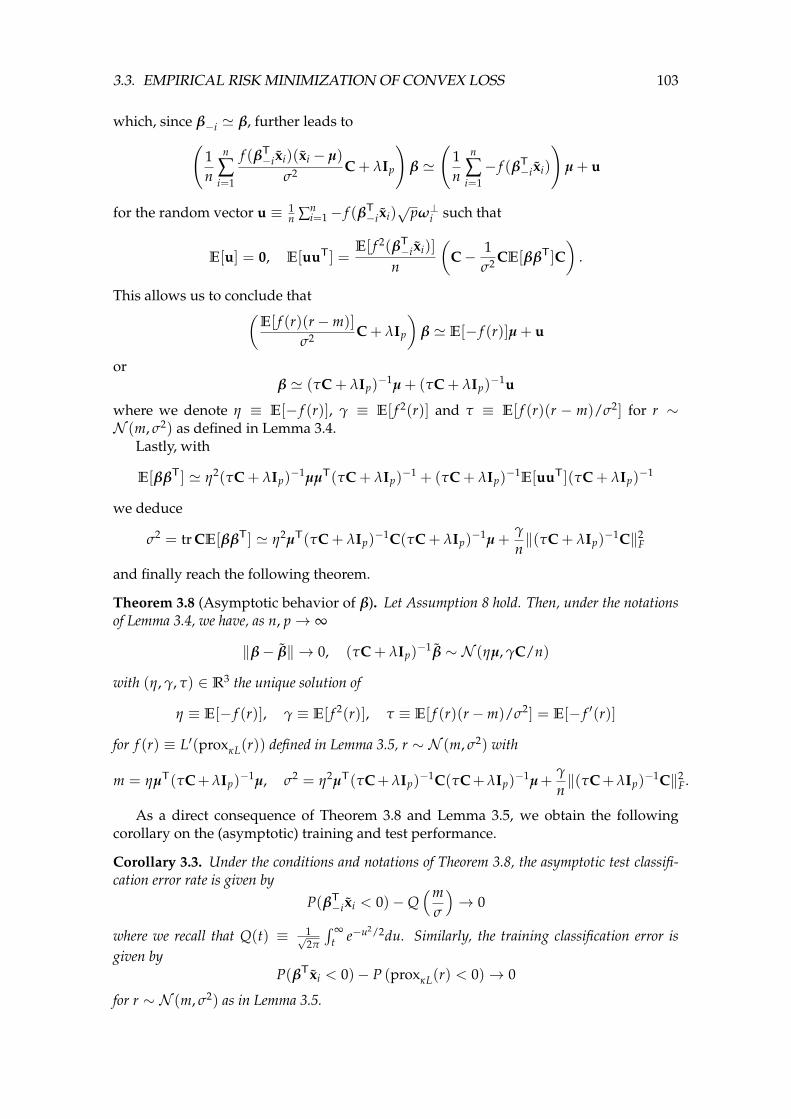
3.3. EMPIRICAL RISK MINIMIZATION OF CONVEX LOSS 103
which, since β−i ' β, further leads to(1n
n
∑i=1
f (βT−ixi)(xi − µ)
σ2 C + λIp
)β '
(1n
n
∑i=1− f (βT
−ixi)
)µ + u
for the random vector u ≡ 1n ∑n
i=1− f (βT−ixi)
√pω⊥i such that
E[u] = 0, E[uuT] =E[ f 2(βT
−ixi)]
n
(C− 1
σ2 CE[ββT]C)
.
This allows us to conclude that(E[ f (r)(r−m)]
σ2 C + λIp
)β ' E[− f (r)]µ + u
orβ ' (τC + λIp)
−1µ + (τC + λIp)−1u
where we denote η ≡ E[− f (r)], γ ≡ E[ f 2(r)] and τ ≡ E[ f (r)(r − m)/σ2] for r ∼N (m, σ2) as defined in Lemma 3.4.
Lastly, with
E[ββT] ' η2(τC + λIp)−1µµT(τC + λIp)
−1 + (τC + λIp)−1E[uuT](τC + λIp)
−1
we deduce
σ2 = tr CE[ββT] ' η2µT(τC + λIp)−1C(τC + λIp)
−1µ +γ
n‖(τC + λIp)
−1C‖2F
and finally reach the following theorem.
Theorem 3.8 (Asymptotic behavior of β). Let Assumption 8 hold. Then, under the notationsof Lemma 3.4, we have, as n, p→ ∞
‖β− β‖ → 0, (τC + λIp)−1β ∼ N (ηµ, γC/n)
with (η, γ, τ) ∈ R3 the unique solution of
η ≡ E[− f (r)], γ ≡ E[ f 2(r)], τ ≡ E[ f (r)(r−m)/σ2] = E[− f ′(r)]
for f (r) ≡ L′(proxκL(r)) defined in Lemma 3.5, r ∼ N (m, σ2) with
m = ηµT(τC+λIp)−1µ, σ2 = η2µT(τC+λIp)
−1C(τC+λIp)−1µ+
γ
n‖(τC+λIp)
−1C‖2F.
As a direct consequence of Theorem 3.8 and Lemma 3.5, we obtain the followingcorollary on the (asymptotic) training and test performance.
Corollary 3.3. Under the conditions and notations of Theorem 3.8, the asymptotic test classifi-cation error rate is given by
P(βT−ixi < 0)−Q
(mσ
)→ 0
where we recall that Q(t) ≡ 1√2π
∫ ∞t e−u2/2du. Similarly, the training classification error is
given byP(βTxi < 0)− P (proxκL(r) < 0)→ 0
for r ∼ N (m, σ2) as in Lemma 3.5.

104CHAPTER 3. SPECTRAL BEHAVIOR OF LARGE KERNELS MATRICES AND NEURAL NETS
0 1 20
0.2
0.4
0.6
0.8
1 Empirical distribution of βT−i xi
Gaussian distribution N (m, σ2)
Figure 3.20: Comparison between the histogram of βT−ixi and the Gaussian distribution
N (m, σ2) defined in Theorem 3.8 with µ = [2, 0p−1], Cp = Ip, for λ = 1, p = 256 andn = 512.
Practical consequences. To validate Theorem 3.8 and Lemma 3.5 for n, p of reasonablesizes, we compare in Figure 3.20 the empirical distribution of βT
−ixi and the Gaussiandistribution N (m, σ2) from the system of fixed point equations in Theorem 3.8. Ourtheoretical results fit the simulation almost perfectly, already for p = 256 and n = 512.
To interpret Theorem 3.8 we first restrict ourselves to the unregularized case whereλ = 0 and assume the minimization problem (3.28) admits a solution β such that ‖β‖ =O(1), at least with high probability. Note that depending on the problem (µ, C and theloss L) and the dimensionality (n, p), such a solution may not exist with λ = 0 (for in-stance as pointed out in [CS18] for the logistic regression L(t) = log(1 + e−t)).
With λ = 0, the notations in Theorem 3.8 are reduced to
β ∼ N(η
τC−1µ,
γ
nτIp
)with m = η
τ µTC−1µ and σ2 = η2
τ2 µTC−1µ + γτ2
pn . Several remarks are in order:
1. E[β] is aligned to the optimal Bayes solution β∗ = 2C−1µ. However, unlike in theregime where n → ∞ and p fixed, β contains an additional zero mean Gaussiannoise of covariance γ
nτ Ip, which results in a larger variability of the soft output βTxthan classical asymptotics predict.
2. The scaling of β depends on the interplay between the data statistics (µ, C), theproblem dimensionality (n, p) and the loss function L. In general, E[β] differs fromthe optimal Bayes solution β∗ by a multiplicative (constant) factor, i.e., E[β] = η
2τ β∗.In Figure 3.21 we examine the empirical mean (so as to estimate the expectation)of β, the rescaled version 2τ
η β and the optimal Bayes solution β∗. We see that byrescaling the obtained β by the factor 2τ/η, one gets (in expectation) the optimalβ∗. Nonetheless, note that for classification applications, one has sign(βTx) =
sign(aβTx) for a > 0, meaning that a positive rescaling of β does not affect theclassification performance.
3. As a consequence of Corollary 3.3, in pursuit of an optimal design of the loss func-tion L, one must find (η, γ, τ) that maximizes the ratio m2/σ2, or equivalently
arg max(η,γ,τ)∈R3
m2
σ2 = arg max(η,γ,τ)∈R3
(µTC−1µ)2
µTC−1µ + γη2
pn= arg max
(η,γ,τ)∈R3
η2
γ

3.3. EMPIRICAL RISK MINIMIZATION OF CONVEX LOSS 105
where we recall η = E[− f (r)] and γ = E[ f 2(r)], so that by Cauchy–Schwarz in-equality
η2 ≤ γ
with equality if and only if f (r) is a constant function. The minimal misclassifica-
tion error rate is therefore given by Q(mσ ) = Q
(µTC−1µ√
µTC−1µ+p/n
)for the model under
consideration. On the other hand, it is of interest to note that, by the law of largenumbers, the empirical average 1
n ∑ni=1−L′(βTxi) converges to its expectation η as
n → ∞, and similarly for γ. As such, one may alternatively wish to maximize thefollowing empirical version
max(η,γ,τ)∈R3
L′(βTX)1n√L′(βTX)L′(XTβ)
where the function L′ is applied entry-wise on the vector βTX ∈ Rn. Under theabove form, note from (3.30) that in the unregularized case with λ = 0 one musthas
XL′(XTβ) = 0
so that by considering a singular value decomposition of X = UΣVT = U[S 0
] [VT1
VT2
]for X ∈ Rp×n with n > p such that S ∈ Rp×p, V1 ∈ Rn×p and V2 ∈ Rn×(n−p), onemust have VT
1 L′(XTβ) = 0, or equivalently, L′(XTβ) lies on the subspace spannedby the columns vectors of V2 such that there exists a ∈ Rn−p for which
L′(XTβ) = V2a.
With the formulation, one aims to find
arg max(η,γ,τ)∈R3
aTVT2 1n
‖a‖
which attains the maximum if and only if a is aligned to VT2 1n a = aVT
2 1n forsome a > 0. This optimality condition is met for instance with the square lossL(t) = (t− 1)2.
Conclusion. In this section, we considered the separation of a symmetric binary GMMwith opposite means±µ and identical covariance C, by minimizing the empirical convexand differentiable risk L on a given training set. In this scenario, the statistical of theresulting classifier β depends on the chosen loss metric via the generalized moment of anonlinear function f (x) ≡ L′(proxκL(x)) with respect to the standard Gaussian measure,in an implicit manner via the proximal operator and the constant κ > 0. As a consequenceof the analysis, we saw that the in the regime n, p → ∞ with p/n → c ∈ (0, ∞), βis the sum of a rescaled of β∗, the optimal Bayes solution, together with an additionalhomogeneous Gaussian noise.

106CHAPTER 3. SPECTRAL BEHAVIOR OF LARGE KERNELS MATRICES AND NEURAL NETS
10 20 30 40 50 60−0.2
−0.1
0
0.1
0.2
Index
β∗β2τη β
Figure 3.21: Comparison of the empirical mean of β (denoted β) the solution of (1.22) forlogistic loss L(t) = log(1 + e−t), the optimal Bayes solution β∗ and the rescaled solution2τη β for (η, τ) derived from Theorem 3.8 with µ = [1p/3,−1p/3, 3
4 1p/3]/√
p, C = 2Ip, forp = 60, n = 300. Empirical means obtained by averaging over 500 realizations.
3.4 Summary of Chapter 3
In this chapter, we focused on the eigenspectrum of large dimensional random kernelmatrices and neural networks. Built upon a simple Gaussian mixture modeling of theinput data, we provided a tractable characterization of the spectral behavior of kernelmatrices and nonlinear Gram matrices, from which we further deduced the (asymptotic)performance of various machine learning methods, as a function of the data statistics,the dimensionality, and the hyperparameters of the algorithm. The presented theoreti-cal findings shed novel light on the understanding, as well as a better designing of theaforementioned machine learning methods.
To further address more involved learning algorithms, for example, those (implic-itly) defined by convex optimization problems (e.g., logistic regression), we resort to a“leave-one-out” approach and assume that the optimality conditions are met. By work-ing on these conditions, we deduced the (asymptotic) performance reached by the opti-mal points of the these optimization problems.
In practice, optimization methods such a gradient descent are regularly used to reachthese optimal points. The solution of the optimization problem, and therefore its per-formance, naturally depends on the optimization method applied. The impact of theoptimization method is more significant in non-convex problems, where depending onthe initialization, totally different solutions can be reached. In the following chapter, wefocus precisely on the gradient descent algorithm and study its behavior in convex andnon-convex machine learning problems.

Chapter 4
Gradient Descent Dynamics inNeural Networks
In Chapter 3 we discussed either kernel-based methods that are of explicit forms (in Sec-tion 3.1.1–3.2.2), or the statistical behavior of the unique minimum from a convex opti-mization problem (in Section 3.3), without considering by which means can we reach thisoptimum. In this chapter, we discuss the possibly most widely used gradient descentmethod, and in particular, the temporal evolution of (the performance of) the learningsystem when trained with gradient descent, starting from the simple and convex linearregression model in the section below.
4.1 A Random Matrix Approach to GDD
In the section we consider the gradient descent dynamics (GDDs) for the training of aridge regression, under a binary symmetric GMM (see Definition 1) with identity covari-ance for the input pattern, i.e.,
C1 : xi = −µ + zi, yi = −1C2 : xi = +µ + zi, yi = +1
for zi ∼ N (0, Ip) and ‖µ‖ = O(1) as n, p→ ∞ with p/n = c→ c ∈ (0, ∞).Let us detail our basic settings: for a given training data matrix X =
[x1, . . . , xn
]∈
Rp×n with associated labels y =[y1, . . . , yn
]∈ Rn, a weight vector w ∈ Rp is learned
using gradient descent to minimize the square loss
L(w) =1
2n‖y− XTw‖2.
The gradient of L with respect to w is thus given by ∇wL(w) = − 1n X(y − XTw) so
that with small gradient descent step (or, learning rate) α, we obtain, by performing acontinuous-time approximation, the following differential equation
dw(t)dt
= −α∇wL(w) =α
nX(y− XTw)
the solution of which is given explicitly by (as in (1.24))
w(t) = e−αtn XXT
w0 +(
Ip − e−αtn XXT
)wLS
107

108 CHAPTER 4. GRADIENT DESCENT DYNAMICS IN NEURAL NETWORKS
where we denote wLS = ( 1n XXT)−1 1
n Xy ∈ Rp the classical ridge regression solution withregularization parameter λ ≥ 0 and w0 = w(t = 0) the initialization of gradient descent.We recall that the exponential of a symmetric matrix A is given by eA = ∑∞
k=01k! A
k =VAeΛA VT
A, with A = VAΛAVTA the spectral decomposition of A. We apply, as proposed
in [GB10], the following random initialization for gradient descent.
Assumption 9 (Random initialization). Let w0 ≡ w(t = 0) be a random vector with i.i.d. en-tries of zero mean, variance σ2/p for some σ > 0 and finite fourth moment.
Given the expression of w(t) above, we are interested in the training and test misclas-sification error rate, i.e.,
P(xTi w(t) > 0 | yi = −1), P(xTw(t) > 0 | y = −1).
Due to the symmetry of the GMM under consideration, we denote, similar to Section 3.3,xi ≡ yixi so that xi ∼ N (µ, C) and use, with a slight abuse of notations for test data x = ˜x.As such, we further write
Xy = X1n, XXT = XXT
so that the classification error rates become
P(xTi w(t) < 0), P(xTw(t) < 0)
where x ∼ N (−µ, Ip) is a new (test) datum independent of X.From a random matrix perspective, all aforementioned objects are functionals of the
eigenvalues of the sample covariance matrix 1n XXT and can thus be evaluated with the
resolvent-based technique discussed in Chapter 2.
Main results. Let us start with the test misclassification error rate. Since the new datumx is independent of w(t), conditioned on w(t), w(t)Tx is a Gaussian random variable ofmean w(t)Tµ and variance ‖w(t)‖2. The above probabilities can therefore be given viathe Q-function of Gaussian distribution. We thus resort to the computation of w(t)Tµ aswell as w(t)Tw(t) to evaluate the aforementioned classification error.
For µTw(t), with Cauchy’s integral formula we have
µTw(t) = µTe−αt( 1n XXT)w0 + µT
(Ip − e−αt( 1
n XXT))
wLS
= − 12πi
∮γ
ft(z)µT
(1n
XXT − zIp
)−1
w0 dz− 12πi
∮γ
1− ft(z)z + λ
µT
(1n
XXT − zIp
)−1 1n
X1n dz
with ft(z) ≡ exp(−αtz) and γ a positive closed path circling around all eigenvalues of1n XXT. Note that the (unified) data matrix X can be rewritten as
X = µ1Tn + Z
with Z ≡[z1, . . . , zn
]∈ Rp×n of i.i.d. N (0, 1) entries. To isolate the deterministic vectors
µ from the random Z in the expression of µTw(t), we exploit Woodbury’s identity toobtain(
1n
XXT − zIp
)−1
= Q(z)
−Q(z)[µ 1
n Z1n] [µTQ(z)µ 1 + 1
n µTQ(z)Z1n∗ −1 + 1
n 1Tn ZTQ(z) 1n Z1n
]−1 [µT
1n 1Tn ZT
]Q(z).

4.1. A RANDOM MATRIX APPROACH TO GDD 109
where we denote the resolvent Q(z) ≡( 1
n ZZT − zIp)−1
of 1n ZZT, a deterministic equiv-
alent of which is given byQ(z)↔ Q(z) ≡ m(z)Ip
with m(z) determined by the popular Marcenko–Pastur equation [MP67]
m(z) =1− c− z
2cz+
√(1− c− z)2 − 4cz
2cz(4.1)
where the branch of the square root is selected in such a way that =(z) · =m(z) > 0, i.e.,for a given z there exists a unique corresponding m(z).
Substituting Q(z) by the simple form deterministic equivalent m(z)Ip, we are ableto estimate the random variable µTw(t) with a contour integral of some deterministicquantities as n, p → ∞. Similar arguments also hold for w(t)Tw(t), together leading tothe following theorem, the proof of which is deferred to Section A.2.1 in the Appendix.
Theorem 4.1 (Test performance). Let Assumptions 9 hold. As n, p → ∞ with p/n → c ∈(0, ∞), with probability one
P(w(t)Tx < 0)−Q(
E√V
)→ 0
where
E ≡ − 12πi
∮γ
1− ft(z)z
‖µ‖2m(z) dz(‖µ‖2 + c)m(z) + 1
V ≡ 12πi
∮γ
[1z2 (1− ft(z))
2
(‖µ‖2 + c)m(z) + 1− σ2 f 2
t (z)m(z)
]dz
with γ a closed positively oriented contour that surrounds the support of Marcenko–Pastur law,the origin (0, 0) and the point (λs, 0) with λs = c + 1 + ‖µ‖2 + c
‖µ‖2 , ft(z) ≡ exp(−αtz) andm(z) given by Equation (4.1).
To compare test versus training performances, we now evaluate the training error byconsidering
1n
1Tn XTw(t) = − 12πi
∮γ
ft(z, t)1n
1Tn XT
(1n
XXT − zIp
)−1
w0 dz
− 12πi
∮γ
1− ft(z)z
1n
1Tn XT
(1n
XXT − zIp
)−1 1n
X1n dz
which yields the following results.
Theorem 4.2 (Training performance). Under the assumptions and notations of Theorem 4.1,as n, p→ ∞ with p/n→ c ∈ (0, ∞),
P(w(t)Txi < 0)−Q(
E∗√V∗
)→ 0
almost surely, with
E∗ ≡1
2πi
∮γ
1− ft(z)z
dz(‖µ‖2 + c)m(z) + 1
V∗ ≡1
2πi
∮γ
[1z (1− ft(z))
2
(‖µ‖2 + c)m(z) + 1− σ2 f 2
t (z)zm(z)
]dz.

110 CHAPTER 4. GRADIENT DESCENT DYNAMICS IN NEURAL NETWORKS
0 50 100 150 200 250 3000
0.1
0.2
0.3
0.4
0.5
Training time (t)
Mis
clas
sific
atio
nra
te
Simulation: training performanceTheory: training performanceSimulation: test performanceTheory: test performance
0 50 100 150 200 250 3000
0.1
0.2
0.3
0.4
0.5
Training time (t)
Mis
clas
sific
atio
nra
te
Simulation: training performanceTheory: training performanceSimulation: test performanceTheory: test performance
Figure 4.1: Training and test performance for µ = [2; 0p−1], p = 256, n = 512, σ2 = 0.1,α = 0.01 and c1 = c2 = 1/2. Results obtained by averaging over 50 runs.
The proofs of Theorem 4.1 and 4.2 are provided in Section A.2.1 of the Appendix.In Figure 4.1 we compare finite dimensional simulations with theoretical results ob-
tained from Theorem 4.1 and 4.2 and observe a very close match, already for not toolarge n, p. As t grows large, the test error first drops rapidly with the training error,then increases, although slightly, while the training error continues to decrease to zero.This is because the classifier eventually over-fits the training data X and performs badlyon unseen data. To avoid over-fitting, one effectual approach is to apply regularizationstrategies [Bis07]; for example, to “early stop” (at t = 100 for instance in the setting ofFigure 4.1) in the training process. This introduces new hyperparameters such as the op-timal stopping time topt that is of crucial importance for the network performance andis often tuned through cross-validation in practice. Theorem 4.1 and 4.2 tell us that thetraining and test performances, although random themselves, have asymptotically de-terministic behaviors described by (E∗, V∗) and (E, V), respectively, which allows fora deeper understanding on the choice of topt, since E, V are in fact functions of t viaft(z) ≡ exp(−αt(z + λ)).
Nonetheless, the expressions in Theorem 4.1 and 4.2 of contour integrations are noteasily analyzable nor interpretable. To gain more insight, we shall rewrite (E, V) and(E∗, V∗) in a more readable way. First, note from Figure 4.2 that the matrix 1
n XXT has(possibly) two types of eigenvalues: those inside the main bulk (between λ− ≡ (1−
√c)2
and λ+ ≡ (1 +√
c)2) of the Marcenko–Pastur distribution
ν(dx) =√(x− λ−)+(λ+ − x)+
2πcxdx + (1− c−1)+δ(x) (4.2)
and a (possibly) isolated one lying away from [λ−, λ+], that will be treated separately.We rewrite the path γ (that contains all eigenvalues of 1
n XXT) as the sum of two pathsγb and γs, that circle around the main bulk and the isolated eigenvalue (if any), respec-tively. To handle the first integral of γb, we use the fact that for any nonzero λ ∈ R, thelimit limz∈C→λ m(z) ≡ m(λ) exists [SC95] and follow the idea in [BS08] by choosing thecontour γb to be a rectangle with sides parallel to the axes, intersecting the real axis at 0and λ+ and the horizontal sides being at a distance ε → 0 from the real axis, to split thecontour integral into four real line integrals. The second integral circling around γs canbe computed by residue calculus. This together leads to the expressions of (E, V) and

4.1. A RANDOM MATRIX APPROACH TO GDD 111
(E∗, V∗) as follows.
E =∫ 1− ft(x)
xµ(dx) (4.3)
V =‖µ‖2 + c‖µ‖2
∫(1− ft(x))2µ(dx)
x2 + σ2∫
f 2t (x)ν(dx) (4.4)
E∗ =‖µ‖2 + c‖µ‖2
∫ 1− ft(x)x
µ(dx) (4.5)
V∗ =‖µ‖2 + c‖µ‖2
∫(1− ft(x))2µ(dx)
x+ σ2
∫x f 2
t (x)ν(dx) (4.6)
where we recall ft(x) = exp(−αtx), ν(x) given by (4.2) and denote the measure
µ(dx) ≡√(x− λ−)+(λ+ − x)+
2π(λs − x)dx +
(‖µ‖4 − c)+
‖µ‖2 δλs(x) (4.7)
as well asλs = c + 1 + ‖µ‖2 +
c‖µ‖2 ≥ (
√c + 1)2 (4.8)
with equality if and only if ‖µ‖2 =√
c.A first remark on the expressions of (4.3)-(4.6) is that E∗ differs from E only by a factor
‖µ‖2+c‖µ‖2 . Also, both V and V∗ are the sum of two parts: the first part that strongly depends
on µ and the second one that is independent of µ. One thus deduces for ‖µ‖ → 0 thatE→ 0 and
V →∫
(1− ft(x))2
x2 ρ(dx) + σ2∫
f 2t (x)ν(dx) > 0
with ρ(dx) ≡√
(x−λ−)+(λ+−x)+
2π(c+1) dx. Therefore the test performance goes to Q(0) = 0.5. On
the other hand, for ‖µ‖ → ∞, one has E√V→ ∞ and hence the classifier makes perfect
predictions.In a more general context (i.e., for Gaussian mixture models with generic means and
covariances as investigated in [BGC16], and obviously for practical datasets), there maybe more than one eigenvalue of 1
n XXT lying outside the main bulk, which may not belimited to the interval [λ−, λ+]. In this case, the expression of m(z), instead of beingexplicitly given by (4.1), may be determined through more elaborate formulations as inthe sample covariance model in Section 2.2.3. While handling more generic models istechnically reachable within the present analysis scheme, the results are much less intu-itive. Similar objectives cannot be achieved within the framework presented in [AS17];this conveys more practical interest to our results and the proposed analysis framework.
Practical consequences. With a careful inspection of (4.3) and (4.4), we now discussseveral different aspects of their practical implications.
• On the test performance. First of all, recall that the test performance is simply givenby Q
(µTw(t)‖w(t)‖
), with the term µTw(t)
‖w(t)‖ describing the alignment between w(t) and µ.Therefore the best possible test performance is simply Q(‖µ‖). Nonetheless, this“best” performance can never be achieved as long as p/n → c > 0, as described inthe following remark.

112 CHAPTER 4. GRADIENT DESCENT DYNAMICS IN NEURAL NETWORKS
0 1 2 3 4
Eigenvalues of 1n XXT
Marcenko–Pastur lawTheory: λs given in (4.8)
0 1 2 3 4
Eigenvalues of 1n XXT
Marcenko–Pastur lawTheory: λs given in (4.8)
Figure 4.2: Eigenvalue distribution of 1n XXT for µ = [3/2; 0p−1], p = 512, n = 1 024 and
c1 = c2 = 1/2.
Remark 4.1 (Optimal test performance). Note that, with Cauchy–Schwarz inequalityand the fact that
∫µ(dx) = ‖µ‖2 from (4.7), one has
E2 ≤∫
(1− ft(x))2
x2 dµ(x) ·∫
dµ(x) ≤ ‖µ‖4
‖µ‖2 + cV
with equality in the right-most inequality if and only if the variance σ2 = 0. One thusconcludes that E/
√V ≤ ‖µ‖2/
√‖µ‖2 + c and the best test performance (lowest misclas-
sification rate) is Q(‖µ‖2/√‖µ‖2 + c) which can be reached only when σ2 = 0. Note
in particular that the optimal (test) classification performance agrees with the theoreticaloptimum derived under the empirical risk minimization framework in Section 3.3.
This remark is of particular interest because, for a given task (thus for p, µ fixed) itgives access to the minimum number of training data number n needed to fulfill acertain classification accuracy.
As a side remark, note that in the expression of E/√
V the initialization variance σ2
only appears in V, meaning that random initializations impair the test performanceof the network. As such, one should initialize with σ2 very close, but not equal, tozero, to obtain symmetry breaking between hidden units [GBC16] as well as tomitigate the drop of performance due to large σ2. In Figure 4.3 we plot the optimaltest performance with the corresponding optimal stopping time as a function ofσ2, showing that small initializations help training both in terms of accuracy andefficiency.
• Approximation for t close to 0. Although the integrals in (4.3) and (4.4) do not havenice closed forms, note that, for t close to 0, with a Taylor expansion of ft(x) ≡exp(−αtx) around αtx = 0, one gets more interpretable forms of E and V withoutintegrals, as presented next.
Taking t = 0, one has ft(x) = 1 and therefore E = 0, V = σ2∫
ν(dx) = σ2, withν(dx) the Marcenko–Pastur distribution given in (4.2). As a consequence, at thebeginning stage of training, the test performance is Q(0) = 0.5 for σ2 6= 0 and theclassifier makes random guesses.
For t not equal but close to 0, the Taylor expansion of ft(x) ≡ exp(−αtx) aroundαtx = 0 gives
ft(x) ≡ exp(−αtx) ≈ 1− αtx + O(α2t2x2).

4.1. A RANDOM MATRIX APPROACH TO GDD 113
Making the substitution x = 1+ c− 2√
c cos θ and with the fact that∫ π
0sin2 θ
p+q cos θ dθ =pπq2
(1−
√1− q2/p2
)(see for example 3.644-5 in [GR14]), one gets E = E+O(α2t2)
and V = V + O(α2t2), where
E ≡ αt2
g(µ, c) +(‖µ‖4 − c)+
‖µ‖2 αt = ‖µ‖2αt
V ≡ ‖µ‖2 + c‖µ‖2
(‖µ‖4 − c)+
‖µ‖2 α2t2 +‖µ‖2 + c‖µ‖2
α2t2
2g(µ, c)
+ σ2(1 + c)α2t2 − 2σ2αt +(
1− 1c
)+
σ2 +σ2
2c(1 + c− (1 +
√c)|1−
√c|)
= (‖µ‖2 + c + cσ2)α2t2 + σ2(αt− 1)2
with g(µ, c) ≡ ‖µ‖2 + c‖µ‖2 −
(‖µ‖+
√c
‖µ‖
) ∣∣∣‖µ‖ − √c
‖µ‖
∣∣∣ and consequently 12 g(µ, c) +
(‖µ‖4−c)+
‖µ‖2 = ‖µ‖2. It is interesting to note from the above calculation that, although
E and V seem to have different behaviors for ‖µ‖2 >√
c or c > 1, it is in fact notthe case as the extra term involving ‖µ‖2 >
√c (or c > 1) exactly compensates
the singularity of the integral. As such, the test performance of the classifier is asmooth function of both ‖µ‖2 and c, and there is indeed no “phase transition” asfar as performance is concerned.
Taking the derivative of E√V
with respect to t, one has
∂
∂tE√V
=α(1− αt)σ2
V3/2
which implies that the maximum of E√V
is ‖µ‖2√‖µ‖2+c+cσ2
and can be attained with
t = 1/α. Moreover, taking t = 0 in the above equation one gets ∂∂t
E√V
∣∣t=0 = α
σ .Therefore, large σ is harmful to the training efficiency, which coincides with theconclusion from Remark 4.1.
Yet, the approximation error arising from Taylor expansion can be large for t awayfrom 0, e.g., at t = 1/α the difference E − E is of order O(1) and thus cannot beneglected.
• As t → ∞: the least-squares solution. As t → ∞, one has ft(x) → 0 which results inthe least-square solution wLS = (XXT)−1Xy and consequently
µTwLS
‖wLS‖=
‖µ‖2√‖µ‖2 + c
√1−min
(c,
1c
). (4.9)
Comparing (4.9) with the expression in Remark 4.1, one observes that when t →∞ the network becomes “over-trained” and the performance drops by a factor√
1−min(c, c−1). This becomes worse when c gets close to 1, which is consistentwith the empirical findings in [AS17]. However, the point c = 1 is a singularity for(4.9), but not for E√
Vas in (4.3) and (4.4). One may thus expect to have a smooth
and reliable behavior of the well-trained network for c close to 1, which is a no-ticeable advantage of gradient-based training compared to the simple least-squares

114 CHAPTER 4. GRADIENT DESCENT DYNAMICS IN NEURAL NETWORKS
method. This coincides with the conclusion of [YRC07] in which the asymptoticbehavior in the limit n→ ∞ with p fixed is considered.
In Figure 4.4 we plot the test performance from simulation (blue line), the approx-imation from Taylor expansion of ft(x) as described above (red dashed line), to-gether with the performance of wLS (cyan dashed line). One observes a close matchbetween the result from Taylor expansion and the true performance for t small,with the former being optimal at t = 100 and the latter slowly approaching theperformance of wLS as t goes to infinity.
In Figure 4.5 we underline the case c = 1 by taking p = n = 512 with all otherparameters unchanged from Figure 4.4. One observes that the simulation curve(blue line) increases much faster compared to Figure 4.4 and is supposed to end upat 0.5, which is the performance of wLS (cyan dashed line). This confirms a seriousdegradation of performance for c close to 1 of the classical least-squares solution.
10−2 10−1 100
4
6
8·10−2
σ2
Optimal error rate
10−2 10−1 1000
200
400
600
σ2
Optimal stopping time
Figure 4.3: Optimal performance and corresponding stopping time as functions of σ2,with c = 1/2, ‖µ‖2 = 4 and α = 0.01.
0 200 400 600 800 1,0000
0.1
0.2
0.3
0.4
0.5
Training time (t)
Mis
clas
sific
atio
nra
te
SimulationApproximation via Taylor expansionPerformance of wLS
0 200 400 600 800 1,0000
0.1
0.2
0.3
0.4
0.5
Training time (t)
Mis
clas
sific
atio
nra
te
SimulationApproximation via Taylor expansionPerformance of wLS
Figure 4.4: Generalization performance for µ = [2; 0p−1], p = 256, n = 512, c1 = c2 =1/2, σ2 = 0.1 and α = 0.01. Simulation results obtained by averaging over 50 runs.
Conclusion. In this section we discussed the learning dynamic of a single-layer NNmodel when trained with gradient descent, under a two-class GMM of opposite means

4.2. A GEOMETRIC APPROACH TO GDD OF LINEAR NNS 115
0 200 400 600 800 1,000
0.1
0.2
0.3
0.4
0.5
Training time (t)
Mis
clas
sific
atio
nra
te
SimulationApproximation via Taylor expansionPerformance of wLS
Figure 4.5: Generalization performance for µ = [2; 0p−1], p = 512, n = 512, c1 = c2 =1/2, σ2 = 0.1 and α = 0.01. Simulation results obtained by averaging over 50 runs.
±µ and identity covariance C = Ip. Based on the random matrix-based analysis, boththe training and test performance of the network establish asymptotically tractable be-haviors as n, p → ∞ with p/n → c > 0. These performances can be expressed generallyin the form of contour integrations, which can further be reduced to real integrals for thesimple model here with C = Ip. We obtain several interesting yet counterintuitive con-clusions: one should prohibit the use of large random initialization, as it not only harmsthe network performance but also slows down the convergence rate (i.e., having a largeroptimal stopping time); also, different from the initial stage of training, when the net-work is over-trained as t goes large, the performance drops by a factor
√1−min(c, c−1),
and the misclassification error rate blows up when n ≈ p, i.e., the number of trainingsample approximates the number of network parameters (and also the data dimensionin this case).
4.2 A Geometric Approach to GDD of Linear NNs
In this section, we move forward to consider linear DNN models with H ≥ 1 hidden lay-ers as in [SMG13, Kaw16] and to evaluate the dynamics of the associated gradient systemin a “continuous” manner. We prove that, in the case H = 1, for almost every choice oftraining data-target pair (X, Y) and almost every initialization for the weight matricesW1, W2 (see network configuration in Figure 4.6 below), the corresponding trajectory ofthe gradient system exists for all t ≥ 0 and converges to a global minimizer of the squareloss function. Based on a key “invariant” structure in the network weight space inducedby the network cascading structure, we further propose a generic framework for the ge-ometric understanding of linear deep neural networks, including a critical initializationscheme that ensures exponential convergence rate, a detailed description of the (first-order) stationary points, as well as the associated Hessians and basins of attraction ofthese stationary points.
For a deep linear neural network with H hidden layers as illustrated in Figure 4.6, weintroduce the following notations and basic settings.
Denote (X, Y) the training data and associated targets, with X ≡[x1, . . . , xn
]∈ Rdx×n
and Y ≡ [y1, . . . , yn] ∈ Rdy×n, where n denotes the number of instances in the training setand dx, dy the dimensions of data and targets, respectively. We denote the weight matrix

116 CHAPTER 4. GRADIENT DESCENT DYNAMICS IN NEURAL NETWORKS
x ∈ Rdxh1 ≡ W1x ∈ Rd1hH ≡ WHhH−1y ≡ WH+1hH
W1 ∈ Rd1×dx. . .WH+1 ∈ Rdy×dH
Figure 4.6: Illustration of the H-hidden-layer linear neural network
Wi ∈ Rdi×di−1 that connects hi−1 to hi for i = 1, . . . H + 1 and set h0 = x, hH+1 = y as inFigure 4.6. The network output is thus given by Y = WH+1 . . . W1X. We denote W the(H + 1)-tuple of (W1, . . . , WH+1) for simplicity and work on the square loss L(W) givenby the Frobenius norm below,
L(W) =12‖Y− Y‖2
F =12‖Y−WH+1 . . . W1X‖2
F . (4.10)
We position ourselves under the following assumptions:
Assumption 10 (Dimension condition). n ≥ dx ≥ max(d1, . . . , dH) ≥ min(d1, . . . , dH) >dy. In particular in the case H = 1 this condition yields n ≥ dx ≥ d1 > dy.
Assumption 11 (Full rank data and targets). The matrices X and Y are of full (row) rank, i.e.,of rank dx and dy, respectively, accordingly with Assumption 10.
Assumption 10 and 11 on the dimension and rank of the training data are realisticand practically easy to satisfy, as discussed in previous works [BH89, Kaw16]. Indeed,Assumption 10 is demanded here for convenience and our results can be extended tohandle more elaborate dimension settings. Similarly, when the training data is rank de-ficient, the learning problem can be reduced to a lower-dimensional one by removingthese non-informative data in such a way that Assumption 11 holds.
Under Assumptions 10 and 11, with the singular value decomposition on X = UXΣXVTX
with VX =[
V1X V2
X], V1
X ∈ Rn×dx and then on YV1X ≡ Y = UYΣYVT
Y , together with achange of variable, we get L(W) = L(W) + 1
2‖YV2X‖2
F with
L(W) ≡ 12‖ΣY −WH+1WH . . . W2W1‖2
F (4.11)
where ΣX ≡[
SX 0]∈ Rdx×n, ΣY ∈ Rdy×dx and we denote, with a slight abuse of
notations that WH+1 ≡ UTYWH+1 ∈ Rdy×dH and W1 ≡ W1UXSXVY ∈ Rd1×dx . Therefore
the state space1 of W ≡ (WH+1, . . . , W1) is equal to X = Rdy×dH × . . . × Rd1×dx . Inparticular, for H = 1 we have dH = d1 and X has dimension d1(dx + dy).
With the above notations, we demand also the following assumption on the target Y.
Assumption 12 (Distinct singular values). The target Y has dy distinct singular values.
The objective of this section is to study the gradient descent [BV04] dynamics (GDD)defined as follows.
1The network (weight) parameters W evolve through time and are considered to be state variables of thedynamical system, while the pair (X, Y) is fixed and thus referred as the “parameters” of the given system.
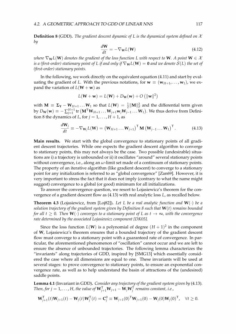
4.2. A GEOMETRIC APPROACH TO GDD OF LINEAR NNS 117
Definition 8 (GDD). The gradient descent dynamic of L is the dynamical system defined on Xby
dWdt
= −∇WL(W) (4.12)
where ∇WL(W) denotes the gradient of the loss function L with respect to W. A point W ∈ Xis a (first-order) stationary point of L if and only if ∇WL(W) = 0 and we denote S(L) the set of(first-order) stationary points.
In the following, we work directly on the equivalent equation (4.11) and start by eval-uating the gradient of L. With the previous notations, for w ≡ (wH+1, . . . , w1), we ex-pand the variation of L(W + w) as
L(W + w) = L(W) + DW(w) + O(‖w‖2)
with M ≡ ΣY −WH+1 . . . W1 so that L(W) = 12‖M‖2
F and the differential term givenby DW(w) ≡ −∑H+1
j=1 tr(MTWH+1 . . . Wj+1wjWj−1 . . . W1
). We thus derive from Defini-
tion 8 the dynamics of L, for j = 1, . . . , H + 1, as
dWj
dt≡ −∇Wj L(W) =
(WH+1 . . . Wj+1
)T M(Wj−1 . . . W1
)T . (4.13)
Main results. We start with the global convergence to stationary points of all gradi-ent descent trajectories. While one expects the gradient descent algorithm to convergeto stationary points, this may not always be the case. Two possible (undesirable) situa-tions are i) a trajectory is unbounded or ii) it oscillates “around” several stationary pointswithout convergence, i.e., along an ω-limit set made of a continuum of stationary points.The property of an iterative algorithm (like gradient descent) to converge to a stationarypoint for any initialization is referred to as “global convergence” [Zan69]. However, it isvery important to stress the fact that it does not imply (contrary to what the name mightsuggest) convergence to a global (or good) minimum for all initializations.
To answer the convergence question, we resort to Lojasiewicz’s theorem for the con-vergence of a gradient descent flow as (4.13) with real analytic loss L, as recalled below.
Theorem 4.3 (Lojasiewicz, from [Loj82]). Let L be a real analytic function and W(·) be asolution trajectory of the gradient system given by Definition 8 such that W(t) remains boundedfor all t ≥ 0. Then W(·) converges to a stationary point of L as t → ∞, with the convergencerate determined by the associated Lojasiewicz component [DK05].
Since the loss function L(W) is a polynomial of degree (H + 1)2 in the componentof W, Lojasiewicz’s theorem ensures that a bounded trajectory of the gradient descentflow must converge to a stationary point with a guaranteed rate of convergence. In par-ticular, the aforementioned phenomenon of “oscillation” cannot occur and we are left toensure the absence of unbounded trajectories. The following lemma characterizes the“invariants” along trajectories of GDD, inspired by [SMG13] which essentially consid-ered the case where all dimensions are equal to one. These invariants will be used atseveral stages: to prove convergence to stationary points, to ensure an exponential con-vergence rate, as well as to help understand the basin of attractions of the (undesired)saddle points.
Lemma 4.1 (Invariant in GDD). Consider any trajectory of the gradient system given by (4.13).Then, for j = 1, . . . , H, the value of WT
j+1Wj+1 −WjWTj remains constant, i.e.,
WTj+1(t)Wj+1(t)−Wj(t)WT
j (t) = C0j ≡ Wj+1(0)TWj+1(0)−Wj(0)Wj(0)T, ∀t ≥ 0.

118 CHAPTER 4. GRADIENT DESCENT DYNAMICS IN NEURAL NETWORKS
In particular, in the case of H = 1 we get WT2 W2 −W1WT
1 = C0 ≡ (WT2 W2 −W1WT
1 )∣∣t=0.
Proof. Simply check that ddt
(WT
j+1Wj+1 −WjWTj
)= 0.
Note in particular that, as a result of Lemma 4.1, there exists constant cj, 1 ≤ j ≤ Hsuch that for all t ≥ 0,
‖Wj+1(t)‖2F − ‖Wj(t)‖2
F = cj (4.14)
i.e., the difference between the (Frobenius) norms of successive weight matrices Wj arepreserved along with the gradient descent process.
With the key Lemma 4.1 and the remark above, to prove the boundedness of Wj(t)for all j = 1, . . . , H + 1, it suffices to bound any single one of them, say for j = H + 1. Tothis end, first note that
‖WH+1 . . . W1‖2F = tr(WT
H+1WH+1 . . . W2W1WT1 WT
2 . . . WTH)
= tr(WTH+1WH+1 . . . (W2WT
2 )2 . . . WT
H)− tr(WTH+1WH+1 . . . W2C0
1WT2 . . . WT
H)
together with the fact that for symmetric positive semi-definite A we have λmin(B) tr(A) ≤tr(AB) ≤ λmax(B) tr(A) so that
| tr(WTH+1WH+1 . . . W2C0
1WT2 . . . WT
H)| ≤ ‖C01‖‖WH+1 . . . W2‖2
F
so that by successively applying Lemma 4.1 one deduces the following bound
Pl(WH+1) ≤ ‖WH+1 . . . W1‖2F ≤ ‖Pu(WH+1)
for some polynomial Pl and Pu of degree H + 1 with positive leading coefficients. As aconsequence, by considering the time derivative of ‖WH+1‖2
F, one can similarly get
d‖WH+1‖2F
dt≤ −2C0‖WH+1‖2(H+1)
F + C1(1 + ‖WH+1‖2HF )
for some positive constants C0 and C1, so that d‖WH+1‖2F
dt < 0 for some ‖WH+1‖2F large
enough and WH+1 remains bounded for t ≥ 0 and this holds for all Wj, j = 1, . . . , H + 1via (4.14). As such, by Lojasiewicz’s theorem one achieves the global convergence tostationary points, stated as below.
Proposition 4.1 (Global convergence to stationary points). Let (X, Y) be a data-target pairsatisfying Assumptions 10 and 11. Then, every GDD trajectory defined in Definition 8 convergesto a (first-order) stationary point as t → ∞, at rate at least t−α, for some fixed α > 0 onlydepending on the problem.
As another important byproduct of Lemma 4.1, we have the following corollary thatensures an exponential convergence with a critical initialization scheme, and perhapsmore importantly, to convergence to the global minima with L = 0.
Corollary 4.1 (Exponential convergence with critical initialization). Let Assumptions 10 and 11hold. If we have in addition that d1 ≥ d2 ≥ . . . ≥ dH and the initialization
C0j ≡ Wj+1(0)TWj+1(0)−Wj(0)Wj(0)T ∈ Rdj×dj
has at least dj+1 positive eigenvalues, i.e., λdj+1(C0j ) > 0 for j = 1, . . . , H. Then, every trajectory
of the GDD converges to a global minimum at least at the rate of exp(−2αt), for some α > 0.

4.2. A GEOMETRIC APPROACH TO GDD OF LINEAR NNS 119
Proof. Recall the definition M = ΣY −WH+1 . . . W1 and consider its time derivative as
dMdt
= −H+1
∑j=1
WH+1 . . . Wj+1dWj
dtWj−1 . . . W1
= −H+1
∑j=1
WH+1 . . . Wj+1WTj+1 . . . WT
H+1MWT1 . . . WT
j−1Wj−1 . . . W1
so that
dLdt
=d‖M‖2
Fdt
= −2H+1
∑j=1
tr(
MTWH+1 . . . Wj+1WTj+1 . . . WT
H+1MWT1 . . . WT
j−1Wj−1 . . . W1
)≤ −2
H+1
∑j=1
j−1
∏k=1
λmin(WTk Wk) tr
(MTWH+1 . . . Wj+1WT
j+1 . . . WTH+1M
)≤ −2
H+1
∑j=1
j−1
∏k=1
λmin(WTk Wk)
H+1
∏l=j+1
λmin(WlWTl )‖M‖2
F
where we constantly use the fact that for symmetric and positive semi-definite A we have| tr(AB)| ≥ λmin(B) tr(A). Therefore, if there exists at least 1 ≤ j ≤ H + 1 such that
H+1
∏l=j+1
λmin(WlWTl )
j−1
∏k=1
λmin(WTk Wk) > 0 (4.15)
then we obtain d‖M‖2F
dt ≤ −C‖M‖2F for some C > 0 and thus the conclusion. To this end,
we derive, from Lemma 4.1 and Weyl’s inequality (see Lemma 2.10) that, for j = 1, . . . , H
λi(WTj+1Wj+1) ≥ λi(C0
j ) + λmin(WjWTj ) ≥ λi(C0
j ), i = 1, . . . , dj
with λi(C0j ) the i-th eigenvalue of C0
j arranged in nondecreasing order so that λ1(C0j ) =
λmin(C0j ). Then since d1 ≥ . . . ≥ dj ≥ dj+1 ≥ . . . ≥ dH, the matrix WT
j+1Wj+1 ∈ Rdj×dj isof rank maximum dj+1 and thus admits at least dj − dj+1 zero eigenvalues so that
λi(WTj+1Wj+1) = 0, λi(C0
j ) ≤ 0
for i = 1, . . . , dj − dj+1. Moreover, since for i = 1, . . . , dj+1 we also have,
λi+dj−dj+1(WTj+1Wj+1) = λi(Wj+1WT
j+1)
we further deduce that for i = 1, . . . , dj+1,
λi(Wj+1WTj+1) = λi+dj−dj+1(W
Tj+1Wj+1) ≥ λi+dj−dj+1(C
0j )
so that by taking j = 1 in (4.15) we result in
H
∏l=1
λmin(Wl+1WTl+1) ≥
H
∏l=1
λdl−dl+1+1(C0l ) ≡ α > 0
which concludes the proof.

120 CHAPTER 4. GRADIENT DESCENT DYNAMICS IN NEURAL NETWORKS
Remark 4.1 entails that, for a linear network, although in general only polynomialconvergence rate can be established, it is possible to wisely initialize the gradient descentalgorithm to achieve exponential convergence.
Apart from the critical initialization scheme proposed in Corollary 4.1 that leads to aglobal convergence to global minima, Proposition 4.1 itself does not guarantee the “qual-ity” of stationary point to which the trajectory converges.
In the following, we move on to consider the general situation that we initialize thegradient descent algorithm from a arbitrary point in the network weight space X andfocus on the set of the first-order stationary points S . We consider for simplicity the caseH = 1 and comment on H > 1.
Proposition 4.1 ensures, for all initializations, the convergence of the gradient de-scent to a stationary point, i.e., a point W in the state space X verifying ∇WL(W) = 0.Nonetheless, the information on the “quality” (e.g., the loss value L) of the solutionachieved is still unknown. To obtain a clearer picture, we now consider the case H = 1and focus on the set of all stationary points by further decomposing the loss L withΣY ≡
[SY 0
]for diagonal SY ∈ Rdy×dy with [SY]ii > 0 as
L(W1, W2) =12‖ΣY −W2W1‖2
F =12‖SY − CA‖2
F +12‖CB‖2
F (4.16)
with C ≡ W2 ∈ Rdy×d1 , A ∈ Rd1×dy and B ∈ Rd1×(dx−dy) such that[
A B]≡ W1.
Under the notations above, we further expand L(W + w) to obtain its higher ordervariation as
L(A + a, B + b, C + c) ≡ L(W + w) = L(W) + DW(w) + HW(w) + O(‖w‖3)
with M ≡ SY − CA, L(W) = 12‖M‖2
F +12‖CB‖2
F and
DW(w) ≡ − tr(
MT(Ca + cA))+ tr
(BTCT(Cb + cB)
)= O(‖w‖)
HW(w) ≡ − tr(MTca) +12‖Ca + cA‖2
F + tr(BTCTcb) +12‖Cb + cB‖2
F = O(‖w‖2)
that give the differential and the Hessian of L, respectively. Recall that S(L) ≡ W | DW(w) =0 and denote M ≡ SY − CA, so that, by Definition 8,
dAdt = CTM = 0dBdt = −CTCB = 0dCdt = MAT − CBBT = 0
⇔
CTSY = CTCACB = 0ASY = AATCT.
(4.17)
Observing the symmetric structure of A, C in (4.17) we have the following lemma.
Lemma 4.2 (Same kernel for A and CT). Let Assumptions 10 and 11 hold. Then for allW ∈ S(L),
ker A = ker CT, with ker A ≡ x, Ax = 0.Moreover, denote r the common rank of A and C with 0 ≤ r ≤ dy. Then there exists someorthogonal matrix U ∈ Rdy×dy such that
AU =[
A 0d1×(dy−r)
]CTU =
[CT 0d1×(dy−r)
]U−1SYU = SY
(4.18)

4.2. A GEOMETRIC APPROACH TO GDD OF LINEAR NNS 121
with A, CT ∈ Rd1×r. Moreover, if SY has distinct eigenvalues (i.e., Y has dy distinct singularvalues, as demanded in Assumption 12), then U is a diagonal matrix made of 1 and −1.
Sketch of proof of Lemma 4.2. It can be shown with basic algebraic manipulations that theeigenvectors of S2
Y (thus of SY) form a basis of both ker A and ker CT. Therefore ker A =ker CT and in particular dim ker A = dim ker CT. We denote this dimension dy − r andA, C are thus both of rank r. Choose U2 from ker A and U1 ⊥ ker A; we deduce U =[
U1 U2]
so that (4.18) holds.
In the general case H ≥ 1, similar conclusion as in Lemma 4.2 holds for the matrixproduct (WH+1 . . . W2)T and WH+1 . . . W2A for W1 ≡
[A B
].
Remark from (4.18) in Lemma 4.2 that, for arbitrary SY, there are infinitely manypossibilities on the choice of U with the risk of occupying too much of the state space X ,since, with the change of variable in Lemma 4.2 the state variable now becomes the tuple(A, B, C, U). Using Assumption 12, U only takes a finite number of values for a givenW ∈ Sr(L), hence the state variable essentially becomes the tuple (A, B, C).
For W ∈ S(L) with A, C of rank r with 0 ≤ r ≤ dy, rewriting SY in two blocks
SY =
[DY 00 EY
], with DY ∈ Rr×r and EY ∈ R(dy−r)×(dy−r). With Lemma 4.2, we then
simplify (4.17) as C A = DY
CB = 0, UTMU =
[0 00 EY
](4.19)
with the fact that CT, A are both of full rank (equal to r). The loss L(W) (at stationarypoints) can thus be simplified as L(W) = 1
2‖EY‖2F where EY measures the “quality” of
each stationary points.For any W ∈ S(L), with Lemma 4.2 we are allowed to “extract” the full rank (sub-
)structures of A, C with SY unchanged, via a simple change of basis. For 0 ≤ r ≤ dy, letSr(L) be the subset of S(L) such that the rank of A and of C is equal to r. Then, one hasthe following disjoint union
S(L) = ∪dyr=0Sr(L).
Proposition 4.2 (Landscape of single-hidden-layer linear NN model). Under Assump-tions 10–12, the loss function L(W) has the following properties:
1. The set of possible limits of L along the GDD given by (4.12) is equal to the finiteset made of the sum of the squares of any subset of the singular values of Y.
2. The set Sdy(L) is in fact the set of local (and global) minima, with L = 0 and M = 0.
3. Every first-order stationary point W ∈ Sr(L) with 0 ≤ r ≤ dy − 1 is a saddle pointsuch that the Hessian has at least one negative eigenvalue. In particular, the setof saddle points is an algebraic variety of positive dimension, i.e., (up to a unitarymatrix) the zero set of the polynomial functions given in (4.19), with EY 6= 0.
For more general DNNs with H > 1, similar conclusion holds, except from the neg-ative eigenvalue of the Hessian for all saddle points. As a matter of fact, for H > 1,there exists saddle points with positive semidefinite Hessian and we show that a suffi-cient condition to ensure at least one negative eigenvalue is to have rank(WH . . . W2) >rank(WH+1 . . . W2).
The fact that all local minima are equivalently global minima and all critical pointsthat are not global minima are saddle points with at least one negative eigenvalue for the

122 CHAPTER 4. GRADIENT DESCENT DYNAMICS IN NEURAL NETWORKS
Hessian is in fact already known for single-hidden-layer linear networks [BH89, Kaw16].Here, we improve the condition given in [Kaw16], with an alternative and shorter proofbased only on the quadratic form involving the Hessian, for deep linear networks.
With Proposition 4.2, and assume in addition that the loss function L admits two bytwo distinct values over two by two distinct subsets made of (the sum of the squares of)the singular values of the target Y, one is able to provide a precise “local” descriptionof all saddle points. Based on this description, one is able to further construct the lo-cal stable and unstable manifolds, with the help of the notation of normally hyperbolic[HPS06, Theorem 3.5]. Ultimately, with the fact that the loss value L is decreasing alongthe gradient descent trajectory and by contradiction, one reaches the convergence of theGDD trajectory to a global minima, from almost all initialization (in the sense of Lebesguemeasure).
Conclusion. The essential difference between the case H = 1 and deeper NN withH > 1 is the existence of saddle points with positive semidefinite Hessian matrices. Inthis case, one has to evaluate higher order information (≥ 3) to understand more pre-cisely the basins of attraction of these undesired stationary points, or otherwise establishtighter bounds for the dimension of the parameter space X that is occupied by these badsaddle points and their basins of attraction. Alternatively, one may also wish to provideinitialization scheme, in this H > 1 case, that can avoid, at least with high probability say,these bad saddle points, so that we can again apply the arguments as in the case H = 1.

Chapter 5
Conclusions and Perspectives
5.1 Conclusions
Under a simple GMM for the input data model, we investigated, in Section 3.1.1-3.2.2the performance of three closely connected objects: large random kernel matrices, largedimensional random feature maps, and large simple neural networks random weights.In the setting where the number of data n and their dimension p are both large and com-parable, the MSE of random neural networks, the misclassification error rate of kernelridge regression, as well as the performance of kernel/random feature-based spectralclustering techniques, all depend heavily on the eigenspectrum or on a functional of aparticular random kernel/nonlinear Gram matrix. The major technical challenge to the-oretically grasp these kernel matrices, so as to assess the performance of the aforemen-tioned algorithms, lies in the presence of nonlinearities, e.g., the kernel function f andthe neural network activation function σ. To handle this difficulty, we placed ourselvesunder the critical regime of asymptotically non-trivial classification (namely, Assump-tion 2 in Section 1.2). In this regime, a “concentration” phenomenon emerges, for thesimilarly measures ‖xi− xj‖2/p or xTi xj/p, which then helps (asymptotically) “linearize”(or Taylor-expand to first orders) the nonlinear objects of interest. The associated eigen-spectrum, therefore, behaves like (a scaled and shifted version of) the classical samplecovariance/Gram matrix, perturbed by low rank matrices, and only depends on the lo-cal behavior of the nonlinear function at the “concentration” point.
This “concentration” effect, if theoretically convenient, however, hinders the full dis-criminative power of kernels (such as the discrimination of covariance matrices in differ-ent classes). To work this limitation around, a proper scaling as xTi xj/
√p is necessary,
which we studied in the second part of the thesis. In this situation, a “concentration”cannot be established so that, in place of Taylor expansion arguments, we exploited themethod of orthogonal polynomials to decompose the nonlinear f into the sum of a lin-ear and a purely nonlinear parts, that both contribute to the kernel eigenspectrum, butin a very different way. A surprising outcome is that the kernel matrix eigenspectrumdepends on f solely via its first three Hermite coefficients, suggesting that, even with-out concentration, the space of kernel functions can be mapped to a low dimensionalsubspace. Similar behavior is also observed for the empirical risk-based classifier in Sec-tion 3.3, where the performance only depends on the loss function L through the samethree coefficients of the implicit proximal function. However, the performance descrip-tion in Section 3.3 is more complicated and can only be expressed as the fixed point of asystem of nonlinear equations. RMT analyses allow for direct access to the (asymptotic)performance of the aforementioned machine learning methods, so long as their solutions
123

124 CHAPTER 5. CONCLUSIONS AND PERSPECTIVES
are explicit or implicitly determined by (convex) optimization problems.
Aiming to study the impact of optimization algorithm in convex or non-convex prob-lems, we considered in Section 4.1 the temporal evolution of a single-layer linear neuralnetwork, learned by the gradient descent method, still under a GMM for the input data.Despite being a linear classifier, the training and test performance of this linear regres-sion model is a highly nonlinear function of the training time and involves the sum ofa nonlinear function of all the eigenvalues of the input covariance matrix. Based on theproposed RMT analysis, both the training and test performance of the model can be fullycharacterized in the large n, p limit. This result provides a first precise description of largenetwork performances when trained with gradient descent and sheds new light on manycommon questions in neural networks, such as overfitting, early stopping and the initial-ization of training, in the large dimensional regime where n, p→ ∞ with p/n→ c > 0.
When the number of hidden layers is more than one, the underlying optimizationproblem to train the neural network becomes non-convex and less tractable. In Section 4.2we took a geometric and, so far, only deterministic approach to understand the conver-gence properties of simple gradient descent algorithms in this problem. We improved theexisting analysis of the gradient descent dynamics in single-hidden-layer linear neuralnetworks by considering the corresponding dynamical system. Based on a cornerstone“invariance” structure in the network weight space, we provided alternative and sim-pler proofs and removed some unnecessary assumptions from previous contributions toachieve the “almost sure” convergence to global minima.
5.2 Limitations and Perspectives
Yet, these findings are limited to the simple but seemingly restrictive Gaussian mixturemodeling of the data. In the following, we discuss some possible future research direc-tions, in the continuation of our preliminary findings.
Universality of RMT results in machine learning applications. As discussed in theproof of the Marcenko-Pastur law in Section 2.2.2, as well as in the “properly scaled”inner product kernel matrix in Section 3.1.2, by positioning ourselves under the large di-mensional setting where n, p are both large and comparable, many random matrix-basedanalyses, for linear or nonlinear models, lead to universal results, in the sense that theyhold as long as the (original) random matrix Z ∈ Rp×n has i.i.d. zero mean and unitvariance entries, and are independent of the higher order statistics. Since real data gener-ally do not comply with this stringent i.i.d. assumption, it is of interest to investigate thelimitation of this universality phenomenon in machine learning applications. It is worthpointing out that the universality has already been observed to collapse in many nonlin-ear models, for instance in the “improperly scaled” shift-invariant kernel f (‖xi− xj‖2/p)investigated in [CBG16] where, by considering non-Gaussian Z with a non-zero excesskurtosis κ = E[Z4
ij]− 3 6= 0, the random variable ψi ≡ ‖ωi‖2 −E[‖ωi‖2] yields a differ-ent (statistical) behavior, which nonetheless only moderately impacts the performances ofkernel spectral clustering and kernel ridge regression methods. In [LLC18, BP19] whereone considers the Gram matrix σ(WX)Tσ(WX) in a random neural network context, ithas been observed that the higher order moments of the distribution of (the i.i.d. entriesof) the weight matrix W has an important impact on the eigenspectrum of the Gram ma-trix and consequently on the performance of the resulting neural network model. In thisrespect, one may wonder on the possibility to identify machine learning methods that

5.2. LIMITATIONS AND PERSPECTIVES 125
are “universal” and depend only on the first several moments of the data distributionfrom those that depend on the higher order moments of the data modeling. From a prac-tical standpoint, it is perhaps of more importance to empirically investigate which taskscan be sufficiently well fulfilled by only considering the first and second order informa-tion from the data. For non-universal models, a possible idea is to perform preliminarystudies on the influence of higher order information, starting from a qualitative study,so as to understand the (systematic) advantage of certain machine learning methods insome specific (e.g., kurtosis-sensitive) applications to provide theoretical guarantees ofthe existing algorithms as well as new insights in designing more efficient techniques.
RMT-based analyses of optimization problems. The random matrix analyses of opti-mization problems developed in this thesis are twofold:
1. As in Section 3.3, by considering the optimality condition of convex or non-convexoptimization problems (e.g., first- or second-order stationary points condition), RMTanalyses provide statistical descriptions of the local or global optima, which furtherlead to a theoretical understanding of the algorithm performance as well as a bet-ter hyperparameter tuning or “unbiasing” for these methods, as discussed at theend of Section 3.3. This scheme mainly works for convex (or strongly convex) opti-mization problems as in Section 3.3, where the uniqueness of the optimal solutionis naturally guaranteed.
2. For non-convex optimization problems as the single-hidden-layer neural networksstudied in Section 4.2, there may exist in general a large or even infinite number offirst or higher order stationary points. In this case, even if one manages to establishan almost sure global convergence to global minima, the rate of convergence can beextremely slow due to the presence of (possibly numerous) saddle points [DJL+17].A wisely chosen initialization (as proposed in Corollary 4.1) within a locally convexstructure helps accelerate the convergence rate, up to linear/exponential. This iswhere a RMT analysis may serve practical purposes: by leveraging the random na-ture of many non-convex optimization problems (e.g., with sensing matrices havingi.i.d. standard Gaussian entries [CP11a] or with random measurement of randomsignals in phase retrieval [CC15]), it is possible to propose the following two-stepalgorithms:
• initialization, that makes a RMT-based initial guess so as to start the gradientdescent away from any saddle points and within the “local valleys” of local(and global) minima;
• iterative refinement based on the gradient method, without leaving the initialvalley.
In this case, the convergence rate relies heavily on a proper initialization, that canbe achieved by means of spectral methods, e.g., to initialize with the top eigen-vectors of a carefully designed matrix, as in the case of phase retrieval, matrixsensing/completion and many others [CLC18]. In many cases, by considering astatistical modeling of the problem with repeated and informative patterns, it ispossible to construct a data-dependent (random) matrix M that follows a spikedmodel as discussed at length in Section 2.3. The RMT analysis can then be appliedto capture the statistical behavior of the top eigenvectors (that correspond to theisolated eigenvalues) of M, so as to measure the “distance” between the proposed

126 CHAPTER 5. CONCLUSIONS AND PERSPECTIVES
(spectral-based) initialization and the desired global minima. In this regard, RMToffers not only a powerful initialization scheme by proposing an optimal design forM, but also a precise description of the conditions under which the proposed ini-tialization works, by establishing “phase transition” conditions as discussed at theend of Section 2.3.
As a closing remark, in the regime where n, p, N are all large and comparable, withN the number of model parameters, many counterintuitive phenomena arise (recall fromFigure 1.5 that for N > n the test error decreases as the ratio N/n increases), for which weneed a deeper theoretical understanding. Indeed, modern machine learning systems areoften highly over-parameterized and it is an everyday occurrence in modern DNNs to haveN > max(n, p). As a consequence, random matrix-based approaches are a promisingtool to investigate these modern over-parameterized learning systems that are of greaterimportance today.

Appendix A
Mathematical Proofs
A.1 Proofs in Chapter 3
A.1.1 Intuitive calculus for Theorem 1.2
In this section we consider the empirical spectral measure of the following inner-productkernel matrix as in (1.13)
Kij =
f (xTi xj/
√p)/√
p for i 6= j0 for i = j
for independent random vector xi ∼ N (0, Ip) and in particular, the associated Stieltjestransform (see Definition 6) given by
m(z) ≡ 1n
tr Q(z), Q(z) ≡ (K− zIn)−1 .
Our objective here is to prove that m(z) is the (unique) solution of the following cubicequation
− 1m(z)
= z +a2
1m(z)c + a1m(z)
+ν− a2
1c
m(z)
with a1 = E[ξ f (ξ)] and ν = Var[ f (ξ)] ≥ a21 for standard Gaussian ξ ∼ N (0, 1).
Basic settings and notations. Following the ideas of the sample covariance model inSection 2.2.3, we remove the i-th row and the i-th column of the symmetric matrix Ksuch that
K =
[K−i f (XT
−ixi/√
p)/√
pf (xTi X−i/
√p)/√
p 0
], K−i = f (XT
−iX−i/√
p)/√
p ∈ R(n−1)×(n−1)
with zero on the diagonal of K−i and X−i ∈ Rp×(n−1) the data matrix without xi. As such,we have that K−i is independent of xi. We similarly define the resolvent Q−i of K−i as
Q−i = (K−i − zIn−1)−1
so that under the above notations, the (i, i)-th (diagonal) entry of Q is given by
Qii =1
−z− 1p f (xTi X−i/
√p)Q−i f (XT
−1xi/√
p)(A.1)
127

128 APPENDIX A. MATHEMATICAL PROOFS
where we recall that the diagonal of both K and K−i contain only zero entries. Sincewe are interested in the Stieltjes transform m(z) = 1
n ∑ni=1 Qii(z), the key object is the
(nonlinear) quadratic form 1p f (xTi X−i/
√p)Q−i f (XT
−1xi/√
p).To handle the nonlinear random vector f (XT
−ixi/√
p), we follow [CS13] and performthe following orthogonal decomposition of xj: for all j 6= i,
xj = αjxi
‖xi‖+ x⊥j (A.2)
where xi‖xi‖ is the unit vector in the direction of xi and x⊥j lies in the (p− 1)-dimensional
subspace orthogonal to xi. By orthogonality between x⊥j and xi we have
xTi xj/√
p = αj‖xi‖/√
p⇔ αj =xTi xj
‖xi‖
for j 6= i. Since xi and xj are independent standard Gaussian vectors, we have, in the largep limit that xTj xi/
√p ∼ N (0, 1) and ‖xi‖ '
√p. Moreover, αj ∼ N (0, 1), x⊥j ∼ N (0, Ip−1)
and both are decorrelated thus independent.Indeed,
Exj [αix⊥j ] = Exj
[xTi xj
‖xi‖
(xj −
xixTi xj
‖xi‖2
)]= Exj
[xjxTj xi
‖xi‖
]−Exj
[xixTi xjxTj xi
‖xi‖3
]= 0.
As such, we have for k 6= j, k 6= i that
xTj xk = αjαk + (x⊥j )Tx⊥k ≡ αjαk + Φ⊥jk (A.3)
where the cross terms disappear again by orthogonality. Note from (A.2) that with highprobability, both xj and x⊥j are of (Euclidean) norm O(
√p) while αj = O(1), Similarly,
in (A.3), both xTj xk and Φ⊥jk are of order O(√
p), while αjαk = O(1). In this sense, Φ⊥jkis asymptotically close to the inner product xTj xk, with only the contribution from xi ex-cluded and explicitly given by αjαk.
We further denote α−i =[α1, . . . , αi−1, αi+1, . . . , αn
]T ∈ Rn−1 and K⊥−i ∈ R(n−1)×(n−1)
with (j, k) entry given by
[K⊥−i]jk ≡ δj 6=k f((x⊥j )
Tx⊥k /√
p)
/√
p = δj 6=k f (Φ⊥jk/√
p)/√
p (A.4)
so that f (XT−ixi/
√p) ' f (α−i) in the sense that ‖ f (XT
−ixi/√
p) − f (α−i)‖/√
p → 0 asp→ ∞.
It is worth remarking here that, intuitively speaking, the random vector α−i is merelya standard Gaussian random vector α−i ∼ N (0, In−1) in the large n, p limit in the sensethat its each entry is “asymptotically” Gaussian and uncorrelated with each other.
The advantage of introducing Φ⊥ (as well as K⊥−i) is that α−i is “essentially” asymp-totically independent of Φ⊥ in the sense that the expectation E[Φ⊥α−i] asymptoticallyvanishes. Note that this is in particular not the case for E[K−iα−i] as an instance.
Since the study of K−i boils down to that of K⊥−i, we will need in the remainder itsresolvent
Q⊥−i ≡(
K⊥−i − zIn−1
)−1
the resolvent of K⊥−i that is therefore also independent of α−i.

A.1. PROOFS IN CHAPTER 3 129
Nonlinear quadratic forms. We first focus on K−i ∈ R(n−1)×(n−1). By (A.3), the (k, l)-entry of K−i ≡ f (XT
−iX−i/√
p)/√
p is given by
[K−i]jk =1√
pf(
1√
pαjαk +
1√
pΦ⊥jk
)where we recall that Φ⊥jk/
√p = O(1), αjαk/
√p = O(p−1/2) and they are independent.
As a consequence, with a Taylor expansion of f(
1√p αjαk +
1√p Φ⊥jk
)around the dominant
Φ⊥jk/√
p we obtain1
f(
1√
pαjαk +
1√
pΦ⊥jk
)= f
(1√
pΦ⊥jk
)+ f ′
(1√
pΦ⊥jk
)1√
pαjαk + O(p−1)
so that in matrix form
[K−i]jk =1√
pf(
1√
pαjαk +
1√
pΦ⊥jk
)=
1√
pf(
1√
pΦ⊥jk
)+
1p
a1αjαk +1p
g(
1√
pΦ⊥jk
)αjαk + O(p−3/2)
= [K⊥−i]jk +1p
a1
(α−iα
T−i − diag(α2
−i))
jk+
1p(diag(α−i)G diag(α−i))jk + O(p−3/2)
where we denote the shortcut g(x) = f ′(x)− a1, for K⊥−i given by (A.4), [α2−i]j = α2
j and
G ≡ g(Φ⊥/√
p) ∈ R(n−1)×(n−1).The linear part a1x of the nonlinear function f (x) is treated separately since, intu-
itively speaking, taking the derivative of f (x) with a0 = 0 (see the last item of Assump-tion 3), results in E[ f ′(x)] = a1 6= 0. The fact that f ′(x) is not centered (with respectto the Gaussian measure), together with ‖α−i‖ = O(
√p), implies that a1
p α−iαT−i that has
non-vanishing operator norm as n, p→ ∞. By subtracting a1 from f ′(x), one obtains
[G/√
p]jk = δj 6=kg((x⊥j )
Tx⊥k /√
p)
/√
p.
Since the (original) kernel matrix K is of bounded operator norm for all f with a0 =E[ f (ξ)] = 0 and ξ ∼ N (0, 1) (see for a proof in [FM19, Theorem 1.7]), G/
√p, which
can be seen as another inner-product kernel matrix with centered kernel function g (withE[g(ξ)] = 0), has asymptotically bounded operator norm.
Further noting that diag(α−i) = O‖·‖(1), diag(α−i) = O‖·‖(1), we conclude that
K−i = K⊥−i +a1
pα−iα
T−i + o‖·‖(1) (A.5)
where o‖·‖(1) denotes a matrix with vanishing operator norm as n, p → ∞. Here we usethe fact that for A, B ∈ Rn×n, we have ‖AB‖ ≤ ‖A‖‖B‖ and ‖A‖ ≤ n‖A‖∞.
We now move on to the quadratic form 1p f (xTi X−i/
√p)Q−i f (XT
−1xi/√
p), for Q−i ≡(K−i − zIn−1)
−1. As a consequence of (A.5) we deduce
Q−i '(
K⊥−i +1p
a1α−iαT−i − zIn−1
)−1
= Q⊥−i −a1Q⊥−i
1p α−iα
T−iQ
⊥−i
1 + a1p αT−iQ
⊥−iα−i
' Q⊥−i −a1Q⊥−i
1p α−iα
T−iQ
⊥−i
1 + a1p tr Q⊥−i
' Q⊥−i −a1Q⊥−i
1p α−iα
T−iQ
⊥−i
1 + a− 1 np m(z)
1Here we consider for the moment f to be a Hermite polynomial, and then extend to square-summablef with Assumption 3.
130 APPENDIX A. MATHEMATICAL PROOFS
where we recall Q⊥−i ≡(K⊥−i − zIn−1
)−1 the resolvent of K⊥−i that is independent of α−i.Here we use Lemma 2.8 for the equality and Lemma 2.11 for the approximation in thesecond line.
With the approximation above and (A.2), the quadratic form of crucial interest can beexpanded as
1p
f (xTi X−i/√
p)Q−i f (XT−1xi/
√p) ' 1
pf (α−i)
TQ⊥−i f (α−i)− a1
(1p αT−iQ
⊥−i f (α−i)
)2
1 + a1np m(z)
' a21
pαT−iQ
⊥−iα−i +
1p
f>1(α−i)Q⊥−i f>1(α−i)− a1
(a1p αT−iQ
⊥−iα−i
)2
1 + a1np m(z)
where we write the Hermite polynomial f (x) as the sum of its linear part a1x and thepurely nonlinear part f>1(x) = f (x)− a1x that is orthogonal to x in the sense that Eξ [ξ f>1(ξ)] =0 for ξ ∼ N (0, 1). Again by orthogonality, the cross terms of α−i and f>1(α−i) vanish.Also, since
1p
f>1(α−i)Q⊥−i f>1(α−i) ' (ν− a21)
np
m(z)
one obtains the following approximation for the nonlinear quadratic form of interest
1p
f (xTi X−i/√
p)Q−i f (XT−1xi/
√p) '
a21
np m(z)
1 + a1np m(z)
+ (ν− a21)
np
m(z).
Ultimately with (A.1) one has
m(z) =1n
n
∑i=1
1−z− 1
p f (xTi X−i/√
p)Q−i f (XT−1xi/
√p)' 1
−z−a21c m(z)
1+ a1c m(z)
− ν−a21
c m(z).
which concludes the proof of Theorem 1.2.
A.1.2 Proof of Theorem 3.1
Our interest here is on the decision function of LS-SVM: g(x) = βTk(x) + b with (β, b)given by β = Q
(I− 1n1Tn Q
1Tn Q1n
)y
b = 1Tn Qy1Tn Q1n
and Q =(
K + nγ I)−1
.Before going into the detailed proof, as we will frequently deal with random variables
evolving as n, p grow large, we will use the extension of the O(·) notation introducedin [CBG16]: for a random variable x ≡ xn and un ≥ 0, we write x = O(un) if for anyη > 0 and D > 0, we have nDP(x ≥ nηun) → 0. Note that under Assumption 4 it isequivalent to use either O(un) or O(up) since n, p scale linearly. In the following we shalluse constantly O(un) for simplicity.
When multidimensional objects are concerned, v = O(un) means the maximum entryof a vector (or a diagonal matrix) v in absolute value is of order O(un) and M = O(un)means that the operator norm of M is of order O(un). We refer the reader to [CBG16] formore discussions on these practical definitions.

A.1. PROOFS IN CHAPTER 3 131
Under the growth rate settings of Assumption 4, from [CBG16], the approximation ofthe kernel matrix K is given by
K = −2 f ′(τ)(
PΩTΩP + A)+ βI + O(n−
12 )
with β = f (0)− f (τ) + τ f ′(τ) and A = An + A√n + A1, An = − f (τ)2 f ′(τ)1n1Tn and A√n, A1
given by (A.6) and (A.7) at the top of next page, where we denote
ta ≡tr(Ca − C)√
p= O(1), (ψ)2 ≡ [(ψ1)
2, . . . , (ψn)2]T.
A√n = −12
ψ1Tn + 1nψT +
ta
1na√p
2
a=11Tn + 1n
tb
1Tnb√p
2
b=1
(A.6)
A1 = −12
‖µa − µb‖
2 1na 1Tnb
p
2
a,b=1
−(ΩP)Ta (µb − µa)1
Tnb√
p
2
a,b=1
+
1na(µb − µa)
T(ΩP)b√p
2
a,b=1
− f ′′(τ)4 f ′(τ)
(ψ)21Tn + 1n[(ψ)2]T +
t2
a1na
p
2
a=11Tn + 1n
t2b
1Tnb
p
2
b=1
+ 2
tatb
1na 1Tnb
p
2
a,b=1
+ 2 diagtaIna2a=1ψ
1Tn√p+ 2ψ
tb
1Tnb√p
2
b=1
+ 21n√
p(ψ)T diagta1na2
a=1
+ 2
ta1na√
p
2
a=1(ψ)T + 4
tr(CaCb)
1na 1Tnb
p2
2
a,b=1
+ 2ψ(ψ)T
(A.7)
We start with the resolvent Q. The terms of leading order in K, i.e.,−2 f ′(τ)An and nγ I
are both of operator norm O(n). Therefore a Taylor expansion can be performed as
Q =
(K +
nγ
I)−1
=1n
[L−1 − 2 f ′(τ)
n
(A√n + A1 + PΩTΩP
)+
βIn
+ O(n−32 )
]−1
=Ln+
2 f ′(τ)n2 LA√nL + L
(B− β
n2 I)
L + O(n−52 )
with L =(
f (τ) 1n 1n1Tn + I
γ
)−1of order O(1) and B = 2 f ′(τ)
n2
(A1 + PΩTΩP + 2 f ′(τ)
n A√nLA√n
).
With the Sherman-Morrison formula we are able to compute explicitly L as
L =
(f (τ)
1n
1n1Tn +Iγ
)−1
= γ
(I− γ f (τ)
1 + γ f (τ)1n
1n1Tn
)=
γ
1 + γ f (τ)I +
γ2 f (τ)1 + γ f (τ)
P = O(1). (A.8)
Writing L as a linear combination of I and P is useful when computing L1n or 1Tn L,because by the definition of P = I− 1
n 1n1Tn , we have 1Tn P = P1n = 0.We shall start with the term 1Tn Q, since it is the basis of several other terms appearing
in β and b,
1Tn Q =γ1Tn
1 + γ f (τ)
[In+
2 f ′(τ)n2 A√nL +
(B− β
n2 I)
L]+ O(n−
32 )
132 APPENDIX A. MATHEMATICAL PROOFS
since 1Tn L = γ1+γ f (τ)1Tn .
With 1Tn Q at hand, we next obtain,
1n1Tn Q =γ
1 + γ f (τ)
[1n1Tn
n︸ ︷︷ ︸O(1)
+2 f ′(τ)
n2 1n1Tn A√nL︸ ︷︷ ︸O(n−1/2)
+ 1n1Tn
(B− β
n2 I)
L︸ ︷︷ ︸O(n−1)
]+ O(n−
32 ) (A.9)
1Tn Qy =γ
1 + γ f (τ)
[c2 − c1︸ ︷︷ ︸
O(1)
+2 f ′(τ)
n2 1Tn A√nLy︸ ︷︷ ︸O(n−1/2)
+ 1Tn
(B− β
n2 I)
Ly︸ ︷︷ ︸O(n−1)
]+ O(n−
32 ) (A.10)
1Tn Q1n =γ
1 + γ f (τ)
[1︸︷︷︸
O(1)
+2 f ′(τ)
n2
γ1Tn A√n1n
1 + γ f (τ)︸ ︷︷ ︸O(n−1/2)
+γ
1 + γ f (τ)1Tn
(B− β
n2 I)
1n︸ ︷︷ ︸O(n−1)
]+O(n−
32 ).
(A.11)The inverse of 1Tn Q1n can consequently be computed using a Taylor expansion around
its leading order, allowing an error term of O(n−32 ) as
11Tn Q1n
=1 + γ f (τ)
γ
[1︸︷︷︸
O(1)
− 2 f ′(τ)n2
γ1Tn A√n1n
1 + γ f (τ)︸ ︷︷ ︸O(n−1/2)
− γ
1 + γ f (τ)1Tn
(B− β
n2 I)
1n︸ ︷︷ ︸O(n−1)
]+O(n−
32 ).
(A.12)Combing (A.9) with (A.12) we deduce
1n1Tn Q1Tn Q1n
=1n
1n1Tn︸ ︷︷ ︸O(1)
+2 f ′(τ)
n2 1n1Tn A√n
[L−
γ 1n 1n1Tn
1 + γ f (τ)
]︸ ︷︷ ︸
O(n−1/2)
+ 1n1Tn
(B− β
n2 I) [
L−γ 1
n 1n1Tn1 + γ f (τ)
]︸ ︷︷ ︸
O(n−1)
+O(n−32 ) (A.13)
and similarly the following approximation of b as
b = c2 − c1︸ ︷︷ ︸O(1)
− 2γ√
pc1c2 f ′(τ)(t2 − t1)︸ ︷︷ ︸
O(n−1/2)
− γ f ′(τ)n
yTPψ︸ ︷︷ ︸O(n−1)
−γ f ′′(τ)2n
yTP(ψ)2 +4γc1c2
p[c1T1 + (c2 − c1)D− c2T2]︸ ︷︷ ︸
O(n−1)
+O(n−32 ) (A.14)
where
D =f ′(τ)
2‖µ2 − µ1‖
2 +f ′′(τ)
4(t1 + t2)
2 + f ′′(τ)tr C1C2
p
Ta = f ′′(τ)t2a + f ′′(τ)
tr C1C2
p
which gives the asymptotic approximation of b.

A.1. PROOFS IN CHAPTER 3 133
Moving to β, note from (A.8) that L− γ1+γ f (τ)
1n 1n1Tn = γP, and we can thus rewrite:
1n1Tn Q1Tn Q1n
=1n
1n1Tn +2γ f ′(τ)
n2 1n1Tn A√nP + γ1n1Tn
(B− β
n2 I)
P + O(n−32 ).
At this point, for β = Q(
I− 1n1Tn Q1Tn Q1n
)y, we have
β = Q[
I− 2γ f ′(τ)n2 1n1Tn A√n − γ1n1Tn
(B− β
n2 I) ]
Py + O(n−52 ).
Here again, we use 1Tn L = γ1+γ f (τ)1Tn and L− γ
1+γ f (τ)1n 1n1Tn = γP, to eventually get
β =γ
nPy︸︷︷︸
O(n−1)
+ γ2P(
B− β
n2 I)
Py︸ ︷︷ ︸O(n−2)
− γ2
1 + γ f (τ)
(2 f ′(τ)
n2
)2
LA√n1n1Tn A√nPy︸ ︷︷ ︸O(n−2)
+O(n−52 ).
(A.15)Note here the absence of a term of order O(n−3/2) in the expression of β since PA√nP = 0from (A.6).
We now work on the vector k(x) for a new datum x, following the same analysis as in[CBG16] for the kernel matrix K, assuming that x ∼ N (µa, Ca) and recalling the randomvariables definitions,
ωx ≡ (x− µa)/√
p
ψx ≡ ‖ωx‖2 −E‖ωx‖2.
We show that the j-th entry of k(x) can be written as
[k(x)]j = f (τ)︸︷︷︸O(1)
+ f ′(τ)[
ta + tb√p
+ ψx + ψj − 2(ωx)Tωj︸ ︷︷ ︸
O(n−1/2)
+‖µb − µa‖2
p+
2√
p(µb − µa)
T(ωj −ωx)︸ ︷︷ ︸O(n−1)
]
+f ′′(τ)
2
[ (ta + tb√
p+ ψj + ψx
)2
+4p2 tr CaCb︸ ︷︷ ︸
O(n−1)
]+ O(n−
32 ). (A.16)
Combining (A.15) and (A.16), we deduce
βTk(x) =2γ√
pc1c2 f ′(τ)(t2 − t1)︸ ︷︷ ︸
O(n−1/2)
+γ
nyTPk(x)︸ ︷︷ ︸O(n−1)
+γ f ′(τ)
nyTP(ψ− 2PΩTωx)︸ ︷︷ ︸
O(n−1)
+O(n−32 )
(A.17)with k(x) given as follows.

134 APPENDIX A. MATHEMATICAL PROOFS
k(x) = f ′(τ)‖µb − µa‖2
p1nb
2
b=1− 2 f ′(τ)√
p
1nb(µb − µa)
T2
b=1ωx
+2 f ′(τ)√
pdiag
(1nb(µb − µa)
T2
b=1Ω
)+
f ′′(τ)2
(ta + tb)
2
p1nb
2
b=1
+f ′′(τ)
2
[2 diag
(ta + tb√
p1nb
2
b=1
)ψ + 2
ta + tb√
p1nb
2
b=1ψx + (ψ)2 + 2ψxψ + ψ2
x1n
+
4p2 tr(CaCb)1nb
2
b=1
](A.18)
At this point, note that the term of order O(n−12 ) in the final object g(x) = βTk(x) + b
disappears because in both (A.14) and (A.17) the term of order O(n−1/2) is 2γ√p c1c2 f ′(τ)(t2−
t1) but of opposite signs. Also, we see that the leading term c2 − c1 in b will remain ing(x) as stated in Remark 3.1.
The development of yTPk(x) induces many simplifications, since i) P1n = 0 and ii)random variables as ωx and ψ in k(x), once multiplied by yTP, thanks to probabilisticaveraging of independent zero-mean terms, are of smaller order and thus become negli-gible. We thus get
γ
nyTPk(x) = 2γc1c2 f ′(τ)
[‖µ2 − µa‖2 − ‖µ1 − µa‖2
p− 2(ωx)
T µ2 − µ1√p
]+
γ f ′′(τ)2n
yTP(ψ)2
+ γc1c2 f ′′(τ)[
2(
ta√p+ ψx
)t2 − t1√
p+
t22 − t2
1p
+4p2 tr Ca(C2 − C1)
]+ O(n−
32 ). (A.19)
This result, together with (A.17), completes the analysis of the term βTk(x). Combin-ing (A.17)-(A.19) with (A.14) we conclude the proof of Theorem 3.1.
A.1.3 Proof of Theorem 3.2
This section is dedicated to the proof of the central limit theorem for
g(x) = c2 − c1 + γ (R+ cxD)
with the shortcut cx = −2c1c22 for x ∈ C1 and cx = 2c2
1c2 for x ∈ C2, and R,D as definedin (3.8) and (3.9).
Our objective is to show that, for a ∈ 1, 2, n(g(x)− Ga)→ 0 in distribution with
Ga ∼ N (Ga, VGa)
where Ga and VGa are given in Theorem 3.2. We recall that x = µa +√
pωx with ωx ∼N (0, Ca/p).
Letting zx such that ωx = C1/2a zx/
√p, we have zx ∼ N (0, I) and we can rewrite g(x)
in the following quadratic form (of zx) as
g(x) = zTx Azx + zTx b + c

A.1. PROOFS IN CHAPTER 3 135
with
A = 2γc1c2 f ′′(τ)tr(C2 − C1)
pCa
p
b = −2γ f ′(τ)n
(Ca)12
√p
ΩPy− 4c1c2γ f ′(τ)√
p(Ca)
12
√p
(µ2 − µ1)
c = c2 − c1 + γcxD− 2γc1c2 f ′′(τ)tr(C2 − C1)
ptr Ca
p.
Since zx is standard Gaussian and has the same distribution as Uzx for any orthogonalmatrix U (i.e., such that UTU = UUT = I), we choose U that diagonalizes A such thatA = UΛUT, with Λ diagonal so that g(x) and g(x) have the same distribution where
g(x) = zTx Λzx + zTx b + c =n
∑i=1
(z2
i λi + zi bi +cn
)and b = UTb, λi the diagonal elements of Λ and zi the elements of zx.
Conditioning on Ω, this results in the sum of independent but not identically dis-tributed random variables ri = z2
i λi + zi bi +cn . We then resort to the Lyapunov CLT
[Bil12, Theorem 27.3].We begin by estimating the expectation and the variance
E[ri|Ω] = λi +cn
Var[ri|Ω] = σ2i = 2λ2
i + b2i
of ri, so thatn
∑i=1
E[ri|Ω] = c2 − c1 + γcxD = Ga
s2n =
n
∑i=1
σ2i = 2 tr(A2) + bTb
= 8γ2c21c2
2(
f ′′(τ))2 (tr (C2 − C1))
2
p2tr C2
ap2
+ 4γ2(
f ′(τ)n
)2
yTPΩT Ca
pΩPy +
16γ2c21c2
2( f ′(τ))2
p(µ2 − µ1)
T Ca
p(µ2 − µ1) + O(n−
52 ).
We shall rewrite Ω into two blocks as:
Ω =
[(C1)
12√
p Z1, (C2)12√
p Z2
]where Z1 ∈ Rp×n1 and Z2 ∈ Rp×n2 with i.i.d. Gaussian entries with zero mean and unitvariance. Then
ΩT Ca
pΩ =
1p2
[ZT
1 (C1)12 Ca(C1)
12 Z1 ZT
1 (C1)12 Ca(C2)
12 Z2
ZT2 (C2)
12 Ca(C1)
12 Z1 ZT
2 (C2)12 Ca(C2)
12 Z2
]and with Py = y− (c2 − c1)1n, we deduce
yTPΩT Ca
pΩPy =
4p2
(c2
21Tn1ZT
1 (C1)12 Ca(C1)
12 bZ11n1
−2c1c21Tn1ZT
1 (C1)12 Ca(C2)
12 Z21n2 + c2
21Tn1ZT
2 (C2)12 Ca(C2)
12 Z21n2
).

136 APPENDIX A. MATHEMATICAL PROOFS
Since Zi1ni ∼ N (0, niIni), by applying the trace lemma (Lemma 2.11), we get
yTPΩT Ca
pΩPy− 4nc2
1c22
p2
(tr C1Ca
c1+
tr C2Ca
c2
)a.s.−→0. (A.20)
Consider now the events
E =
∣∣∣∣yTPΩT Ca
pΩPy− ρ
∣∣∣∣ < ε
E =
∣∣∣∣yTPΩT Ca
pΩPy− ρ
∣∣∣∣ > ε
for any fixed ε with ρ =4nc2
1c22
p2
(tr C1Ca
c1+ tr C2Ca
c2
)and write
E
[exp
(iun
g(x)− Ga
sn
)]= E
[exp
(iun
g(x)− Ga
sn
) ∣∣∣∣E] P(E)
+ E
[exp
(iun
g(x)− Ga
sn
) ∣∣∣∣E] P(E) (A.21)
We start with the variable g(x)|E and check that Lyapunov’s condition for ri = ri −E[ri],
limn→∞
1s4
n
n
∑i=1
E[|ri|4] = limn→∞
n
∑i=1
60λ4i + 12λ2
i bi2+ 3bi
4
s4n
= 0
since both λi and bi are of order O(n−3/2).As a consequence, we have the CLT for the random variable g(x)|E. Thus
E
[exp
(iun
g(x)− Ga
sn
) ∣∣∣∣E]→ exp(−u2/2).
Next, we see that the second term in (A.21) goes to zero because∣∣E[ exp
(iun g(x)−Ga
sn
) ∣∣E]∣∣ ≤1 and P(E)→ 0 from (A.20). We eventually deduce
E
[exp
(iun
g(x)− Ga
sn
)]→ exp(−u2/2).
With the help of Lévy’s continuity theorem, we thus prove the CLT of the variablen g(x)−Ga
sn. Since s2
n → VGa , with Slutsky’s theorem, we have the CLT for n g(x)−Ga√VGa
and
eventually for n g(x)−Ga√VGa
by Theorem 3.1 which completes the proof.
A.1.4 Proof of Proposition 3.2
We aim to prove, for f (x) = xk with k ≥ 2, the informative kernel matrix KI in Proposi-tion 3.2 defined as
KI =k√
p(ZTZ/
√p)(k−1) (A + B) +
k(k− 1)2√
p(ZTZ/
√p)(k−2) (A)2 (A.22)

A.1. PROOFS IN CHAPTER 3 137
for Aij ≡ δi 6=jzTi (Ea+Eb)zj
2√
p and Bij ≡ δi 6=jµT
a µb+µTa zj+µT
b zi√p − zTi (Ea−Eb)
2zj8√
p , has a tractable low-
rank approximation K given by
KI =
k!!p (JMTMJT + JMTZ + ZTMJT), for k odd;
k(k−1)!!2p J (T + S) JT, for k even.
(A.23)
Define by L the matrix with Lij ≡ [ 1p (JMTMJT + JMTZ + ZTMJT)]ij for i 6= j and
Lii = 0. Then KI can be written as
KI = k(ZTZ/√
p)(k−1) L + Φ,
Φij ≡kp(zTi zj/
√p)k−1zTi
(12(Ea + Eb)−
18(Ea − Eb)
2)
zj
+k(k− 1)
8p(zTi zj/
√p)k−2 1
√p(zTi (Ea + Eb)zj)
2
for i 6= j and Φii = 0. With this expression, the proof of Proposition 3.2 can be dividedinto three steps.
I. Concentration of Φ. We first show that ‖Φ−E[Φ]‖ → 0 almost surely, as n, p → ∞.This follows from the observation that Φ is a p−1/4 rescaling (since ‖Ea‖ = O(p−1/4)) ofthe null model KN , which concentrates around its expectation in the sense that ‖KN −E[KN ]‖ = O(1) for E[KN ] = O(
√p) if a0 6= 0 (see Remark 3.6). Indeed, it is shown
in [FM19, Theorem 1.7] that, the leading eigenvalue of order O(√
p) discarded (arisingfrom E[KN ]), KN is of bounded operator norm for all large n, p with probability one;this, together with the fact that ‖E[Φ]‖ = O(1) that will be shown subsequently (andindependently), allows us to conclude that ‖Φ−E[Φ]‖ → 0 as n, p→ ∞.
II.I Computation of E[Φ]: Gaussian case. Recall that the entries of Φ are the sum ofrandom variables of the type
φ =C√
p(xTy/
√p)α(xTFy)β
for independent random vectors x, y ∼ N (0, Ip) in the Gaussian case. As such, we resortto computing, as in [Wil97, LLC18] (or Section A.1.6), the integral
Ez[(zTa)k1(zTb)k2 ] = (2π)−p/2∫
Rp(zTa)k1(zTb)k2 e−‖z‖
2/2dz
=1
2π
∫R2(z1 a1)
k1(z1b1 + z2b2)k2 e−(z
21+z2
2)/2dz1dz2 =1
2π
∫R2(zTa)k1(zTb)k2 e−‖z‖
2/2dz
where we apply the Gram-Schmidt procedure to project z onto the two-dimensional
space2 spanned by a, b with a1 = ‖a‖, b1 = aTb‖a‖ , b2 =
√‖b‖2 − (aTb)2
‖a‖2 and denote
2By assuming first that a, b are linearly independent before extending by continuity to a, b proportional.

138 APPENDIX A. MATHEMATICAL PROOFS
z = [z1; z2], a = [a1; 0] and b = [b1; b2]. As a consequence, we obtain, for k even,
E[(zTi zj/
√p)k]= E[ξk] = (k− 1)!!;
Ezi
[(zTi zj/
√p)k(zTi b)
]= Ezi
[(zTi zj/
√p)k−1(zTi b)2
]= 0;
Ezi
[(zTi zj/
√p)k−1(zTi b)
]= (k− 1)!!(‖zj‖/
√p)k−2(zTj b)/
√p;
Ezi
[(zTi zj/
√p)k(zTi b)2
]= (k− 1)!!
(k(‖zj‖/
√p)k−2(zTj b/
√p)2 + (‖zj‖/
√p)k‖b‖2
);
where k!! is the double factorial of an integral k defined by k!! = k(k− 2)(k− 4) · · ·. Thisfurther leads, in the Gaussian case, to the expression of KI in Proposition 3.2.
II.II Computation of E[Φ]: beyond the Gaussian case. We then show that, for randomvectors z with zero mean, unit variance and bounded moments entries, the expressionof E[Φ] coincides with the Gaussian case. To this end, recall that the entries of Φ are thesum of random variables of the type
φ =C√
p(xTy/
√p)α(xTFy)β
for independent random vectors x, y ∈ Rp with i.i.d. zero mean, unit variance and finitemoments (uniformly on p) entries, deterministic F ∈ Rp×p, C ∈ R, α ∈N and β ∈ 1, 2.Let us start with the case β = 1 and expand φ as
φ =C√
p
(1√
p
p
∑i1=1
xi1 yi1
). . .
(1√
p
p
∑iα=1
xiαyiα
)(p
∑j1,j2=1
Fj1,j2 xj1 yj2
)(A.24)
with xi and yi the i-th entry of x and y, respectively, so that i) xi is independent of yj forall i, j and ii) xi is independent of xj for i 6= j with E[xi] = 0, E[x2
i ] = 1 and E[|xi|k] ≤ Ckfor some Ck independent of p (and similarly for y).
At this point, note that to ensure E[KI ] has non-vanishing operator norm as n, p→ ∞,we need E[φ] ≥ O(p−1) since ‖A‖ ≤ p‖A‖∞ for A ∈ Rp×p. Also, note that (as β = 1),all terms in the sum ∑
pj1,j2=1 Fj1,j2 xj1 yj2 with j1 6= j2 must be zero since in other terms
xi always appears together with yi, so that all terms with j1 6= j2 give rise to zero inexpectation. Hence, the p2 terms of the sum only contain p nonzero terms in expectation(those with j1 = j2). The arbitrary (absolute) moments of x and y being finite, the firstαp terms must be divided into dαe/2 groups of size two (containing O(p) terms) so that,with the normalization by p−1 for each group of size two, the associated expectation doesnot vanish. We thus discuss the following two cases:
1. α even: the α terms in the sum form α/2 groups with different indices each and alsodifferent from j1 = j2. Therefore we have Exj [φ] = 0.
2. α odd: the α terms in the sum form (α − 1)/2 groups with indices different fromeach other and the remaining one goes with the last term containing F and one hasE[φ] = Cα!!
p tr(F) by a combinatorial argument.
The case β = 2 follows exactly the same line of arguments except that j1 may not equal j2to give rise to non-vanishing terms.

A.1. PROOFS IN CHAPTER 3 139
III. Concentration of Hadamard product. It now remains to treat k(ZTZ/√
p)(k−1) Land show it also has an asymptotically deterministic behavior (as Φ). It can be shownthat
‖N L‖ → 0, n, p→ ∞
with N = (ZTZ/√
p)(k−1) − (k − 2)!!1n1Tn for k odd and N = (ZTZ/√
p)(k−1) for keven.
To prove this, note that, depending on the parameter a0 = E[ f (ξ)], the operator normof f (ZTZ/
√p)/√
p is either of order O(√
p) for a0 6= 0 or O(1) for a0 = 0. In particular,for monomials f (x) = xk under study here, we have a0 = E[ξk] = 0 for k odd anda0 = E[ξk] = (k− 1)!! 6= 0 for k even, ξ ∼ N (0, 1). To control the operator norm of theHadamard product between matrices, we introduce the following lemma.
Lemma A.1. For A, B ∈ Rp×p, we have ‖A B‖ ≤ √p‖A‖∞‖B‖.
Proof of Lemma A.1. Let e1, . . . , ep be the canonical basis vectors of Rp, then for all 1 ≤ i ≤p,
‖(A B)ei‖ ≤ maxi,j|Aij|‖Bei‖ = ‖A‖∞‖Bei‖ ≤ ‖A‖∞‖B‖.
As a consequence, for any v = ∑pi=1 viei, we obtain
‖(A B)v‖ ≤p
∑i=1|vi|‖(A B)ei‖ ≤
p
∑i=1|vi|‖A‖∞‖B‖
which, by Cauchy-Schwarz inequality further yields ∑pi=1 |vi| ≤
√p‖v‖. This concludes
the proof of Lemma A.1.
Lemma A.1 tells us that the Hadamard product between a matrix with o(p−1/2) entryand a matrix with bounded operator norm is of vanishing operator norm, as p → ∞. Assuch, since ‖N‖ = O(1) and L has O(p−1) entries, we have ‖N L‖ → 0. This concludesthe proof of Proposition 3.2.
A.1.5 Proof of Theorem 3.5
We aim to prove Theorem 3.5, which states that the resolvent Q(z) ≡( 1
n σ(WX)Tσ(WX)− zIn)−1
admits the following deterministic equivalent (see Definition 7)
Q(z) ≡ (K− zIn)−1, K ≡ N
nK
1 + δ, K ≡ Ew[σ(XTw)σ(wTX)]
with δ the unique solution of δ = 1n tr(KQ).
The proof of Theorem 3.5 generally follows that of the Marcenko-Pastur law in Sec-tion 2.2.2. We provide only the main steps as follows.
Denote the random (column) vector σi ≡ σ(XTwi) ∈ Rn for ‖X‖ = O(1) and w thei-th row of W such that w ∼ N (0, Ip). By rewriting 1
n ΣTΣ as
ΣT =[σ1, . . . , σN
],
1n
ΣTΣ =1n
N
∑i=1
σiσTi
we obtain, from the resolvent identity (Lemma 2.1) that
E[Q]− Q = E
[Q(
Nn
K1 + δ
− 1n
ΣTΣ
)]Q = E[Q]
Nn
K1 + δ
Q−E
[Q
1n
N
∑i=1
σiσTi
]Q.

140 APPENDIX A. MATHEMATICAL PROOFS
Working on the expectation inside the second term, we further get, with Sherman-Morrison identity (Lemma 2.8), that
N
∑i=1
E
[Q
1n
σiσTi
]=
N
∑i=1
E
[Q−i
1n σiσ
Ti
1 + 1n σT
i Q−iσi
]
=N
∑i=1
E
[Q−i
1n σiσ
Ti
1 + 1n tr(KQ−i)
]+
N
∑i=1
E
[Q−i
1n σiσ
Ti( 1
n tr(KQ−i)− 1n σT
i Q−iσi)(
1 + 1n tr(KQ−i)
) (1 + 1
n σTi Q−iσi
) ]
where we denote Q−i ≡(
1n ∑j 6=i σ jσ
Tj + λIn
)−1the resolvent of 1
n ΣTΣ − 1n σiσ
Ti . Intu-
itively, the second expectation above should asymptotically vanish, as a result of Lemma 3.3.To show this, let us rewrite again with Sherman-Morrison identity (Lemma 2.8)
N
∑i=1
Q−i1n σiσ
Ti( 1
n tr(KQ−i)− 1n σT
i Q−iσi)(
1 + 1n tr(KQ−i)
) (1 + 1
n σTi Q−iσi
) =N
∑i=1
Q 1n σiσ
Ti( 1
n tr(KQ−i)− 1n σT
i Q−iσi)
1 + 1n tr(KQ−i)
=N
∑i=1
Q 1n ΣTDΣ
1 + 1n tr(KQ−i)
where we denote D the diagonal matrix with its i-th entry equal to 1n tr(KQ−i)− 1
n σTi Q−iσi.
Then with the bounds ‖QΣTΣ/n‖ = O(1), ‖Q−i‖ = O(1) and ‖D‖ = O(n−1/2) fromLemma 3.3, imply that the matrix has asymptotically vanishing operator norm. Thisgives
E[Q]− Q = E[Q]Nn
K1 + δ
Q−N
∑i=1
E
[Q−i
1n σiσ
Ti
1 + 1n tr(KQ−i)
]Q + o(1)
= E[Q]Nn
K1 + δ
Q− 1n
N
∑i=1
E
[Q−i
1 + 1n tr(KQ−i)
]KQ + o(1).
Following similar arguments as above, we have, from the rank one update Q−Q−i =− 1
n QσiσTi Q−i and ‖KQ‖ = O(1) that
‖E[Q]− Q‖ → 0
as n, p, N → ∞.
A.1.6 Computation details for Table 3.3
Here we only provide the case of the popular ReLU nonlinearity σ(t) = ReLU(t) ≡max(t, 0). Other functions σ(·) in Table 3.3 can be treated similarly.
We first write the expectation as an integral on Rp, which is then reduced to an inte-gral on R2 with the classical Gram-Schmidt process:
K(a, b) = Ew[σ(wTa)σ(wTb)] = (2π)−p2
∫Rp
σ(wTa)σ(wTb)e−12 ‖w‖2
d w
=1
2π
∫R
∫R
σ(w1 a1)σ(w1b1 + w2b2)e−12 (w
21+w2
2)d w1d w2
=1
2π
∫R2
σ(wTa)σ(wTb)e−12 ‖w‖2
d w
=1
2π
∫min(wT a,wTb)≥0
wTa · wTb · e− 12 ‖w‖2
d w

A.2. PROOFS IN CHAPTER 4 141
where a1 = ‖a‖, b1 = aTb‖a‖ , b2 = ‖b‖
√1− (aTb)2
‖a‖2‖b‖2 and we denote w = [w1, w2]T, a =
[a1, 0]T and b = [b1, b2]T.With a simple geometric representation we observe
w | min(wTa, wTb) ≥ 0 =
r cos(θ) + r sin(θ) | r ≥ 0, θ ∈[θ0 −
π
2,
π
2
]with θ0 ≡ arccos
(b1‖b‖
)= π
2 − arcsin(
b1‖b‖
). Therefore with a polar coordinate change of
variable we deduce, for σ(t) = ReLU(t), that
K(a, b) = a11
2π
∫ π2
θ0− π2
cos(θ)(b1 cos(θ) + b2 sin(θ)
)d θ
∫R+
r3e−12 r2
d r
=1
2π‖a‖‖b‖
(√1−∠(a, b)2 +∠(a, b) arccos (−∠(a, b))
)with ∠(a, b) ≡ aTb
‖a‖‖b‖ as Table 3.3.
A.2 Proofs in Chapter 4
A.2.1 Proofs of Theorem 4.1 and 4.2
We start with the proof of Theorem 4.1 which characterizes the (asymptotic) test perfor-mance of the classifier w(t) given by
w(t) = e−αtn XXT
w0 +(
Ip − e−αtn XXT
)wLS
on an unseen test datum x ∼ N (µ, Ip). To this end, we shall evaluate subsequently therandom variable w(t)Tµ and ‖w(t)‖2 as below.
Since
µTw(t) = µTe−αtn XXT
w0 + µT(
Ip − e−αtn XXT
)wLS
= − 12πi
∮γ
ft(z)µT
(1n
XXT − zIp
)−1
w0 dz− 12πi
∮γ
1− ft(z)z
µT
(1n
XXT − zIp
)−1 1n
X1n dz
with 1n XXT = 1
n ZZT +[µ 1
n Z1n] [1 1
1 0
] [µT
1n 1Tn ZT
], we have
(1n
XXT − zIp
)−1
= Q(z)
−Q(z)[µ 1
n Z1n] [µTQ(z)µ 1 + 1
n µTQ(z)Z1n∗ −1 + 1
n 1Tn ZTQ(z) 1n Z1n
]−1 [µT
1n 1Tn ZT
]Q(z).
We thus resort to the computation of the bilinear form aTQ(z)b. By plugging in thedeterministic equivalent of Q(z)↔ Q(z) = m(z)Ip we obtain the following estimations
µTQ(z)µ ' ‖µ‖2m(z)1n
µTQ(z)Z1n ' 0
1n2 1Tn ZTQ(z)Z1n '
1n2 1Tn Q(z)ZTZ1n =
1n
1Tn Q(z)(
1n
ZTZ− zIn + zIn
)1n
= 1 + z1n
1Tn Q(z)1n = 1 + z1n
tr Q(z) ' 1 + zm(z)

142 APPENDIX A. MATHEMATICAL PROOFS
with the co-resolvent Q(z) =( 1
n ZTZ− zIn)−1
such that Q(z) ↔ m(z)In with m(z) givenby
cm(z) = m(z) +1z(1− c)
for m(z) the unique solution of the Marcenko–Pastur equation (4.1). The above relation isa direct consequence of the fact that ZTZ and ZZT have the same eigenvalues, except forthe additional zeros eigenvalues for the larger matrix.
We thus get(1n
XXT − zIp
)−1
' Q(z)−Q(z)[µ 1
n Z1n] [‖µ‖2m(z) 1
1 zm(z)
]−1 [µT
1n 1Tn ZT
]Q(z)
' Q(z)− Q(z)z‖µ‖2m(z)m(z)− 1
[µ 1
n Z1n] [zm(z) −1−1 ‖µ‖2m(z)
] [µT
1n 1Tn ZT
]Q(z)
and the term µT( 1
n XXT − zIp)−1 1
n X1n is consequently given by
µT
(1n
XXT − zIp
)−1 1n
X1n ' ‖µ‖2m(z)−[‖µ‖2m(z) 0
]z‖µ‖2m(z)m(z)− 1
[zm(z) −1−1 ‖µ‖2m(z)
] [‖µ‖2m(z)1 + zm(z)
]' ‖µ‖2m(z)zm(z)‖µ‖2m(z)zm(z)− 1
' ‖µ‖2(zm(z) + 1)1 + ‖µ‖2(zm(z) + 1)
' ‖µ‖2m(z)(‖µ‖2 + c)m(z) + 1
where we use the relations m(z) = cm(z)− 1z (1− c) and (zm(z) + 1)(cm(z) + 1) = m(z)
from (4.1), while the term µT( 1
n XXT − zIp)−1
w0 = O(n−1/2) due to the independence ofw0 with respect to Z.
Following the same arguments, we have
‖w(t)‖2 = − 12πi
∮γ
f 2t (z)w0
(1n
XXT − zIp
)−1
w0 dz
− 1πi
∮γ
ft(z)(1− ft(z))z
w0
(1n
XXT − zIp
)−1 1n
X1n dz
− 12πi
∮γ
(1− ft(z))2
z21n
1Tn XT
(1n
XXT − zIp
)−1 1n
X1n dz
together with
w0
(1n
XXT − zIp
)−1
w0 ' σ2m(z)
w0
(1n
XXT − zIp
)−1 1n
XyT ' 0
1n
1Tn XT
(1n
XXT − zIp
)−1 1n
X1n ' 1− 1(‖µ‖2 + c)m(z) + 1
.
We now wish to replace the terms in µTw(t) and w(t)Tw(t) by their asymptotic ap-proximations to reach an almost sure convergence of the right-hand side contour integra-tion. Note that, both µTw(t) and w(t)Tw(t) are functionals of the resolvent
( 1n XXT − zIp
)−1
that is only well defined for z not an eigenvalue of 1n XXT. More generally, the aforemen-
tioned approximations can be summarized by the fact that, for a generic analytic h(z),we have, as n→ ∞,
h(z)− h(z)→ 0

A.2. PROOFS IN CHAPTER 4 143
almost surely for all z not an eigenvalue of 1n XXT. To reach a convergence result for∮
γ h(z)dz −∮
γ h(z)dz → 0, we first show that there exists a probability one set Ωz onwhich h(z) is uniformly bounded for all large n, with a bound independent of z. Then bythe “no eigenvalues outside the support” theorem (see for example [PS09]) we know that,with probability one, for all n, p large, no eigenvalue of 1
n ZZT appears outside the interval[(1−
√c)2, (1 +
√c)2]. As such, the intersection set Ω = ∩zi Ωzi for a finitely many zi, is
still a probability one set. Finally by Lebesgue’s dominant convergence theorem [Bil12],together with the analyticity of the function under consideration, we conclude the proofof Theorem 4.1. The proof of Theorem 4.2 follows exactly the same line of arguments andis thus omitted here.
A.2.2 Detailed Derivation of (4.3)-(4.6)
Our objective here is to further simplify the contour integrations obtained above, by care-fully choosing the path γ. First note that, 1
n XXT, as a low rank perturbation of 1n ZZT such
that
1n
XXT =1n
ZZT +[µ 1
n Z1n] [1 1
1 0
] [µT
1n 1Tn ZT
]
may have (asymptotically) one isolated eigenvalue that jumps out the support of the(limiting) Marcenko–Pastur distribution.
γb γs
ε
ε ε
<(z)
=(z) Eigenvalues of 1n XXT
Integration path γ
Figure A.1: Eigenvalue distribution of 1n XXT for µ = [1.5; 0p−1], p = 512, n = 1 024 and
c1 = c2 = 1/2.
We first determine the location of the isolated eigenvalue λ. More concretely, we wishto find λ an eigenvalue of 1
n XXT that lies outside the support of the Marcenko–Pasturdistribution (more precisely, not an eigenvalue of 1
n ZZT). Solving the following equation

144 APPENDIX A. MATHEMATICAL PROOFS
for λ ∈ R,
det(
1n
XXT − λIp
)= 0
⇔ det(
1n
ZZT − λIp +[µ 1
n Z1n] [1 1
1 0
] [µT
1n 1Tn ZT
])= 0
⇔ det(
1n
ZZT − λIp
)det
(Ip + Q(λ)
[µ 1
n Z1n] [1 1
1 0
] [µT
1n 1Tn ZT
])= 0
⇔ det(
I2 +
[1 11 0
] [µT
1n 1Tn ZT
]Q(λ)
[µ 1
n Z1n])' 0
⇔ det[‖µ‖2m(λ) + 1 1 + zm(λ)‖µ‖2m(λ) 1
]' 0
⇔ 1 + (‖µ‖2 + c)m(λ) ' 0
where we recall that Q(λ) ≡( 1
n ZZT − λIp)−1
and we used the fact that det(AB) =det(A)det(B) as well as the Sylvester’s determinant identity det(Ip + AB) = det(In +BA) for A, B of appropriate dimensions (Lemma 2.3). Together with (4.1) we deduce the(empirical) isolated eigenvalue λ = λs + o(1) with
λs = c + 1 + ‖µ‖2 +c‖µ‖2
which gives the asymptotic location of the isolated eigenvalue as n → ∞. In the fol-lowing, we may thus use λs instead of λ throughout the computation. By splittingthe path γ into γb + γs that circles respectively around the main bulk between [λ− ≡(1−
√c)2, λ+ ≡ (1 +
√c)2] and the isolated eigenvalue λs, we deduce, with the residual
theorem that E = Eγb + Eγs where
Eγs = −1
2πi
∮γs
1− ft(z)z
‖µ‖2m(z)1 + (‖µ‖2 + c)m(z)
dz = −Res1− ft(z)
z‖µ‖2m(z)
1 + (‖µ‖2 + c)m(z)
= − limz→λs
(z− λs)1− ft(z)
z‖µ‖2m(z)
1 + (‖µ‖2 + c)m(z)= −1− ft(λs)
λs
‖µ‖2m(λs)
(‖µ‖2 + c)m′(λs)
= − ‖µ‖2
‖µ‖2 + c1− ft(λs)
λs
1− c− λs − 2cλsm(λs)
cm(λs) + 1=
(‖µ‖2 − c
‖µ‖2
)1− ft(λs)
λs(A.25)
with m′(z) the derivative of m(z) with respect to z and is obtained by taking the deriva-tive of (4.1).
We now move on to the contour integration γb in the computation of Eγb . We fol-low the idea in [BS08] and choose γb to be a rectangle with sides parallel to the axes,intersecting the real axis at 0 and λ+ (in fact at −ε and λ+ + ε so that the functions underconsideration remain analytic) and the horizontal sides being a distance ε→ 0 away fromthe real axis. Since for nonzero x ∈ R, the limit limz∈Z→x m(z) ≡ m(x) exists [SC95] andis given by
m(x) =1− c− x
2cx± i
2cx
√4cx− (1− c− x)2 =
1− c− x2cx
± i2cx
√(x− λ−)(λ+ − x)
with the branch of± is determined by the imaginary part of z such that=(z) · =m(z) > 0.For simplicity we denote
<m =1− c− x
2cx, =m =
12cx
√(x− λ−)(λ+ − x)

A.2. PROOFS IN CHAPTER 4 145
and therefore
Eγb = −1
2πi
∮γb
1− ft(z)z
‖µ‖2m(z)1 + (‖µ‖2 + c)m(z)
dz
= −‖µ‖2
πi
∫ λ+
λ−
1− ft(x)x
=[
<m− i=m1 + (‖µ‖2 + c)(<m− i=m)
]dx
= −‖µ‖2
πi
∫ λ+
λ−
1− ft(x)x
=[
<m + ‖µ‖2+ccx − i=m
1 + 2(‖µ‖2 + c)<m + (‖µ‖2+c)2
cx
]dx
with z = x ± iε and in the limit ε → 0 (on different sides of the real axis) and with(<m)2 + (=m)2 = 1
cx . We then take the imaginary part in the right-hand side, whichresults in
Eγb =‖µ‖2
π
∫ λ+
λ−
1− ft(x)x
=m
1 + 2(‖µ‖2 + c)<m + (‖µ‖2+c)2
cx
dx
=1
2π
∫ λ+
λ−
1− ft(x)x
√4cx− (1− c− x)2
λs − xdx (A.26)
where we recall the definition λs ≡ c + 1 + ‖µ‖2 + c‖µ‖2 . Ultimately we assemble (A.25)
and (A.26) to get the expression in (4.3). The derivations of (4.4)-(4.6) follow the samearguments and are thus omitted.

146 APPENDIX A. MATHEMATICAL PROOFS

Bibliography
[A+11] Radoslaw Adamczak et al. On the marchenko-pastur and circular laws forsome classes of random matrices with dependent entries. Electronic Journalof Probability, 16:1065–1095, 2011.
[AAR00] George E Andrews, Richard Askey, and Ranjan Roy. Special functions, vol-ume 71. Cambridge university press, 2000.
[AG13] Naum Ilich Akhiezer and Izrail Markovich Glazman. Theory of linear oper-ators in Hilbert space. Courier Corporation, 2013.
[AGD94] Ludwig Arnold, Volker Matthias Gundlach, and Lloyd Demetrius. Evolu-tionary formalism for products of positive random matrices. The Annals ofApplied Probability, 4(3):859–901, 1994.
[ALM+01] Ralph G Andrzejak, Klaus Lehnertz, Florian Mormann, Christoph Rieke,Peter David, and Christian E Elger. Indications of nonlinear deterministicand finite-dimensional structures in time series of brain electrical activ-ity: Dependence on recording region and brain state. Physical Review E,64(6):061907, 2001.
[AMGS12] Konstantin Avrachenkov, Alexey Mishenin, Paulo Gonçalves, and Ma-rina Sokol. Generalized optimization framework for graph-based semi-supervised learning. In Proceedings of the 2012 SIAM International Confer-ence on Data Mining, pages 966–974. SIAM, 2012.
[AS65] Milton Abramowitz and Irene A Stegun. Handbook of mathematical func-tions: with formulas, graphs, and mathematical tables, volume 55. CourierCorporation, 1965.
[AS17] Madhu S Advani and Andrew M Saxe. High-dimensional dynamics ofgeneralization error in neural networks. arXiv preprint arXiv:1710.03667,2017.
[ASD96] DJ Albers, JC Sprott, and WD Dechert. Dynamical behavior of artifi-cial neural networks with random weights. Intelligent Engineering SystemsThrough Artificial Neural Networks, 6:17–22, 1996.
[AZLS18] Zeyuan Allen-Zhu, Yuanzhi Li, and Zhao Song. A convergence theory fordeep learning via over-parameterization. arXiv preprint arXiv:1811.03962,2018.
[BA00] Gaston Baudat and Fatiha Anouar. Generalized discriminant analysis us-ing a kernel approach. Neural computation, 12(10):2385–2404, 2000.
147

148 BIBLIOGRAPHY
[BAP05] Jinho Baik, Gérard Ben Arous, and Sandrine Péché. Phase transition of thelargest eigenvalue for nonnull complex sample covariance matrices. TheAnnals of Probability, 33(5):1643–1697, 2005.
[BC11] Heinz H Bauschke and Patrick L Combettes. Convex analysis and monotoneoperator theory in Hilbert spaces, volume 408. Springer, 2011.
[BCV13] Yoshua Bengio, Aaron Courville, and Pascal Vincent. Representationlearning: A review and new perspectives. IEEE transactions on pattern anal-ysis and machine intelligence, 35(8):1798–1828, 2013.
[BDEL03] Shai Ben-David, Nadav Eiron, and Philip M Long. On the difficulty of ap-proximately maximizing agreements. Journal of Computer and System Sci-ences, 66(3):496–514, 2003.
[BGC16] Florent Benaych-Georges and Romain Couillet. Spectral analysis of thegram matrix of mixture models. ESAIM: Probability and Statistics, 20:217–237, 2016.
[BGN11] Florent Benaych-Georges and Raj Rao Nadakuditi. The eigenvalues andeigenvectors of finite, low rank perturbations of large random matrices.Advances in Mathematics, 227(1):494–521, 2011.
[BGN12] Florent Benaych-Georges and Raj Rao Nadakuditi. The singular valuesand vectors of low rank perturbations of large rectangular random matri-ces. Journal of Multivariate Analysis, 111:120–135, 2012.
[BH89] Pierre Baldi and Kurt Hornik. Neural networks and principal componentanalysis: Learning from examples without local minima. Neural networks,2(1):53–58, 1989.
[Bil12] Patrick Billingsley. Probability and measure. John Wiley & Sons, third edi-tion, 2012.
[Bis07] Christopher M Bishop. Pattern Recognition and Machine Learning. Springer,2007.
[BP19] Lucas Benigni and Sandrine Péché. Eigenvalue distribution of nonlinearmodels of random matrices. arXiv preprint arXiv:1904.03090, 2019.
[BR89] Avrim Blum and Ronald L Rivest. Training a 3-node neural network isNP-complete. In Advances in neural information processing systems, pages494–501, 1989.
[Bre01] Leo Breiman. Random forests. Machine learning, 45(1):5–32, 2001.
[BS06] Jinho Baik and Jack W Silverstein. Eigenvalues of large sample covari-ance matrices of spiked population models. Journal of multivariate analysis,97(6):1382–1408, 2006.
[BS08] Zhidong D Bai and Jack W Silverstein. Clt for linear spectral statistics oflarge-dimensional sample covariance matrices. In Advances In Statistics,pages 281–333. World Scientific, 2008.

BIBLIOGRAPHY 149
[BS10] Zhidong Bai and Jack W Silverstein. Spectral analysis of large dimensionalrandom matrices, volume 20. Springer, 2010.
[BV04] Stephen Boyd and Lieven Vandenberghe. Convex optimization. Cambridgeuniversity press, 2004.
[CBG16] Romain Couillet and Florent Benaych-Georges. Kernel spectral clusteringof large dimensional data. Electronic Journal of Statistics, 10(1):1393–1454,2016.
[CC15] Yuxin Chen and Emmanuel Candes. Solving random quadratic systems ofequations is nearly as easy as solving linear systems. In Advances in NeuralInformation Processing Systems, pages 739–747, 2015.
[CDV07] Andrea Caponnetto and Ernesto De Vito. Optimal rates for the regular-ized least-squares algorithm. Foundations of Computational Mathematics,7(3):331–368, 2007.
[Cha03] Chein-I Chang. Hyperspectral imaging: techniques for spectral detection andclassification, volume 1. Springer Science & Business Media, 2003.
[CK16] Romain Couillet and Abla Kammoun. Random matrix improved subspaceclustering. In Signals, Systems and Computers, 2016 50th Asilomar Conferenceon, pages 90–94. IEEE, 2016.
[Cla90] F. Clarke. Optimization and Nonsmooth Analysis. Society for Industrial andApplied Mathematics, 1990.
[CLC18] Yuejie Chi, Yue M Lu, and Yuxin Chen. Nonconvex optimizationmeets low-rank matrix factorization: An overview. arXiv preprintarXiv:1809.09573, 2018.
[CLM18] Romain Couillet, Zhenyu Liao, and Xiaoyi Mai. Classification asymptoticsin the random matrix regime. In 2018 26th European Signal Processing Con-ference (EUSIPCO), pages 1875–1879. IEEE, 2018.
[CP11a] Emmanuel J Candes and Yaniv Plan. Tight oracle inequalities for low-rankmatrix recovery from a minimal number of noisy random measurements.IEEE Transactions on Information Theory, 57(4):2342–2359, 2011.
[CP11b] David Cox and Nicolas Pinto. Beyond simple features: A large-scale fea-ture search approach to unconstrained face recognition. In Face and Gesture2011, pages 8–15. IEEE, 2011.
[CS13] Xiuyuan Cheng and Amit Singer. The spectrum of random inner-productkernel matrices. Random Matrices: Theory and Applications, 2(04):1350010,2013.
[CS18] Emmanuel J Candès and Pragya Sur. The phase transition for the existenceof the maximum likelihood estimate in high-dimensional logistic regres-sion. arXiv preprint arXiv:1804.09753, 2018.
[CW08] Ronan Collobert and Jason Weston. A unified architecture for natural lan-guage processing: Deep neural networks with multitask learning. In Pro-ceedings of the 25th international conference on Machine learning, pages 160–167. ACM, 2008.

150 BIBLIOGRAPHY
[CWSA16] Romain Couillet, Gilles Wainrib, Harry Sevi, and Hafiz Tiomoko Ali. Theasymptotic performance of linear echo state neural networks. The Journalof Machine Learning Research, 17(1):6171–6205, 2016.
[DJL+17] Simon S Du, Chi Jin, Jason D Lee, Michael I Jordan, Aarti Singh, and Barn-abas Poczos. Gradient descent can take exponential time to escape saddlepoints. In Advances in neural information processing systems, pages 1067–1077, 2017.
[DK05] Didier D’Acunto and Krzysztof Kurdyka. Explicit bounds for the ło-jasiewicz exponent in the gradient inequality for polynomials. In AnnalesPolonici Mathematici, volume 1, pages 51–61, 2005.
[DLT+18] Simon S Du, Jason D Lee, Yuandong Tian, Aarti Singh, and Barnabas Poc-zos. Gradient descent learns one-hidden-layer cnn: Don’t be afraid of spu-rious local minima. In International Conference on Machine Learning, pages1338–1347, 2018.
[DM16] David Donoho and Andrea Montanari. High dimensional robust M-estimation: asymptotic variance via approximate message passing. Proba-bility Theory and Related Fields, 166(3-4):935–969, 2016.
[DV13] Yen Do and Van Vu. The spectrum of random kernel matrices: univer-sality results for rough and varying kernels. Random Matrices: Theory andApplications, 2(03):1350005, 2013.
[DVFRCA14] Fabrizio De Vico Fallani, Jonas Richiardi, Mario Chavez, and SophieAchard. Graph analysis of functional brain networks: practical issues intranslational neuroscience. Philosophical Transactions of the Royal Society B:Biological Sciences, 369(1653):20130521, 2014.
[DVSH18] Felix Draxler, Kambis Veschgini, Manfred Salmhofer, and Fred Ham-precht. Essentially no barriers in neural network energy landscape. InInternational Conference on Machine Learning, pages 1308–1317, 2018.
[EK09] Noureddine El Karoui. Concentration of measure and spectra of randommatrices: Applications to correlation matrices, elliptical distributions andbeyond. The Annals of Applied Probability, 19(6):2362–2405, 2009.
[EK10a] Noureddine El Karoui. On Information Plus Noise Kernel Random Matri-ces. The Annals of Statistics, 38(5):3191–3216, 2010.
[EK10b] Noureddine El Karoui. The spectrum of kernel random matrices. The An-nals of Statistics, 38(1):1–50, 2010.
[EKBB+13] Noureddine El Karoui, Derek Bean, Peter J Bickel, Chinghway Lim, andBin Yu. On robust regression with high-dimensional predictors. Proceed-ings of the National Academy of Sciences, 110(36):14557–14562, 2013.
[EPPP00] Theodoros Evgeniou, Massimiliano Pontil, Constantine Papageorgiou,and Tomaso Poggio. Image representations for object detection using ker-nel classifiers. In Asian Conference on Computer Vision, pages 687–692. Cite-seer, 2000.

BIBLIOGRAPHY 151
[FB16] C Daniel Freeman and Joan Bruna. Topology and geometry of half-rectified network optimization. arXiv preprint arXiv:1611.01540, 2016.
[FHT01] Jerome Friedman, Trevor Hastie, and Robert Tibshirani. The elements ofstatistical learning, volume 1. Springer series in statistics New York, 2001.
[FM19] Zhou Fan and Andrea Montanari. The spectral norm of random inner-product kernel matrices. Probability Theory and Related Fields, 173(1-2):27–85, 2019.
[FSA99] Yoav Freund, Robert Schapire, and Naoki Abe. A short introduction toboosting. Journal-Japanese Society For Artificial Intelligence, 14(771-780):1612,1999.
[GB10] Xavier Glorot and Yoshua Bengio. Understanding the difficulty of trainingdeep feedforward neural networks. In Proceedings of the Thirteenth Interna-tional Conference on Artificial Intelligence and Statistics, pages 249–256, 2010.
[GBC16] Ian Goodfellow, Yoshua Bengio, and Aaron Courville. Deep Learning. MITPress, 2016. http://www.deeplearningbook.org.
[Gel93] Erol Gelenbe. Learning in the recurrent random neural network. Neuralcomputation, 5(1):154–164, 1993.
[GEW06] Pierre Geurts, Damien Ernst, and Louis Wehenkel. Extremely randomizedtrees. Machine learning, 63(1):3–42, 2006.
[GHJY15] Rong Ge, Furong Huang, Chi Jin, and Yang Yuan. Escaping from saddlepoints—online stochastic gradient for tensor decomposition. In Conferenceon Learning Theory, pages 797–842, 2015.
[GIP+18] Timur Garipov, Pavel Izmailov, Dmitrii Podoprikhin, Dmitry P Vetrov, andAndrew G Wilson. Loss surfaces, mode connectivity, and fast ensemblingof dnns. In Advances in Neural Information Processing Systems, pages 8789–8798, 2018.
[GJZ17] Rong Ge, Chi Jin, and Yi Zheng. No spurious local minima in nonconvexlow rank problems: A unified geometric analysis. In Proceedings of the 34thInternational Conference on Machine Learning-Volume 70, pages 1233–1242.JMLR. org, 2017.
[GR14] Izrail Solomonovich Gradshteyn and Iosif Moiseevich Ryzhik. Table of in-tegrals, series, and products. Academic press, 2014.
[GSB16] Raja Giryes, Guillermo Sapiro, and Alexander M Bronstein. Deep neuralnetworks with random gaussian weights: A universal classification strat-egy? IEEE Transactions Signal Processing, 64(13):3444–3457, 2016.
[GSL+02] T Van Gestel, Johan AK Suykens, Gert Lanckriet, Annemie Lambrechts,B De Moor, and Joos Vandewalle. Bayesian framework for least-squaressupport vector machine classifiers, gaussian processes, and kernel fisherdiscriminant analysis. Neural computation, 14(5):1115–1147, 2002.
[HJ12] Roger A Horn and Charles R Johnson. Matrix analysis. Cambridge univer-sity press, 2012.
152 BIBLIOGRAPHY
[HLN07] Walid Hachem, Philippe Loubaton, and Jamal Najim. Deterministic equiv-alents for certain functionals of large random matrices. The Annals of Ap-plied Probability, 17(3):875–930, 2007.
[HPS06] Morris W Hirsch, Charles Chapman Pugh, and Michael Shub. Invariantmanifolds, volume 583. Springer, 2006.
[HWH16] Kun He, Yan Wang, and John Hopcroft. A powerful generative modelusing random weights for the deep image representation. In Advances inNeural Information Processing Systems, pages 631–639, 2016.
[HZDZ12] Guang-Bin Huang, Hongming Zhou, Xiaojian Ding, and Rui Zhang.Extreme learning machine for regression and multiclass classification.IEEE Transactions on Systems, Man, and Cybernetics, Part B (Cybernetics),42(2):513–529, 2012.
[HZRS16] Kaiming He, Xiangyu Zhang, Shaoqing Ren, and Jian Sun. Identity map-pings in deep residual networks. In European conference on computer vision,pages 630–645. Springer, 2016.
[Jae01] Herbert Jaeger. The “echo state” approach to analysing and training re-current neural networks-with an erratum note. Bonn, Germany: GermanNational Research Center for Information Technology GMD Technical Report,148(34):13, 2001.
[JKL09] Kevin Jarrett, Koray Kavukcuoglu, and Yann LeCun. What is the bestmulti-stage architecture for object recognition? In 2009 IEEE 12th inter-national conference on computer vision, pages 2146–2153. IEEE, 2009.
[Kar09] Noureddine El Karoui. Concentration of measure and spectra of randommatrices: Applications to correlation matrices, elliptical distributions andbeyond. The Annals of Applied Probability, pages 2362–2405, 2009.
[Kaw16] Kenji Kawaguchi. Deep learning without poor local minima. In AdvancesIn Neural Information Processing Systems, pages 586–594, 2016.
[KC17] Abla Kammoun and Romain Couillet. Subspace kernel spectral clusteringof large dimensional data. 2017.
[KK12] Purushottam Kar and Harish Karnick. Random feature maps for dot prod-uct kernels. In Artificial Intelligence and Statistics, pages 583–591, 2012.
[KMM+13] Florent Krzakala, Cristopher Moore, Elchanan Mossel, Joe Neeman, Al-lan Sly, Lenka Zdeborová, and Pan Zhang. Spectral redemption in clus-tering sparse networks. Proceedings of the National Academy of Sciences,110(52):20935–20940, 2013.
[KSH12] Alex Krizhevsky, Ilya Sutskever, and Geoffrey E Hinton. Imagenet clas-sification with deep convolutional neural networks. In Advances in neuralinformation processing systems, pages 1097–1105, 2012.
[LBBH98] Yann LeCun, Léon Bottou, Yoshua Bengio, and Patrick Haffner. Gradient-based learning applied to document recognition. Proceedings of the IEEE,86(11):2278–2324, 1998.

BIBLIOGRAPHY 153
[LC18a] Zhenyu Liao and Romain Couillet. On the spectrum of random featuresmaps of high dimensional data. In Proceedings of the 35th International Con-ference on Machine Learning, volume 80, pages 3063–3071. PMLR, 2018.
[LC18b] Cosme Louart and Romain Couillet. A random matrix and concentrationinequalities framework for neural networks analysis. In 2018 IEEE Interna-tional Conference on Acoustics, Speech and Signal Processing (ICASSP), pages4214–4218. IEEE, 2018.
[LC19a] Zhenyu Liao and Romain Couillet. Inner-product kernels are asymptoti-cally equivalent to binary discrete kernels. 2019.
[LC19b] Zhenyu Liao and Romain Couillet. A large dimensional analysis of leastsquares support vector machines. IEEE Transactions on Signal Processing,67(4):1065–1074, 2019.
[LC19c] Cosme Louart and Romain Couillet. Concentration of measure and largerandom matrices with an application to sample covariance matrices. 2019.
[LCPB00] Laurent Laloux, Pierre Cizeau, Marc Potters, and Jean-Philippe Bouchaud.Random matrix theory and financial correlations. International Journal ofTheoretical and Applied Finance, 3(03):391–397, 2000.
[Led05] Michel Ledoux. The concentration of measure phenomenon. Number 89.American Mathematical Soc., 2005.
[LLC18] Cosme Louart, Zhenyu Liao, and Romain Couillet. A random matrix ap-proach to neural networks. The Annals of Applied Probability, 28(2):1190–1248, 2018.
[LML+14] Zhiyun Lu, Avner May, Kuan Liu, Alireza Bagheri Garakani, Dong Guo,Aurélien Bellet, Linxi Fan, Michael Collins, Brian Kingsbury, and MichaelPicheny. How to scale up kernel methods to be as good as deep neuralnets. arXiv preprint arXiv:1411.4000, 2014.
[Loj82] S Lojasiewicz. Sur les trajectoires du gradient d’une fonction analytique.Seminari di geometria, 1983:115–117, 1982.
[LP09] Anna Lytova and Leonid Pastur. Central limit theorem for linear eigen-value statistics of random matrices with independent entries. The Annalsof Probability, 37(5):1778–1840, 2009.
[LSJR16] Jason D Lee, Max Simchowitz, Michael I Jordan, and Benjamin Recht. Gra-dient descent only converges to minimizers. In Conference on learning the-ory, pages 1246–1257, 2016.
[MDH11] Abdel-rahman Mohamed, George E Dahl, and Geoffrey Hinton. Acousticmodeling using deep belief networks. IEEE transactions on audio, speech,and language processing, 20(1):14–22, 2011.
[MK87] Katta G Murty and Santosh N Kabadi. Some NP-complete problemsin quadratic and nonlinear programming. Mathematical programming,39(2):117–129, 1987.

154 BIBLIOGRAPHY
[MP67] Vladimir A Marcenko and Leonid Andreevich Pastur. Distribution ofeigenvalues for some sets of random matrices. Mathematics of the USSR-Sbornik, 1(4):457, 1967.
[MRW+99] Sebastian Mika, Gunnar Ratsch, Jason Weston, Bernhard Scholkopf, andKlaus-Robert Mullers. Fisher discriminant analysis with kernels. In Neuralnetworks for signal processing IX, 1999. Proceedings of the 1999 IEEE signalprocessing society workshop., pages 41–48. Ieee, 1999.
[MSV09] Hamed Masnadi-Shirazi and Nuno Vasconcelos. On the design of lossfunctions for classification: theory, robustness to outliers, and savageboost.In Advances in neural information processing systems, pages 1049–1056, 2009.
[NJW02] Andrew Y Ng, Michael I Jordan, and Yair Weiss. On spectral clustering:Analysis and an algorithm. In Advances in neural information processing sys-tems, pages 849–856, 2002.
[NP06] Yurii Nesterov and Boris T Polyak. Cubic regularization of newton methodand its global performance. Mathematical Programming, 108(1):177–205,2006.
[O’R12] Sean O’Rourke. A note on the marchenko-pastur law for a class of randommatrices with dependent entries. Electronic Communications in Probability,17, 2012.
[Pas05] Leonid A Pastur. A simple approach to the global regime of gaussian en-sembles of random matrices. Ukrainian Mathematical Journal, 57(6):936–966,2005.
[Pau07] Debashis Paul. Asymptotics of sample eigenstructure for a large dimen-sional spiked covariance model. Statistica Sinica, pages 1617–1642, 2007.
[PDDC09] Nicolas Pinto, David Doukhan, James J DiCarlo, and David D Cox. A high-throughput screening approach to discovering good forms of biologicallyinspired visual representation. PLoS computational biology, 5(11):e1000579,2009.
[PS09] Debashis Paul and Jack W Silverstein. No eigenvalues outside the sup-port of the limiting empirical spectral distribution of a separable covari-ance matrix. Journal of Multivariate Analysis, 100(1):37–57, 2009.
[PS11] Leonid Andreevich Pastur and Mariya Shcherbina. Eigenvalue distributionof large random matrices. Number 171. American Mathematical Soc., 2011.
[PSG17] Jeffrey Pennington, Samuel Schoenholz, and Surya Ganguli. Resurrect-ing the sigmoid in deep learning through dynamical isometry: theory andpractice. In Advances in neural information processing systems, pages 4785–4795, 2017.
[PW17] Jeffrey Pennington and Pratik Worah. Nonlinear random matrix theory fordeep learning. In Advances in Neural Information Processing Systems, pages2634–2643, 2017.

BIBLIOGRAPHY 155
[RDS+15] Olga Russakovsky, Jia Deng, Hao Su, Jonathan Krause, Sanjeev Satheesh,Sean Ma, Zhiheng Huang, Andrej Karpathy, Aditya Khosla, and MichaelBernstein. Imagenet large scale visual recognition challenge. Internationaljournal of computer vision, 115(3):211–252, 2015.
[Ros58] Frank Rosenblatt. The perceptron: a probabilistic model for informationstorage and organization in the brain. Psychological review, 65(6):386, 1958.
[RR08] Ali Rahimi and Benjamin Recht. Random features for large-scale kernelmachines. In Advances in neural information processing systems, pages 1177–1184, 2008.
[RRR67] IUrii Anatol’evich Rozanov, IUriui Anatol’evich Rozanov, and Yu ARozanov. Stationary random processes. Holden-Day, 1967.
[Rud62] Walter Rudin. Fourier analysis on groups, volume 121967. Wiley OnlineLibrary, 1962.
[Rud64] Walter Rudin. Principles of mathematical analysis, volume 3. McGraw-hillNew York, 1964.
[RVC+04] Lorenzo Rosasco, Ernesto De Vito, Andrea Caponnetto, Michele Piana, andAlessandro Verri. Are loss functions all the same? Neural Computation,16(5):1063–1076, 2004.
[SB95] Jack W Silverstein and ZD Bai. On the empirical distribution of eigenval-ues of a class of large dimensional random matrices. Journal of Multivariateanalysis, 54(2):175–192, 1995.
[SC95] Jack W Silverstein and Sang-Il Choi. Analysis of the limiting spectral distri-bution of large dimensional random matrices. Journal of Multivariate Anal-ysis, 54(2):295–309, 1995.
[SC18] Pragya Sur and Emmanuel J Candès. A modern maximum-likelihood theory for high-dimensional logistic regression. arXiv preprintarXiv:1803.06964, 2018.
[Sch15] Jürgen Schmidhuber. Deep learning in neural networks: An overview.Neural networks, 61:85–117, 2015.
[SHK+14] Nitish Srivastava, Geoffrey Hinton, Alex Krizhevsky, Ilya Sutskever, andRuslan Salakhutdinov. Dropout: A simple way to prevent neural networksfrom overfitting. The Journal of Machine Learning Research, 15(1):1929–1958,2014.
[SKC+11] Andrew M Saxe, Pang Wei Koh, Zhenghao Chen, Maneesh Bhand, BipinSuresh, and Andrew Y Ng. On random weights and unsupervised featurelearning. In ICML, volume 2, page 6, 2011.
[SKD92] Wouter F Schmidt, Martin A Kraaijveld, and Robert PW Duin. Feed for-ward neural networks with random weights. In International Conference onPattern Recognition, pages 1–1. IEEE COMPUTER SOCIETY PRESS, 1992.

156 BIBLIOGRAPHY
[SKZ14] Alaa Saade, Florent Krzakala, and Lenka Zdeborová. Spectral clustering ofgraphs with the bethe hessian. In Advances in Neural Information ProcessingSystems, pages 406–414, 2014.
[SMG13] Andrew M Saxe, James L McClelland, and Surya Ganguli. Exact solu-tions to the nonlinear dynamics of learning in deep linear neural networks.arXiv preprint arXiv:1312.6120, 2013.
[SS02] Bernhard Schölkopf and Alexander J Smola. Learning with kernels: supportvector machines, regularization, optimization, and beyond. MIT press, 2002.
[SS04] Alex J Smola and Bernhard Schölkopf. A tutorial on support vector regres-sion. Statistics and computing, 14(3):199–222, 2004.
[Ste81] Charles M Stein. Estimation of the mean of a multivariate normal distri-bution. The annals of Statistics, pages 1135–1151, 1981.
[SV99] Johan AK Suykens and Joos Vandewalle. Least squares support vectormachine classifiers. Neural processing letters, 9(3):293–300, 1999.
[SW17] Simone Scardapane and Dianhui Wang. Randomness in neural networks:an overview. Wiley Interdisciplinary Reviews: Data Mining and KnowledgeDiscovery, 7(2), 2017.
[UVL18] Dmitry Ulyanov, Andrea Vedaldi, and Victor Lempitsky. Deep image prior.In Proceedings of the IEEE Conference on Computer Vision and Pattern Recogni-tion, pages 9446–9454, 2018.
[Vap92] Vladimir Vapnik. Principles of risk minimization for learning theory. InAdvances in neural information processing systems, pages 831–838, 1992.
[VdV00] Aad W Van der Vaart. Asymptotic statistics, volume 3. Cambridge univer-sity press, 2000.
[VL07] Ulrike Von Luxburg. A tutorial on spectral clustering. Statistics and com-puting, 17(4):395–416, 2007.
[VOPT09] Gabriel Vasile, Jean-Philippe Ovarlez, Frederic Pascal, and Céline Tison.Coherency matrix estimation of heterogeneous clutter in high-resolutionpolarimetric sar images. IEEE Transactions on Geoscience and Remote Sensing,48(4):1809–1826, 2009.
[VVLGS12] Steven Van Vaerenbergh, Miguel Lázaro-Gredilla, and Ignacio Santamaría.Kernel recursive least-squares tracker for time-varying regression. IEEEtransactions on neural networks and learning systems, 23(8):1313–1326, 2012.
[VZ12] Andrea Vedaldi and Andrew Zisserman. Efficient additive kernels via ex-plicit feature maps. IEEE transactions on pattern analysis and machine intelli-gence, 34(3):480–492, 2012.
[WEG87] Svante Wold, Kim Esbensen, and Paul Geladi. Principal component anal-ysis. Chemometrics and intelligent laboratory systems, 2(1-3):37–52, 1987.
[Wil97] Christopher KI Williams. Computing with infinite networks. Advances inneural information processing systems, pages 295–301, 1997.

BIBLIOGRAPHY 157
[WZWD13] Xindong Wu, Xingquan Zhu, Gong-Qing Wu, and Wei Ding. Data miningwith big data. IEEE transactions on knowledge and data engineering, 26(1):97–107, 2013.
[XRV17] Han Xiao, Kashif Rasul, and Roland Vollgraf. Fashion-mnist: a novel im-age dataset for benchmarking machine learning algorithms, 2017.
[YRC07] Yuan Yao, Lorenzo Rosasco, and Andrea Caponnetto. On early stopping ingradient descent learning. Constructive Approximation, 26(2):289–315, 2007.
[Zan69] Willard I Zangwill. Convergence conditions for nonlinear programmingalgorithms. Management Science, 16(1):1–13, 1969.
[ZBH+16] Chiyuan Zhang, Samy Bengio, Moritz Hardt, Benjamin Recht, and OriolVinyals. Understanding deep learning requires rethinking generalization.arXiv preprint arXiv:1611.03530, 2016.
[Zhu05] Xiaojin Jerry Zhu. Semi-supervised learning literature survey. Technical re-port, University of Wisconsin-Madison Department of Computer Sciences,2005.

158 BIBLIOGRAPHY

Titre : Theorie des matrices aleatoires pour l’apprentissage automatique en grande dimension et les reseauxde neurones
Mots cles : Apprentissage automatique, theorie des matrices aleatoires, reseaux de neurones
Resume : Le “Big Data” et les grands systemes d’ap-prentissage sont omnipresents dans les problemesd’apprentissage automatique aujourd’hui. Contraire-ment a l’apprentissage de petite dimension, les al-gorithmes d’apprentissage en grande dimension sontsujets a divers phenomenes contre-intuitifs et se com-portent de maniere tres differente des intuitions depetite dimension sur lesquelles ils sont construits. Ce-pendant, en supposant que la dimension et le nombredes donnees sont a la fois grands et comparables, latheorie des matrices aleatoires (RMT) fournit une ap-proche systematique pour evaluer le comportementstatistique de ces grands systemes d’apprentissage,lorsqu’ils sont appliques a des donnees de grandedimension. L’objectif principal de cette these est deproposer un schema d’analyse base sur la RMT, pourune grande famille de systemes d’apprentissage au-tomatique: d’evaluer leurs performances, de mieuxles comprendre et finalement les ameliorer, afin demieux gerer les problemes de grandes dimensionsaujourd’hui.Precisement, nous commencons par exploiter laconnexion entre les grandes matrices a noyau, lesprojection aleatoires non-lineaires et les reseauxde neurones aleatoires simples. En considerantque les donnees sont tirees independamment d’unmodele de melange gaussien, nous fournissons unecaracterisation precise des performances de cessystemes d’apprentissage en grande dimension, ex-primee en fonction des statistiques de donnees, de ladimensionnalite et, surtout, des hyper-parametres du
probleme. Lorsque des algorithmes d’apprentissageplus complexes sont consideres, ce schema d’ana-lyse peut etre etendu pour acceder a de systemesd’apprentissage qui sont definis (implicitement) pardes problemes d’optimisation convexes, lorsque despoints optimaux sont atteints. Pour trouver ces points,des methodes d’optimisation telles que la descentede gradient sont regulierement utilisees. A cet egard,dans le but d’avoir une meilleur comprehensiontheorique des mecanismes internes de ces methodesd’optimisation et, en particulier, leur impact sur lemodele d’apprentissage, nous evaluons aussi la dy-namique de descente de gradient dans les problemesd’optimisation convexes et non convexes.Ces etudes preliminaires fournissent une premierecomprehension quantitative des algorithmes d’ap-prentissage pour le traitement de donnees en grandesdimensions, ce qui permet de proposer de meilleurscriteres de conception pour les grands systemesd’apprentissage et, par consequent, d’avoir un gainde performance remarquable lorsqu’il est appliquea des jeux de donnees reels. Profondement ancredans l’idee d’exploiter des donnees de grandes di-mensions avec des informations repetees a un ni-veau “global” plutot qu’a un niveau “local”, ce schemad’analyse RMT permet une comprehension renou-velee et la possibilite de controler et d’ameliorer unefamille beaucoup plus large de methodes d’appren-tissage automatique, ouvrant ainsi la porte a un nou-veau schema d’apprentissage automatique pour l’in-telligence artificielle.

Title : A random matrix framework for large dimensional machine learning and neural networks
Keywords : Machine learning, random matrix theory, neural networks
Abstract : Large dimensional data and learning sys-tems are ubiquitous in modern machine learning. Asopposed to small dimensional learning, large dimen-sional machine learning algorithms are prone to va-rious counterintuitive phenomena and behave strikin-gly differently from the low dimensional intuitions uponwhich they are built. Nonetheless, by assuming thedata dimension and their number to be both large andcomparable, random matrix theory (RMT) provides asystematic approach to assess the (statistical) beha-vior of these large learning systems, when applied onlarge dimensional data. The major objective of thisthesis is to propose a full-fledged RMT-based frame-work for various machine learning systems: to assesstheir performance, to properly understand and to ca-refully refine them, so as to better handle large dimen-sional problems that are increasingly needed in artifi-cial intelligence applications.Precisely, we exploit the close connection betweenkernel matrices, random feature maps, and single-hidden-layer random neural networks. Under a simpleGaussian mixture modeling for the input data, we pro-vide a precise characterization of the performance ofthese large dimensional learning systems as a func-tion of the data statistics, the dimensionality, and mostimportantly the hyperparameters (e.g., the choice ofthe kernel function or activation function) of the pro-
blem. Further addressing more involved learning al-gorithms, we extend the present RMT analysis frame-work to access large learning systems that are im-plicitly defined by convex optimization problems (e.g.,logistic regression), when optimal points are assumedreachable. To find these optimal points, optimizationmethods such as gradient descent are regularly used.Aiming to have a better theoretical grasp of the innermechanism of optimization methods and their impacton the resulting learning model, we further evaluatethe gradient descent dynamics in training convex andnon-convex objects.
These preliminary studies provide a first quantitativeunderstanding of the aforementioned learning algo-rithms when large dimensional data are processed,which further helps propose better design criteria forlarge learning systems that result in remarkable gainsin performance when applied on real-world datasets.Deeply rooted in the idea of mining large dimensionaldata with repeated patterns at a global rather than alocal level, the proposed RMT analysis framework al-lows for a renewed understanding and the possibilityto control and improve a much larger range of ma-chine learning approaches, and thereby opening thedoor to a renewed machine learning framework for ar-tificial intelligence.
Universite Paris-SaclayEspace Technologique / Immeuble DiscoveryRoute de l’Orme aux Merisiers RD 128 / 91190 Saint-Aubin, France