Random Matrix Theory and its Innovative Applicationsmath.mit.edu/~edelman/publications/random_matrix_theory_innovative.pdf · Random Matrix Theory and its Innovative Applications

Random Matrix Theory and its InnovativeApplications∗

Alan Edelman and Yuyang Wang

Abstract Recently more and more disciplines of science and engineering havefound Random Matrix Theory valuable. Some disciplines use the limiting densitiesto indicate the cutoff between “noise” and “signal.” Other disciplines are findingeigenvalue repulsions a compelling model of reality. This survey introduces boththe theory behind these applications and MATLAB experiments allowing a readerimmediate access to the ideas.

1 Random Matrix Theory in the Press

Since the beginning of the 20th century, Random matrix theory (RMT) has beenfinding applications in number theory, quantum mechanics, condensed matter physics,wireless communications, etc., see [16, 15, 12, 7]. Recently more and more disci-plines of science and engineering have found RMT valuable. New applications inRMT are being found every day, some of them surprising and innovative when com-pared with the older applications.

For newcomers to the field, it may be reassuring to know that very little special-ized knowledge of random matrix theory is required for applications, and thereforethe “learning curve” to become a user is not at all steep. Two methodologies areworth highlighting.

Alan EdelmanDepartment of Mathematics, MIT, e-mail: [email protected]

Yuyang WangDepartment of Computer Science, Tufts University e-mail: [email protected]

∗ The first author was supported in part by DMS 1035400 and DMS 1016125. Note to our read-ers: This survey paper is in large part a precursor to a book on Random Matrix Theory that will beforthcoming. We reserve the right to reuse materials in the book.

1

2 Alan Edelman and Yuyang Wang

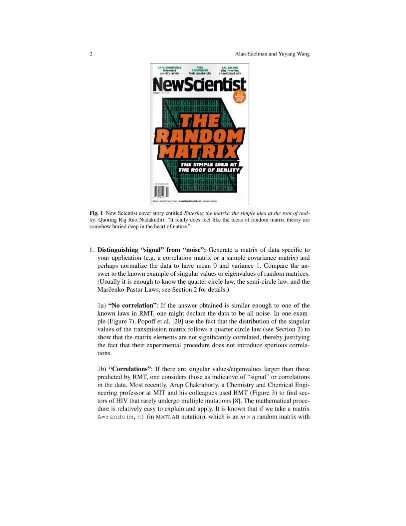
Fig. 1 New Scientist cover story entitled Entering the matrix: the simple idea at the root of real-ity. Quoting Raj Rao Nadakuditi: “It really does feel like the ideas of random matrix theory aresomehow buried deep in the heart of nature.”

1. Distinguishing “signal” from “noise”: Generate a matrix of data specific toyour application (e.g. a correlation matrix or a sample covariance matrix) andperhaps normalize the data to have mean 0 and variance 1. Compare the an-swer to the known example of singular values or eigenvalues of random matrices.(Usually it is enough to know the quarter circle law, the semi-circle law, and theMarcenko-Pastur Laws, see Section 2 for details.)

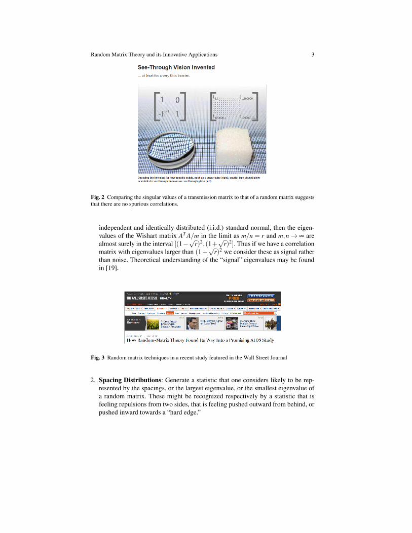
1a) “No correlation”: If the answer obtained is similar enough to one of theknown laws in RMT, one might declare the data to be all noise. In one exam-ple (Figure 7), Popoff et al. [20] use the fact that the distribution of the singularvalues of the transmission matrix follows a quarter circle law (see Section 2) toshow that the matrix elements are not significantly correlated, thereby justifyingthe fact that their experimental procedure does not introduce spurious correla-tions.

1b) “Correlations”: If there are singular values/eigenvalues larger than thosepredicted by RMT, one considers those as indicative of “signal” or correlationsin the data. Most recently, Arup Chakraborty, a Chemistry and Chemical Engi-neering professor at MIT and his colleagues used RMT (Figure 3) to find sec-tors of HIV that rarely undergo multiple mutations [8]. The mathematical proce-dure is relatively easy to explain and apply. It is known that if we take a matrixA=randn(m,n) (in MATLAB notation), which is an m×n random matrix with

Random Matrix Theory and its Innovative Applications 3

Fig. 2 Comparing the singular values of a transmission matrix to that of a random matrix suggeststhat there are no spurious correlations.

independent and identically distributed (i.i.d.) standard normal, then the eigen-values of the Wishart matrix AT A/m in the limit as m/n = r and m,n→ ∞ arealmost surely in the interval [(1−

√r)2,(1+

√r)2]. Thus if we have a correlation

matrix with eigenvalues larger than (1+√

r)2 we consider these as signal ratherthan noise. Theoretical understanding of the “signal” eigenvalues may be foundin [19].

Fig. 3 Random matrix techniques in a recent study featured in the Wall Street Journal

2. Spacing Distributions: Generate a statistic that one considers likely to be rep-resented by the spacings, or the largest eigenvalue, or the smallest eigenvalue ofa random matrix. These might be recognized respectively by a statistic that isfeeling repulsions from two sides, that is feeling pushed outward from behind, orpushed inward towards a “hard edge.”


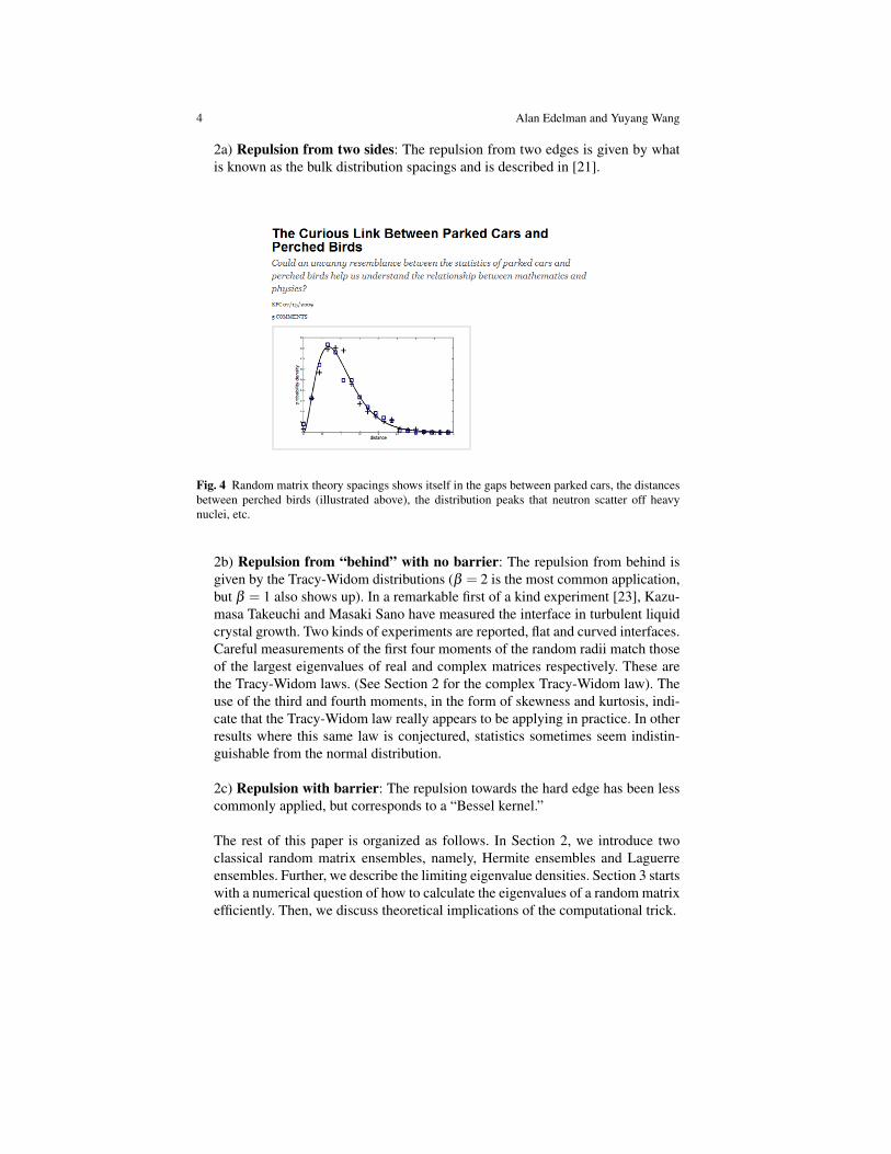
2a) Repulsion from two sides: The repulsion from two edges is given by whatis known as the bulk distribution spacings and is described in [21].

Fig. 4 Random matrix theory spacings shows itself in the gaps between parked cars, the distancesbetween perched birds (illustrated above), the distribution peaks that neutron scatter off heavynuclei, etc.

2b) Repulsion from “behind” with no barrier: The repulsion from behind isgiven by the Tracy-Widom distributions (β = 2 is the most common application,but β = 1 also shows up). In a remarkable first of a kind experiment [23], Kazu-masa Takeuchi and Masaki Sano have measured the interface in turbulent liquidcrystal growth. Two kinds of experiments are reported, flat and curved interfaces.Careful measurements of the first four moments of the random radii match thoseof the largest eigenvalues of real and complex matrices respectively. These arethe Tracy-Widom laws. (See Section 2 for the complex Tracy-Widom law). Theuse of the third and fourth moments, in the form of skewness and kurtosis, indi-cate that the Tracy-Widom law really appears to be applying in practice. In otherresults where this same law is conjectured, statistics sometimes seem indistin-guishable from the normal distribution.

2c) Repulsion with barrier: The repulsion towards the hard edge has been lesscommonly applied, but corresponds to a “Bessel kernel.”

The rest of this paper is organized as follows. In Section 2, we introduce twoclassical random matrix ensembles, namely, Hermite ensembles and Laguerreensembles. Further, we describe the limiting eigenvalue densities. Section 3 startswith a numerical question of how to calculate the eigenvalues of a random matrixefficiently. Then, we discuss theoretical implications of the computational trick.


2 Famous Laws in RMT with MATLAB experiments

We introduce the classic random matrix ensembles and then we will provide fourfamous laws in RMT with corresponding MATLAB experiments. Notice that al-though measure-theoretical probability is not required to understand and appreciatethe beauty of RMT in this paper, the extension of probabilistic measure-theoreticaltools to matrices is nontrivial, we refer interested readers to [6, 2].

While we expect our readers to be familiar with real and complex matrices, it isreasonable to consider quaternion matrices as well. Let us start with the Gaussianrandom matrices G1(m,n) (G1 = randn(m, n)), which is an m×n matrix withi.i.d. standard real random normals. In general, we use the parameter β to denote thenumber of standard real normals and thus β = 1,2,4 correspond to real, complexand quaternion respectively. Gβ (m,n) can be generated by the MATLAB commandshown in Table 1. Notice that since quaternions do not exist in MATLAB they are“faked” using 2×2 complex matrices.

Table 1 Generating the Gaussian random matrix Gβ (m,n) in MATLAB

β MATLAB command1 G = randn(m, n)2 G = randn(m, n) + i*randn(m, n)4 X = randn(m, n) + i*randn(m, n);

Y = randn(m, n) + i*randn(m, n); G = [X Y; -conj(Y) conj(X)]

If A is an m×n Gaussian random matrix Gβ (m,n) then its joint element densityis given by

1

(2π)βmn/2 exp(−1

2‖A‖2

F

), (1)

where ‖ · ‖F is the Frobenius norm of a matrix.The most important property of Gβ , be it real, complex, or quaternion, is its or-

thogonal invariance. This makes the distribution impervious to multiplication byan orthogonal (unitary, symplectic) matrix, provided that the two are independent.This can be inferred from the joint element density in (1) since its Frobenius norm,‖A‖F , is unchanged when A is multiplied by an orthogonal (unitary, symplectic)matrix. The orthogonal invariance implies that no test can be devised that woulddifferentiate between Q1A, A, and AQ2, where Q1 and Q2 are non-random orthog-onal and A is Gaussian. Readers will later see that this simple property leads towonderful results both in practice and in theory.

The most well-studied random matrices have names such as Gaussian, Wishart,MONOVA, and circular. We prefer Hermite, Laguerre, Jacobi, and perhaps Fourier.In a sense, they are to random matrix theory as Poisson’s equation is to numericalmethods. Of course, we are thinking in the sense of the problems that are well-tested,well-analyzed, and well-studied because of nice fundamental analytic properties.


These matrices play a prominent role because of their deep mathematical structure.There are four channels of structure lurking underneath numeric analysis, graphtheory, multivariate statistics [17] and operator algebras [18]. In this paper, we willfocus on the Hermite and Laguerre ensembles, which is summarized in Table 2. Theother random matrix ensembles are discussed in details in [10].

Table 2 Hermite and Laguerre ensembles.

Ensemble Matrices Weight function Equilibrium measure Numeric MATLAB

Hermite Wigner e−x2/2 semi-circle eigg = G(n,n);H=(g+g’)/2

Laguerre Wishart xv/2−1e−x/2 Marcenko-Pastur svdg = G(m,n);L=(g’*g)/m;

2.1 The most famous Semi-circle law

In [24], Wigner originally showed that the limiting eigenvalue distribution of simplerandom symmetric n× n matrices X = (A+AT )/2 where A = G1(n,n), follow asemi-circle distribution, which is given by

p(x) =1

2π

√4− x2. (2)

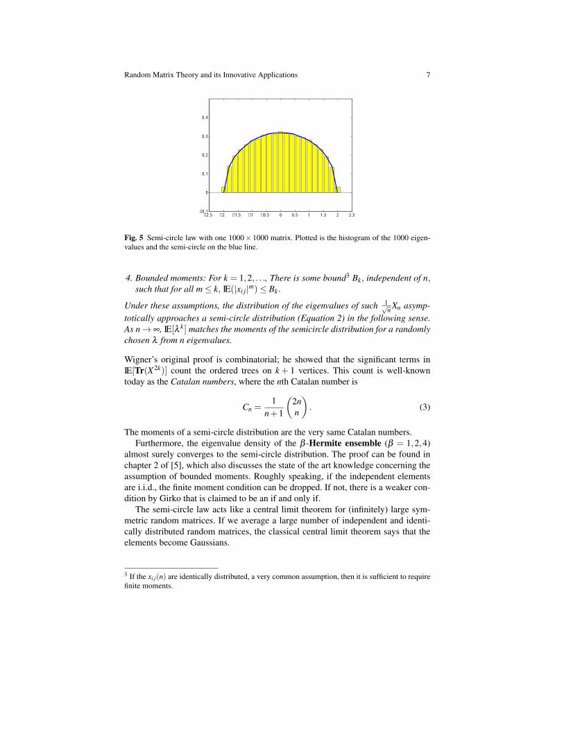
When properly normalized, the curve looks like a semi-circle of radius 2. This dis-tribution depicts the histogram of the n eigenvalues of a symmetric random n× nmatrix obtained by symmetrizing a matrix of random normals. X constructed in thisway is called the β -Hermite ensemble or Gaussian ensemble, more specificallyGaussian orthogonal ensemble (GOE) (β = 1), Gaussian unitary ensemble (GUE)(β = 2) and Gaussian symplectic ensemble (GSE) (β = 4). Code 1 histograms therandom eigenvalues and plots the semi-circle. The mathematical theorem requiresonly one matrix t = 1 and n→∞, though the computer is happier with much smallervalues for n.

Theorem 1. (Wigner 1955) Let Xn be a sequence of random symmetric n×n matri-ces (n = 1,2, . . . .), satisfying

1. Independent elements (up to matrix symmetry): The elements xi j for i≤ j of eachXn are independent random variables2.

2. Zero Mean: The elements xi j of each Xn satisfy IE(xi j) = 0.3. Unit off diagonal variance (for normalization): The elements xi j of each Xn sat-

isfy IE(x2i j) = 1.

2 Strictly speaking, the random variables should be written xi j(n).


−2.5 −2 −1.5 −1 −0.5 0 0.5 1 1.5 2 2.5−0.1

0

0.1

0.2

0.3

0.4

Fig. 5 Semi-circle law with one 1000× 1000 matrix. Plotted is the histogram of the 1000 eigen-values and the semi-circle on the blue line.

4. Bounded moments: For k = 1,2, . . ., There is some bound3 Bk, independent of n,such that for all m≤ k, IE(|xi j|m)≤ Bk.

Under these assumptions, the distribution of the eigenvalues of such 1√n Xn asymp-

totically approaches a semi-circle distribution (Equation 2) in the following sense.As n→∞, IE[λ k] matches the moments of the semicircle distribution for a randomlychosen λ from n eigenvalues.

Wigner’s original proof is combinatorial; he showed that the significant terms inIE[Tr(X2k)] count the ordered trees on k + 1 vertices. This count is well-knowntoday as the Catalan numbers, where the nth Catalan number is

Cn =1

n+1

(2nn

). (3)

The moments of a semi-circle distribution are the very same Catalan numbers.Furthermore, the eigenvalue density of the β -Hermite ensemble (β = 1,2,4)

almost surely converges to the semi-circle distribution. The proof can be found inchapter 2 of [5], which also discusses the state of the art knowledge concerning theassumption of bounded moments. Roughly speaking, if the independent elementsare i.i.d., the finite moment condition can be dropped. If not, there is a weaker con-dition by Girko that is claimed to be an if and only if.

The semi-circle law acts like a central limit theorem for (infinitely) large sym-metric random matrices. If we average a large number of independent and identi-cally distributed random matrices, the classical central limit theorem says that theelements become Gaussians.

3 If the xi j(n) are identically distributed, a very common assumption, then it is sufficient to requirefinite moments.


Another important problem is the convergence rate of the (empirical) eigenvaluedensity, which was answered by Bai in [3, 4]. We refer interested readers to chapter8 of [5].

Code 1 Semicircle Law (Random symmetric matrix eigenvalues)

%E x p e r i m e n t : Gauss ian Random Symmetr i c E i g e n v a l u e s%P l o t : His togram o f t h e e i g e n v a l u e s%Theory : S e m i c i r c l e as n−> i n f i n i t y%% Parame ter sn =1000; %m a t r i x s i z et =1 ; %t r i a l sv = [ ] ; %e i g e n v a l u e samplesdx = . 2 ; %b i n s i z e%% E x p e r i m e n tf o r i =1 : t ,

a=randn ( n ) ; % random nxn m a t r i xs =( a+a ’ ) / 2 ; % s y m m e t r i z e d m a t r i xv =[ v ; e i g ( s ) ] ; % e i g e n v a l u e s

endv=v / s q r t ( n / 2 ) ; % n o r m a l i z e d e i g e n v a l u e s%% P l o t[ count , x ]= h i s t ( v ,−2: dx : 2 ) ;c l a r e s e tbar ( x , c o u n t / ( t ∗n∗dx ) , ’ y ’ ) ;hold on ;%% Theoryp l o t ( x , s q r t (4−x . ˆ 2 ) / ( 2∗ pi ) , ’ LineWidth ’ , 2 )a x i s ( [−2 .5 2 . 5 −.1 . 5 ] ) ;

On the other hand, in the finite case where n is given, one may wonder how arethe eigenvalues of an n× n symmetric random matrix A distributed? Fortunately,for the Hermite ensemble, the answer is known explicitly and the density is calledthe level density in the Physics literature [15]. It is worth mentioning that the jointelement density of an n×n matrix Aβ from the Hermite ensemble is [9]

12n/2

1πn/2+n(n−1)β/4 exp

(−1

2‖A‖2

F

), (4)

and the joint eigenvalue probability density function is

fβ (λ1, · · · ,λn) = cβ

H ∏i< j|λi−λ j|β exp

(−

n

∑i=1

λ 2i

2

), (5)

with

cβ

H = (2π)−n/2n

∏j=1

Γ (1+ β

2 )

Γ (1+ β

2 j).


The level density ρAn for an n×n ensemble A with real eigenvalues is the distribution

of a random eigenvalue chosen from the ensemble. More precisely, the level densitycan be written in terms of the marginalization of the joint eigenvalue density. Forexample, in the Hermite ensemble case,

ρAn,β (λ1) =

∫IRn−1

fβ (λ1, · · · ,λn)dλ2 · · ·dλn. (6)

In the following part, we will show the exact semi-circle for the GUE case and givenumerical approaches that calculate the level density efficiently. Notice that suchformulas also exist for the finite GOE and GSE, we refer interested readers to [15].

If A is a n× n complex Gaussian and we take (A+AT )/2 which is an instanceof the GUE ensemble, the eigenvalue density was derived by Wigner in 1962 as∑

n−1j=0 φ 2

j (x), where

φ j(x) = (2 j j!√

π)−12 exp(−x2/2)H j(x) (7)

and H j(x) is the jth Hermite polynomial, which is defined as

H j(x) = exp(x2)

(− d

dx

) j

exp(−x2) = j!j/2

∑i=0

(−1)i (2x) j−2i

i!( j−2i)!.

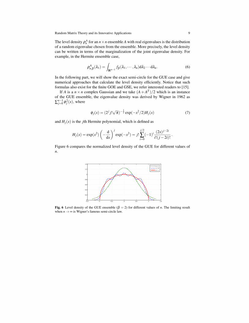
Figure 6 compares the normalized level density of the GUE for different values ofn.

−1.5 −1 −0.5 0 0.5 1 1.50

0.2

0.4

0.6

0.8

1

1.2

1.4

n = 1n = 5

n = ∞

Fig. 6 Level density of the GUE ensemble (β = 2) for different values of n. The limiting resultwhen n→ ∞ is Wigner’s famous semi-circle law.


−1.5 −1 −0.5 0 0.5 1 1.5−1

−0.5

0

0.5

1

1.5

2

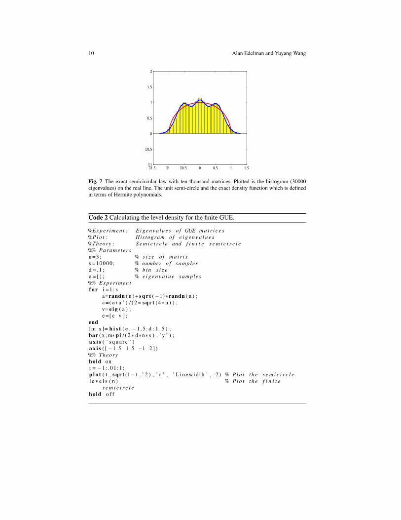
Fig. 7 The exact semicircular law with ten thousand matrices. Plotted is the histogram (30000eigenvalues) on the real line. The unit semi-circle and the exact density function which is definedin terms of Hermite polynomials.

Code 2 Calculating the level density for the finite GUE.

%E x p e r i m e n t : E i g e n v a l u e s o f GUE m a t r i c e s%P l o t : His togram o f e i g e n v a l u e s%Theory : S e m i c i r c l e and f i n i t e s e m i c i r c l e%% Parame ter sn =3; % s i z e o f m a t r i xs =10000; % number o f samplesd = . 1 ; % b i n s i z ee = [ ] ; % e i g e n v a l u e samples%% E x p e r i m e n tf o r i =1 : s

a=randn ( n ) + s q r t (−1)∗randn ( n ) ;a =( a+a ’ ) / ( 2∗ s q r t (4∗ n ) ) ;v= e i g ( a ) ;e =[ e v ] ;

end[m x ]= h i s t ( e , −1 . 5 : d : 1 . 5 ) ;bar ( x ,m∗pi / ( 2∗ d∗n∗ s ) , ’ y ’ ) ;a x i s ( ’ s q u a r e ’ )a x i s ( [−1 .5 1 . 5 −1 2 ] )

%% Theoryhold ont = −1 : . 0 1 : 1 ;p l o t ( t , s q r t (1− t . ˆ 2 ) , ’ r ’ , ’ L i n e w i d t h ’ , 2 ) % P l o t t h e s e m i c i r c l el e v e l s ( n ) % P l o t t h e f i n i t e

s e m i c i r c l ehold o f f


Most useful for computation is the three term recurrence

H j+1(x) = 2xH j(x)−2 jH j−1(x), (8)

starting with H−1 = 0 and H0 = 1 so that H1(x) = 2x. Therefore, ignoring the nor-malization term (

√π)−

12 exp(−x2/2) in φ j(x), we define

φ j(x) = (2 j j!)−12 H j(x).

From Equation 8, we can get the three term recurrence for φ j(x) as follows√j · φ j(x) =

√2x · φ j−1(x)−

√j−1 · φ j−2(x). (9)

Based on Equation 9, one can do the direct calculation of summing φn(x) for eachx. But there are two better ways to calculate the level density.

1. The first approach is based on the following equation

n−1

∑j=0

φ2j (x) = nφ

2n (x)−

√n(n+1)φn−1(x)φn+1(x). (10)

This formula comes from the famous Christoffel-Darboux relationship for or-thogonal polynomials. Therefore, we can combine Equation 10 with the threeterm recurrence for φ and Code 3 realizes the idea.

Code 3 Computing the level density (GUE) using Christoffel-Darboux.

f u n c t i o n z= l e v e l s ( n )%P l o t e x a c t s e m i c i r c l e f o r m u l a f o r GUEx = [ −1 : . 0 0 1 : 1 ]∗ s q r t (2∗ n ) ∗ 1 . 3 ;po ld = 0∗x ; % −1 s t Hermi te p o l y n o m i a lp= 1+0∗x ; % 0 t h Hermi te p o l y n o m i a lk=p ;f o r j =1 : n ; % Three term r e c u r r e n c e

pnew = ( s q r t ( 2 ) ∗x .∗ p−s q r t ( j −1)∗ po ld ) / s q r t ( j ) ;po ld = p ; p=pnew ;

endpnew = ( s q r t ( 2 ) ∗x .∗ p−s q r t ( n ) ∗ po ld ) / s q r t ( n +1) ;k = n∗p .ˆ2− s q r t ( n ∗ ( n +1) ) ∗pnew .∗ po ld ; % Use p . 4 2 0 o f Mehta% M u l t i p l y t h e c o r r e c t n o r m a l i z a t i o nk=k .∗ exp(−x . ˆ 2 ) / s q r t ( pi ) ;% R e s c a l e so t h a t ” s e m i c i r c l e ” i s on [−1 ,1] and area i s p i / 2p l o t ( x / s q r t (2∗ n ) , k∗pi / s q r t (2∗ n ) , ’ b ’ , ’ L i n e w i d t h ’ , 2 ) ;

2. The other way comes from the following interesting equivalent expression


n−1

∑j=0

φ2j (x) = ‖(

√π)−

12 exp(−x2/2) · v‖2, (11)

wherev =

uu1

, u = (T −√

2x · I)−1en−1. (12)

where u1 is the first element of u and en−1 is the column vector where onlythe n− 1st entry is 1. T is a tridiagonal matrix that is related to the three termrecurrence such that

T =

0√

1 0 0 · · · 0√1 0

√2 0 · · · 0

0√

2 0√

3 0 · · ·...

......

......

...0 0 0 · · ·

√n−1 0

.

To see this, from Equation 9, we have the following relation−√

2x√

1 0 · · · 0√1 −

√2x√

2 · · · 00

√2 −

√2x

√3 · · ·

......

......

...0 0 · · ·

√n−1 −

√2x

φ0(x)φ1(x)φ2(x)

...φn−1(x)

=C×

000...1

,

where C can be determined easily by the initial condition φ0(x) = 1 which justi-fies Equation 12.Though one can easily use Equation 11 to compute the density at x, we can avoidinverting T −

√2x · I for every x. Given the eigendecomposition of T = HΛHT ,

we have

u = (T −√

2x · I)−1en−1

= H(Λ −√

2x · I)−1HT en−1.

Thus, for each x, we only need to invert the diagonal matrix Λ−√

2x ·I, providedthat H is stored beforehand. Code 4 gives the corresponding implementation.


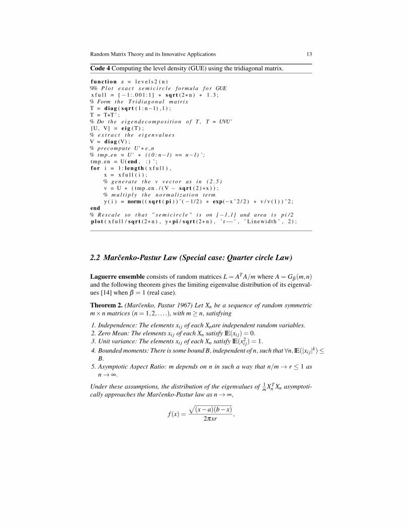
Code 4 Computing the level density (GUE) using the tridiagonal matrix.

f u n c t i o n z = l e v e l s 2 ( n )%% P l o t e x a c t s e m i c i r c l e f o r m u l a f o r GUEx f u l l = [ −1 : . 0 0 1 : 1 ] ∗ s q r t (2∗ n ) ∗ 1 . 3 ;

% Form t h e T r i d i a g o n a l m a t r i xT = diag ( s q r t ( 1 : n−1) , 1 ) ;T = T+T ’ ;% Do t h e e i g e n d e c o m p o s i t i o n o f T , T = UVU’[U, V] = e i g ( T ) ;% e x t r a c t t h e e i g e n v a l u e sV = diag (V) ;% precompute U’∗ e n% tmp en = U’ ∗ ( ( 0 : n−1) == n−1) ’ ;tmp en = U( end , : ) ’ ;f o r i = 1 : l e n g t h ( x f u l l ) ,

x = x f u l l ( i ) ;% g e n e r a t e t h e v v e c t o r as i n ( 2 . 5 )v = U ∗ ( tmp en . / ( V − s q r t ( 2 ) ∗x ) ) ;% m u l t i p l y t h e n o r m a l i z a t i o n termy ( i ) = norm ( ( s q r t ( pi ) ) ˆ ( −1 / 2 ) ∗ exp(−x ˆ 2 / 2 ) ∗ v / v ( 1 ) ) ˆ 2 ;

end% R e s c a l e so t h a t ” s e m i c i r c l e ” i s on [−1 ,1] and area i s p i / 2p l o t ( x f u l l / s q r t (2∗ n ) , y∗pi / s q r t (2∗ n ) , ’ r−−’ , ’ L i n e w i d t h ’ , 2 ) ;

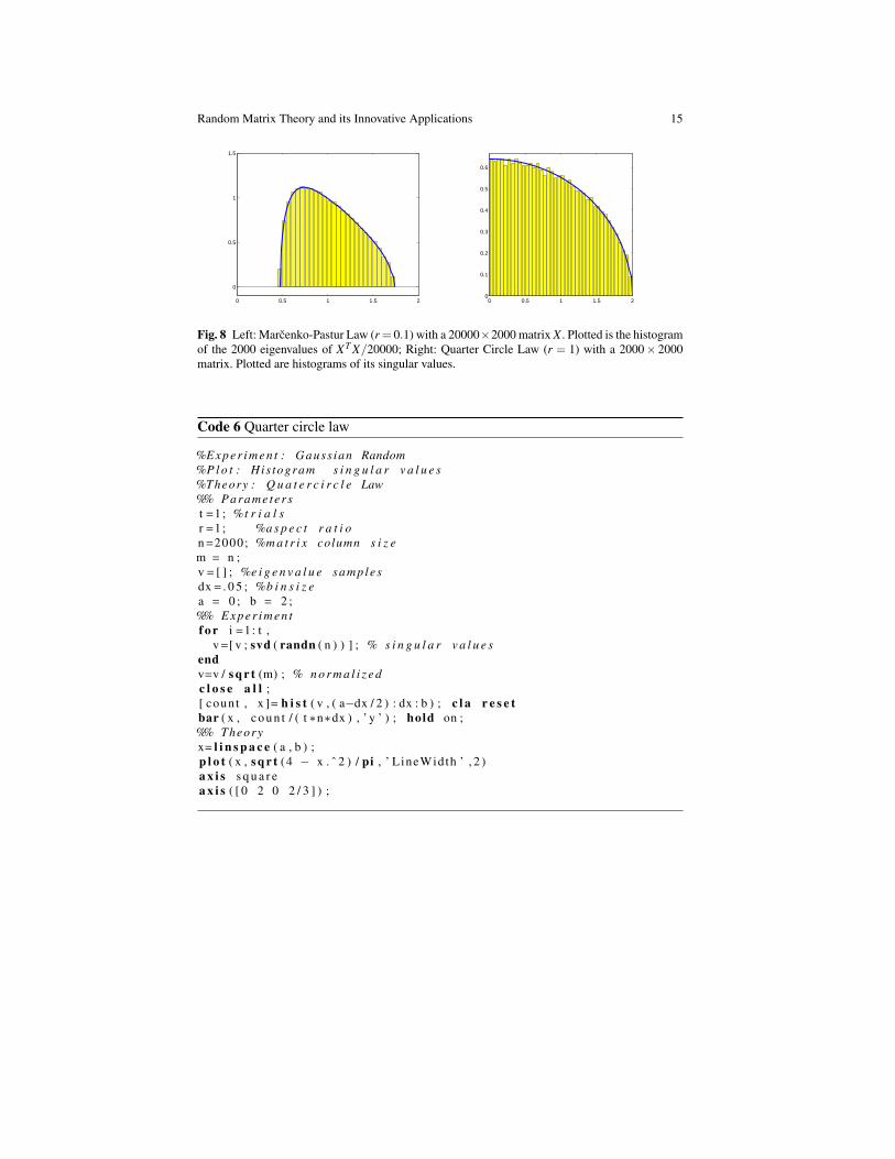
2.2 Marcenko-Pastur Law (Special case: Quarter circle Law)

Laguerre ensemble consists of random matrices L = AT A/m where A = Gβ (m,n)and the following theorem gives the limiting eigenvalue distribution of its eigenval-ues [14] when β = 1 (real case).

Theorem 2. (Marcenko, Pastur 1967) Let Xn be a sequence of random symmetricm×n matrices (n = 1,2, . . . .), with m≥ n, satisfying

1. Independence: The elements xi j of each Xnare independent random variables.2. Zero Mean: The elements xi j of each Xn satisfy IE(xi j) = 0.3. Unit variance: The elements xi j of each Xn satisfy IE(x2

i j) = 1.4. Bounded moments: There is some bound B, independent of n, such that ∀n, IE(|xi j|k)≤

B.5. Asymptotic Aspect Ratio: m depends on n in such a way that n/m→ r ≤ 1 as

n→ ∞.

Under these assumptions, the distribution of the eigenvalues of 1m XT

n Xn asymptoti-cally approaches the Marcenko-Pastur law as n→ ∞,

f (x) =

√(x−a)(b− x)

2πxr,


where a = (1−√

r)2 and b = (1+√

r)2.

Code 5 Marcenko-Pastur Law

%E x p e r i m e n t : Gauss ian Random%P l o t : His togram o f t h e e i g e n v a l u e s o f X ’ X /m%Theory : Marcenko−P a s t u r as n−> i n f i n i t y%% Parame ter st =1 ; %t r i a l sr = 0 . 1 ; %a s p e c t r a t i on =2000; %m a t r i x column s i z em=round ( n / r ) ;v = [ ] ; %e i g e n v a l u e samplesdx = . 0 5 ; %b i n s i z e%% E x p e r i m e n tf o r i =1 : t ,

X=randn (m, n ) ; % random mxn m a t r i xs=X’∗X; %sym pos d e f m a t r i xv =[ v ; e i g ( s ) ] ; % e i g e n v a l u e s

endv=v /m; % n o r m a l i z e d e i g e n v a l u e sa=(1− s q r t ( r ) ) ˆ 2 ; b =(1+ s q r t ( r ) ) ˆ 2 ;%% P l o t[ count , x ]= h i s t ( v , a : dx : b ) ;c l a r e s e tbar ( x , c o u n t / ( t ∗n∗dx ) , ’ y ’ ) ;hold on ;%% Theoryx= l i n s p a c e ( a , b ) ;p l o t ( x , s q r t ( ( x−a ) . ∗ ( b−x ) ) . / ( 2 ∗ pi∗x∗ r ) , ’ LineWidth ’ , 2 )a x i s ( [ 0 c e i l ( b ) −.1 1 . 5 ] ) ;

According to the Marcenko-Pastur Law, we have the density of the singular val-ues of X/

√m as

f (s) =

√(s2−a2)(b2− s2)

πsr.

When r = 1, we get the special case that

f (s) =1π

√4− s2,

on [0,2]. This is the famous quarter circle law. The singular values of a normallydistributed square matrix lie on a quarter circle. The moments are Catalan numbers.We provide the code of the eigenvalue formulations in Code 5 and the singular valueformulation in Code 6 with figures shown in Figure 8.


0 0.5 1 1.5 2

0

0.5

1

1.5

0 0.5 1 1.5 20

0.1

0.2

0.3

0.4

0.5

0.6

Fig. 8 Left: Marcenko-Pastur Law (r = 0.1) with a 20000×2000 matrix X . Plotted is the histogramof the 2000 eigenvalues of XT X/20000; Right: Quarter Circle Law (r = 1) with a 2000× 2000matrix. Plotted are histograms of its singular values.

Code 6 Quarter circle law

%E x p e r i m e n t : Gauss ian Random%P l o t : His togram s i n g u l a r v a l u e s%Theory : Q u a t e r c i r c l e Law%% Parame ter st =1 ; %t r i a l sr =1 ; %a s p e c t r a t i on =2000; %m a t r i x column s i z em = n ;v = [ ] ; %e i g e n v a l u e samplesdx = . 0 5 ; %b i n s i z ea = 0 ; b = 2 ;%% E x p e r i m e n tf o r i =1 : t ,

v =[ v ; svd ( randn ( n ) ) ] ; % s i n g u l a r v a l u e sendv=v / s q r t (m) ; % n o r m a l i z e dc l o s e a l l ;[ count , x ]= h i s t ( v , ( a−dx / 2 ) : dx : b ) ; c l a r e s e tbar ( x , c o u n t / ( t ∗n∗dx ) , ’ y ’ ) ; hold on ;%% Theoryx= l i n s p a c e ( a , b ) ;p l o t ( x , s q r t (4 − x . ˆ 2 ) / pi , ’ LineWidth ’ , 2 )a x i s s q u a r ea x i s ( [ 0 2 0 2 / 3 ] ) ;


−1.5 −1 −0.5 0 0.5 1 1.5−1.5

−1

−0.5

0

0.5

1

1.5

−1.5 −1 −0.5 0 0.5 1 1.5−1.5

−1

−0.5

0

0.5

1

1.5

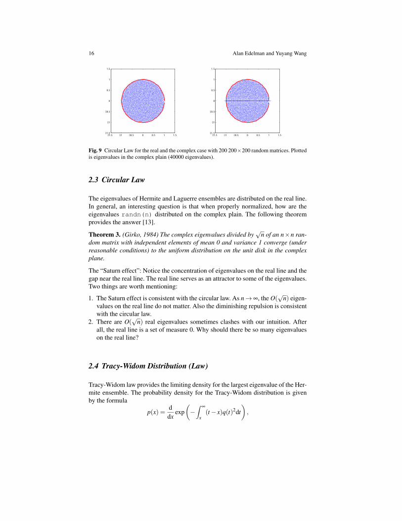
Fig. 9 Circular Law for the real and the complex case with 200 200×200 random matrices. Plottedis eigenvalues in the complex plain (40000 eigenvalues).

2.3 Circular Law

The eigenvalues of Hermite and Laguerre ensembles are distributed on the real line.In general, an interesting question is that when properly normalized, how are theeigenvalues randn(n) distributed on the complex plain. The following theoremprovides the answer [13].

Theorem 3. (Girko, 1984) The complex eigenvalues divided by√

n of an n×n ran-dom matrix with independent elements of mean 0 and variance 1 converge (underreasonable conditions) to the uniform distribution on the unit disk in the complexplane.

The “Saturn effect”: Notice the concentration of eigenvalues on the real line and thegap near the real line. The real line serves as an attractor to some of the eigenvalues.Two things are worth mentioning:

1. The Saturn effect is consistent with the circular law. As n→∞, the O(√

n) eigen-values on the real line do not matter. Also the diminishing repulsion is consistentwith the circular law.

2. There are O(√

n) real eigenvalues sometimes clashes with our intuition. Afterall, the real line is a set of measure 0. Why should there be so many eigenvalueson the real line?

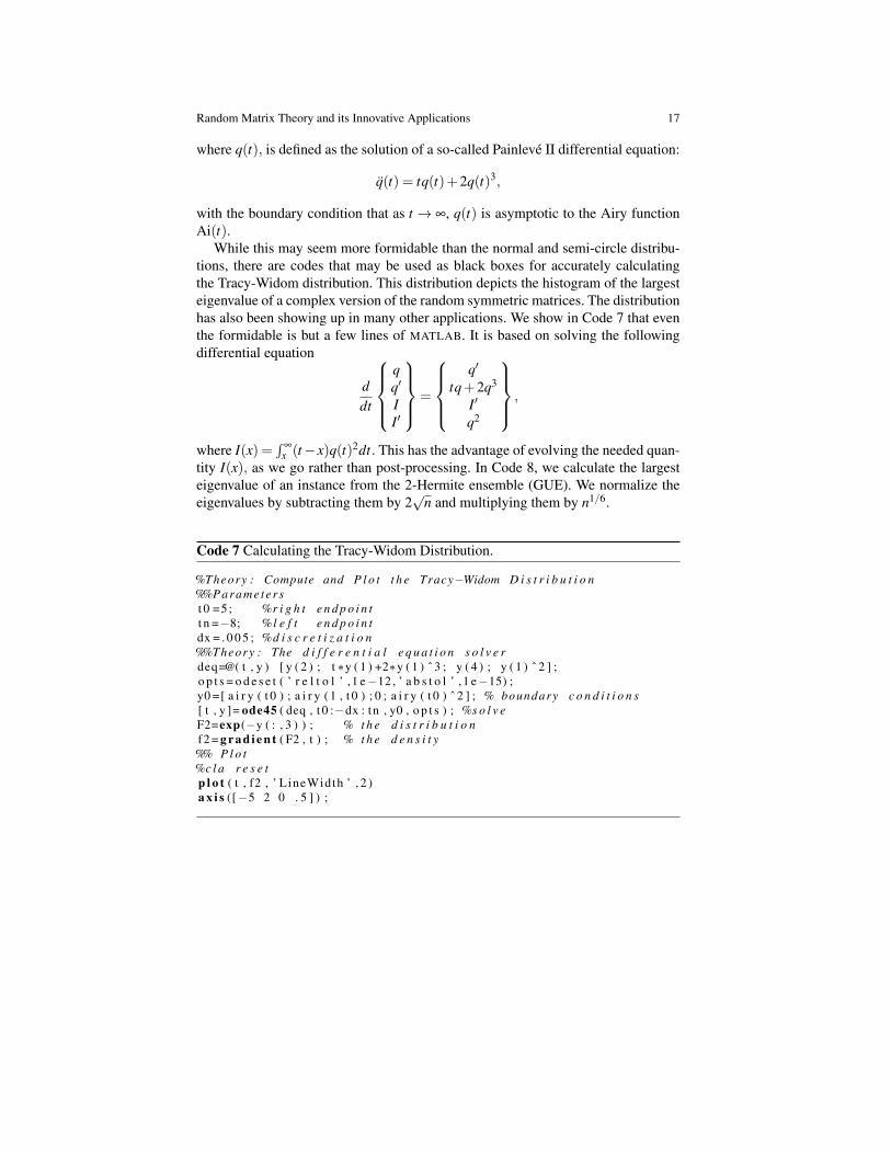
2.4 Tracy-Widom Distribution (Law)

Tracy-Widom law provides the limiting density for the largest eigenvalue of the Her-mite ensemble. The probability density for the Tracy-Widom distribution is givenby the formula

p(x) =ddx

exp(−∫

∞

x(t− x)q(t)2dt

),


where q(t), is defined as the solution of a so-called Painleve II differential equation:

q(t) = tq(t)+2q(t)3,

with the boundary condition that as t → ∞, q(t) is asymptotic to the Airy functionAi(t).

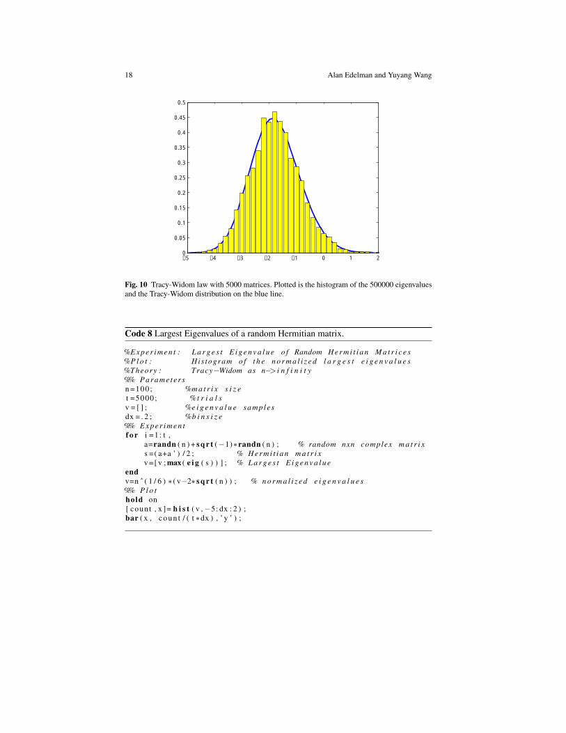
While this may seem more formidable than the normal and semi-circle distribu-tions, there are codes that may be used as black boxes for accurately calculatingthe Tracy-Widom distribution. This distribution depicts the histogram of the largesteigenvalue of a complex version of the random symmetric matrices. The distributionhas also been showing up in many other applications. We show in Code 7 that eventhe formidable is but a few lines of MATLAB. It is based on solving the followingdifferential equation

ddt

qq′

II′

=

q′

tq+2q3

I′

q2

,

where I(x) =∫

∞

x (t−x)q(t)2dt. This has the advantage of evolving the needed quan-tity I(x), as we go rather than post-processing. In Code 8, we calculate the largesteigenvalue of an instance from the 2-Hermite ensemble (GUE). We normalize theeigenvalues by subtracting them by 2

√n and multiplying them by n1/6.

Code 7 Calculating the Tracy-Widom Distribution.

%Theory : Compute and P l o t t h e Tracy−Widom D i s t r i b u t i o n%%Parame ter st 0 =5 ; %r i g h t e n d p o i n tt n =−8; %l e f t e n d p o i n tdx = . 0 0 5 ; %d i s c r e t i z a t i o n%%Theory : The d i f f e r e n t i a l e q u a t i o n s o l v e rdeq=@( t , y ) [ y ( 2 ) ; t ∗y ( 1 ) +2∗y ( 1 ) ˆ 3 ; y ( 4 ) ; y ( 1 ) ˆ 2 ] ;o p t s = o d e s e t ( ’ r e l t o l ’ ,1 e−12 , ’ a b s t o l ’ ,1 e−15) ;y0 =[ a i r y ( t 0 ) ; a i r y ( 1 , t 0 ) ; 0 ; a i r y ( t 0 ) ˆ 2 ] ; % boundary c o n d i t i o n s[ t , y ]= ode45 ( deq , t 0 :−dx : tn , y0 , o p t s ) ; %s o l v eF2=exp(−y ( : , 3 ) ) ; % t h e d i s t r i b u t i o nf2 = g r a d i e n t ( F2 , t ) ; % t h e d e n s i t y%% P l o t%c l a r e s e tp l o t ( t , f2 , ’ LineWidth ’ , 2 )a x i s ([−5 2 0 . 5 ] ) ;


−5 −4 −3 −2 −1 0 1 20

0.05

0.1

0.15

0.2

0.25

0.3

0.35

0.4

0.45

0.5

Fig. 10 Tracy-Widom law with 5000 matrices. Plotted is the histogram of the 500000 eigenvaluesand the Tracy-Widom distribution on the blue line.

Code 8 Largest Eigenvalues of a random Hermitian matrix.

%E x p e r i m e n t : L a r g e s t E i g e n v a l u e o f Random H e r m i t i a n M a t r i c e s%P l o t : His togram o f t h e n o r m a l i z e d l a r g e s t e i g e n v a l u e s%Theory : Tracy−Widom as n−> i n f i n i t y%% Parame ter sn =100; %m a t r i x s i z et =5000; %t r i a l sv = [ ] ; %e i g e n v a l u e samplesdx = . 2 ; %b i n s i z e%% E x p e r i m e n tf o r i =1 : t ,

a=randn ( n ) + s q r t (−1)∗randn ( n ) ; % random nxn complex m a t r i xs =( a+a ’ ) / 2 ; % H e r m i t i a n m a t r i xv =[ v ; max ( e i g ( s ) ) ] ; % L a r g e s t E i g e n v a l u e

endv=n ˆ ( 1 / 6 ) ∗ ( v−2∗ s q r t ( n ) ) ; % n o r m a l i z e d e i g e n v a l u e s%% P l o thold on[ count , x ]= h i s t ( v ,−5: dx : 2 ) ;bar ( x , c o u n t / ( t ∗dx ) , ’ y ’ ) ;


3 Random Matrix Factorization

A computational trick can also be a theoretical trick. Therefore do not dismiss anefficient computation as a mere “implementation detail”, it may be where the nexttheory comes from.

Direct random matrix experiments usually involve randn(n). Since many lin-ear algebra computations require O(n3) operations, it seems more feasible to take nrelatively small, and take a large number of Monte Carlo instances. This has beenour strategy in the example codes so far.

In fact, matrix computations involve a series of reductions. With normally dis-tributed matrices, the most expensive reduction steps can be avoided on the com-puter as they can be done with mathematics! All of a sudden O(n3) computationsbecome O(n2) or even better.

3.1 The Chi-distribution and orthogonal invariance

There are two key facts to know about a vector of independent standard normals. Letvn denote such a vector. In MATLAB this would be randn(n,1). Mathematically,we say that the n elements are independent and i.i.d. standard normals (mean 0,variance 1).

• Chi distribution: the Euclidean length ‖vn‖, which is the square root of the sumof the n squares of Gaussians, has what is known as the χn distribution.

• Orthogonal Invariance: for any fixed orthogonal matrix Q, or if Q is randomand independent of vn, the distribution of Qvn is identical to that of vn. In otherwords, it is impossible to tell the difference between a computer-generated vn orQvn upon inspecting only the output.

We shall see that these two facts allow us to very powerfully transform matricesinvolving standard normals to simpler forms. For reference, we mention that the χndistribution has the probability density

f (x) =xn−1e−x2/2

2n/2−1Γ (n/2). (13)

There is no specific requirement that n be an integer, despite our original motivationas the length of a Gaussian vector. The square of χn is the distribution that underliesthe well known Chi-squared test. It can be seen that the mean of χ2

n is n. (Forintegers, it is the sum of the n standard normal variables). We have that vn is theproduct of the random scalar χn, which serves as the length, and an independentvector that is uniform on the sphere, which serves as the direction.


3.2 The QR decomposition of randn(n)

Given a vector vn, we can readily construct an orthogonal reflection or rotation Hnsuch that Hnvn = ±‖vn‖e1, where e1 denotes the first column of the identity. Inmatrix computations, there is a standard technique known as constructing a House-holder transformation which is a reflection across the external angle bisector ofthese two vectors.

Therefore, if vn follows a multivariate standard normal distribution, Hnvn yieldsa Chi distribution for the first element and 0 otherwise. Furthermore, let randn(n)be an n× n matrix of iid standard normals. It is easy to see now that through suc-cessive Householder reflections of size n,n− 1, . . . we can orthogonally transformrandn(n) into the upper triangular matrix

H1H2 · · ·Hn−1Hn×randn(n)= Rn =

χn G G . . . G G Gχn−1 G . . . G G G

χn−2 . . . G G G. . .

......

...χ3 G G

χ2 Gχ1

.

Here all elements are independent and represent a distribution and the “G”’ are alli.i.d. standard normals. It is helpful to watch a 3× 3 real Gaussian matrix (β = 1)matrix turn into R:G G G

G G GG G G

→ χ3 G G

0 G G0 G G

→ χ3 G G

0 χ2 G0 0 G

→ χ3 G G

0 χ2 G0 0 χ1

.

The “G”’s as the computation progresses are not the same numbers, merely indicat-ing the distribution. One immediate consequence is the following interesting fact

IE[det(randn(n)2)] = n! (14)

This could also be obtained for any n×n matrix with independent entries with mean0 and variance 1, by squaring the “big formula” for the determinant, noting that crossterms have expectation 0, and the n! squared terms each have expectation 1.

3.2.1 Haar measure on Orthogonal matrices

Let Q be a random orthogonal matrix, such that one can not tell the difference be-tween the distribution of AQ and Q for any fixed orthogonal matrix A. We say thatQ has the uniform or Haar distribution on orthogonal matrices.


From the previous part of this section, with a bit of care we can say thatrandn(n)=(orthogonal uniform with Haar measure)(Rn) is the QR decompositionof randn(n). Therefore, code for generating Q can be as simple as [Q,∼]=qr(randn(n)).

Similarly, [Q,∼]=qr(randn(n)+sqrt(-1)*randn(n)) gives a randomunitary matrix Q. For unitary matrix Q, its eigenvalues will be complex with a mag-nitude of 1, i.e. they will be distributed on the unit circle in the complex plane.Code 9 generates a random unitary matrix and histograms the angles of its eigen-values.

Code 9 Sample a random unitary matrix.

%E x p e r i m e n t : Genera te random o r t h o g o n a l / u n i t a r y m a t r i c e s%P l o t : His togram e i g e n v a l u e s%Theory : E i g e n v a l u e s are on u n i t c i r c l e%% Parame ter st =5000; %t r i a l sdx = . 0 5 ; %b i n s i z en =10; %m a t r i x s i z ev = [ ] ; %e i g e n v a l u e samples%% E x p e r i m e n tf o r i =1 : t

% Sample random u n i t a r y m a t r i x[X ˜ ] = qr ( randn ( n ) + s q r t (−1)∗randn ( n ) ) ;% I f you have non−u n i f o r m l y sampled e i g e n v a l u e s , you may

need t h i s f i xX=X∗diag ( s i g n ( randn ( n , 1 ) + s q r t (−1)∗randn ( n , 1 ) ) ) ;v =[ v ; e i g (X) ] ;

end%% P l o tx=(−(1+ dx / 2 ) : dx : ( 1 + dx / 2 ) ) ∗pi ;h1= rose ( ang le ( v ) , x ) ;s e t ( h1 , ’ Co lo r ’ , ’ b l a c k ’ )

%% Theoryhold onh2= po lar ( x , t ∗n∗dx /2∗ x . ˆ 0 ) ;s e t ( h2 , ’ LineWidth ’ , 2 )hold o f f

3.2.2 Longest increasing subsequence

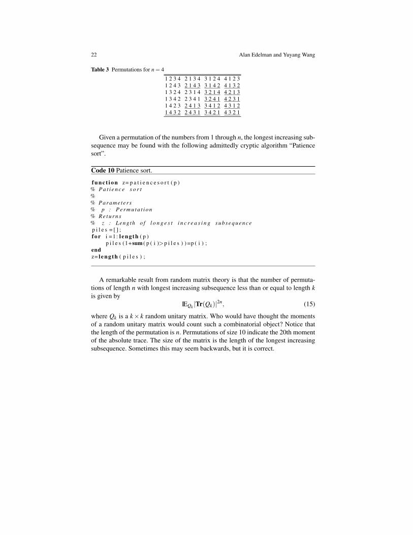
There is an interesting link between the moments of the eigenvalues of Q and thenumber of permutations of length with longest increasing subsequence k. For exam-ple, the permutation ( 3 1 8 4 5 7 2 6 9 10 ) has ( 1 4 5 7 9 10 ) or ( 1 4 5 6 9 10 )as the longest increasing subsequence of length 6. For n = 4, there are 24 possiblepermutations listed in Table 3. We underline the fourteen permutations with longestincreasing subsequence of length 2. Of these, one permutation ( 4 3 2 1) has length1 and the other thirteen have length 2.


Table 3 Permutations for n = 4

1 2 3 4 2 1 3 4 3 1 2 4 4 1 2 31 2 4 3 2 1 4 3 3 1 4 2 4 1 3 21 3 2 4 2 3 1 4 3 2 1 4 4 2 1 31 3 4 2 2 3 4 1 3 2 4 1 4 2 3 11 4 2 3 2 4 1 3 3 4 1 2 4 3 1 21 4 3 2 2 4 3 1 3 4 2 1 4 3 2 1

Given a permutation of the numbers from 1 through n, the longest increasing sub-sequence may be found with the following admittedly cryptic algorithm “Patiencesort”.

Code 10 Patience sort.

f u n c t i o n z= p a t i e n c e s o r t ( p )% P a t i e n c e s o r t%% Parame ter s% p : P e r m u t a t i o n% R e t u r n s% z : Leng th o f l o n g e s t i n c r e a s i n g s u b s e q u e n c ep i l e s = [ ] ;f o r i =1 : l e n g t h ( p )

p i l e s (1+sum ( p ( i )>p i l e s ) ) =p ( i ) ;endz= l e n g t h ( p i l e s ) ;

A remarkable result from random matrix theory is that the number of permuta-tions of length n with longest increasing subsequence less than or equal to length kis given by

IEQk |Tr(Qk)|2n, (15)

where Qk is a k× k random unitary matrix. Who would have thought the momentsof a random unitary matrix would count such a combinatorial object? Notice thatthe length of the permutation is n. Permutations of size 10 indicate the 20th momentof the absolute trace. The size of the matrix is the length of the longest increasingsubsequence. Sometimes this may seem backwards, but it is correct.


Code 11 Random Orthogonal matrices and the Longest increasing sequence.

%E x p e r i m e n t : Counts l o n g e s t i n c r e a s i n g s u b s e q u e n c e s t a t i s t i c st =200000; % Number o f t r i a l sn =4; % p e r m u t a t i o n s i z ek =2; % l e n g t h o f l o n g e s t i n c r e a s i n g s u b s e q u e n c ev= z e r o s ( t , 1 ) ; % samplesf o r i =1 : t

[X,DC]= qr ( randn ( k ) + s q r t (−1)∗randn ( k ) ) ;X=X∗diag ( s i g n ( randn ( k , 1 ) + s q r t (−1)∗randn ( k , 1 ) ) ) ;v ( i ) =abs ( t r a c e (X) ) ˆ ( 2∗ n ) ;

endz = mean ( v ) ;p = perms ( 1 : n ) ; c = 0 ;f o r i =1 : f a c t o r i a l ( n )

c = c + ( p a t i e n c e s o r t ( p ( i , : ) ) <= k ) ;end[ z c ]

3.3 The tridiagonal reductions of GOE

Eigenvalues are usually defined early in one’s education as the roots of the charac-teristic polynomial. Many people just assume that this is the definition that is usedduring a computation, but it is well established that this is not a good method forcomputing eigenvalues. Rather, a matrix factorization is used. In the case that S issymmetric, an orthogonal matrix Q is found such that QT SQ = Λ is diagonal. Thecolumns of Q are the eigenvectors and the diagonal of Λ are the eigenvalues.

Mathematically, the construction of Q is an iterative procedure, requiring in-finitely many steps to converge. In practice, S is first tridiagonalized through a finiteprocess which usually takes the bulk of the time. The tridiagonal is then iterativelydiagonalized. Usually, this takes a negligible amount of time to converge in finiteprecision.

If X = randn(n) and S = (X +XT )/√

2, then the eigenvalues of S follow thesemi-circle law while the largest one follows the Tracy-Widom law. We can tridiag-onalize S with the finite Householder procedure. The result is

Tn =

G√

2 χn−1

χn−1 G√

2 χn−2

χn−2 G√

2 χn−3

χn−3 . . . . . .. . . G

√2 χ2

χ2 G√

2 χ1

χ1 G√

2

, (16)


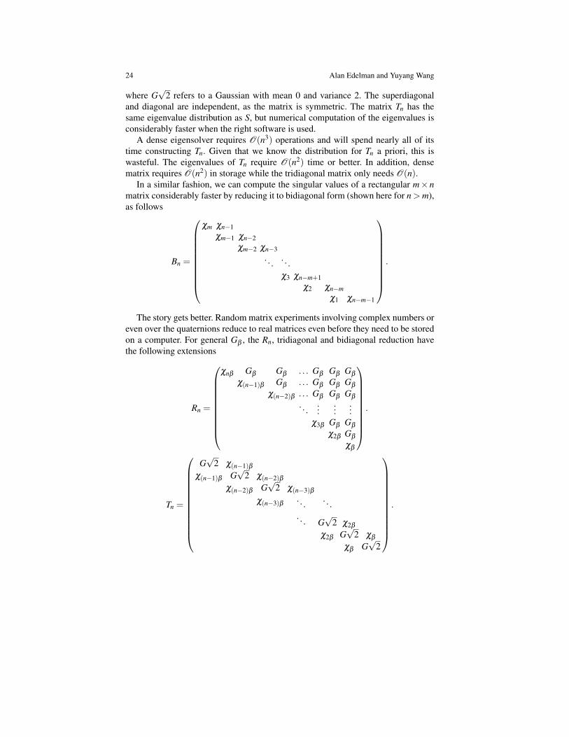
where G√

2 refers to a Gaussian with mean 0 and variance 2. The superdiagonaland diagonal are independent, as the matrix is symmetric. The matrix Tn has thesame eigenvalue distribution as S, but numerical computation of the eigenvalues isconsiderably faster when the right software is used.

A dense eigensolver requires O(n3) operations and will spend nearly all of itstime constructing Tn. Given that we know the distribution for Tn a priori, this iswasteful. The eigenvalues of Tn require O(n2) time or better. In addition, densematrix requires O(n2) in storage while the tridiagonal matrix only needs O(n).

In a similar fashion, we can compute the singular values of a rectangular m× nmatrix considerably faster by reducing it to bidiagonal form (shown here for n > m),as follows

Bn =

χm χn−1χm−1 χn−2

χm−2 χn−3. . . . . .

χ3 χn−m+1χ2 χn−m

χ1 χn−m−1

.

The story gets better. Random matrix experiments involving complex numbers oreven over the quaternions reduce to real matrices even before they need to be storedon a computer. For general Gβ , the Rn, tridiagonal and bidiagonal reduction havethe following extensions

Rn =

χnβ Gβ Gβ . . . Gβ Gβ Gβ

χ(n−1)β Gβ . . . Gβ Gβ Gβ

χ(n−2)β . . . Gβ Gβ Gβ

. . ....

......

χ3β Gβ Gβ

χ2β Gβ

χβ

.

Tn =

G√

2 χ(n−1)βχ(n−1)β G

√2 χ(n−2)β

χ(n−2)β G√

2 χ(n−3)β

χ(n−3)β . . . . . .. . . G

√2 χ2β

χ2β G√

2 χβ

χβ G√

2

.


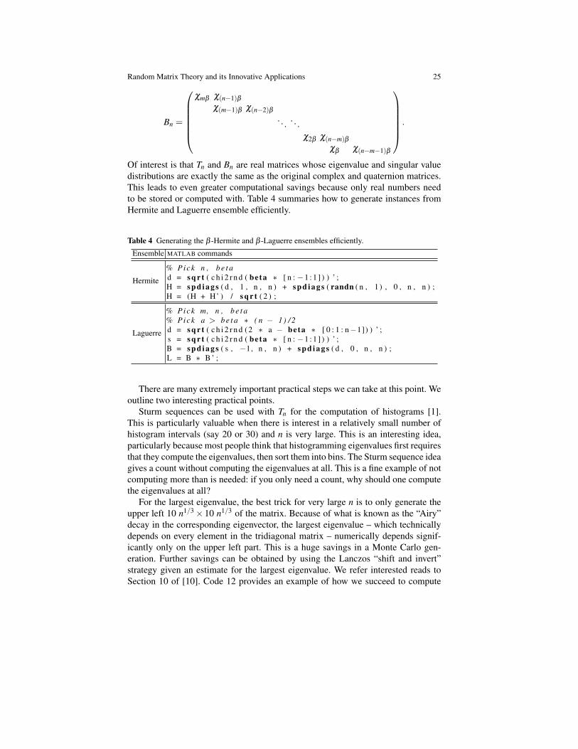
Bn =

χmβ χ(n−1)β

χ(m−1)β χ(n−2)β. . . . . .

χ2β χ(n−m)β

χβ χ(n−m−1)β

.

Of interest is that Tn and Bn are real matrices whose eigenvalue and singular valuedistributions are exactly the same as the original complex and quaternion matrices.This leads to even greater computational savings because only real numbers needto be stored or computed with. Table 4 summaries how to generate instances fromHermite and Laguerre ensemble efficiently.

Table 4 Generating the β -Hermite and β -Laguerre ensembles efficiently.

Ensemble MATLAB commands

Hermite

% Pick n , b e t ad = s q r t ( c h i 2 r n d ( beta ∗ [ n : −1 : 1 ] ) ) ’ ;H = s p d i a g s ( d , 1 , n , n ) + s p d i a g s ( randn ( n , 1 ) , 0 , n , n ) ;H = (H + H’ ) / s q r t ( 2 ) ;

Laguerre

% Pick m, n , b e t a% Pick a > b e t a ∗ ( n − 1) / 2d = s q r t ( c h i 2 r n d (2 ∗ a − beta ∗ [ 0 : 1 : n−1]) ) ’ ;s = s q r t ( c h i 2 r n d ( beta ∗ [ n : −1 : 1 ] ) ) ’ ;B = s p d i a g s ( s , −1, n , n ) + s p d i a g s ( d , 0 , n , n ) ;L = B ∗ B ’ ;

There are many extremely important practical steps we can take at this point. Weoutline two interesting practical points.

Sturm sequences can be used with Tn for the computation of histograms [1].This is particularly valuable when there is interest in a relatively small number ofhistogram intervals (say 20 or 30) and n is very large. This is an interesting idea,particularly because most people think that histogramming eigenvalues first requiresthat they compute the eigenvalues, then sort them into bins. The Sturm sequence ideagives a count without computing the eigenvalues at all. This is a fine example of notcomputing more than is needed: if you only need a count, why should one computethe eigenvalues at all?

For the largest eigenvalue, the best trick for very large n is to only generate theupper left 10 n1/3×10 n1/3 of the matrix. Because of what is known as the “Airy”decay in the corresponding eigenvector, the largest eigenvalue – which technicallydepends on every element in the tridiagonal matrix – numerically depends signif-icantly only on the upper left part. This is a huge savings in a Monte Carlo gen-eration. Further savings can be obtained by using the Lanczos “shift and invert”strategy given an estimate for the largest eigenvalue. We refer interested reads toSection 10 of [10]. Code 12 provides an example of how we succeed to compute


the largest eigenvalue of a billion by billion matrix in the time required by naivemethods for a hundred by hundred matrix.

Code 12 Compute the largest eigenvalues of a billion by billion matrix.

%% T h i s code r e q u i r e s s t a t i s t i c s t o o l b o xbeta = 1 ; n = 1 e9 ; o p t s . di sp = 0 ; o p t s . i s sym = 1 ;a l p h a = 1 0 ; k = round ( a l p h a ∗ n ˆ ( 1 / 3 ) ) ; % c u t o f f p a r a m e t e r sd = s q r t ( c h i 2 r n d ( beta ∗ n : −1: ( n − k − 1) ) ) ’ ;H = s p d i a g s ( d , 1 , k , k ) + s p d i a g s ( randn ( k , 1 ) , 0 , k , k ) ;H = (H + H’ ) / s q r t (4 ∗ n ∗ beta ) ; % S c a l e so l a r g e s t e i g e n v l a u e i s

near 1e i g s (H, 1 , 1 , o p t s ) ;

3.4 Generalization beyond complex and quaternion

There is little reason other than history and psychology to only consider the reals,complexes, and quaternions β = 1,2,4. The matrices given by Tn and Bn are welldefined for any β , and are deeply related to generalizations of the Schur polynomialsknows as the Jack Polynomials of parameter α = 2/β . Much is known, but much re-mains to be known. Edelman [11] proposes in his method of “Ghosts and Shadows”that even Gβ exists and has a meaning upon which algebra might be doable.

Another interesting story comes from the fact that the reduced forms connectrandom matrices to the continuous limit, stochastic operators, which these authorsbelieve represents a truer view of whys random matrices behave as they do [22].

4 Conclusion

In this paper, we give a brief summary of recent innovative applications in randommatrix theory. We introduce the Hermite and Laguerre ensembles and give fourfamous laws (with MATLAB demonstration) that govern the limiting eigenvalue dis-tributions of random matrices. Finally, we provide the details of matrix reductionsthat do not require a computer and give an overview of how these reductions can beused for efficient computation.


Acknowledgement

We acknowledge many of our colleagues and friends, too numerous to mention here,whose work has formed the basis of Random Matrix Theory. We particularly thankRaj Rao Nadakuditi for always bringing the latest applications to our attention.

References

1. J.T. Albrecht, C.P. Chan, and A. Edelman. Sturm sequences and random eigenvalue distribu-tions. Foundations of Computational Mathematics, 9(4):461–483, 2009.

2. G.W. Anderson, A. Guionnet, and O. Zeitouni. An introduction to random matrices. Cam-bridge Studies in Advanced Mathematics 118, 2010.

3. Z. D. Bai. Convergence rate of expected spectral distributions of large random matrices. PartII. Sample covariance matrices. Annals of Probability, 21:649–672, 1993.

4. Z.D. Bai. Convergence rate of expected spectral distributions of large random matrices. parti. wigner matrices. The Annals of Probability, pages 625–648, 1993.

5. Zhidong Bai and Jack Silverstein. Spectral Analysis of Large Dimensional Random Matrices,2nd edn. Science Press, Beijing, 2010.

6. O.E. Barndorff-Nielsen and S. Thorbjørnsen. Levy laws in free probability. Proceedings ofthe National Academy of Sciences, 99(26):16568, 2002.

7. R. Couillet and M. Debbah. Random matrix methods for wireless communications. CambridgeUniv Pr, 2011.

8. V. Dahirel, K. Shekhar, F. Pereyra, T. Miura, M. Artyomov, S. Talsania, T.M. Allen, M. Altfeld,M. Carrington, D.J. Irvine, et al. Coordinate linkage of hiv evolution reveals regions of im-munological vulnerability. Proceedings of the National Academy of Sciences, 108(28):11530,2011.

9. Ioana Dumitriu. Eigenvalue Statistics for Beta-Ensembles. Phd thesis, Department of Mathe-matics, Massachusetts Institute of Technology, Cambridge, MA, 2003.

10. A. Edelman and N.R. Rao. Random matrix theory. Acta Numerica, 14(233-297):139, 2005.11. Alan Edelman. The random matrix technique of ghosts and shadows. Markov Processes and

Related Fields, 16(4):783–790, 2010.12. P.J. Forrester. Log-gases and random matrices. Number 34. Princeton Univ Pr, 2010.13. V. L. Girko. Circular law. Teor. Veroyatnost. i Primenen., 29:669–679, 1984.14. VA Marcenko and L.A. Pastur. Distribution of eigenvalues for some sets of random matrices.

Mathematics of the USSR-Sbornik, 1:457, 1967.15. M.L. Mehta. Random matrices, volume 142. Academic press, 2004.16. F. Mezzadri and N.C. Snaith. Recent perspectives in random matrix theory and number theory.

Cambridge Univ Pr, 2005.17. R. J. Muirhead. Aspects of multivariate statistical theory. John Wiley & Sons Inc., New York,

1982. Wiley Series in Probability and Mathematical Statistics.18. Alexandru Nica and Roland Speicher. Lectures on the combinatorics of free probability. Num-

ber 335 in London Mathematical Society Lecture Note Series. Cambridge University Press,New York, 2006.

19. D. Paul. Asymptotics of sample eigenstructure for a large dimensional spiked covariancemodel. Statistica Sinica, 17(4):1617, 2007.

20. SM Popoff, G. Lerosey, R. Carminati, M. Fink, AC Boccara, and S. Gigan. Measuring thetransmission matrix in optics: an approach to the study and control of light propagation indisordered media. Physical review letters, 104(10):100601, 2010.

21. P. Seba. Parking and the visual perception of space. Journal of Statistical Mechanics: Theoryand Experiment, 2009:L10002, 2009.


22. B.D. Sutton. The stochastic operator approach to random matrix theory. PhD thesis, Mas-sachusetts Institute of Technology, 2005.

23. K.A. Takeuchi and M. Sano. Universal fluctuations of growing interfaces: evidence in turbu-lent liquid crystals. Physical review letters, 104(23):230601, 2010.

24. E. P. Wigner. Characteristic vectors of bordered matrices with infinite dimensions. Annals ofMathematics, 62:548–564, 1955.

Documents

Random Matrix Theory and its Innovative Applicationsmath.mit.edu/~edelman/publications/random_matrix_theory_innovative.pdf · Random Matrix Theory and its Innovative Applications