A RANDOM-EFFECTS HURDLE MODEL FOR PREDICTING …

Submitted to the Annals of Applied Statistics

A RANDOM-EFFECTS HURDLE MODEL FOR

PREDICTING BYCATCH OF ENDANGERED MARINE

SPECIES

By E. Cantoni∗ J. Mills Flemming† and A. H. Welsh‡

University of Geneva∗, Dalhousie University† and Australian National

University‡

Understanding and reducing the incidence of accidental bycatch,particularly for vulnerable species such as sharks, is a major chal-lenge for contemporary fisheries management worldwide. Bycatchdata, most often collected by at-sea observers during fishing trips, areclustered by trip and/or vessel and typically involve a large numberof zero counts and very few positive counts. Though hurdle modelsare very popular for count data with excess zeros, models for clus-tered forms have received far less attention. Here we present a novelrandom-effects hurdle model for bycatch data that makes availableaccurate estimates of bycatch probabilities as well as other cluster-specific targets. These are essential for informing conservation andmanagement decisions as well as for identifying bycatch hotspots,often considered the first step in attempting to protect endangeredmarine species. We validate our methodology through simulation anduse it to analyse bycatch data on critically endangered hammerheadsharks from the U.S. National Marine Fisheries Service Pelagic Ob-server Program.

1. Introduction. The oceanic ecosystem is by far the largest on Earth,covering more than 70% of the planet. Human impacts on this ecosystemincluding overfishing, habitat destruction, pollution and climate change arecausing serious conservation concern. In particular, industrial fishing hasprofoundly changed the biological state of the oceans and while the directimpacts of overfishing on target species are increasingly being addressed,accidental bycatch of nontarget species is a key challenge for contemporaryfisheries management. Excess bycatch is particularly threatening for long-lived marine species like sharks (Lewison et al. 2004, Hall et al. 2000) soa core objective of the ecosystem approach to fisheries management is toreduce and eliminate bycatch (Pikitch et al. 2004).

Bycatch data are most often collected by at-sea observer programs andare composed of the presence (counts or mass) and absence (zeros) of non-

MSC 2010 subject classifications: Primary 62F99; secondary 62P10Keywords and phrases: bycatch; clustered count data; excess of zeros; random-effects

hurdle models; prediction.

1

2 E. CANTONI, J. MILLS FLEMMING AND A. H. WELSH

target species along with information on vessel and gear specification, fishingeffort, and environmental covariates. Specifically, we analyse bycatch datafor a critically endangered marine species, the hammerhead shark obtainedby Julia Baum (see Baum et al., 2003, Baum, 2007 and Myers et al., 2007for further details) from the U.S. National Marine Fisheries Service PelagicObserver Program (http://www.sefsc.noaa.gov/pop.jsp). In the spring of2013 these sharks, which are commercially valuable and whose numbers havebeen declining dramatically in recent years, were given added protection byCITES (the Convention on International Trade in Endangered Species ofWild Fauna and Flora). We consider 1825 records of hammerhead shark by-catch from 292 fishing trips where 85% of these counts are zeros, indicatingthat no hammerhead sharks were caught as bycatch in many of the hauls.The few positive counts (obtained if one or more hammerhead sharks werecaught as bycatch in a haul) range from 1 to 46. Counts are clustered be-cause hauls are clustered within trips which may also be clustered withinvessels, for example. The covariates considered are: year (YEAR, from 1 to14, representing the period 1992-2005), average hook depth (AVGHKDEP,from 6.40 to 182.88 fathoms), area (4=South Atlantic Bight and 5=MidAtlantic Bight), and season (SEASON, 464 observations in autumn, 543 inspring, 525 in summer and 293 in winter). The catch effort is measured us-ing the logarithm of the number of hooks (TOTHOOK, ranging from 25 to1548).

An excess of zeros is a feature of count data arising in many areas, par-ticularly health research and ecology more broadly. For independent data,excess zeros reduce the usefulness of Poisson and negative binomial mod-els (Welsh et al. 2000) because they underfit the probability of observingzeros. The simplest solution is a hurdle model (also two-part, zero-altered,separated or conditional model, see Mullahy 1986) or an overlapping model(or zero-inflated model, Lambert 1992). We describe these two alternativemodels in Section 2.

Further complications arise when we consider clustered counts with excesszeros like bycatch data. Incorporating the clusters into the analysis can beachieved via a marginal GEE approach as in Dobbie & Welsh (2001) or aconditional random-effects approach, the latter being a more natural way toaccount for within-cluster dependence when the interest is in within-clustereffects. Yau & Lee (2001) and Hur et al. (2002) extended overlapping mod-els to include random effects to evaluate injury prevention strategies andmodel health care outcomes, respectively. Min & Agresti (2005) proposeda hurdle model with random effects for repeated measures count data withextra zeros and Liu et al. (2010) applied this type of model to correlated

A RANDOM-EFFECTS HURDLE MODEL FOR BYCATCH DATA 3

medical cost data. Alfo & Maruotti (2010) used correlated random effectsto analyse data on health care utilization and Neelon et al. (2013) recentlypresented a spatial Poisson hurdle model for emergency department vis-its. Finally, Molas & Lesaffre (2010) have suggested fitting random-effectshurdle models by h-likelihood. As highlighted in some of these papers, andfully demonstrated by our simulation study (Section 4), bias can be inducedfor fixed-effects regression coefficients when the two parts of these kinds ofmodels are misspecified as independent.

We propose a new random-effects hurdle model framework for estimat-ing the probability of bycatch and other management targets from bycatchdata. It is applicable to any form of clustered count data with excess zerosand also readily extendable to small-area estimation problems where thevariables of interest are small counts. The model has two parts: the firstdetermines the presence or absence of bycatch in a haul and the second de-termines the size of the bycatch. To allow for dependence between the twoparts of the model we introduce parameters which, if nonzero, indicate thatthe two parts are dependent: a simple classical test can be used here. For ourbycatch data, we show that the two parts are dependent. We develop inferen-tial procedures which, in contrast to all existing approaches, make availableempirical best predictors of the random effects (Jiang & Lahiri 2001) andother cluster-specific targets (e.g. the probability of nonzero bycatch on aparticular fishing trip). We are the first to provide a way of assessing themean squared error of prediction of these quantities. For this we propose anew fast bootstrap procedure whose asymptotic distribution is the same asthat of the maximum likelihood estimator. We apply these procedures toour data and show that bycatch of hammerhead sharks is declining throughtime.We also show the effect of the number of hooks, average hook depthand season on shark bycatch.

We show that our random-effects hurdle model is a powerful tool for deal-ing with bycatch data on endangered species. It generates reliable estimatesand predictions that are essential for both understanding the processes un-derlying bycatch and those needed to help reduce and possibly eliminate itsoccurrence.

2. The Model. Here we describe our random-effects hurdle model forestimating probabilities of bycatch and other management targets from by-catch data. This model is applicable to any form of clustered count datawith excess zeros and its full generalization is provided in the Supplemen-tary Material, Section 1.

The hurdle model for independent counts of bycatch Yi, i = 1, . . . , n, can


be written as

P (Yi = yi) =

{1− p(xi) yi = 0p(xi)f(yi, λ(zi)) yi = 1, 2, 3, . . .

where p(xi) is the probability of crossing the hurdle, f(yi, λ(zi)) is a discretedistribution on the positive integers (the truncated Poisson distribution, forexample) and xi and zi are two sets of covariates, possibly overlapping. Itis usual to model p(xi) as logit{p(xi)} = xT

i α and λ(zi) as log{λ(zi)} =zTi β. Alternatively, an overlapping model (often referred to as a zero-inflated

Poisson or ZIP model) is a mixture model where

P (Yi = yi) =

{π(xi) + (1− π(xi))f(0, λ(zi)) yi = 0

(1− π(xi))f(yi, λ(zi)) yi = 1, 2, . . .

where f(yi, λ(zi)) is a discrete distribution (the Poisson distribution, forexample), logit{π(xi)} = xT

i α and log{λ(zi)} = zTi β. Min & Agresti (2002)

give a good review of these models. The advantage of the hurdle model forboth computation and interpretation is that it has two distinct parts that,for independent data, can be fitted and interpreted separately.

Now suppose that the data are clustered and each of the c clusters con-tains ni (i = 1, . . . , c) units (e.g. hauls within trips). That is, on the jthhaul of the ith trip, we observe a univariate count of bycatch yij and weconsider two (possibly overlapping) sets of covariates, which can be writtenas xij and zij, j = 1, . . . , ni, i = 1, . . . , c. For our bycatch data these co-variates include information on gear specification (e.g. average fishing hookdepth) and fishing effort (e.g. the number of fishing hooks utilized) as wellas environmental information. We assume that the dependence structure inthe data is described by unobserved independent random intercepts ui andvi. Building on the hurdle model for independent data our random-effectshurdle model specifies that, given ui and vi, the yij are independent withprobability mass function

(2.1) [yij | ui, vi] ={

1− p(xij, ui) yij = 0p(xij , ui)f{yij , λ(zij, ui, vi),ν} yij = 1, 2, 3, . . .

where [w|s] denotes the probability mass function of w given s, p is the proba-bility of observing a positive count (i.e., “crossing the hurdle”), f{yij, λ(zij , ui, vi),ν}is the probability mass function of a discrete distribution defined on thepositive integers with parameter λ which is a function of the covariates, therandom effects ui and vi, and possibly additional nuisance parameters ν.


The hurdle model involves two random processes. For bycatch data, oneprocess determines the presence or absence of bycatch in a haul, and in thosehauls for which nonzero bycatch occurs, a second process determines thenumber sharks in the bycatch. Random intercepts in both random processesaccount for clustering in hauls during the same trip.

We model the probability of observing nonzero bycatch in the jth haul ofthe ith trip by

(2.2) logit{p(xij , ui)} = xTijα+ σuui.

We assume that the number of sharks in the nonzero bycatch event can bedescribed using the truncated Poisson density

(2.3) f(yij, λ(zij, ui, vi)) =exp(−λ(zij , ui, vi))λ(zij , ui, vi)

yij

yij!(1− exp(−λ(zij, ui, vi)))

(which has no ν parameter) and we model λ as

(2.4) log(λ(zij, ui, vi)) = zTijβ + γσuui + σvvi.

We can extend what follows to incorporate other link functions in (2.2) and(2.4); the logit and log links are those most commonly used in hurdle models.In (2.2) and (2.4), α and β are regression parameters, σu and σv are non-negative spread parameters and γ is a scalar parameter which controls thedependence between the random process determining the presence (or not)of bycatch p(xij , ui) and that determining its amount f(yij, λ(zij , ui, vi)).When γ = 0, p and λ are independent. Finally, we assume that the randomintercepts ui and vi follow a N(0, 1) distribution. This assumption corre-sponds to considering a random intercept ui1 = σuui in the first part of themodel and a random intercept ui2 = γσuui + σvvi in the second part, withthe distributional assumption (ui1, ui2)

T ∼ N2(0,Σ), where

Σ =

(σ2u γσ2

u

γσ2u γ2σ2

u + σ2v

).

This particular model as defined by (2.1)-(2.4), is equivalent to that pro-posed by Min & Agresti (2005), but our general formulation (see Appendix)encompasses a much larger class of models.

2.1. Estimation. Under the hurdle model defined by (2.1)-(2.4), for clus-ter i, the vector yi = (yi1, . . . , yini

)T has conditional density [yi|ui, vi] =∏ni

j=1[yij |ui, vi] and hence

[yi] =

∫ ∫ ni∏

j=1

[yij |ui, vi]φ(ui)φ(vi)duidvi,


where φ denotes the density function of a N(0, 1) random variable. It followsthat the likelihood for θ = (α, σu,β, σv, γ), the vector of all the parameters,is

L(θ) =c∏

i=1

[yi] =c∏

i=1

∫ ∫ ni∏

j=1

[yij|ui, vi]φ(ui)φ(vi)duidvi

=c∏

i=1

∫ ∫exp

ni∑

j=1

log{1− p(xij , ui)}

+ni∑

j=1

ι(yij > 0) log[p(xij, ui)/{1 − p(xij, ui)}]

+ni∑

j=1

ι(yij > 0) log f(yij, λ(zij , ui, vi))

φ(ui)φ(vi)duidvi

where ι() is an indicator function. The advantage of using the likelihoodis that we can apply standard asymptotic theory to obtain the fixed-effectsestimates for the covariates appearing in the two parts of the model. See, forexample, Theorem 2.1 in the Supplementary Material, Section 2. In our case,the maximisation of the likelihood is complicated by the integrals. Manyapproaches exist for computing the likelihood, including analytical approx-imation techniques like the Laplace approximation (De Bruijn 1981, Huberet al. 2004) or adaptive Gaussian quadrature used in Rabe-Hesketh et al.(2002), data cloning (Lele et al. 2007) as well as Monte Carlo approachessuch as simple Monte Carlo or importance sampling. We use simple MonteCarlo in this paper and approximate the likelihood by

L(θ) ≃ L(θ) =1

Kc

c∏

i=1

K∑

k=1

exp

ni∑

j=1

log{1− p(xij, u∗k)}

+ni∑

j=1

ι(yij > 0) log[p(xij , u∗k)/{1 − p(xij, u

∗k)}]

+ni∑

j=1

ι(yij > 0) log f(yij, λ(zij, u∗k, v

∗k))

,

where K is the number of Monte Carlo replications and u∗k and v∗k areindependent realizations of random N(0, 1) variables.

We maximise the approximated log-likelihood log(L(θ)) numerically, us-ing the function optim in R (R Development Core Team 2011) and use theinverse of the corresponding Hessian matrix to estimate the variances of


all of the parameter estimates in θ, namely the fixed-effect parameters, thevariance components and γ as well as associated confidence intervals. Seethe help file for optim in R for additional computational details.

2.2. Prediction. With bycatch data many quantities need to be predictedat the cluster-specific level or estimated marginally with respect to the clus-ters. This requires predictions of the random effects ui and vi, hereafterdenoted by u and v for ease of notation, along with expressions for themean and variance of the response under our random-effects hurdle model.The mean and variance of the truncated Poisson distribution of the positiveobservations (see (2.3)) are

m{λ(zij , u, v)} = λ(zij, u, v)/[1 − exp {−λ(zij , u, v)}]

and

var{λ(zij , u, v)} =λ(zij, u, v)/[1 − exp {−λ(zij, u, v)}]− λ2(zij , u, v) exp {−λ(zij , u, v)}/[1− exp {−λ(zij, u, v)}]2

respectively. The expected bycatch, and its variance during the jth haul ofthe ith trip are given by the conditional mean and variance of the count Yij

given u, v. That is,

E(Yij |u, v) = p(xij , u)m{λ(zij, u, v)}

and

var(Yij |u, v) =p(xij , u) var{λ(zij , u, v)}+ p(xij, u){1 − p(xij , u)}m{λ(zij, u, v)}2.

We also need to predict the probability of nonzero bycatch for a particularhaul of a trip

P (Yij > 0|u) = p(xij, u),

and the expected number of sharks in the nonzero bycatch

E(Yij |Yij > 0, u, v) = m{λ(zij, u, v)}.

Analogous marginal estimates are also of interest. These are obtainedby integrating the analogous cluster-specific quantities over u and v. Someexamples are the probability of nonzero bycatch defined by

P (Yij > 0) =

∫p(xij, u)φ(u)du,


the expected number of sharks in the nonzero bycatch

E(Yij |Yij > 0) =

∫ ∫m{λ(zij , u, v)}φ(u)φ(v)dudv,

and finally the expected bycatch often used as a proxy for abundance

E(Yij) =

∫ ∫p(xij, u)m{λ(zij , u, v)}φ(u)φ(v)dudv.

A unified treatment is possible since the cluster-specific prediction targetsof interest are all of the form t(u, v,x,z,θ), and the marginal estimationtargets are

(2.5)

∫ ∫t(u, v,x,z,θ)φ(u)φ(v)dudv.

The marginal estimation targets can be estimated by substituting the es-timated parameters θ into expression (2.5) and evaluating the integral byMonte Carlo integration. To assess their precision, we need to compute atleast an approximation to their standard errors. We treat the integral as be-ing approximated to a high order, and obtain approximate standard errors

as (δTV δ)1/2, where V is the estimated variance of θ, and δ is obtained by

evaluating

δ =

∫ ∫∂θ{t(u, v,x,z,θ)}φ(u)φ(v)dudv

at θ, where ∂θ means the derivative with respect to θ. The integrals in δ

can be evaluated using the same methods as for estimating the targets.Two main approaches exist for predicting functions of random effects, see

for example Section 3.6.2 of Jiang (2007). The first approach uses the pre-dictor t(u, v,x,z, θ), where u and v are predictors of u and v. For example,u and v may be the values that maximize [u, v|y1, . . . ,yc], referred to as theconditional modes. This approach is used by Breslow & Clayton (1993), Lee& Nelder (1996), Jiang et al. (2001), and, to some extent, Booth & Hobert(1998) who also proposed using a conditional prediction mean squared er-ror to measure variability. It is a straightforward approach for predictionin clusters from which we have observations (and hence estimates of theirrandom effects) but it is not clear how to proceed for clusters for whichyi is not observed. A more satisfactory approach uses the minimum meansquared error predictor or “best predictor” of Jiang (2003) which, by Bayes’


Theorem, is

Tt(x,z,θ;yi) =

∫ ∫t(u, v,x,z,θ)[u, v|yi]dudv

=

∫ ∫t(u, v,x,z,θ)[yi|u, v]φ(u)φ(v)dudv∫ ∫

[yi|u, v]φ(u)φ(v)dudv.

The expression for Tt(x,z,θ;yi) shows that the best predictor for t(u, v,x,z,θ)is a ratio of integrals. These integrals can be estimated using the same meth-ods as for the likelihood. By Monte Carlo approximation we obtain the em-pirical best predictor (EBP)

Tt(x,z, θ;yi) =

∑Kk=1 t(u

∗k, v

∗k,x,z, θ)[yi|u∗k, v∗k]∑K

k=1[yi|u∗k, v∗k],

where u∗k and v∗k are sampled from independent N(0, 1) distributions. Weused the same u∗k and v∗k in the numerator and in the denominator to reducecomputation; this also reduces the Monte Carlo variability of the predictor.

The mean squared error of prediction for the empirical best predictorTt(x,z, θ;yi) is

(2.6) msepij(Tt, t) = Eu,v,yi{Tt(xij,zij, θ;yi)− t(u, v,xij ,zij ,θ)}2.

This quantity is not straightforward to estimate, arguably the main reasonthese predictors have not been much used in practice. We tried to followJiang (2007, p. 156) and linearize Tt(xij,zij , θ;yi)−Tt(xij,zij ,θ;yi) aroundθ and then use the additional approximations suggested by him to simplifythe expressions, but this approach did not produce sensible results likelybecause of the series of approximations involved (in particular the “trick”producing Jiang’s formula (3.57)). As an alternative here one could usethe jackknife (Jiang et al. 2002). A second option to estimate the meansquared error of prediction (2.6) is the parametric bootstrap approach whichis conceptually straightforward and can be used in the following way:

• Compute the estimate θ from the data.• For b = 1, . . . , B

– use the parametric bootstrap to generate θ∗

b from (2.1)–(2.4)

– generate each of u∗b1, u∗b0, v

∗b1, v

∗b0 independently from N(0, 1) and

y∗bi from [yi|u∗b1, v∗b1].

• Compute the bootstrap estimate of msepij(Tt, t) as

(2.7)1

B

B∑

b=1

{Tt(xij,zij, θ∗

b ;y∗bi)− t(u∗b0, v

∗b0,xij,zij , θ)}2.


By randomly generating u, v and yi we are taking into account all of thesources of variability (they are all random variables) in the mean squarederror of prediction.

The full parametric bootstrap option above is simple but the repeatedestimation of θ makes it very time-consuming to implement. We thereforedeveloped a fast bootstrap scheme based on turning the estimating equationwhich defines our estimator θ into a fixed-point equation and then using anadjusted one-step bootstrap estimator (Salibian-Barrera et al. 2008). Thisapproach is described in detail in the Supplementary Material, Section 3along with a theorem that states that the asymptotic distribution of thefast bootstrap estimator is the same as that of the maximum likelihoodestimator. This holds when the model is correct and regular (so we caninterchange the order of integration and differentiation).

3. Analysis of the Bycatch Data. We fitted our random-effects hur-dle model (2.1)–(2.4) (hereafter referred to as our dependent hurdle model)to the hammerhead shark bycatch data. For the Monte Carlo approximationto the log-likelihood, we used K = 5000 random points to evaluate the in-tegrand. (Generally, K = 1000 provides a sufficiently good approximation,but we chose to be conservative here.) We maximized the log-likelihood from30 distinct starting points for the parameters generated using the packagefields (see Furrer et al. 2012) and retained the solution with the largestlog-likelihood. We then used our fast bootstrap procedure with B = 1000to obtain estimates of the variability of the parameter estimates and thepredicted functions of random effects.

We also fitted the two parts of the hurdle model separately, hereafterreferred to as the independent hurdle model, using the R package glmmADMB

(Skaug et al. 2012, Fournier et al. 2012).Table 1 presents estimates of the fixed-effect regression parameters and

the parameters describing the random structure for both the dependent andindependent hurdle models. For our dependent hurdle model, two sets ofstandard errors and confidence intervals are provided: those based on thenumerical Hessian matrix and those obtained from the fast bootstrap, theseare in agreement. The dependence parameter γ of our dependent hurdlemodel is estimated at 1.116 and is significantly different from 0, indicatingthat the two parts of the model are indeed correlated. This information isimportant as it implies that it is (i) incorrect to use the independent modelfor these data and (ii) inappropriate to consider only the nonzero bycatchevents, both of which are often done in practice without first testing fordependence. As we will see below, doing (i) or (ii) can translate into incorrect


Table 1

Estimated coefficients and standard errors with significant effects shown in bold. (SE-H,standard errors from the numerical Hessian; SE-b, standard errors from the bootstrap;CI-H, 95% confidence interval based on normal approximation with SE-H, CI-b, 95%

confidence interval based on normal approximation with SE-b.)

Dependent hurdle model Independent hurdle modelPresence-absence

Variable Coeff. SE-H SE-b CI-H CI-b Coeff. SE CIIntercept −2.123 1.453 1.636 (−4.970; 0.724) (−5.330; 1.084) −1.951 1.508 (−4.908; 1.006)YEAR −0.059 0.028 0.027 (−0.115;−0.004) (−0.113;−0.006) −0.044 0.030 (−0.103; 0.015)AVGHKDEP −0.011 0.011 0.016 (−0.031; 0.010) (−0.042; 0.021) 0.007 0.010 (−0.011; 0.026)AREA5 −0.241 0.242 0.317 (−0.716; 0.234) (−0.862; 0.381) −0.053 0.254 (−0.552; 0.446)SEASONspring 1.609 0.341 0.351 (0.940; 2.277) (0.920; 2.297) 1.630 0.358 (0.928; 2.333)SEASONsummer 0.074 0.362 0.372 (−0.635; 0.784) (−0.655; 0.803) 0.096 0.366 (−0.622; 0.814)SEASONwinter 1.068 0.369 0.342 (0.345; 1.792) (0.397; 1.739) 0.950 0.393 (0.180; 1.720)log(TOTHOOK) −0.008 0.212 0.206 (−0.424; 0.407) (−0.412; 0.396) −0.170 0.222 (−0.606; 0.267)σu 1.413 0.145 0.134 (1.129; 1.698) (1.150; 1.676) 1.387 n.a. –

AbundanceIntercept −4.871 0.661 0.678 (−6.167;−3.576) (−6.200;−3.542) −3.322 1.148 (−5.571;−1.072)YEAR −0.132 0.032 0.029 (−0.195;−0.069) (−0.187;−0.076) −0.105 0.042 (−0.188;−0.023)AVGHKDEP −0.067 0.008 0.013 (−0.084;−0.051) (−0.092;−0.043) −0.052 0.013 (−0.077;−0.027)AREA5 −0.151 0.230 0.257 (−0.602; 0.300) (−0.654; 0.352) −0.182 0.249 (−0.669; 0.306)SEASONspring 0.850 0.362 0.236 (0.139; 1.560) (0.387; 1.312) −0.121 0.519 (−1.138; 0.896)SEASONsummer −0.435 0.488 0.401 (−1.392; 0.522) (−1.221; 0.350) −0.843 0.590 (−1.998; 0.312)SEASONwinter 1.278 0.342 0.226 (0.608; 1.948) (0.835; 1.721) 0.288 0.574 (−0.836; 1.413)log(TOTHOOK) 1.020 0.096 0.122 (0.831; 1.208) (0.780; 1.259) 0.944 0.171 (0.608; 1.280)σv 1.248 0.144 0.179 (0.966; 1.530) (0.897; 1.599) 1.544 n.a. –γ 1.116 0.159 0.157 (0.804; 1.429) (0.808; 1.425) – – –

conservation and management decisions.For both models, the coefficient of each covariate summarizes the effect

of that covariate after adjusting for the contributions of the other covari-ates, and further, some that are significant (based on the confidence intervalcontaining zero or not) in the abundance part are not significant in thepresence-absence part. The latter is quite common in ecological problems;more factors tend to affect the abundance process than the presence-absenceprocess. Table 1 also shows that fitting the independent hurdle model (ratherthan the dependent one) would lead us to mistakenly conclude that there isno effect of YEAR in the presence-absence part of the model and no effectof SEASON in the abundance part of the model. Further we would alsounderestimate the size of nonzero bycatch events.

In the dependent hurdle model, we find that YEAR is significant in bothparts and has a negative sign. This means that hammerhead sharks arebeing (or at least reported as being) caught as bycatch less often throughtime, and additionally, when they are caught as bycatch there are fewer


of them. That is, with each additional year the adjusted odds of observinga nonzero bycatch event decrease by 1 − exp(−0.059) = 5.7% (but not atall according to the independent hurdle model), whereas λ is reduced by1 − exp(−0.132) = 12.4% (but only by 10% according to the independenthurdle model) so the expected number of sharks in the nonzero bycatchm(λ) = λ/{1− exp(−λ)} is reduced. Initially one might interpret positivelythis reduction in the number of nonzero bycatch events through time. How-ever, the second part of the model indicates that the number of sharks inthe bycatch is reducing even more quickly. Both are cause for alarm as theysuggest a decrease in abundance of this critically endangered species (as-suming fishing practices have remained stable). SEASON too plays a role inboth parts, with spring and winter significantly different from the autumnreference. The catch effort (log(TOTHOOK)) does not impact the presence-absence part, but is significant in the abundance part. Its estimated coeffi-cient is very close to 1. This value is consistent with using log(TOTHOOK)as an offset as is often done in statistical analyses of catch data. The hookdepth (AVGHKDEP) impacts the number of sharks in the bycatch (givenit is nonzero) significantly. Such information is useful to managers for de-termining time-area closures of fisheries for the prevention/reduction of by-catch.

For the independent hurdle model predictions of vi are only possible forthose clusters which have at least one positive outcome. Desirably, with ourdependent hurdle model we can predict vi for all the clusters even those tripsthat didn’t report any bycatch. This is a nice feature given the reductionin bycatch events that we are seeing through time. Figure 1 displays thepredicted values for the random components ui and vi, for all of the i =1, . . . , 292 trips (clusters). The predictions for vi are in general smaller inmagnitude than the predictions for ui and sometimes very close to zero.These very small vi correspond to negative ui (as can be seen from theleftmost panel of Figure 1). The clusters for which this happens are clusterswhose responses are all equal to zero (172 and all have vi close to zero). Theui for these clusters are negative, which reduces the estimated probabilityof crossing the hurdle.

The predicted values (black dots) are shown in the two rightmost panelsof Figure 1 with their corresponding prediction intervals (constructed bysubtracting and adding 1.96 times the square-root of the msep estimates).The results are presented with the ui and vi ordered separately. By exam-ining the predicted ui and vi in the lower and upper tails we can look forstructure related to covariates. We found the pattern to be mainly seasonal.That is, small values of ui (which reduce the probability of crossing the


−1 0 1 2 3

−1.5

−1.0

−0.5

0.0

0.5

1.0

1.5

2.0

ui

v i

−2 0 2 4

ui

−2 0 2 4

vi

Fig 1. Predictions (leftmost panel) of the random components ui and vi for the i =1, . . . , 292 trips. Prediction intervals for the ordered predictions of ui (middle panel) andvi (rightmost panel) for i = 1, . . . , 292.

hurdle) tended to be associated with spring and winter rather than summerand fall.

Figure 2 shows the predicted probability of nonzero bycatch P (Yij >0|ui, vi) and the conditional expectations E(Yij |Yij > 0, ui, vi) with theircorresponding prediction intervals (±1.96

√msep) for the first five fishing

trips. In the left panel of Figure 2, trip 01A019 suggests two groups of pre-dictions. The covariates of the observations for this trip only differ for av-erage hook depth (AVGHKDEP) and catch effort (log(TOTHOOK)), withthe coefficient of the latter being virtually zero in the presence-absence partof the model. For this trip AVGHKDEP has two values, one resulting inboth higher predicted probabilities of bycatch and larger expected counts.This is useful information, for bycatch mitigation. In the right panel of Fig-ure 2, the length of the prediction intervals can be quite variable. For trip01A019, the two much larger prediction intervals correspond to a combina-tion of AVGHKDEP and log(TOTHOOK), which is significant in the abun-dance part of the model and therefore has an impact on the estimation of


01A019

01A01X

01A029

02A039

02A519

0.0 0.2 0.4 0.6 0.8

Trip

P(Yij > 0 ui , vi )

01A019

01A01X

01A029

02A039

02A519

−20 0 10 20 30 40 50

E(Yij Yij > 0, ui , vi )

Fig 2. Prediction intervals for the predictions of P (Yij > 0|ui, vi) (left) and E(Yij |Yij >

0, ui, vi) (right) for trips i = 1, . . . , 5.

E(Yij |Yij > 0, ui, vi). Similarly, the longer prediction interval for trip 01A029corresponds to its dissimilar value of AVGHKDEP. The smaller variationsin length are associated with the values of log(TOTHOOK).

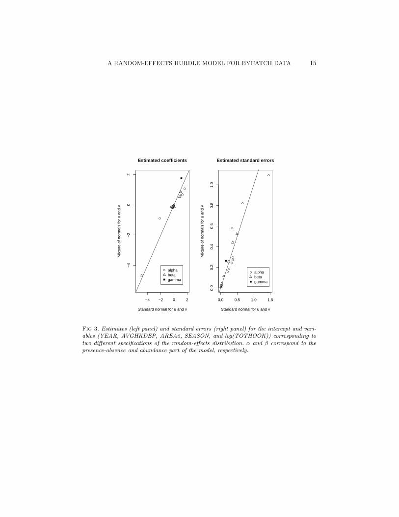
To better understand the coverage of the prediction intervals in Figure 2we revisit the random-effects’ distributional assumptions. In Table 1 we seethat the estimates for σu and σv are quite large with σv overestimated inthe independent hurdle model. McCulloch & Neuhaus (2011) have suggestedthat for the goal of predicting the random effects one can expect only modestimpacts on the mean squared error of prediction due to misspecification.For confirmation we did a sensitivity analysis (as summarized in Figure 3)where we assume mixtures of normal distributions for the predicted randomeffects (as suggested by their empirical distributions) and found that theestimated coefficients and corresponding errors are generally robust to thesemisspecifications.


−4 −2 0 2

−4

−2

02

Standard normal for u and v

Mix

ture

of n

orm

als

for

u an

d v

alphabetagamma

Estimated coefficients

0.0 0.5 1.0 1.5

0.0

0.2

0.4

0.6

0.8

1.0

Standard normal for u and v

Mix

ture

of n

orm

als

for

u an

d v

alphabetagamma

Estimated standard errors

Fig 3. Estimates (left panel) and standard errors (right panel) for the intercept and vari-ables (YEAR, AVGHKDEP, AREA5, SEASON, and log(TOTHOOK)) corresponding totwo different specifications of the random-effects distribution. α and β correspond to thepresence-absence and abundance part of the model, respectively.


4. Simulation Study. We carried out a simulation study to assesswhether parameters are estimated accurately using our methodology as wellas to understand the properties of our cluster-specific predictions. We sim-ulated data from our hurdle model (2.1)–(2.4). Each simulated data setcomprised c = 100 clusters, half with 5 measurements and half with 10 mea-surements per cluster, for a total of 750 observations. We included in xij anintercept, aN(0, 1) covariate and a Bernoulli(1/2) covariate (all independentof each other). The covariates zij included an intercept, the same N(0, 1)variable as in xij , a Bernoulli(1/2) variable and another N(0,1) variable, sothat xij and zij were partially overlapping. For each of 400 simulations, weused K = 1000 for the Monte Carlo approximation to the likelihood, 10starting points for its numerical optimisation and took B = 1000 in the fastbootstrap.

For the parameters, we considered four settings:

• Setting I: α = (0.5, 0.5, 1)T , β = (−0.5, 0.5, 1, 0.5), γ = 1, σu = 0.75and σv = 0.5, which gives 30% zeros on average.

• Setting II: Same as Setting I but with γ = 0.• Setting III: α = (−2, 0.5, 1)T , β = (−0.5, 0.5, 1, 0.5), γ = 1, σu = 0.75

and σv = 0.5, which gives 75% zeros on average.• Setting IV: Same as Setting III, but with γ = 0.

Setting III produces smaller, simplified versions of the bycatch data; theother settings are included to allow comparison with simpler situations.

4.1. Results for parameter estimation. In interpreting the results of fit-ting models for data with excess zeros, it is important to keep in mind that,although in general it is more difficult to fit models with random effectsto binary data (i.e. the presence-absence part) than to count data (i.e. theabundance part), fewer observations contribute to estimation of the param-eters in the abundance part of the model than the presence-absence part,so, in general, it tends to be more difficult to estimate and make inferencesabout the abundance parameters.

Figure 4 presents boxplots of the sampling distributions of the centeredparameter estimates for Settings III and IV (analogous results for SettingsI and II are given in the Supplementary Material, Figure 1). For the depen-dent hurdle model, all the regression parameters are estimated unbiasedlyin all four settings. The dependence parameter γ is also estimated approxi-mately unbiasedly, but has quite large variability. The spread parameters σuand σv are slightly underestimated on average when γ 6= 0 (Settings I andIII), but this is expected given the negative bias associated with maximumlikelihood estimation of variance components. The larger bias and variance


α1 α2 α3 β1 β2 β3 β4 γ σu σv

−1.

0−

0.5

0.0

0.5

1.0

dependent hurdle model − Setting III


−1.

0−

0.5

0.0

0.5

1.0

dependent hurdle model − Setting IV


−1.

0−

0.5

0.0

0.5

1.0

independent hurdle model − Setting III


−1.

0−

0.5

0.0

0.5

1.0

independent hurdle model − Setting IV

Fig 4. Setting III and IV: boxplots of (θl − θl) for l = 1, . . . , 10.

in the estimates of σv relative to σu are due to the smaller contributingsample sizes.

For the independent hurdle model, some of the regression parameter esti-mates are biased when γ 6= 0 (Setting I) and particularly in Setting III whenthe proportion of zeros is larger. This finding agrees with observations bySu et al. (2009), who considered two-part models for semicontinuous data,as well as those of Fulton et al. (2015), who modelled multivariate binaryresponses. As noted, an incorrect assumption of independence between therandom parts of the model produces biases in the parameter estimates, inparticular, the intercept for the abundance part, because correlated randomeffects are informative about cluster size (since parameters in the binary partinfluence the number of observations in the abundance part of the model).


Table 2

The couple (l, r) represents the percentage of confidence intervals that miss the truevalue, on the left (l) and on the right side (r), for a nominal 95% confidence interval.

Since 400 simulations were run each percentage must be a multiple of 0.25%. If the truevalue of l and r is 2.5% then the simulation standard error of their estimates is 0.78

percentage points. Similarly, if the true coverage is 95% the simulation standard error ofan estimate of coverage or non-coverage is 1.09 percentage points. (SE-H, standarderrors from the numerical Hessian; SE-b, standard errors from the bootstrap; boot.,

bootstrap percentile method.)

Setting III Setting IVdependent hurdle model indep. hurdle dependent hurdle model indep. hurdle

SE-H SE-b boot. SE-H SE-b boot.α1 (3.75, 1.75) (3.75, 1.50) (2.00, 1.25) (3.00, 2.75) (4.00, 1.50) (4.25, 2.00) (1.75, 1.50) (4.50, 1.50)α2 (1.75, 2.50) (2.50, 2.75) (0.50, 3.00) (2.75, 3.25) (2.75, 3.50) (2.25, 4.25) (1.25, 4.25) (2.50, 3.75)α3 (2.50, 3.00) (3.00, 3.25) (0.50, 3.50) (3.25, 4.25) (2.25, 3.50) (3.00, 3.00) (0.75, 4.00) (2.00, 3.25)σu (2.00, 3.75) (3.00, 5.75) (1.25, 5.75) n.a. (1.25, 3.25) (1.50, 3.25) (0.50, 3.25) n.a.β1 (3.25, 3.00) (3.75, 3.50) (2.00, 3.25) (2.50, 2.75) (2.00, 3.00) (2.25, 4.00) (1.25, 3.25) (2.75, 3.00)β2 (2.75, 2.50) (4.00, 5.00) (1.75, 5.50) (2.75, 3.00) (2.25, 3.00) (3.50, 3.75) (1.50, 3.25) (2.00, 3.25)β3 (2.75, 1.50) (4.25, 4.50) (1.25, 4.50) (3.50, 3.00) (2.75, 2.50) (4.25, 3.25) (1.00, 3.50) (2.50, 2.50)β4 (3.00, 1.25) (5.00, 3.75) (1.25, 4.25) (2.25, 3.00) (3.25, 4.00) (3.50, 4.50) (1.25, 4.00) (3.00, 4.00)σv (13.50, 15.25) (17.25, 30.00) (12.50, 30.75) n.a. (0.50, 5.00) (1.25, 10.00) (0.50, 9.25) n.a.γ (1.25, 14.50) (5.50, 16.50) (2.00, 17.00) – (2.00, 3.50) (3.50, 6.25) (0.75, 6.00) –

Further, when γ = 0 (Settings II and IV), the independent hurdle model iscorrect, but our dependent hurdle model performs as well as the independenthurdle model.

Table 2 shows the complement of coverage of 95% confidence intervalsfor Settings III and IV (analogous results for Settings I and II are given inthe Supplementary Material, Table 1). For the dependent model such inter-vals are constructed using (i) a normal approximation with standard errorestimates obtained from either the numerical Hessian or the bootstrap, or(ii) the bootstrap percentile method. For the independent hurdle model, anormal approximation is used with the (numerical) standard errors fromthe glmmADMB output. For the dependent hurdle model, the three methodsgive similar results. For the regression parameters α and β the confidenceintervals have good coverage and are fairly symmetric. Results are less sat-isfactory for the parameters related to the random-effects structure wheremissing to the right is more probable (due to the underestimation of thevariances) and the coverage is below the 95% nominal level. These parame-ters are more difficult to estimate; in particular σv and γ are more variablebecause they are estimated only from the nonzero observations which are asmall proportion of the total number of observations. In Setting IV, whereγ = 0, the actual coverage is better. For the independent hurdle model,only the standard errors for the regression parameters are available from


glmmADMB. The same comments apply for Settings I and II.One clear advantage of our model is the ability to perform tests on γ. In

fact, our simulation results support the use of a simple significance test (t-test). For a 5% nominal level, the actual level of such a test can be deducedfrom the confidence interval results. That is, for Setting II and IV (basedon the standard errors from the numerical Hessian, for example) the actuallevels are: 6.5% for Setting II and 5.5% for Setting IV. In cases where γ isfound to be non-zero we should always favor our dependent hurdle model asfailing to do so by using instead the independent hurdle model could leadto incorrect conclusions regarding the fixed-effects. We did explore bothlikelihood ratio testing and information criterion based procedures as alter-natives here but difficulties in establishing their distributions (in particularthe appropriate degrees of freedom) necessarily precluded their use.

4.2. Results for prediction. For a prediction target t(ui, vi,xij,zij,θ) wedecompose the mean squared error of prediction as

msepi = E{Tt(xij,zij, θ;yi)− t(ui, vi,xij ,zij ,θ)

}2

= E[Tt(xij ,zij , θ;yi)− E{Tt(xij,zij, θ;yi)}

]2

+[E{Tt(xij ,zij , θ;yi)} − E{t(ui, vi,xij,zij,θ)}

]2

+E [E{t(ui, vi,xij,zij,θ)} − t(ui, vi,xij ,zij ,θ)]2

= se{Tt(xij,zij, θ;yi)}2 + bias2 + sd{t(ui, vi,xij ,zij,θ)}2,and we estimate se, bias and sd empirically via 5%-trimmed means of the 400predictions obtained by simulation. Results for predictions in four distinctclusters (two with ni = 5 and two with ni = 10) are given in the Supplemen-tary Material, Tables 2-9. The bias is generally quite small, but more oftennegative. This is due to the underestimation of the spread parameters andthe built-in shrinkage effect in optimal prediction. There is reasonable agree-ment between

√msep (estimated using 5%-trimmed means) and

√msep∗t

(5%-trimmed mean of√msep∗), but with some exceptions.

Finally, in Table 3 we present the actual coverage of the normal predic-tion intervals (constructed by normal approximation using the bootstrapestimates of msep) for ui and vi for these clusters. There is good coveragefor ui, but not so good for vi, when γ 6= 0 (Settings I and III) because vi isestimated from a smaller sample.

5. Discussion. In this paper we propose a random-effects hurdle modelfor bycatch data and address all aspects of estimation, prediction and in-ference. In so doing we make available much anticipated tools for marine


Table 3

Actual coverages of nominal 95% prediction intervals for ui and vi.

CI(ui, ui) CI(vi, vi)Setting I II III IV I II III IVCluster 1 (ni = 5) 0.955 0.970 0.978 0.978 0.895 0.948 0.900 0.922Cluster 2 (ni = 5) 0.928 0.945 0.968 0.962 0.910 0.955 0.932 0.950Cluster 51 (ni = 10) 0.952 0.962 0.952 0.958 0.908 0.975 0.922 0.948Cluster 52 (ni = 10) 0.958 0.948 0.950 0.958 0.918 0.950 0.912 0.910

conservation research, specifically to predict cluster-specific targets like theprobablity of bycatch of endangered hammerhead sharks for particular fish-ing trips. Although we develop our estimation, prediction and inference pro-cedures for a random-effects hurdle model, they are easily adapted to abroad variety of situations. In fact, they can be used to obtain predictionsand their mean squared errors for the entire class of generalized linear mixedmodels and models with multiple mixed linear predictors, where no alterna-tive methods are currently available. As well, our general model formulation(Supplementary Material) contains numerous special cases for the randomstructure, including, for example, a two-level nested structure.

The random effects, used to describe the dependence structure of bycatchdata, are parametrized so as to be independent, which is convenient fornon-Gaussian random effects and, additionally, allows dependence betweenthe two parts of the model to be both optional and simply tested. For ourbycatch data, the dependence parameter is found to be significantly differentfrom zero, leading us to conclude that the random process determining thepresence/absence of bycatch is not independent of that determining the sizeof the nonzero bycatch events. As a result it would be inappropriate tomodel the nonzero bycatch events separately as is often done in practice.Further, our data analysis and simulation results demonstrate that ignoringthis dependence can lead to bias in the fixed-effects regression parameters aswell as an inability to predict random effects in some cases. In fact we wouldunderestimate both the extent to which the probablity of hammerhead sharkbycatch events is decreasing with time and the size of these events.

We derive empirical best predictors and obtain estimates of the meansquared error of these predictions using a fast bootstrap approach. Valuableinsight can be gained from these predictions and their variability. For exam-ple we can predict the probability of nonzero bycatch for particular trips aswell as the expected number of hammerhead sharks in these events. A com-prehensive simulation study demonstrates the effectiveness and reliability ofour proposals, for both the fixed-effects and the predictions. In particular,we see that the asymptotic theory applies well for the fixed-effects regres-


sion parameters but that the parameters of the random structure are moredifficult to estimate. For the random-target predictions, we observe acrosssimulations almost no bias and mean squared error estimates that are veryoften in agreement with those computed by bootstrap. Prediction intervalsconstructed using normal approximations are found to be reliable.

A natural next step is to incorporate spatially structured random effectsinto our framework so that we can more fully describe the spatial dependencein bycatch data and more accurately identify bycatch hotspots.

6. Acknowledgements. We thank the referees, Editor and AssociateEditor for helpful comments. This research has been supported by the Natu-ral Sciences and Engineering Research Council (Canada) and the AustralianResearch Council (DP0559135).

SUPPLEMENTARY MATERIAL

Supplementary material for the paper “A random-effects hurdle

model for predicting bycatch of endangered marine species”:

(doi: 10.1214/00-AOASXXXXSUPP; .pdf). The supplementary file containsfour sections. In the first section we give a general formulation of the ran-dom effects hurdle model. The second section presents a result about maxi-mum likelihood estimation of the model. The third section introduces a fastbootstrap estimator and establishes its asymptotic distribution. Finally thefourth section gives additional simulation results, as discussed in this paper.

References.

Alfo, M. & Maruotti, A. (2010). Two-part regression models for longitudinal zero-inflated count data. Canadian Journal of Statistics 38, 197–216.

Baum, J. (2007). Population- and community-level consequences of the exploitation oflarge predatory marine fishes. Ph.D. thesis, Biology Department, Dalhousie University,Halifax, Canada.

Baum, J., Myers, R., Kehler, D., Worm, B., Harley, S. & Doherty, P. (2003).Collapse and conservation of shark populations in the northwest atlantic. Science 299,389–392.

Booth, J. G. & Hobert, J. P. (1998). Standard errors of prediction in generalized linearmixed models. Journal of the American Statistical Association 93, 262–272.

Breslow, N. E. & Clayton, D. G. (1993). Approximate inference in generalized linearmixed models. Journal of the American Statistical Association 88, 9–25.

De Bruijn, N. G. (1981). Asymptotic Methods in Analysis. Dover, New York.Dobbie, M. J. & Welsh, A. H. (2001). Modelling correlated zero-inflated count data.

Australian & New Zealand Journal of Statistics 43, 431–444.Fournier, D. A., Skaug, H. J., Ancheta, J., Ianelli, J., Magnusson, A., Maunder,

M., Nielsen, A. & Sibert, J. (2012). AD Model Builder: using automatic differ-entiation for statistical inference of highly parameterized complex nonlinear models.Optimization Methods and Software 27, 233–249.


Fulton, K. A., Liu, D., Haynie, D. L., Albert, P. S. et al. (2015). Mixed model andestimating equation approaches for zero inflation in clustered binary response data withapplication to a dating violence study. The Annals of Applied Statistics 9, 275–299.

Furrer, R., Nychka, D. & Sain, S. (2012). fields: Tools for spatial data. R packageversion 6.6.3.

Hall, M. A., Alverson, D. L. & Metuzals, K. I. (2000). By-catch: problems andsolutions. Marine Pollution Bulletin 41, 204–219.

Huber, P., Ronchetti, E. & Victoria-Feser, M. (2004). Estimation of generalized lin-ear latent variable models. Journal of the Royal Statistical Society: Series B (StatisticalMethodology) 66, 893–908.

Hur, K., Hedeker, D., Henderson, W., Khuri, S. & Daley, J. (2002). Modelingclustered count data with excess zeros in health care outcomes research. Health Servicesand Outcomes Research Methodology 3, 5–20.

Jiang, J. (2003). Empirical best prediction for small-area inference based on generalizedlinear mixed models. Journal of Statistical Planning and Inference 111, 117–127.

Jiang, J. (2007). Linear and generalized linear mixed models and their applications.Springer Verlag.

Jiang, J., Jia, H. & Chen, H. (2001). Maximum posterior estimation of random effectsin generalized linear mixed models. Statistica Sinica 11, 97–120.

Jiang, J. & Lahiri, P. (2001). Empirical best prediction for small area inference withbinary data. Annals of the Institute of Statistical Mathematics 53, 217–243.

Jiang, J., Lahiri, P., Wan, S.-M. et al. (2002). A unified jackknife theory for empiricalbest prediction with m-estimation. The Annals of Statistics 30, 1782–1810.

Lambert, D. (1992). Zero-inflated Poisson regression, with an application to defects inmanufacturing. Technometrics 34, 1–14.

Lee, Y. & Nelder, J. (1996). Hierarchical generalized linear models. Journal of theRoyal Statistical Society. Series B (Methodological) 58, 619–678.

Lele, S. R., Dennis, B. & Lutscher, F. (2007). Data cloning: easy maximum likelihoodestimation for complex ecological models using bayesian markov chain monte carlomethods. Ecology letters 10, 551–563.

Lewison, R. L., Crowder, L. B.,Read, A. J. & Freeman, S. A. (2004). Understandingimpacts of fisheries bycatch on marine megafauna. Trends in Ecology and Evolution19, 598–604.

Liu, L., Strawderman, R., Cowen, M. & Shih, Y. (2010). A flexible two-part randomeffects model for correlated medical costs. Journal of Health Economics 29, 110–123.

McCulloch, C. E. & Neuhaus, J. M. (2011). Misspecifying the shape of a randomeffects distribution: why getting it wrong may not matter. Statistical Science 26, 388–402.

Min, Y. & Agresti, A. (2002). Modeling nonnegative data with clumping at zero: Asurvey. Journal of the Iranian Statistical Society 1, 7–33.

Min, Y. & Agresti, A. (2005). Random effect models for repeated measures of zero-inflated count data. Statistical Modelling 5, 1.

Molas, M. & Lesaffre, E. (2010). Hurdle models for multilevel zero-inflated data viah-likelihood. Statistics in Medicine 29, 3294–3310.

Mullahy, J. (1986). Specification and testing of some modified count data models.Journal of Econometrics 33, 341–365.

Myers, R., Baum, J., Shepherd, T., Powers, S. & Peterson, C. (2007). Cascadingeffects of the loss of apex predatory sharks from a coastal ocean. Science 315, 1846–1850.

Neelon, B., Ghosh, P. & Loebs, P. F. (2013). A spatial poisson hurdle model for


exploring geographic variation in emergency department visits. Journal of the RoyalStatistical Society: Series A (Statistics in Society) 176, 389–413.

Pikitch, E., Santora, C., Babcock, E., Bakun, A., Bonfil, R., Conover, D., Day-

ton, P., Doukakis, P., Fluharty, D., Heneman, B., Houde, E., Link, J., Liv-ingston, P., Mangel, M., McAllister, M., Pope, J. & Sainsbury, K. (2004).Ecosystem-based fishery management. Science 305, 346–347.

R Development Core Team (2011). R: A Language and Environment for StatisticalComputing. R Foundation for Statistical Computing, Vienna, Austria. ISBN 3-900051-07-0.

Rabe-Hesketh, S., Skrondal, A. & Pickles, A. (2002). Reliable estimation of gener-alized linear mixed models using adaptive quadrature. The Stata Journal 2, 1–21.

Salibian-Barrera, M., Van Aelst, S. & Willems, G. (2008). Fast and robust boot-strap. Statistical Methods and Applications 17, 41–71.

Skaug, H., Fournier, D., Nielsen, A., Magnusson, A. & Bolker, B. (2012). Gen-eralized Linear Mixed Models using AD Model Builder. R package version 0.7.4.

Su, L., Tom, B. D. M. & Farewell, V. T. (2009). Bias in 2-part mixed models forlongitudinal semicontinuous data. Biostatistics 10, 374–389.

Welsh, A., Cunningham, R. & Chambers, R. (2000). Methodology for estimating theabundance of rare animals: seabird nesting on north east herald cay. Biometrics 56,22–30.

Yau, K.& Lee, A. (2001). Zero-inflated poisson regression with random effects to evaluatean occupational injury prevention programme. Statistics in Medicine 20, 2907–2920.

E. Cantoni

Research Center for Statistics and

Geneva School of Economics and Management

University of Geneva

Bd Pont d’Arve 40

CH-1211 Geneva 4, Switzerland

E-mail: [email protected]

J. Mills Flemming

Department of Mathematics and Statistics

Dalhousie University

Halifax N.S., Canada, B3H 3J5


A. H. Welsh

Centre for Mathematics and its Applications

Australian National University

Canberra, ACT 0200, Australia


Documents

A RANDOM-EFFECTS HURDLE MODEL FOR PREDICTING …