A PROGRAMING MODEL

FOR CORPORATE FINANCIAL MANAGEMENT

by

Stewart C. Myers and Gerald A. Pogue

638-73January 1973

_.r-�..:-:-.�-l�=�-----��-^i--i--rl-.. ;-I-.--1.-;.I^-;--·I�--11--1� -�.-�..1.___��_^. .-.1.

A PROGRAMMING MODEL

FOR CORPORATE FINANCIAL MANAGEMENT

by

Stewart C. Myers and Gerald A. Pogue

I. INTRODUCTION

The theory of financial management now includes detailed con-

siderations of investment and financing decisions, of dividend policy,

and of most other aspects of corporate finance. But there is a clear

tendency to isolate these decisions in order to analyze them. To take

a simple example, consider the capital budgeting rules which depend

on an exogenous "cost of capital." These must assume that the firm's

financing decision is taken as given or is independent of the investment

decision, even though neither theory or practical considerations support

such a separation.

Financial management really requires simultaneous consideration

of the investment, financing, and dividend options facing the firm. The

purpose of this paper is to present a mixed-integer linear programming

model which includes these decisions and their interactions. The model is

based-on recent advances in capital market theory, but at the same time it

recognizes certain additional considerations that are manifestly important

to the financial manager. Thus, we believe that the model has both theoreti-

cal interest and the potential for practical application.

Before plunging into detail, it may be helpful to state the main

features of our approach in very general terms.

__ - ------ - -- ------ - I - - - " - - -

-2-

The linear programming model follows from two propositions of

modern capital market theory, namely:

(1) That the risk characteristics of a capital investment oppor-

tunity can be evaluated independently of the risk character-

istics of' the firm's existing assets or other opportunities.

(2) The Modigliani-Miller result that the total market value of

the firm is equal to its unlevered value plus the present

value of taxes saved due to debt financing.

Thus, the firm is assumed to choose that combination of invest-

ment and financing options that maximizes the total market value of the

firm, specified according to the two axioms. The major constraints are

a debt limit (specified as a function of the value and risk characteristics

of the firm's assets and new investment) and a requirement that planned

sources and uses of funds are equal. In addition, there are constraints

on liquidity, dividend policy, investment choices (due to mutually ex-

clusive or contingent options), etc. We do not argue that every one of

these additional constraints will be relevant in a practical situation,

rather we have included them for the sake of completeness.

The model has several important features:

(1) The objective is specified in terms of the firm's market

value, not in terms of someone's utility function.

(2) There is no restriction on the risk characteristics of the

investment opportunities considered.

(3) The model does not rely on the weighted average cost of capital,

and thus avoids the difficulties associated with that concept.

-3-

(4) .The model is linear in the decision variables, thus avoiding

the computational difficulties associated with non-linear

2programming. It requires mixed integer programming for ~

solution, but practical size problems can be efficiently

handled with existing computer codes.

Of course no model for overall financial management can or

should be entirely original -- our contribution is the combination of in-

gredients, not the ingredients themselves. Our debt to many other

authors will be evident as we' present the model piece by piece.3

c

- - ----- ---- ~_ _ -x-i~nru -a~9~-~ ----- `--

-4-

II. OBJECTIVE FUNCTION

The objective is to maximize the current market value of the

net worth of the firm, and thereby to maximize the wealth of current

shareholders. The market value of net worth at the beginning of period

t will be written as NWt, and the objective is thus to maximize NW1.

The firm is, of course, faced with certain immediate decisions.

But in general NW1 will also depend on future financing and investment

opportunities and the firm's future financial strategy. Thus, the problem

*is to find the optimal financial plan for the present (t = ) and for

future periods out to a horizon period (t = 2, 3, . . ., H).

Perfect capital markets will be assumed except for the imper-

fections specifically included in the model.

1: Decision Variables

We assume that management has identified a series of investment

opportunities, or projects, including both current and future opportunities.

The decision variables are:

1, if project k is accepted

xk 0, if project k is rejected.

The firm also has the opportunity to place funds in liquid

assets (marketable securities):

Lt = dollar investment in liquid assetsat the start ofperiod t

The major financing decisions are the amount and type of debt issued,

the amount of equity issued, and total cash dividends paid. For the case of

debt,

Y P dollar value of debt issued at the start of t,ti

in risk class i.

_ ~~~~~_~~ __ _ ~ ~ 1_ -11 ._ _ 1 _ __,,,_..._11 __ -1 ... . . I -- -- - - I -.,- _ -1 __ I · 1-1- 11-l-- --., -- ---------. -- -1_ __- _--

-5-

The second subscript on Y is needed because the risk of debt (to the

lender) depends on the firm's total debt obligation relative to its debt

capacity. T.us, the interest rate charged the firm will be a function

of the total debt issued. This is handled in the model by assuming that

the firm can issue a certain amount of prime debt (i = 1), but that to

issue more the firm must switch to medium grade (i 2), and so on. For

analytical convenience it is assumed that debt in each risk class is sub-

ordinate to debt of higher grades.

We could add a third' subscript to distinguish debt options by

their type and maturity. Clearly, management has to distinguish 5-year

from 20-year loans; but it might also be that a 5-year loan from a bank

has, say, a different repayment schedule from a 5-year note issued via an

underwriter. In order to simplify the presentation of the model we ignore

these considerations in this section of the paper, and assume that the firm

is concerned only with the total stock of debt outstanding in t, not its com-

position.

The decision variables for dividend and equity issues are

Et = amount of equity issued at the start of t

Dt ' dollar value of dividends paid at t.

There are a number of other variables in the objective functions --

various slack variables, for example, and also variables introduced to re-

flect the implicit costs of violating certain constraints. For example, man-

agement may wish to assign a cost to deviations from a target dividend pay-

ment. However, we will not discuss these variables further at. this point

since their rationale depends on the model's constraints.

--- ~ ~ _ ~ 1I__ _ __ _ X1 ~ _

-6-

2. The Status Quo

Usually the firm will have existing assets and liabilities taken

as given for purposes of analysis. This is included in the model by speci-

fying certain "autonomous" variables which are forced into the solution. The

thexisting assets are treated as the 0 project, with X =-1. The existing

debt levels in various risk classes are given by Yi', where Yi is con-

strained equal to the actual debt outstanding in class i.

Similarly, D and L represent existing levels of dividend pay-

ments and liquid assets respectively.

3. Form of the Objective Function

In the most general sense the objective is to maximize W 1,

which is a function of the k's, Lt's, Y D t s and Et's. The prob-

lem is to specify NW1 as a linear function of these variables.

Investment Decisions

We will begin with the "base case" of (1) all-equity financing,

(2) no liquid assets, and (3) irrelevance of dividend policy. The third

condition is defined in the sense of the well-known Miller-Modigliani proof [11],

which in the present context implies that NW1 is independent of the

D 's and E 's. In this case we propose thatt t

N

NWI Xk Ak X4(2-1)k=l

where Ak is the net present value of project k evaluated at the start of t = 1.

This specification rests on two assumptions. The first is "risk

independence," i.e., that risk characteristics of capital investment

-- - -, .'_ .... ... _ _ __ _ _ _ _ - '' - . .... ; _ -, . ., T ---n l-·-. ...... - ···- -·-- - ·- ·-- --·-_ - - ·- ··---_ _ - ·

-7-

opportunities can be evaluated independently of the risk characteristics

of the firm's existing assets or other opportunities. This means that

the market value of a portfolio of projects is equal to the sum of the -;

market values of the individual projects (assuming the projects could

be split off from the firm and separately financed). It also means that

diversification is more efficiently and flexibly accomplished within

investors' portfolios than within the firm.

There are several proofs that risk independence is a necessary

condition for equilibrium in perfect security markets.

The second assumption underlying Eq. (2-1) is the absence of

causal or "physical" interdependencies between project cash flows. Under

this assumption we must rule out competitive or complementary projects.

Obviously, if adoption of project j reduced the cash returns of project

k,'then would depend on X and Eq. (2-1) would not hold. However,

caosal interactions can be treated by introducing dummy projects whose

acceptance is contingent on adoption of the interacting projects. This

is discussed in detail later in the paper.

The important thing about Eq. (2-1), besides its linearity, is

that it makes no special assumptions about the risk characteristics of

investment projects. The manager computes A taking project k's risk

into account and then runs the model.

Of course, the model does not specicv how the value of each

investment opportunity is to be computed. For practical pruposes, we

propose

tCo( tA Ck(t) (2-2)

t-l t-l(1 + P)

_ ������� ��__�� _�_� �__..1... .... .����-�-�-------·- -·------------ -·-----�

-8-

where: O = the cost of capital for project k, assuming the basek

case of all-equity financing,dividend irrelevance, etc.

Pk is not a weighted average cost of capital.

Ck(t) = the expected after-tax cash flow from project k in t.

Ck(t) < 0 indicates a net cash outflow (investment). All

cash flows are assumed to occur at the beginning of

the period.

Debt Financing

Now we add the debt options:

N H II y F1

NW 1 OXk+ t:0 i YTi FTiK 0 T= i=l

where F is the present value per dollar. of class i debt issued in T,Ti

computed at the start of period 1. The variables for T 0 O refer to

the firm's existing debt.

Since the investment options are evaluated in terms of the base

case of all-equity financing, we must interpret Z YTi F as the in-T i

crease in current net worth due to a planned shift from all-equity finan-

1,cing to a mixed capital structure. Calculation of the FTi s must there-

fore be based on some theory of optimal capital structure. Although the

model does not rest on any particular theory (except for the assumption

of linearity) the Modigliani-Miller (MM) theorn is the natural choice

since we have assumed perfect capital markets. MM state that the total

value of the firm is equal to its unlevered value plus the present value

of tax savings due to debt financing.6

%4

(2-3)

..

I

r:; ·c ~ ~ ~ ~ ~ --·· I-- 1 1- - I-- - __ , -,-- - - - , I -I 1

9-

This idea can be implemented in the present context by a simple

discounted present value calculation. To simplify exposition, we will

assume that the borrowing rates pi are expected to be constant during the

firm's planning horizon. In this section we are not concerned with the ma-

turity of debt issued, and we can analyze debt issued in t as if it had

to be repaid or refinanced in t + 17 Thus Yti is interpreted as the total

stock of "new" debt in class i that is outstanding from t to t + 1.

(There may also be "old," that is autonomous, debt still outstanding, denoted

by Y0i.) Then we can write down the after-tax cash flows and discount

these flows back to period 1 at Pi, the prevailing interest rate for class

i debt.

Thus,

1 fti(t) fti (t+l)F (2-4)tt = (l+Pi) t-l (l+pi)t

where fi (t) is the general notation for the after-tax cash flows occurring

in t per dollar of class i debt issued in .

Equation (2-4) looks more complicated than it really is. The

immediate effect of issuing $1 of debt is a $1 cash inflow. Thus ft(t) = 1.

But there is a cash outflow the -next period which is to interest plus

principal repayment less the tax shield on interest. Thus,

fti(t + 1) = - (1+ pi) + T Pi

where TC is the marginal corporate tax rate. Discounting back to the

start. of period 1,

t . .. .~~~~~~.

· ___��1_�1__��__�_ _���__�__��_�

- 10 -

1 TCPiF = (2-5)ti 1PL

(1 + p )t

This is precisely the present value of tax savings due to $1 of class i

debt issue in t.

Eq. (2-5) rests on the assumption that the firm borrows at the

prevailing interest rate Pi, and the market capitalizes the tax shield

TC Pi at the same rate. This is reasonable since the firm can realizeC i

the tax shield only if the firm can pay the nterest. Thus the tax

9shields and interest payments have similar risk characteristics.

Bankruptcy Costs

At this point we must recognize an issue left unclear in the

MM propositions. If the choice between debt and equity is irrelevant

except for tax savings, then why not finance with 99.99 percent debt?

In our opinion there is no simple response, but we can recognize three

10limits that are practically important, namely (1) capital rationing,-

(2) managerial risk aversion and (3) bankruptcy costs. The first two

items would be reflected in debt capacity constraints (discussed below)

and do not affect the objective function. Bankruptcy costs, however, do

enter the objective function,

We interpret "bankruptcy costs" broadly, including not only the

costs of bankruptcy and reorganizations, but also any otherwise suboptimal

actions taken by the firm in order to avoid balL&ruptcy. The costs are re-

lated to planned debt commitments in the various debt classes.

For example,. assume the firm plans to have $1 of debt outstanding

in class 2, period 1. (Class i = 1 debt is assumed to be prime and thus leads

to low and perhaps negligible bankruptcy costs) We impute a cost of, say, $0.02.·

-li .--- - - - - - - -

- 11 -

to this liability. This amount is the decline in the market value of the

firm due to the possibility of bankruptcy due to the debt commitment.ll

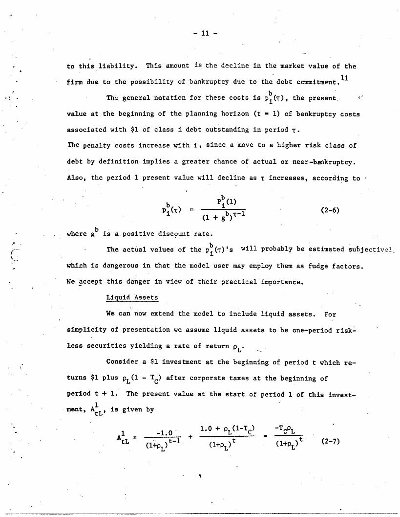
bTh'n. general notation for these costs is pi(T), the present.

value at the beginning of the planning horizon (t - 1) of bankruptcy costs

associated with $1 of class i debt outstanding in period T.

The penalty costs increase with i, since a move to a higher risk class of

debt by definition implies a greater chance of actual or near-bankruptcy.

Also, the period 1 present value will decline as T increases, according to 0

bPi(1)

pi(T) b (2-6)(1 + gb)T-1

bwhere g is a positive discount rate.

The actual values of the pi(T)'s will probably be estimated sutjectivel.

which is dangerous in that the model user may employ them as fudge factors.

We accept this danger in view of their practical importance.

Liquid Assets

We can now extend the model to include liquid assets. For

simplicity of presentation we assume liquid assets to be one-period risk-

less securities yielding a rate of return pL.

Consider a $1 investment at the beginning of period t which re-

turns $1 plus PL(1 - TC) after corporate taxes at the beginning of

period t + 1. The present value at the start of period 1 of this invest-

ment, AL, is given by

1 1.0 + pL(1-TC -TL1 - 01.0 L C C2LA = +tL (1+P 1 PLt (1+p)t (2-7)

~~( Pn tL (i+O L))

---------�· ��(�_II__· --����---I^____�_�__�____

- 12 -

1Note that AtL will be negative for reasonable values of pL

and T The reason is that liquid assets are equivalent to negative debt:

1 1if L Pl, then AtL = -Ftl, as can be seen by comparing Eqs. (2-5)

and (2-7). The liquid assets create an additional tax rather than a

tax shield. The fact that debt and liquid assets have mutually offsetting

effects on NW means that L must be a bit less than p1 to insure that

the model has a determinant solution. However, this makes sense since

the liquid assets are considered riskless; whereas the first class of

debt, while "prime," is not absolutely risk free.

Dividend Policy and Equity Issues

If we now add dividend and equity issue decisions to the factors

already discussed, we have

K- ~N . H INW1 -Xk Ai+ E Y Ti [F Ti + P

k=O T=O i=l

(2-8)H H H+ E L A + E P e()E + Z P d(T)D

-o=0 Tl T

where the last two terms are the effects of planned equity issues and

dividend policy, respectively, on the market value of net worth.

The model does not rely on any specific theory of optimal

dividend policy, except for the assumption of linearity. However, the

natural starting point is again the MM theory. According to M's proof, 1 2

dividend policy is irrelevant (i.e., it does not affect shareholders'

wealth) assuming investment policy is given. Any change in dividend

payment can be offset by a change in the amount of equity issued cr

S

- 13 -

shares repurchased, and the change in cash dividend received by the firm's

shareholders is exactly offset by a capital gain or loss due to the issue or

retirement of shares. In our model, this implies p (T) = pd(T) = 0. That is,

given values for the Xk's, the planned values of Et and Dt have no effecton NW1.

However, there is at least one market imperfection that cannot be

ignored: the transaction costs associated with new equity issues. Thus, we

e 13interpret p (T) as the cost per dollar of equity issued in period , with

epe(T) = p (l) (2-9)(l+ge T-1

eThe discount rate g reflects the fact that issue costs are better delayed,

simply because of the time value of money. Another complication is that total

issue costs are not a strict linear function of the amount of equity issued.

There is a substantial fixed cost associated with any issue, for example.

( . . Thus, we must turn to a piecewise linear function with Fe (T) representing the

fixed cost and v (T) the variable cost per dollar of equity issued. We also

erequire an equity issue decision variable, Zt, which takes the value zero if

no equity is issued in period t and one otherwise. This is discussed more

fully in the next section.

Although we know that equity issues are undesirable, it is less clear

how dividend increases affect NW1. Some would make p d(T) positive be-

cause of market imperfections or irrationality. We are more inclined to

the view that p () is negative due to unfavorable tax treatment of cash

dividends relative to capital gains income. That is, we interpret pd(T)

as the extra taxes paid by the firm's shareholders when they received a

dollar of cash income in T instead of a dollar of capital-gains.. However,

it is difficult to prove either view empirically.1 4

__�_�_�_�_���-x� -"-Lcl·� ��--------

- 14 -

Informational Content of Dividends and Reported Earnings

There is one more consideration which enters into the objective

function. So far we have assumed that investors have access to the same

information about the firm's plans and prospects as do the firm's mana-

gers. This is often not true; consequently, we must interpret NW1 as

the intrinsic value of the firm's net worth, and recognize that the actual

market value may not equal NW1 when information is limited.

This sort of market imperfection makes it hard to specify the

firm's objective with absolute clarity. Nevertheless, it seems more

reasonable and natural to maximize intrinsic value than any evident

alternative. In fact, the large corporation -- providing limited liability

and a means for delegation of financial decision making authority -- seems

(i. a natural response, given the task of maximizing value in the face

of informational limitations.

The major difficulty arises when pursuit of intrinsic value

leads to systematically false signals. Suppose the firm undertakes a large

and attractive investment. It cuts the dividend payment to finance the

investment. The probable result is a temporary drop in stock price, since

the dividend cut will be interpreted as a sign of management pessimism

about future earnings. The price will stay at a depressed level until

the true situation comes to light, and in the meantime shareholders

may sell at unfairly low prices.

A related problem is that most large investments generate rela-

tively little reported income during an initial "start-up" period (which

may last several years). This does not necessarily indicate a poor in-

vestment decision, but rather a bias ;:n the calculation of accounting%

.I.- ~~ -__1 11 -, ·'111' -

- 15 -

income. Thus, adoption of a project can generate a false signal con-

cerning the firm's long-run earnings.

There are basically two ways cr reacting to this sort of

problem. One is to tell the market the true cause for the low earnings

or dividend decrease. The other is to rearrange the firm's financial

decisions so as to maintain dividends and reported earnings. The

choice between these two strategies depends on the feasibility of the

former versus the cost of the latter.

In our model there are two sets of constraints which allow

management to "cost out" the policies of smoothing dividends and reported(This follows Chambers [3a] and Lerner and Rapoport [8].)

earnings. / The constraints establish target dividend and reported earn-

de reings growth rates, gd and gr and impose penalties pj cT) and t if

( the target levels are not met.

p C(T) is the present value at the start of period 1 ofj

penalty costs associated with $1 of dividend cut in period . The pen-

alty depends on the amount of the cut in steps indicated by = 1,

·, P.

Similarly, p (T) is the cost as of period 1 per dollar

penalty class j reported earnings reduction in period T.

Summary

Now we can put all of these pieces tqgether. The objective

function is to maximize the intrinsic value of 'W 1, the firm's net worth,

evaluated at the start of t = 1. NW1 is the sum of

(1) The present value of the firm's investments evaluated assuming

perfect markets and all-equity financing.'I

%

��_�_1�·__1_ __I __ _1__�_1_(_�_1_^__1_��-

- 16 -

(2) Plus the net present value of investments in liquid assets.

(3) Plus the present value of debt financing versus all-equity

final,cing, due to tax savings, net of bankruptcy costs.

present value of transaction(4) Minus the posta:-of planned equity issues (fixed plus variable

costs).present value of

(5) Minus the/tax penalties associated with dividend payments.

(6) Minus penalties assessed when target growth rates for dividends

and reported earnings are not met.

The next section presents a detailed discussion of the decision

variables and constraints associated with the various net worth penalty

costs. Following this we present a complete algebraic expression for

the objective function.

- 17 -

III. THE CONSTRAINTS

As discussed above, the goal of financial planning is to select

a financial plan which will maximize the value of the shareholder's equity.

The financial plan consists of a set of investment and financing decisions

covering the planning horizon of the firm. In this section we define the

restrictions on the set of feasible plans. These constraints can be

grouped into six categories, as follows.

(1) Cash flow constraints, insuring that planned sources and uses of

funds are equal.

(2) Debt capacity: these constraints limit the amount of debt the firm can

issue in various risk classes.

(3) Liquidity reserve: these constraints ensure that sufficient "slack"

exists in the financial plan to provide protection against the un-

certainties associated with projected cash requirements. The "slack"

takes the form of a liquidity reserve, composed of unused borrowing

capacity plus the liquid assets held by the firm.

(4) Investment restrictions: these constraints are necessary to allow

physical dependencies among projects.

(5) Equity issue costs: these constraints are necessary to represent the

costs associated with new equity issues.

(6) Information effects: these constraints represent the costs associated

with "erratic" dividends and reported earnings.

We now proceed to a detailed discussion of each of the constraint

types. To assist the reader, a summary of notation is given in Table 3-1.

1.. Expected Sources and Uses Constraints

For every feasible financial plan, expected cash requirements

in each period must be exactly matched by sources of funds. Thus,

1_____�_1_ ____1��1____�_ �__���I�_____II____I ���_·.ll�-CI(..- �-- ------- �-X----- ·--I ��--�--�--�

18 -

Table 3-1

Summary of Major Variables Used

1. Decision Variables

Xk Project zero-one decision variable, k 0, 1, . . ., N.

Lt Stock of liquid assets in period t, t = 0, .. ., H.

Y ~i Amount of risk class i debt issued in period T.YTi

'T = O 1, . .., H; i 1, . . ., I.

Et Amount of equity issue in period t.

eZt Equity zero-one decision variable.

i

Dt Aggregate dividends paid in period t.

dAmount of penalty class dividend reduction in period T.

TJ

Qua Amount of penalty class j reported earnings reduction in period T.

2. Parameters: Investment Options

Present value at t of project k.

tt 1OAk Standard deviation of k; OAk =0, however.

Yt kkt Correlation coefficient between Ak and AO .

Ck(t) Period t after-tax cash flows.

t

Cck(t) Cumulative cash flows to period t, i.e., Z Ck(t)t-1

.

Ill

-.I ..I ------ ." --- -, ---, I - 111 -I ~ ; --, - -_ , , _ _ _

- 19 -

Table 3-1 (Continued)

Cck(t) Standard deviation of C k(t).

Ykt Correlation coefficient between Cck(t) and Cc(t) .

ok Discount rate for project k, assuming all- equity financing.

tREk Contribution of project k to reported earnings in year t.

A Present value at t per dollar of L.

PL Rate of return on liquid assets, before tax.

3. Parameters: Financing Options

tF Present value at t per dollar of class i debt issued in T.FTi

f{i(t) After-tax period t cash flow per dollar of class i debt issued

in T.

aTi Dollars outstanding in t per dollar of class i debt issuedT i

in T.

Sit Stock of class i debt in period t.

Zit

Pi

Maximum amount of class 1 through i debt in period t.

Interest rate on class i debt.

V

__�I � �� ��Ul_�rl_ ______�_

- 20

Table 3-1 (Continued)

4. Parameters: Net Worth

NWt Net worth at t.

TAt Total assets at t.

o(NWt) Standard deviation of NWt.

a(TAt) Standard deviation of TAt

5. Parameters: Penalty Costs

All penalty costs are present value as of the start of period t.

bPti()

v t (T)

t( r)

d

Ptj(T)

Bankruptcy costs per dollar of risk class i debt outstanding

in period T .

Variable issue costs per dollar of equity issued in period T

Fixed cost of equity issued in period T

Tax penalty per dollar of dividend payments in period T

Penalty cost per dollar of period T dividend reduction

(penalty class j)

Penalty cost per dollar of period T reported earnings reduction

(penalty class j) .

Target dividend growth rate.

Target reported earning growth rate.

-.-.lfl- -

- 21 -

expected sources and uses of cash must net to zero in each decision

period. That is,

After tax cash After tax cash Net proceedsflow from + flow from debt + of equityprojects options issued

Dividends Increase in-- = 0

paid liquid assets

Stated in terms of the specific decision variables, this relationship

becomes, for each period t = 1, . .. , H,

N t I1 Y fo(t) (3-1)Xk Ck(t) + Z Ti fTi(t) (3-1)

k=O T=O i=l

+E - Vt (t)] - ZetFt (t) - Dt - [Lt (1 + (1-T)L) Ltl] = 0

Note that the cash flows from the firm's existing projects and debt fi-

nancing are included in the equation as X 0 and Yi'

2. Debt Capacity Constraints

The amount and quality of the debt a firm can issue obviously depends on

the nature of its assets. The more claims the firm issues againts its

assets, the lower the quality (rating) of these claims and the higher the

rate of interest demanded by lenders.

We assume that the firm can issue claims in I successively riskier

debt classes. Thus, we must limit the amount of debt that the firm can

issue in each risk class to the amount acceptable to the

�� - --̂---·- -·-"··-""·�^1�-·�---��

. A.

- 22 -

market. In practical terms we are placing limits on the amount of

debt the firm can issue in the various bond rating categories, such as

AAA, AA, etc.

The approach used to structure the debt limit constraints

is to assume that the market will accept additional debt in a given

risk class (quality rating)'up to the point where the probability

that the firm could "get into trouble" reaches an unacceptable level.

We define trouble as a situation in which the real value of the firm's

assets is less than the book value of its liabilities. Thus, the debt

outstanding in each risk class must be limited to a raction of the

expected market value of total assets in each future period. The size of the

fraction will depend on the degree of uncertainty about the future

value of the firm's assets.

This is illustrated in Figure 3-1. The figure shows the distribu-

tion of- the market value of the firm's total assets at the beginning of period

t of the planning horizon. The Zlt and Z2t are the limits for class 1 debt

and class 1 plus class 2 debt, respectively. Total assets equal the sum

of the net worth (NWt) plus the stock of class 1 and class 2 debt

outstanding. In general, there would be i values of Zit, one for each

debt class.

The amount of risk class i debt 'outstanding in period t

is obtained by summing the amounts outstanding from issues in periods

150 (initial debt) through t. That is,

tS E Y (3 -2)it ri ' TiTWO

"I/

- 23 -

Figure 3-1

Debt Limit Based on the Uncertainty

About the Future Value of the Firm's Assets

P(TAt )

Probability of"Trouble"

l

I

Expected Total Assets

NWt + Sit + Szt

Value ofTotalAssets

�___l___ll___�_*_IC__) __I__.. -----.�I_� _�__�DC�____I�-�_.�__ll��i��C�IIIIII___ ___

III *1

-It

0 .

- 24 -

The amount of debt outstanding in each risk class is.

limited to a portion of expected total assets. The appropriate frac--

tion is obtained by restricting the amount of debt in the first i classes

such that the probability of "trouble" is equal to the maximum allowable

value. That is,

P(TAt < Zt) = i (3-3)

where Zit is the dollar limit on the first i classes of debt. In

principle, the probability limit ci is determined from the behavior of

the debt markets. We use ci and the statistical properties of TAt to

solve for the debt limit, Zti

From Eq. (3-3),

E(TAt) Zti + ki (TAt ) (3-4)

-1where ki is equal to F (ci), F being the cumulative probability distri-

16bution for TAt . Thus,t

ti E(TAt) - ki (TAt), (3-5)

Iwhere E(TAt) = E[NWt] + Z Sit (3-6)

i=l

2 2 2 tand (TA) = (NW) = a(A)

where At is the present value of the firm's portfolio of investmentp

projects in period t. Now

2 ipl' N N

(A) XkXkCov(, kk-0 k'=O

11

- 25 -

which is, of course, non-linear in the X's. However,

where Ykt is the correlation coefficient between A and t.

Therefore, CyTA XkCov). ( NN

Eq. (3-7) does not really eliminate non-linearities in the specification

of 2(~At ), since Yk depends on the projects accepted and thus is nott~t0 p

available ex ante. However, it is a tolerable linear approximation if

we can assume that the correlation between and At is equal to that

bhe present value of the firm's assets existing at

t 0(3-7) Thidoes is realistic if the firnonm's investment opportunificaties do not

call for v depentures inthe projects accepted aind thustries, or if such ventures

are small relative to the existing assets and other opportunities.

Substituting Eqs. (3-6)and (3-7) into (3-5) we have

I

Zti I E[NWt] + Z S -t k XYka ) (3-8)with k > k for all i. The =l on class i debt can now be expressed

with ki1 > k i for all i. The limit on class i debt can now be expressed

as - Sit + W = Zit -z (3-9)

where Wit is the unused class i-debt capacity in period t.

���__�__�__^�_I �___I · _��I^_II_1_1_UII_�__IL----_llll�-·�·------- �--��I---

- 26 -

3. Liquidity Reserve

The sources and uses equations are stated in terms of

expectations. However, given the uncertainties associated with project

cash flows, planned sources may be insufficient to meet actual cash re-

quirements in future time periods,. For any real firm, both management

and stockholders would wish to ensure that a sufficiently large liquidity

buffer is built into the financial plan to provide a degree of flexi-

bility in the face of uncertainties associated with future cash flows.

The liquidity reserve (LR) is composed of liquid assets plus unused

borrowing potential,I

LRt = L + Z Witi=l

(3-10)

The various components which make up future cash require-

ments were enumerated in Eq. (3-1). For purposes of this model, we

assume that uncertainty is confined to project cash flows, k(t).

The constraint implied by the liquidity reserve require-

ment is given by

PROB(R t < CSt + LRt) > l- (3-11)

where Rt the cumulative project cash requirements to period t

(a random variable);

CS -. the cumulative financing cash flows to period t (a

deterministic variable), and

et - the maximum acceptable probability of having insufficient

·cash available in periods 1 through t.

The constraint is formulated on a cumulative rather than a noncumulative

basis so that the statistical relationship among the period-by-period

III

". -' -.. .. - - 1 ._ .--, _ -11 _ - _ ___ _ __

- 27 -

project cash flows can be explicitly considered. Also, the cumulative

formulation avoids the problem of double-counting the same liquidity e-

serve against liquidity requirements in several periods.

From equation (3-11),

CSt + LRt -E(CR t) > hta(CRt), (3-12)

where h is equal to F (l-et ), F being the cumulative probability dis-t t

tribution for CRt. However, from equation (3-1) planned requirements

E(CRt) are equal to planned sources CSt; thus, (3-12) becomes

LRt > h (CRt),

or

ILRt - Lt + E Wit .> hta(Rt).

iMl t t(3-13)

It now remains

the uncertainties of the

to develop

cumulative

an expression for (CRt) in terms of

project cash flows. By definition

CRt

Therefore,

where ECk(t)

-6kt

S

NE Xk(t)

k-O

N

a(Rk) - k Xkakt [Cck(t)],k=O

= the cumulative after tax cash flows for periods 1through t for project k, and

- the correlation coefficient between C (t) and CR.We approximate Ykt by the correlation etween Ckit)and the autonomous cash flows CCO(t), using thesame reasoning: applied to -k in Eq. (3-7),

I(��_ ____���__ __ �111^-�---·1

- 28-

Finally, the expression for the liquidity reserve becomes

I N

t + it > h t C Xk kta(Ck(t))i=l k=0

(3-14)

tJ

Of course, Eq. (3-14) fs in some respects similar to Eqs. (3-8),

which limit planned debt levels. Both types of constraint protect the

firm from overcommitment in the face of uncertainty. But the constraints

are conceptually and practically different. The debt capacity con-

straints insure long-run solvency, but liquidity is by definition a short

run concept. Thus, Eqs. (3-14) preserves flexibility rather than n-

solvency, The size of the liquidity reserve is critical only for

the first few periods of the plan, in which management's ability to re-

spond to unexpected events is limited. A reasonable means of reflecting

this in the model is to let ht approach zero as t approaches H, the

horizon period.

Naturally, the definition of "short run" depends on the charac-

teristics of the firm's business, in particular the speed and cost of

revising investment plans and the predictability of future investment op-

17portunities.

4. Investment Project Constraints

The possibility that various interdependencies will exist among

the investment projects requires the inclusion of additional constraints

in the model. The most common interdependencies are mutual exclusion,

contingency relationships, and physical dependencies between project

cash flows.

-~~~~~~~ --- ~~~~~~~~~~~~~~~~~~~·-- . --··; · - - -- - -. I 1 1-. .

-29 -

If projects and k are mutually exclusive, then the constraint

xj + , < (3-15)

will ensure that only one project is accepted. (Remember that xj and xk

are constrained to integer values.) This type of constraint can also

be used to consider the possibility of accepting the same project now

or at some later time.

If project can be undertaken only if project k is accepted,

the constraint is

Xj C Xk (3-16)

Physical dependencies between project cash flows occur when

the cash flows associated with project j depend on whether project k is

accepted, or vice versa. Pairwise physical dependencies can be handled

by introducing a dummy project, w, which is included in the solution if

and only if both projects j and k are accepted. Thus X - 1 whenever

Xj = 1, and 0 otherwise.

1Let A represent the incremental present value obtained if

both projects J and k are accepted. A may be positive or negative.w

When A is positive, the model's "instinct" will always be tow

include project w. It is constrained from doing so by making the ac-

ceptance of project w contingent on the acceptance of both and k. That

is,

X < Xk and X < X (3-17)

When A is negative, the following constraint is required:W I

__I�_ __�

�_�__�_____�____��...-Y�-�,��-.�..

i

30-

X > Xj + Xk - (3-18)

That is, whenever Xj - = - 1, X must so80 equal 1.

Generalization of the treatment of physical dependencies to

higher order relationships is straightforward. Suppose project w

represents the effect of joint acceptance of M projects. If isW

positive, then

< Xj, j 1, . .. , M (3-19)

If A is negative,then

MX > Xj- (M + 1). (3-20)

An additional cause of project interdependencies results whnen

special resources used by several projects are rationed. The firm may

have a limited supply of managers to assign to the various projects

under consideration. Forexample} let

'd the amount of the scarce resource required byproject j (e.g., the number of managers required)

D - the total supply of the resource available.

Then if m projects compete for the scarce resource, total usage must be

limited to the amount D.

mdjXj < D. (3-21)

c . -.

I

III

- 31 -

5. Equity Issue Costs Constraints

Equity issue costs are composed of a fixed component F (T)

and a variable component v(T). For simplicity the variable cost rate

is assumed to be independent of the issue size. The issue cost re-

sulting from Et dollars of equity issued in period t is

ee eZt Ft (t) +.Et Vt (t),

ewhere Zt is equal to zero of Et equals zero, and one otherwise. To

insure this relationship we required

Et < Zt (3-22)

10 ewhere is a large number (e.g. 10 ). Thus, when Z is equal to zero,

te

Et = 0, and when Zt = 1 the values of Et are not limited by the con-

straint.

The market value of assets in period t, NWt, will include

the present value of (at t) all future equity issue costs. The expres-

sion for NWt will thus include the terms

H

[Z t~~~t

�.�..I���----.------·-------�----- , � �-�-------·--·---···�-�--�------

- 32 -

6. Informational Constraints

These constraints are used in the calculation of penalties

to be applied to the firm's net worth resulting from erratic dividend

and reported earnings policies. The effect of the constraints is to

induce the model to smooth dividend payments and reported earnings over

time. The formulation of the constraints for dividends and reported

earnings are similar. Thus, we shall not provide a detailed treatment of

both. Let D = the aggregate dividends paid in year t (t 0, 1,· H)

gd ~ the expected long-run growth rate of dividends.

The difference between the dividends paid and the target level

is equal to (1 + gd) Dt 1 Dt. The impact on the market price of the

firm's stock will increase with the magnitude of the reduction. Thus,

the difference can be divided into steps which will be penalized at

successively higher rates. 8

We begin by dividing any decrease in aggregated dividend pay-

dments into increments, At.tj

P

(1 + gd)Dt-l - Dt - Z tj (3-23)j1.

t 1, . . ., H

where AD is the amount of dividend reduction n the jth penalty classtj

( - 1, . . ., P). Note that if Dt > (1 + gd)Dtl then Atj will equal

zero for all values of j. The model assumes that dividend increases

beyond the target level are neither rewarded nor penalized.

- -- - ____ __ _ ~ ---_ _ _ L -. - · I III- 11 - ---- -, -__ -- -_ --- ----

- 33 -

The amount of dividend reduction in each penalty class is lim-

ited to a specific fraction of the base dividend level. The first penalty

class is for dividend increases less than the expected value, the rest

dfor dividend reductions. Thus, Atl < gdDt_ , and for j - 2, . . ., P,

ddti < GDt-l (3-24)tj _ jt-l

where 0j > 0 and ZO = 1. The concave shape of the penalty function

ensures that Ad reaches its upper bound before Ad takes on positiveH P

d dctvalues. NWt will include the term Z Z Atj Pt ) to reflect the

T-t j=l market value penalty associated with dividend reductions.

The penalty costs associated with reductions in reported earn-

ings are treated in the same manner. Reported earnings in period i are

given byN t I

REt k O Xk · REkt + Lt_- dL(t) Z Z YTidi( ) (3-25)~t k=O Xk=O i Tl

where REt 3 contribution to reported earnings of project k in year t;

dL(t) after-tax interest rate received in period t per dollarof liquid assets held during period t-l, and

dTi(t) 3 after-tax interest payments in period t per dollar ofrisk class i debt issued in period T.

The target reported earnings in period t are equal to (1 + gR)REt 1

Any decrease in expected earnings from the target level can be divided

reinto segments A which are penalized at successively higher rates.ti

Q 1(r(1 + g )RE - RE < (3-26)

g)r t-1 t i tjlj=1

%

___�__11_�_��^___�1___� �__^_1_1____�11�_�__1__�� �·^_1__�__1__1_�_�� ___���_�_

- 34 -

Where, as in the dividend case,

rtlAtl < grREt_l

A r

t < aREt-1 J-2, . . ., Q

j> .

The net worth in period t will be reduced by an amount

H Qz £ Ar reT=t =ltj t

reflecting the reporting-earnings reduction penalties.

Model Summary

We can now present a complete algebraic expression for the

net worth in period t.( .

N

k=O

H+ Z L At

'r=t t T

H I+ £ Z YTi

T-0 il

Ft

,ti

H. I+ E S Pt (T)

T=t i=l

H+ %rt

[Z F(t) + E v t(T) ]

Present value in period t ofproject and autonomous cash flows

Present value of liquid assets heldduring periods t through H

Present value of financing options

Present value of bankruptcy costs

Present value of equity issue costs

H

+ DTP ()t t

Present value of dividend tax penalty

I

(3-27)

NWt

ill

--··�111

- 35 -

H P d dc+ E A P )

T=t j tj tj

H Q+ . Q Ar re (C)

Tt j= TJ PtjTrt J~l

Present value of dividend reductionpenalties

Present value of reported earningsreduction penalties

The objective of the model is to maximize the net worth at

the beginning of period 1, NW1. The major constraints on the decision

variables are,

(a) Sources and Uses of Cash

N t I' ~Ck(t) E YTi f i ( t )

k=O =O T i

{+ Et[1 - v t(t)] F(t) - Ptt t t

(3.1)- Lt - (1 + (1 - T) )Lt}

(b) Debt Capacity

- Stock of class i debt in period t

Sit

t

W E = d

-i-(3.2)

- Limit for class i debt

Sit + Wit = Zit - Zi-lt (3.9)

for all values of i.

I

.

�_I____�� __�_I_ _ _

- 36 -

(c) Liquidity Reserve

I NL +EW > >htE a tLt wit- t _ Xk kt (Cck(t))

i=1 k=O

(d) Project Constraints

- positive interaction (A > 0)w

X < X j - , . . ., Mw - J

- negative interaction (A < 0)

Mx > x -w - i J

(3.13)

(3.19)

(3.20)(M + 1)

(e) Equity Issue Costs

Et < Zt · (3.22'

(f) 'Information Effects

- dividend cuts

P( g)D1D d (3.23:'

- (1 + gd)Dtl Dt < Z t--1 tj

dwhere Atj < j . Dj 1 (3.24'

- reported earnings reductionsQ

(1 + gr) REt_- RE t < (3.26i-i tj

rwhere At < aj REt_ (3.27

Each of the above constraints must hold for values of t from to the

)

)

)

)

horizon period H.

III

- 37 -

IV. INVESTMENT OPPORTUNITIES AND HORIZON CONDITIONS

Two important aspects of the model remain to be discussed

-- the completeness of the investment opportunity set and the conditions

at the end of the planning horizon.

Investment opportunity set

Thus far we have implicitly assumed that all investment

projects to be considered during the planning horizon can be identified

in project by project detail at the beginning of the planning period. As

a practical matter, this is impossible. While the financial manager

may be able to describe all potential investment projects in the early

years of the planning horizon, this will not be the case for the later

periods. At most, he will be able to describe the aggregate nature of

yet-to-emerge opportunities.

In the absence of interdependencies among various investment and

financing decisions, there would be no need for additional information about

these opportunities; however, the sort of interdependencies discussed in

this paper makes it impossible to ignore them, since the

likelihood of future opportunities will influence current investment and

financing decisions.

A practical solution is to define a series of yet-to-emerge

investment projects, one for each year of the planning horizon, from t-2

to t=H. These would represent the financial managers' best guesses as

to the new opportunities that will eventually arise for those years. The

magnitude, risk and duration of the cash flows would probably reflect

extrapolations of previous investment experience. The amount

of potential investment opportunities would likely increase for

___�_______�_ ·I a. · -- I ��L��-l.-`--- ���------�----·--------·------L--"--�..-.-.-��.-�--�---�

- 38 -

later periods in the planning horizon, complementing the managers'

declining detailed knowledge of specific projects. The result of this

approach is to permit the delay of commitments to specific future proj-

ects until later when more information becomes available.

To include these projects in the model, we define a series

of decision variables XN+t-l' for t=2, . . ., H. These variables are

continuous rather than discrete, allowing fractions of the total of

projected opportunities to be included in the financial plan. Other-

wise, these projects would be treated identically to the N identified

projects.

By including these projects we have prevented the apparent

"disappearance" of the firm in later periods due to the absence of speci-

fic projects. Without them the first period decisions would be biased by

the apparent short life of the firm. For example, if future opportunities

were ignored, the debt capacity of the firm would appear to decline and

the model would be forced to plan for early retirement of debt.

Horizon Conditions

Another set of problems arise from the fact that the model

looks ahead only a finite number of periods, whereas the firm will con-

tinue to exist well beyond that time. It is thus necessary to consider

how the myopic nature of the model effects the recommended financial

plan. That is, what biases will result in the plan from the finite

nature of the model, and how can they be corrected? Ideally, we would

like to interface the model with the periods beyong the horizon so that

decisions are made as if the planning horizon were infinite.

Ill

- 39 -

One problem arises when the model is extended to cover the

choice among debt maturities. In this case there will be issues with

repayment schedules extending beyond the horizon. Since longer ma-

turity debt options have higher net present values per dollar issued,

and since there are no debt capacity constraints beyond t=H, the model

will use maximum maturity options for financing extending beyond the

horizon. Thus, the horizon debt structure will be artificially

biased toward longer maturities.

To remove this bias we truncate all debt issued at the be-

ginning of period H+1. Thus, all debt extending beyond the horizon

is assumed to mature at the beginning of period H+1, even though the

interest rates are for longer maturity periods. With this change the

debt option net present values F (j is the coefficient for maturity

and type) will no longer bias the model toward longer-maturity instruments.

Truncation of debt at the planning horizon, however, will

result in a bias against longer-lived projects. This results from

eliminating th.e benefits of post horizon debt capacity, which will be

largest for longer lived projects.

The solution clearly requires an approximization for the

value of the post-horizon debt capacity related to each project. One

way to do this is to discount project k's post horizon expected cash

flows back to t=l at a weighted average cost of capital k' while con-

tinuing to discount pre-horizon flows at Pk, the appropriate rate

assuming all-equity financing. Specifically, we replace Eq. (2-2) with:

H c1 C(T)

Ai E + Z t.- (4.1)T=l (+Pk) T=H+l (l+pk)

��--_11. 1111111-������--------II··�.··�-� --�-�� 11���--.--I_^.__.--�-I X-_-·-II..____·�_X-^_1111-_�-_-

- 40 -

where k is the weighted average cost of capital for the project. We(from [15]) *

use the MM formula/to obtain k from k and Xk, a target debt ratio for

the project:

Pk P 0k(l - TXk). (4.2)

The effect of discounting pk rather than pk is to increase the present

value of post horizon cash flows (assuming Xk positive), thereby reflect-

ing-the proJect's contribution to post-horizon debt capacity. This

method is not exact, but the errors introduced should not be serious in

19the present context.

Beyond period H, and after the lifetimes of the yet-to-emerge

projects discussed above, we assume that the firm enters a steady state.

In this condition, it is assumed to invest in projects which make no

contribution to net worth. While it would be conceptually possi-

ble to specify the nature of post-horizon growth opportunities, in

practice this would be a nebulous affair. Also, given their re-

moteness, the effect on current decisions will tend to be small.

V. CONCLUDING REMARKS

Our purpose was to develop a model which would permit simultan-

eous consideration of the investment, financing and dividend options fac-

ing the firm. Financial theory has typically treated these as independ-

ent decisions. However, this has been at the cost of ignoring a number of

important interactions. The main considerations which lead to a requirement

for simultaneous solution are:

III

- 41 -

\ . (1) Corporate Debt Capacity, which depends on the total risk charac-

teristics of the asset portfolio and not on individual projects

per se.

(2) Liquidity requirements, based on the uncertainty of aggregate

portfolio cash flows.

(3) Fixed costs associated with equity issues.

(4) Project interdependencies and resource constraints.

(5) Informational problems associated with dividend and reported

earnings policies.

These considerations are present in most practical situations.

Given this, it is not possible to maximize the value of the firm through

simple sequential determination of investment, financing and dividend

decisions. Our approach has incorporated these interactions and uses

mathematical programming to obtain the jointly optimal set of decisions.

The approach has a number of distinct advantages in addition

to the simultaneous nature of the solution. The major ones are:

(1) There are no restrictions on project risk characteristics. The

model allows explicit treatment of project risk differences in both

the objective function and constraints.

(2) Debt capacity is based on project risk characteristics and not on

arbitrarily determined debt equity ratios.

(3) The liquidity reserve is similarly based on the risk of project

cash flow, and not on rules of thumb.

(4). The model uses mixed integer linear programming

in order to avoid the fractional project difficulties associated

I

�1__�11111-·�-···r�-�i �-�.��-·0�--�---��_

- 42 -

with ordinary linear programming. Computationally

efficient codes exist for practical size problems.

The model formulation has a number of minor problems and one more sig-

nificant difficulty.

(1) Minor problems result from the assumptions necessary to maintain

the linear structure of the debt capacity and liquidity reserve

constraints. Also, penalties associated with dividend and reported

earnings reductions are on an aggregate rather than per share

basis to avoid the non-linearities associated with per share cal-

culations. The latter is only a problem during periods when new

equity is issued.

(2) The more serious problem results from the non-sequential nature of

the model. The model treats the problem as a single rather than multi-

stage decision problem. That is, the model develops a complete

financial plan at the beginning of the planning horizon rather

than a set of decision rules which will guide the course of the plan

as new information becomes available. Thus, decisions for periods

2 through H do not reflect the opportunity to obtain new informa-

tion at the end of period 1, and hence will no longer be op-

timal when new information is received at the end of period 1. Of

course, there is no need actually to implement these decisions, since the

model can be re-run at the beginning of each year to produce an up-

dated financial plan.

Cf

11

W

FOOTNOTES

1. See Myers [17] for a detailed treatment of the weighted average cost

of capital and the errors that can retult from its use.

2. There are some minor exceptions (noted in Section III below) where

approximations must be made to maintain the linear structure.

3. In addition to specific references later in the paper, we must note

here our general reliance on several authors' work.

The basic linear programming framework for financial planning

under certainty was laid by Charnes, Cooper and Miller [3].

Weingartner 24) extended this approach to capital budgeting decisions,

and Ngslund [18] made progress in extending the Weingartner model to

conditions of certainty.

The financing side of the model relies heavily on Modigliani and

Miller's treatment of capital structure and dividend policy. [11,12,133

K. Although the analysis of the risk of investment projects is exo-

genous to the model, the model does rely on the nation of risk inde-

pendence introduced by Myers [15]. As Fama [4) and Hamada note [6],

risk independence also holds approximately in the capital asset

pricing model of Sharpe [23], Lintner [10] and Mossin [14].

Of course,. other optimization models have been proposed for finan-

cial planning,. but the ones we have seen (examples are Carleton [2],

Chambers [3a] and Moses [5)) do not share the essential features of

the model we are presenting here. By "essential features" we have

in mind particularly our reliance on modern capital market theory,

our treatment of risk differences among investment opportunities, and

our specification of debt capacity and liquidity constraints.

4. That is, it is assumed that the average interest rate with subordination

is the same, ceteris paribus, as if one undifferentiated class of debt

were issued. This seems to be a reasonable approximation given the

intent of the model. See Robichek and Myers [211, pp. 31-32 for a

theoretical justification.

-·--~~--~~~-·-~~-- ~ --------

Footnotes 2

5. See Myers [151, and Schall [.22]. The latter provides a review of

the literature on this subject.

The risk-independence concept, usually advanced with the firm's

investment decision in mind, applies to the financing decision as

well. (That is, the proofs apply to transactions either in real or

financial assets.) Thus, this concept also supports our use of a

linear objective function with respect to security issues and retirements.

6. See Modigliani and Miller [13], and Robichek and Myers [21].

7. For ease of exposition this one period debt assumption will be main-

tained throughout Section II. In later sections the discussion will

be generalized to debt of fixed, multi-period maturity.

8. There are no conceptual difficulties in expanding Eq. (2-4) to cover

various maturities, changing interest.rates across maturities and

time, etc.

9. Of course, this assumes that T is known, that the firm will have

taxable income in all future periods, etc. It also assumes the firm

always borrows at the going rate Pi. If this was not true for some

reason (example: government-subsidized fincnaing) then the present value

of the debt option would be computed from Eq. (2-4) rather than (2-5).

10. For discussion, see Jaffee and Modigliani [7] and the other sources

cited there.

11. Note that the bankruptcy costs are not due to imperfections in the

(secondary) securities markets. Rather, they are real costs (e.g.,

lawyer's fees) deducted from the firm's assets in the event of bank-

ruptcy. Thus, the introduction of bankruptcy costs here does not con-

flict with our reliance on perfect capital markets, the idea of

risk independence or with MM's bsic approach to the analysis of financ-

ing decisions.

III

Footnotes 3

12. Miller and Modigliani [11], esp. pp. 412, 415. The proof was in-

dependently presented by Lintner [9]; however, Lintner feels it appli-

cability is much more limited than M do.

13. These costs may also reflect the clientele effect stressed by

Lintner [9].

14. See Black and Scholes [1] for recent tests and references to earlier

work.

15. For the one period debt case the stock of class i debt outstanding

is given byt

it = oi Yoi + Yti

16. ki can be determined by assuming TAt is normally distributed, or from

a nonparzmetric relationship such as Tchebyscheff's inequality.

17. The need for the explicit inclusions of a liquidity reserve constraint

results from the single-stage nature of the model. Specifically,

the sources and uses constraints for t=l, . .. , H are based on ex-

pected (as of t=0) cash requirements. The liquidity reserve is re-

quired to insure that sufficient cash sould be available to meet the

actual requirements in period 2 and beyond. Without this reserve,

additional costs (not considered in the current objective function)

would be incurred in raising additional cash to meet the unanticipated

requirements. If the model had been formulated as a multi-stage de-

cision problem, explicit recognition would have been taken of the

requirements that could arise beyond the first period. The

optimal financial plan would then have build in liquidity reserves

to protect against higher than expected cash requirements. However,

for practical reasons, as well as ease of exposition we have chosen

not to follow te multi-stage approach. The data and computational re-

quirements for a full blown multi-stage approach are typically prohibi-

tive for problems of practical size. From an exposition point of view

formulating

--------��-� .�Y· �-YI·-� �XI·�-�l·-s_-_----��-�1��---�--�-��-�-_�

Footnotes 4

the model as a multi-stage linear programming problem would

simply add detail which would obscure discussion of the basic

issues. This approach is identical to that used by Pogue and

Bussard in their short term planning model [19].

18. Another approach to smoothing dividends and reported earnings is

commonly usad in analytical planning models (see, for example,

Lerner and Rappaport [8]). It involves simply constraining aggregate

values in each period to equal or exceed one plus the target growth rate

times the value in the previous period. The costs of these con-

straints are then evaluated through an examination of the relevant shadow

prices.

Our approach allows the model to "price out" reductions in divi-

dends and reported earnings. However, the simpler approach may be

more appealing in some applications.

19. See Myers [17], pp. 25-32.

···

·

~~~~~~~~~~~~~~~~~~~~~~~~~~~~~~~~~~~~~~~~~~~~~~~~~~~~~~~~~~~~~~~~~~~~~~~~~~~~~~~~~~~~~~~~~~~~~~~~~~~~~~~~~~~~~~~~~~~~~~~~~~~~~~~~~~~~~~~~~~~~~

··-·- ·- ·-·-- ---;---· ---·

REFERENCES

.1. Black, F. ad Scholes, M., "Dividend Yields and Common Stock Re-turns: A New Methodology," unpublished working paper, Sloan School

of Management, M.I.T. (1971)

2. .Carleton, Willard T., "An Analytical Model for Long Range FinancialPlanning," The Journal of Finance.

3. Charnes, A. A., Cooper, W. W. and Miller, M. H., "Application of

Linear Programming to Financial Budgeting and the Costing of Funds,"Journal of Business, January 1959.

3a. Chambers, D., "Programming the Allocation of Funds Subject to Restric-tions on Reported Results." Operational Research Quarterly, December 1967.

4. Fama, E., "Risk Return and Equilibrium: Some Clarifying Comments,"Journal of Fir.ance, March 1968.

5. Hamilton, . and Moses M., "An Optimization Model for Corporate Financial

Planning," unpublished working paper, Department of Industry, WhartonSchool of Finance and Commerce, University of Pennsylvania, January1971.

6. Hamada, R., "Portfolio Analysis, Market Equilibrium and CorporateFinance," Journal of Finance, March 1969.

7. Jaffee, D. M. and Modigliani, F., "A Theory and Test of Credit Ration-ing," American Economic Review, December 1969.

8, Lerner, E. M. and Rappoport,"Limit DCF in Capital Budgeting,"Harvard Business Review, September-October 1968.

9. Lintner, John, "Dividends, Earnings, Leverage, Stock Prices andthe Supply of Capital to Corporations," Review of Economics andStatistics, August 1962..

10. Lintner, J., "The Valuation of Risk Assets and the Selection of RiskyInvestments in Stock Portfolios and Capital Budgets," The Reviewof Economics and Statistics, Debruary 1962.

11. Miller, M. H. and Modigliani, F., "Dividend Policy, Growth and

the Valuation of Shares," Journal of Business, October 1961.

12. Modigliani F. and Miller, M. H., "The Cost of Capital, Corporation Financeand the Theory of Investment," American Economic Review, June 1958/

13. ,"Corporate Income Taxes and the Costof Capital: A Correction," American Economic Review, June 1963.

References 2

14. Mossin, J., "Equilibrium in a Capital Asset Market," Econometrica,October 1966,

15. Myers, S. C., "Procedures for Capital Budgeting Under Uncertainty,"

Industrial Management Review, Spring 1968.

16. , "A Note on Linear Programming and Capital Budgeting,"The Journal of Finance, March 972.

17. , "On-the Interaction of Corporate Financing and Invest-ment Decisions and the Weighted Average Cost of Capital," unpublishedworking paper, Sloan School of Management, M.I.T. #598-72, May 1972.

18. Ngslund, B., "A Model of Capital Budgeting Under Risk," The Journalof Business, Aril 1966.

19. Pogue, G. i. and Bussard, R. N., "A Linear Programming Model forShort Term Financial Planning Under Uncertainty," Sloan ManagementReview, Spring 1972.

20. Robichek, A. A. and Myers, S. C., Optimal Financing Decisions,I Englewood Cliffs, New Jersey, Prentice Hall, 1965.

.'f (< . - 21. _, "On the Theory of OptimalCapital Structure," Journal of Financial and Quantitative Analysis,June 1966.

22. Schall, L. D., "Asset Valuation, Firm Investment and Firm Di-ersifi-cation," Jurnal of Business, January 1972.

23. Sharpe, W. F., "Capital Asset rices: A Theory of Market EquilibriumUnder Conditions of Risk," Journal of Finance, September 1964.

24. Weingartner, M. H., Mathematical Programming and the Analysis of

Capital Budgeting, Englewood Cliffs, N. J., Prentice Hall, Ind.1963.

.

C

111