A procedure for the reliability improvementof the oblique ionograms automaticscaling algorithmAlessandro Ippolito1, Carlo Scotto1, Dario Sabbagh1,2, Vittorio Sgrigna2, and Phillip Maher3

1Istituto Nazionale di Geofisica e Vulcanologia, Rome, Italy, 2Dipartimento di Matematica e Fisica, Università degli StudiRoma Tre, Rome, Italy, 3Space Weather Services, Bureau of Meteorology, Sydney, New South Wales, Australia

Abstract A procedure made by the combined use of the Oblique Ionogram Automatic Scaling Algorithm(OIASA) and Autoscala program is presented. Using Martyn’s equivalent path theorem, 384 oblique soundingsfrom a high-quality data set have been converted into vertical ionograms and analyzed by Autoscala program.The ionograms pertain to the radio link between Curtin W.A. (CUR) and Alice Springs N.T. (MTE), Australia,geographical coordinates (17.60°S; 123.82°E) and (23.52°S; 133.68°E), respectively. The critical frequency foF2values extracted from the converted vertical ionograms by Autoscala were then compared with the foF2 valuesderived from themaximum usable frequencies (MUFs) provided by OIASA. A quality factorQ for theMUF valuesautoscaled by OIASA has been identified. Q represents the difference between the foF2 value scaled byAutoscala from the converted vertical ionogram and the foF2 value obtained applying the secant law to theMUF provided by OIASA. Using the receiver operating characteristic curve, an appropriate threshold level Qt

was chosen for Q to improve the performance of OIASA.

1. Introduction

Currently, the knowledge of the real-time state of the ionosphere relies on the application of assimilative techni-ques into both physical and empirical models. For this purpose, real-time ionospheric data are required.Interestingly, the Earth’s ionosphere was discovered by the observations of radio waves reflected by an unknownlayer. Following Marconi’s experiments, a number of pioneers of wireless [Kennelly, 1902; Heaviside, 1902; Lodge,1902] stated that waves properties could only be explained by the presence of a reflecting layer composed ofelectrons and positive ions. The existence of such a layer was demonstrated in 1925 by Edward Appleton togetherwith his studentMiles Barnett [Bibl, 1998]. In subsequent years, the techniquewas refined to the point of recordinga graph t(f) of the time t elapsed for a radio frequency f to travel the ionosphere-Earth-ionosphere path onto a film,the device being called an ionosonde. Networks of ionosondes are now routinely used to measure the character-istics of the ionosphere. Well-established techniques, such as the Automatic Real Time Ionogram Scaler with TrueHeight Analysis system [Reinisch and Huang, 1983; Gilbert and Smith, 1988; Galkin et al., 2008] and the Autoscalaprogram [Scotto and Pezzopane, 2002a, 2002b; Pezzopane and Scotto, 2007; Scotto, 2009], make it possible toobtain the main ionospheric characteristics, such as the critical frequencies of the different ionospheric layersand the related virtual heights, in real time from vertical ionograms [Scotto and Pezzopane, 2008]. The output dataprovided by these software packages can be integrated in real time and provide short term forecasting models[Galkin et al., 2012]. Unlike vertical soundings, for which transmitter and receiver are colocated, for oblique iono-spheric soundings the transmitter and the receiver are generally several hundreds or thousands of kilometersapart, such that the radio waves are obliquely incident on the ionosphere. The oblique ionogram that one obtainsfrom this kind of measurement (Figure 1a) is a representation of the time delay versus the frequency response ofthe ionosphere, for the considered radio link. The interpretation of ionspeheric parameters from oblique iono-grams is significantly more complex when compared to the vertical ionograms, and there are no well-establishedautomatic techniques. Oblique soundings are mainly used to understand the factors that attenuate and distortthe propagation of radio wave in the high-frequency (HF) range through the ionized layer of the Earths atmo-sphere, in order to improve radio link reliability caused by this natural variability of the ionosphere.

2. Automatic Scaling of Oblique Ionograms

In the absence of an automatic procedure for the interpretation of the oblique ionograms, time intensivemanual methods are required in order to individually scale them. However, with the growing interest in

IPPOLITO ET AL. QUALITY FACTOR FOR OIASA ALGORITHM 454

PUBLICATIONSRadio Science

RESEARCH ARTICLE10.1002/2015RS005919

Key Points:• A quality factor is defined for the MUFvalues provided by OIASA algorithm

• The oblique ionograms are convertedinto vertical and analyzed byAutoscala

• The quality factor is based on the foF2obtained by the autoscaling of thevertical ionograms

Correspondence to:A. Ippolito,alessandro.ippolito@ingv.it

Citation:Ippolito, A., C. Scotto, D. Sabbagh,V. Sgrigna, and P. Maher (2016),A procedure for the reliabilityimprovement of the oblique ionogramsautomatic scaling algorithm, Radio Sci.,51, 454–460, doi:10.1002/2015RS005919.

Received 11 DEC 2015Accepted 5 APR 2016Accepted article online 8 APR 2016Published online 17 MAY 2016

©2016. American Geophysical Union.All Rights Reserved.

the acquisition of real-time ionospheric data for correcting propagation delays in satellite communications, pre-dicting space weather, and ionospheric disturbances due to geomagnetic storms and solar flares [Jin et al., 2006;Cushley and Noel, 2014], this has highlighted the need for the automatic scaling of oblique ionograms [Redding,1996]. In addition, oblique ionospheric sounding also offers several important advantages over vertical sound-ing. For example, the opportunity of monitoring the ionosphere across large, otherwise inaccessible areas suchas ocean surfaces and the ability of a receiver to detect signals from many different directions. Despite the factthat oblique ionogram inversion methods have received less attention than the inversion of the vertical iono-grams, several attempts have been made in order to derive the midpoint electron density profile from obliquesoundings.Gething andMaliphant [1967] suggested a double-stepmethod inwhich an oblique ionogram is con-verted into a vertical and analyzed bymeans of inversion techniques developed for vertical ionograms. A furtherapproach is to obtain the electron density profile directly from the oblique ionogram, as has been proposed byPhanivong et al. [1995]. This method takes into account the presence of the Earth’s magnetic field and is basedon the inversion technique developed by Reilly and Kolesar [1989], which considers the curvature of the iono-sphere and handles the ambiguity related to the presence of the valley in the electron density profile. In thework presented here, we propose a quality factor for the MUF values provided by Oblique IonogramAutomatic Scaling Algorithm (OIASA) [Ippolito et al., 2015]. Applying OIASA to an oblique ionogram, we obtainthe autoscaled value of maximum usable frequency, MUF[OIASA], from which we derive the critical frequency ofthe F2 layer through the secant law. The autoscaled oblique ionogram is then converted into a vertical one andthen analyzed by the Autoscala program in order to obtain the critical frequency foF2. The two values of foF2,resulting from the two different procedures are then compared. The reliability of MUF[OIASA] is assessed in thisway, and a technique to discard the cases of erroneous interpretation is consequently introduced.

3. Oblique to Vertical Ionograms Conversion

The procedure to convert an oblique ionogram into a vertical one begins with the storage of the obliquesounding in matrix form. The number of rows m and columns n of the matrix A are defined by the followingformulas:

m¼ inttf � t0ð ÞΔt

� �; (1)

and

n¼ intf f � f 0ð ÞΔf

� �(2)

where int stands for integer; ff, f0, Δf, tf, t0, and Δt are, respectively, the final frequency, the initial frequency,the frequency step, the final time delay, the initial time delay, and the time delay resolution of theoblique sounding. The values t0 and Δt are fixed and depend on the design of the ionosonde. The valuesf0, ff, and Δf, are usually set in accordance with the programmed measurement campaign. The element aij

Figure 1. The results of the application of the noise filtering algorithm. An ionogram (a) before and (b) after the applicationof the noise filter.

Radio Science 10.1002/2015RS005919

IPPOLITO ET AL. QUALITY FACTOR FOR OIASA ALGORITHM 455

(with i= 1, …, m and j=1, …, n) of the matrix A isan integer ranging from 0 to 255; proportional tothe amplitude of received echo, this value isobtained directly from the data file recorded bythe instrument.

To reduce the radio frequency (RF) noise withoutaffecting important ionogram features, an addi-tional simple original algorithm has been devel-oped to filter the background noise from theimage. An example of the results obtained canbe seen in Figures 1a and 1b, in which is shownthe same ionogram before and after applyingsuch a filter algorithm. The filter algorithm ana-lyzes each element aij of the matrix A and, whenrecognized as a component of the noise, it is elimi-nated. Since image background noise is often pre-sented as dense sets of pixels, a defined number

of pixels, chosen with the nearest neighbor technique around the considered element aij, are analyzedand their numerical values are summed up. When this sum is greater than a fixed threshold, the elementaij is assumed to be part of the noise and then deleted. Once the ionograms background noise is filtered,every element aij of the matrix A represents a frequency-virtual ray path pair. Applying the secant law andthe Martyn’s equivalent path theorem [Martyn, 1935] to each element aij, the equivalent vertical ionogramis obtained. According to the geometry of the oblique ray path shown schematically in Figure 2, the curvatureof the Earth is also considered. Taking into account an isotropic, horizontally homogeneous, and flat iono-sphere and representing fo and fv as the frequencies of the radio waves reflected obliquely and verticallyrespectively, at the same real height, from the secant law we have

f v ¼ f osecϕ

; (3)

where ϕ is the incidence angle of the high-frequency radio signal. According to the Martyn’s theorem, thevirtual height at which fv is reflected from the ionosphere is given by [Gething, 1969; Kol’tsov, 1969]:

h′ f vð Þ ¼ p′ f oð Þ2secϕ

� c: (4)

Through geometric considerations we also have

c ¼ RT 1� cosθð Þ; (5)

and

ϕ ¼ sin�1D

p′ f oð Þ : (6)

where h′, c, RT, θ, p′, and D are, respectively, the virtual reflection height of the vertical signal, its correction forthe curvature of the Earth, the Earth radius, the angle at the center of the Earth, the group path of the obliquesignal, and the ground range associated to the oblique radio link. Combining the equations from (3) to (6), weobtain the conversion of the considered oblique ionogram into a vertical ionogram. This is done starting fromthe oblique ionogram in which for a frequency fo can be deduced p(fo). From p(fo) ϕ is obtained through (6),where D is known. The ϕ is introduced in (4) to derive h′(fv). Finally, fv is determined by (3).

4. Definition of the Quality FactorQ for the Improvement of the OIASA Performance

Besides the automatic interpretation of oblique ionograms, a further important issue of an autoscalingalgorithm is being able to discard ionograms that even an expert operator could not interpret. This criticalissue is also taken into account by the OIASA autoscaling algorithm. The contrast method used by OIASAto recognize the ordinary and extraordinary traces of ionospheric oblique soundings has proved to be also

Figure 2. A scheme of the considered geometry for an obliqueray path, where Tx and Rx represent, respectively, the transmitterand the receiver. The Earth’s curvature is also taken into account.

Radio Science 10.1002/2015RS005919

IPPOLITO ET AL. QUALITY FACTOR FOR OIASA ALGORITHM 456

a useful method for discarding ionograms lacking data or those that are excessively noisy [Ippolito et al.,2015]. In this method two empirical curves Tord and Text, which are able to fit the typical shape of the F2 traceon the oblique ionograms, are defined for the detection of the ordinary and extraordinary traces, respectively.The local contrast C between Tord and Text and A is then calculated making allowance for both the number ofmatched points and their amplitude. The curves Tord and Text having the maximum value of C are thenselected. If this value of C is greater than a fixed threshold Ct, the selected curves are considered as represen-tative of the traces due to reflection from the F2 region. Otherwise, no MUF value is provided as output, andthe ionogram is deemed to lack sufficient information and is discarded. In this work we define a quality factorfor the MUF values provided by OIASA, which will improve the reliability of the automatic scaling. The assess-ment of the false detections and the percentage of ionograms discarded is one of themain goals of this work:the results obtained will be discussed in the following and summarized in the conclusions. The equivalentvertical ionogram, resulting from the conversion of the original oblique ionogram, is stored in an RDF (RawData Format) file format and analyzed by Autoscala. This operation enables deriving all the ionospheric para-meters over the midpoint of the oblique ray path, as shown in the examples in Figures 3a–3c. Autoscala

Figure 3. (a, b, and c) Examples of oblique ionograms converted into verticals. The results of the application of Autoscalaprogram and the Adaptive Ionospheric Profiler (AIP) are also reported.

Radio Science 10.1002/2015RS005919

IPPOLITO ET AL. QUALITY FACTOR FOR OIASA ALGORITHM 457

uses empirical curves to fit the typical shape of the F2, F1, and Es [Scotto and Pezzopane, 2002a, 2002b;Pezzopane and Scotto, 2007, 2008; Scotto and Pezzopane, 2007] trace. Once different parts of the ionogramtrace have been automatically identified, the electron density profile is estimated by an iterative techniqueto best fit a 12 free-parameter electron density profile model, called Adaptive Ionospheric Profiler (AIP),with the recorded ionogram [Scotto, 2009]. The critical frequency foF2 given by Autoscala (foF2[Autoscala]) iscompared with foF2[OIASA], derived by the application of the secant law to the OIASA autoscaled MUF(MUF[OIASA]):

f oF2 OIASA½ � ¼MUF OIASA½ �

secϕ: (7)

The parameter Q=Δ foF2 = |foF2[Autoscala] – foF2[OIASA]| can be used, as shown in the next section, as a qualityfactor for the MUF values provided by OIASA. This can considerably decrease the false positive event occur-rence, namely, the percentage of those ionograms for which the absolute value of the difference betweenthe MUF obtained by OIASA and by a manual scaling procedure exceeds 1.5MHz. The proposed procedureis schematically shown in Figure 4. An electron density profile Ne(h) at the midpoint of the considered radiolink is also estimated through the described technique, using the Adaptive Ionospheric Profiler (AIP),[Scotto, 2009].

The performance of the procedure presented in this paper was tested using a set of 384 high-quality iono-grams, not previously filtered, from the Australian Bureau of Meteorology’s Space Weather Services (SWS)campaign of oblique soundings, performed on the 1218 km path between the ionosondes of CUR,Australia (17.60°S; 123.82°E) and MTE, Australia (23.52°S; 133.68°E). The SWS oblique ionograms wererecorded using a Digital Oblique Receiving System (DORS) on loan from the Australian Defence Scienceand Technology group (DST). As reported in Tables 1a and 1b, for all the ionograms of the data set, an experi-enced operator has been able to scale a MUF value which has been assumed as reference. We define as

Figure 4. The system flow diagram of the whole algorithm, in which the quality factor Q is defined and used in a filteringprocedure in order to decreases the false positive event percentage. Operations belonging to the procedure used to set thethreshold value Qt are marked by green arrows and boxes.

Table 1a. The Behavior of OIASA to Reject Ionograms With Insufficient InformationWithout Using Any Filtering Procedurea

Scaled by the Software Discarded by the Software

No. of Cases (%) No. of Cases (%)

The operator did not scale the MUF 0 0 0 0The operator scaled the MUF 384 100 0 0Total 384 0

aThe analyzed data set is made by 384 high-quality oblique ionograms taken by SWS.

Radio Science 10.1002/2015RS005919

IPPOLITO ET AL. QUALITY FACTOR FOR OIASA ALGORITHM 458

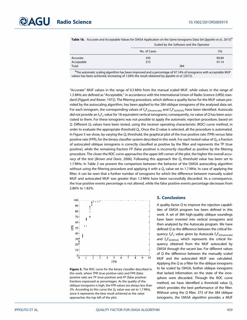
“Accurate” MUF values in the range of 0.5MHz from the manual scaled MUF, while values in the range of1.5MHz are defined as “Acceptable,” in accordance with the International Union of Radio Science (URSI) stan-dard [Piggott and Rawer, 1972]. The filtering procedure, which defines a quality factor for the MUF values pro-vided by the autoscaling algorithm, has been applied to the 384 oblique ionograms of the analyzed data set.For each ionogram, the corresponding values of foF2[Autoscala] and foF2[OIASA] have been identified. Autoscaladid not provide an foF2 value for 18 equivalent vertical ionograms; consequently, no value ofQ has been asso-ciated to them. For these ionograms was not possible to apply the automatic rejection procedure, based onQ. Different Qt values have been tested, using the receiver operating characteristic (ROC) curve method, inorder to evaluate the appropriate threshold Qt. Once the Q value is selected, all the procedure is automated.In Figure 5 we show, by varying the Qt threshold, the graphical plot of the true positive rate (TPR) versus falsepositive rate (FPR), for the binary classifier system described in this work. For each tested value ofQt, a fractionof autoscaled oblique ionograms is correctly classified as positive by the filter and represents the TP (truepositive), while the remaining fraction FP (false positive) is incorrectly classified as positive by the filteringprocedure. The closer the ROC curve approaches the upper left corner of the plot, the higher the overall accu-racy of the test [Brown and Davis, 2006]. Following this approach the Qt threshold value has been set to1.7MHz. In Table 2 we present the comparison between the behavior of the OIASA autoscaling algorithmwithout using the filtering procedure and applying it with a Qt value set to 1.7MHz. In case of applying thefilter, it can be seen that a further number of ionograms for which the difference between manually scaledMUF and autoscaled MUF was greater than 1.5MHz have been successfully discarded. As a consequence,the true positive events percentage is not altered, while the false positive events percentage decreases from2.86% to 1.82%.

5. Conclusions

A quality factor Q to improve the rejection capabil-ities of OIASA program has been defined in thiswork. A set of 384 high-quality oblique soundingshave been inverted into vertical ionograms andthen analyzed by the Autoscala program. We havedefined Q as the difference between the critical fre-quency foF2 value given by Autoscala foF2[Autoscala]and foF2[OIASA] which represents the critical fre-quency obtained from the MUF autoscaled byOIASA through the secant law. For different valuesof Q the difference between the manually scaledMUF and the autoscaled MUF was calculated.Applying the Q as a filter for the oblique ionogramsto be scaled by OIASA, further oblique ionogramsthat lacked information on the state of the iono-sphere were discarded. Through the ROC curvemethod, we have identified a threshold value Qt

which provides the best performance of the filter.Without using the Q filter, 373 of the 384 obliqueionograms, the OIASA algorithm provides a MUF

Table 1b. Accurate and Acceptable Values for OIASA Application on the Same Ionograms Data Set [Ippolito et al., 2015]a

Scaled by the Software and the Operator

No. of Cases (%)

Accurate 345 89.84Acceptable 373 97.14Total 384

aThe automatic scaling algorithm has been improved and a percentage of 97.14% of ionograms with acceptable MUFvalues has been achieved, increasing of 1.04% the result obtained by Ippolito et al. [2015].

Figure 5. The ROC curve for the binary classifier described inthis work, where TPR (true positive rate) and FPR (falsepositive rate) are TP (true positive) and FP (false positive)fractions expressed as percentages. As the quality of theoblique ionograms is high, the FPR values are always less than3%. According to this curve the Qt value was set to 1.7 MHz,since it represents the best result achieved as the valueapproaches the top left of the plot.

Radio Science 10.1002/2015RS005919

IPPOLITO ET AL. QUALITY FACTOR FOR OIASA ALGORITHM 459

value within the range of 1.5MHz from the manual scaled MUF, while no ionograms were automatically dis-carded. This resulted in 11 out of the 384 oblique ionograms deemed as being false positive events at a rateof 2.86%. When applying the Q filter, it was found that 373 of the 384 oblique ionograms had been scaled cor-rectly by the OIASA software (ΔMUF< 1.5MHz), 4 ionograms were automatically discarded and 7 were deemedto have been incorrectly scaled by the software (ΔMUF> 1.5MHz). In this case the false positive event percen-tage decreases from 2.86% to 1.82%. The algorithm described in this work is an efficient method to improve theperformance of OIASA, which can be proposed as a system to obtain the real-timeMUF fromoblique ionograms.

ReferencesBibl, K. (1998), Evolution of the ionosonde, Ann. Geofis., 41, 667–680.Brown, C. D., and H. T. Davis (2006), Receiver operating characteristics curves and related decision measures: A tutorial, Chemom. Intell. Lab.

Syst., 80, 24–38.Cushley, A. C., and J.-M. Noel (2014), Ionospheric tomography using ADS-B signals, Radio Sci., 49, 549–563, doi:10.1002/2013RS005354.Galkin, I. A., G. M. Khmyrov, A. V. Kozlov, B. W. Reinisch, X. Huang, and V. V. Paznukhov (2008), The ARTIST 5, in Radio Sounding and Plasma

Physics, AIP Conference Proceedings, vol. 974, pp. 150–159, doi:10.1063/1.2885024.Galkin, I. A., B. W. Reinisch, X. Huang, and D. Bilitza (2012), Assimilation of GIRO data into a real-time IRI, Radio Sci., 47, RS0L07, doi:10.1029/

2011RS004952.Gething, P. J. D. (1969), The calculation of electron density profiles from oblique ionograms, J. Atmos. Terr. Phys., 31, 347–354.Gething, P. J. D., and R. G. Maliphant (1967), Unz’s application of Schlomilch’s integral equation to oblique incidence observations, J. Atmos.

Terr. Phys., 29, 599–600.Gilbert, J. D., and R. W. Smith (1988), A comparison between the automatic ionogram scaling system ARTIST and the standard manual

method, Radio Sci., 23(6), 968–974, doi:10.1029/RS023i006p00968.Heaviside, O. (1902), Telegraphy, Encyclopaedia Britannica, Edimburgh.Ippolito, A., C. Scotto, M. Francis, A. Settimi, and C. Cesaroni (2015), Automatic interpretation of oblique ionograms, Adv. Space Res., 55, 1624–1629.Jin, S. G., J. U. Park, J. L. Wang, B. K. Choi, and P. H. Park (2006), Electron density profiles derived from ground-based GPS observations,

J. Navig., 59(3), 395–401, doi:10.1017/S0373463306003821.Kennelly, A. E. (1902), Research in telegraphy, Elec. World Eng., 6, 473.Kol’tsov, V. V. (1969), Determination of virtual reflection heights from oblique sounding data, Geomagn. Aeron. (USSR), 9(5), 698–701.Lodge, O. (1902), Mr Marconi’s results in day and night wireless telegraphy, Nature, 66, 222.Martyn, D. F. (1935), The propagation of medium radio waves in the ionosphere, Proc. Phys. Soc., 47, 323–339.Pezzopane, M., and C. Scotto (2007), The Automatic Scaling of Critical Frequency foF2 and MUF(3000)F2: a comparison between Autoscala

and ARTIST 4.5 on Rome data, Radio Sci., 42, RS4003, doi:10.1029/2006RS003581.Pezzopane, M., and C. Scotto (2008), A method for automatic scaling of F1 critical frequency from ionograms, Radio Sci., 43, RS2S91,

doi:10.1029/2007RS003723.Phanivong, B., J. Chen, P. L. Dyson, and J. A. Bennet (1995), Inversion of oblique ionograms including the Earth’s magnetic field, J. Atmos. Terr.

Phys., 57, 1715–1721.Piggott, W. R., and K. Rawer (1972), U.R.S.I. Handbook of Ionogram Interpretation and Reduction, US Department of Commerce National

Oceanic and Atmospheric Administration-Environmental Data Service, Asheville, N. C.Redding, N. J. (1996), The autoscaling of oblique ionograms, Research report DSTO-RR-0074.Reilly, M. H., and J. D. Kolesar (1989), A method for real height analysis of oblique ionograms, Radio Sci., 24, 575–583, doi:10.1029/

RS024i004p00575.Reinisch, B. W., and X. Huang (1983), Automatic calculation of electron density profiles from digital ionograms: 3. Processing of bottomside

ionograms, Radio Sci., 18(3), 477–492, doi:10.1029/RS018i003p00477.Scotto, C. (2009), Electron density profile calculation technique for Autoscala ionogram analysis, Adv. Space Res., 44(6), 756–766, doi:10.1016/

j.asr.2009.04.037.Scotto, C., and M. Pezzopane (2002a), A software for automatic scaling of foF2 and MUF(3000)F2 from ionograms, in Proceedings of URSI

2002, Maastricht, 17–24 August, 2002 (on CD).Scotto, C., and M. Pezzopane (2002b), A software for automatic scaling of foF2 and MUF(3000)F2 from ionograms, URSI XXVII General

Assembly. [Available at http://www.ursi.org/Proceedings/ProcGA02/papers/p1018.pdf.]Scotto, C., and M. Pezzopane (2007), A method for automatic scaling of sporadic E layers from ionograms, Radio Sci., 42, RS2012, doi:10.1029/

2006RS003461.Scotto, C., and M. Pezzopane (2008), Removing multiple reflections from the F2 layer to improve Autoscala performance, J. Atmos. Sol. Terr.

Phys., 70, 1929–1934.

Table 2. Comparison Between the Behavior of OIASA Without Applying the Filtering Procedure and Applying theFiltering Procedurea

Results Without Q Filter Results With Q Filter

No. of Cases (%) No. of Cases (%)

Well scaled (ΔMUF< 1.5 MHz) 373 97.14 373 97.14Bad scaled (ΔMUF> 1.5 MHz) 11 2.86 7 1.82Discarded 0 0 4 1.04Total 384 384

aThe Qt value of the filter is set to 1.7MHz. A data set of 384 high-quality oblique ionograms has been considered. Itcan be notice how the true positive events percentage is not altered, while the false positive events percentagedecreases from 2.86% to 1.82% .

AcknowledgmentsThe authors performed part of theresearch reported here while guests ofthe Space Weather Services of theAustralian Bureau of Meteorology. Theionogram data set used for this researchhas been provided by the AustralianDefence Science and Technology group(DST). The authors thank MurrayParkinson from SWC and RobertGardiner-Garden from DST for theircomments and suggestions. The dataused in this work can be request toAlessandro Ippolito (alessandro.ippoli-to@ingv.it).

Radio Science 10.1002/2015RS005919

IPPOLITO ET AL. QUALITY FACTOR FOR OIASA ALGORITHM 460