Embed Size (px)
Citation preview

A Probabilistic Generative Grammar forSemantic Parsing
Abulhair Saparov∗Carnegie Mellon University
Tom M. Mitchell∗Carnegie Mellon University
We present a framework that couples the syntax and semantics of natural language sentences ina generative model, in order to develop a semantic parser that jointly infers the syntactic, mor-phological, and semantic representations of a given sentence under the guidance of backgroundknowledge. To generate a sentence in our framework, a semantic statement is first sampled froma prior, such as from a set of beliefs in a knowledge base. Given this semantic statement, agrammar probabilistically generates the output sentence. A joint semantic-syntactic parser isderived that returns the k-best semantic and syntactic parses for a given sentence. The semanticprior is flexible, and can be used to incorporate background knowledge during parsing, in waysunlike previous semantic parsing approaches. For example, semantic statements correspondingto beliefs in a knowledge base can be given higher prior probability, type-correct statements canbe given somewhat lower probability, and beliefs outside the knowledge base can be given lowerprobability. The construction of our grammar invokes a novel application of hierarchical Dirichletprocesses (HDPs), which in turn, requires a novel and efficient inference approach. We presentexperimental results showing, for a simple grammar, that our parser outperforms a state-of-the-art CCG semantic parser and scales to knowledge bases with millions of beliefs.
1. Introduction
Accurate and efficient semantic parsing is a long-standing goal in natural languageprocessing. There are countless applications for methods that provide deep semanticanalyses of sentences. Leveraging semantic information in text may provide improvedalgorithms for many problems in NLP, such as named entity recognition (Finkel andManning 2009, 2010; Kazama and Torisawa 2007), word sense disambiguation (Tanakaet al. 2007; Bordes et al. 2012), semantic role labeling (Merlo and Musillo 2008), co-reference resolution (Ponzetto and Strube 2006; Ng 2007), etc. A sufficiently expressivesemantic parser may directly provide the solutions to many of these problems. Lower-level language processing tasks, such as those mentioned, may even benefit by incorpo-rating semantic information, especially if the task can be solved jointly during semanticparsing.
Knowledge plays a critical role in natural language understanding. The formalismsused by most semantic parsing approaches require an ontology of entities and predi-cates, with which the semantic content of sentences can be represented. Moreover, evenseemingly trivial sentences may have a large number of ambiguous interpretations.Consider the sentence “She started the machine with the GPU,” for example. Withoutadditional knowledge, such as the fact that “machine” can refer to computing devices
∗ Machine Learning Department, 5000 Forbes Avenue, Pittsburgh, PA 15213.E-mails: [email protected] and [email protected]
© 2005 Association for Computational Linguistics
arX
iv:1
606.
0636
1v1
[cs
.CL
] 2
0 Ju
n 20
16

Computational Linguistics Volume xx, Number xx
KBSemantic statement
turn_on_device(person:Ada,device:gpu_cluster)
Generative semantic grammar
Parser S
VP
NP
NPPNP
V
NP
“She started the machine with the GPU”“She started the machine with the GPU”
Figure 1High-level illustration of the setting in which our grammar is applied. During parsing, the inputis the observed sentence and knowledge base, and we want to find the k most probablesemantic-syntactic parses given this input and the training data.
that contain GPUs, or that computers generally contain devices such as GPUs, the readercannot determine whether the GPU is part of the machine or if the GPU is a device thatis used to start machines.
The thesis underlying our research is that natural language understanding requiresa belief system; that is, a large set of pre-existing beliefs related to the domain of dis-course. Clearly, young children have many beliefs about the world when they learn lan-guage, and in fact, the process of learning language is largely one of learning to groundthe meanings of words and sentences in these non-linguistically acquired beliefs. Insome ways, the idea that language understanding requires a belief system is not new,as natural language researchers have been saying for years that background knowledgeis essential to reducing ambiguity in sentence meanings (Bloom 2000; Anderson andPearson 1984; Fincher-Kiefer 1992; Adams, Bell, and Perfetti 1995). But despite thisgeneral acknowledgement of the importance of background knowledge, we see veryfew natural language understanding systems that actually employ a large belief systemas the basis for comprehending sentence meanings, and for determining whether themeaning of a new sentence contradicts, extends, or is already present in its belief system.
We present here a step in this direction: a probabilistic semantic parser that uses alarge knowledge base (NELL) to form a prior probability distribution on the meaningsof sentences it parses, and that "understands" each sentence either by identifying itsexisting beliefs that correspond to the sentence’s meaning, or by creating new beliefs.More precisely, our semantic parser corresponds to a probabilistic generative modelthat assigns high probability to sentence semantic parses resulting in beliefs it alreadyholds, lower prior probability to parses resulting in beliefs it does not hold but whichare consistent with its more abstract knowledge about semantic types of arguments todifferent relations, and still lower prior probability to parses that contradict its beliefsabout which entity types can participate in which relations.
This work is only a first step. It is limited in that we currently use it to parsesentences with a simple noun-verb-noun syntax (e.g. "Horses eat hay."), and considersonly factual assertions in declarative sentences. Its importance is that it introduces anovel approach in which the semantic parser (a) prefers sentence semantic parses that
2

Saparov and Mitchell A Probabilistic Generative Grammar for Semantic Parsing
yield assertions it already believes, while (b) still allowing with lower prior probabilitysentence interpretations that yield new beliefs involving novel words, and (c) evenallowing beliefs inconsistent with its background knowledge about semantic typingof different relations. We introduce algorithms for training the probabilistic grammarand producing parses with high posterior probability, given its prior beliefs and anew sentence. We present experimental evidence of the success and tractability of thisapproach for sentences with simple syntax, and evidence showing that the incorporatedbelief system, containing millions of beliefs, allows it to outperform state-of-the-artsemantic parsers that do not hold such beliefs. Thus, we provide a principled, prob-abilistic approach to using a current belief system to guide semantic interpretation ofnew sentences which, in turn, can be used to augment and extend the belief system. Wealso argue that our approach can be extended to use the document-level context of asentence as an additional source of background beliefs.
For reasons including but not limited to performance and complexity, most modernparsers operate over tokens, such as words. While this has worked sufficiently wellfor many applications, this approach assumes that a tokenization preprocessing stepproduces the correct output. This is nontrivial in many languages, such as Chinese, Thai,Japanese, and Tibetic languages. In addition, a large portion of the English vocabulary iscreated from the combination of simpler morphemes, such as the words “build-er,” “in-describ-able,” “anti-modern-ist.” Moreover, language can be very noisy. Text messages,communication in social media, and real-world speech are but a few examples of noiseobfuscating language. Standard algorithms for tokenization, lemmatization, and otherpreprocessing are oblivious to the underlying semantics, much less any backgroundknowledge. Incorporating these components into a “joint parsing” framework willenable semantics and background knowledge to jointly inform lower-level processingof language. Our method couples semantics with syntax and other lower-level aspectsof language, and can be guided by background knowledge via the semantic prior. Wewill demonstrate how this can be leveraged in our framework to model the morphologyof individual verbs in a temporally-scoped relation extraction task.
Semantic statements are the logical expressions that represent meaning in sentences.For example, the semantic statement turn_on_device(person:Ada, device:gpu_cluster) maybe used to express the meaning of the sentence example given earlier. There are manylanguages or semantic formalisms that can be used to encode these logical forms: first-order logic with lambda calculus (Church 1932), frame semantics (Baker, Fillmore, andLowe 1998), abstract meaning representation (Banarescu et al. 2013), dependency-basedcompositional semantics (Liang, Jordan, and Klein 2013), vector-space semantics (Salton1971; Turney and Pantel 2010), for example. Our approach is flexible and does notrequire the use of a specific semantic formalism.
In section 3, we review HDPs and describe the setting that we require to define ourgrammar. We present our approach in section 3.1.1 to perform HDP inference in thisnew setting. In section 4, we present the main generative process in our framework,and detail our application of the HDP. Although we present our model from a gen-erative perspective, we show in the description of the framework that discriminativetechniques can be integrated. Inference in our model is described in section 5. There, wepresent a chart-driven agenda parser that can leverage the semantic prior to guide itssearch. Finally, in section 6, we evaluate our parser on two relation-extraction tasks: thefirst is a task to extract simple predicate-argument representations from SVO sentences,and the second is a temporally-scoped relation extraction task that demonstrates ourparser’s ability to model the morphology of individual words, leading to improvedgeneralization performance over words. Moreover, we demonstrate that the inclusion
3

Computational Linguistics Volume xx, Number xx
of background knowledge from a knowledge base improves parsing performance onthese tasks. The key contributions of this article are:1. a framework to define grammars with coupled semantics, syntax, morphology, etc.,2. the use of a prior on the semantic statement to incorporate prior knowledge,3. and an efficient and exact k-best parsing algorithm guided by a belief system.
2. Background
Our model is an extension of context-free grammars (CFGs) (Chomsky 1956) thatcouples syntax and semantics. To generate a sentence in our framework, the semanticstatement is first drawn from a prior. A grammar then recursively constructs a syntaxtree top-down, randomly selecting production rules from distributions that dependon the semantic statement. We present a particular incarnation of a grammar in thisframework, where hierarchical Dirichlet processes (HDPs) (Teh et al. 2006) are usedto select production rules randomly. The application of HDPs in our setting is novel,requiring a new inference technique.
The use of the term “generative” does not refer to the Chomskian tradition of gen-erative grammar (Chomsky 1957), although our approach does fall broadly within thatframework. Rather, it refers to the fact that our model posits a probabilistic mechanismby which sentences are generated (by the speaker). Performing probabilistic inferenceunder this model yields a parsing algorithm (the listener). This generative approach tomodeling grammar underscores the duality between language generation and languageunderstanding.
Our grammar can be related to synchronous CFGs (SCFGs) (Aho and Ullman 1972),which have been extended to perform semantic parsing (Li et al. 2015; Wong andMooney 2007, 2006). However, in established use, SCFGs describe the generation ofthe syntactic and semantic components of sentences simultaneously, which makes theassumption that the induced probability distributions of the semantic and syntacticcomponents factorize in a “parallel” manner. Our model instead describes the gener-ation of the semantic component as a step with occurs prior to the syntactic component.This can be captured in SCFGs as a prior on the semantic start symbol, making nofactorization assumptions on this prior. This is particularly useful when employingricher prior distributions on the semantics, such as a model of context or a knowledgebase.
Adaptor grammars (Johnson, Griffiths, and Goldwater 2007) provide a frameworkthat can jointly model the syntactic structure of sentences in addition to the mor-phologies of individual words (Johnson and Demuth 2010). Unlike previous work withadaptor grammars, our method couples syntax with semantics, and can be guidedby background knowledge via the semantic prior. We will demonstrate how this canbe leveraged in our framework to model the morphology of individual verbs in atemporally-scoped relation extraction task. Cohen, Blei, and Smith (2010) show howto perform dependency grammar induction using adaptor grammars. While grammarinduction in our framework constitutes an interesting research problem, we do notaddress it in this work.
As in other parsing approaches, an equivalence can be drawn between our parsingproblem and the problem of finding shortest paths in hypergraphs (Klein and Manning2001, 2003a; Pauls and Klein 2009; Pauls, Klein, and Quirk 2010; Gallo, Longo, andPallottino 1993). Our algorithm can then be understood as an application of A∗ searchfor the k-best paths in a very large hypergraph.
4

Saparov and Mitchell A Probabilistic Generative Grammar for Semantic Parsing
Our parser incorporates prior knowledge to guide its search, such as from anontology and the set of beliefs in a knowledge base. Using this kind of approach,the parser can be biased to find context-appropriate interpretations in otherwiseambiguous or terse utterances. While systems such as Durrett and Klein (2014),Nakashole and Mitchell (2015), Kim and Moldovan (1995), and Salloum (2009) usebackground knowledge about the semantic types of different noun phrases to improvetheir ability to perform entity linking, co-reference resolution, prepositional phraseattachment, information extraction, and question answering, and systems such as Rati-nov and Roth (2012), Durrett and Klein (2014), and Prokofyev et al. (2015) link nounphrases to Wikipedia entries to improve their ability to resolve co-references, theseuses of background knowledge remain fragmentary. Krishnamurthy and Mitchell (2014)developed a CCG parser that incorporates background knowledge from a knowledgebase during training through distant supervision, but their method is not able to do soduring parsing. Our parser can be trained once, and then applied to a variety of settings,each with a different context or semantic prior.
3. Hierarchical Dirichlet processes
A core component of our statistical model is the Dirichlet process (DP) (Ferguson 1973),which can be understood as a distribution over probability distributions. If a distribu-tion G is drawn from a DP, we can write G ∼ DP(α,H), where the DP is characterizedby two parameters: a concentration parameter α > 0 and a base distribution H . The DPhas the useful property that E[G] = H , and the concentration parameter α describes the“closeness” of G to the base distribution H . In typical use, a number of parameters θiare drawn from a discrete distribution G, which is itself drawn from a Dirichlet process.The observations yi are drawn using the parameters θi from another distribution F . Thismay be written as:
G ∼ DP(α,H), (1)
θ1, . . . , θn ∼ G, (2)
yi ∼ F (θi), (3)
for i = 1, . . . , n. In our application, we will define H to be a finite Dirichlet distributionand F is a categorical distribution. G can be marginalized out in the model above,resulting in the Chinese restaurant process representation (Aldous 1985):
φ1, φ2, . . . ∼ H, (4)
zi =
{j with probability #{k<i:zk=j}
α+i−1 ,
jnew with probability αα+i−1 ,
(5)
θi = φzi for i = 1, . . . , n, (6)
yi ∼ F (θi), (7)
where z1 = 1, jnew = max{z1, . . . , zi−1}+ 1 is the indicator of a new table, and thequantity #{k < i : zk = j} is the number of observations that were assigned to tablej. The analogy is to imagine a restaurant where customers enter one at a time. Eachcustomer chooses to sit at table j with probability proportional to the number of people
5

Computational Linguistics Volume xx, Number xx
currently sitting at table j, or at a new table jnew with probability proportional to α. Theith customer’s choice is represented as zi. As shown in later sections, this representationof the DP is amenable to inference using Markov chain Monte Carlo (MCMC) methods(Gelfand and Smith 1990; Robert and Casella 2010).
The hierarchical Dirichlet process (HDP) is an extension of the Dirichlet process foruse in hierarchical modeling (Teh et al. 2006). An advantage of this approach is thatstatistical strength can be shared across nodes that belong to the same subtree. In anHDP, every node n in a fixed tree T is associated with a distribution Gn, and:
G0 ∼ DP(α0, H), (8)
Gn ∼ DP(αn, Gπ(n)), (9)
where π(n) is the parent node of n, and 0 is the root of T . In our application, the basedistribution at the root H is Dirichlet. We can draw observations y1, . . . , yn from theHDP, given a sequence x1, . . . , xn of n paths from the root 0 to a leaf:
θi ∼ Gxi , (10)
yi ∼ F (θi), (11)
for i = 1, . . . , n. For notational brevity, we write this equivalently as yi ∼ HDP(xi, T ).Just as marginalizing the Dirichlet process yields the Chinese restaurant process,
marginalizing the HDP yields the Chinese restaurant franchise (CRF). For every node inthe HDP tree n ∈ T , there is a “Chinese restaurant” consisting of an infinite numberof tables. Every table i in this restaurant at node n is assigned to a table in the parentrestaurant. The assignment variable zn
i is the index of the parent table to which table i innode n is assigned.
φ01, φ
02, . . . ∼ H, (12)
for every node n ∈ T, zni =
{j with probability ∝ nπ(n)
j ,
jnew with probability ∝ απ(n),(13)
φni = φ
π(n)zni, (14)
where π(n) is the parent of node n, and nπ(n)j is the current number of customers at node
π(n) sitting at table j. We are mildly abusing notation here, since nπ(n)j and nπ(n) refer
to the number of customers at the time zni is drawn (which increases as additional zn
i aredrawn). To draw the observation yi, we start with the leaf node at the end of the pathxi:
θi = φxik , (15)
yi ∼ F (θi), (16)
where k − 1 = #{j < i : xj = xi} is the number of previous observations drawn fromnode xi.
6
Saparov and Mitchell A Probabilistic Generative Grammar for Semantic Parsing
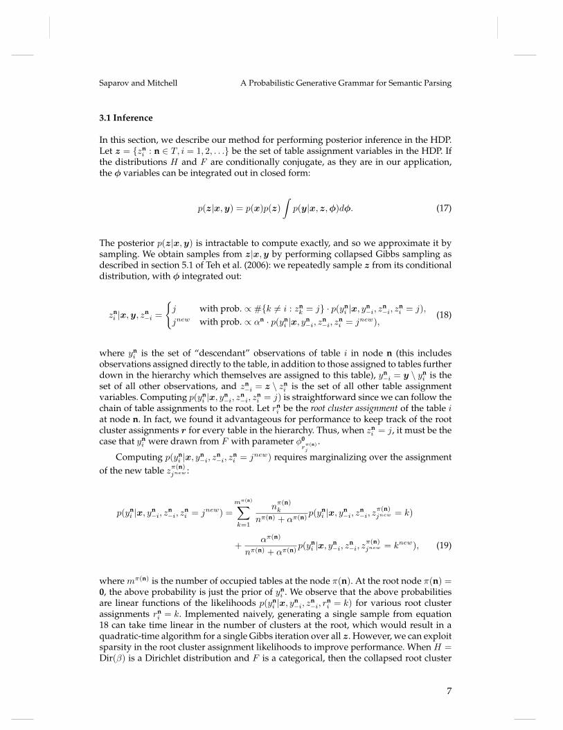
3.1 Inference
In this section, we describe our method for performing posterior inference in the HDP.Let z = {zn
i : n ∈ T, i = 1, 2, . . .} be the set of table assignment variables in the HDP. Ifthe distributions H and F are conditionally conjugate, as they are in our application,the φ variables can be integrated out in closed form:
p(z|x,y) = p(x)p(z)
∫p(y|x, z,φ)dφ. (17)
The posterior p(z|x,y) is intractable to compute exactly, and so we approximate it bysampling. We obtain samples from z|x,y by performing collapsed Gibbs sampling asdescribed in section 5.1 of Teh et al. (2006): we repeatedly sample z from its conditionaldistribution, with φ integrated out:
zni |x,y, zn
−i =
{j with prob. ∝ #{k 6= i : zn
k = j} · p(yni |x, yn
−i, zn−i, z
ni = j),
jnew with prob. ∝ αn · p(yni |x, yn
−i, zn−i, z
ni = jnew),
(18)
where yni is the set of “descendant” observations of table i in node n (this includes
observations assigned directly to the table, in addition to those assigned to tables furtherdown in the hierarchy which themselves are assigned to this table), yn
−i = y \ yni is the
set of all other observations, and zn−i = z \ zn
i is the set of all other table assignmentvariables. Computing p(yn
i |x, yn−i, z
n−i, z
ni = j) is straightforward since we can follow the
chain of table assignments to the root. Let rni be the root cluster assignment of the table i
at node n. In fact, we found it advantageous for performance to keep track of the rootcluster assignments r for every table in the hierarchy. Thus, when zn
i = j, it must be thecase that yn
i were drawn from F with parameter φ0rπ(n)j
.
Computing p(yni |x, yn
−i, zn−i, z
ni = jnew) requires marginalizing over the assignment
of the new table zπ(n)jnew :
p(yni |x, yn
−i, zn−i, z
ni = jnew) =
mπ(n)∑k=1
nπ(n)k
nπ(n) + απ(n)p(yn
i |x, yn−i, z
n−i, z
π(n)jnew = k)
+απ(n)
nπ(n) + απ(n)p(yn
i |x, yn−i, z
n−i, z
π(n)jnew = knew), (19)
where mπ(n) is the number of occupied tables at the node π(n). At the root node π(n) =0, the above probability is just the prior of yn
i . We observe that the above probabilitiesare linear functions of the likelihoods p(yn
i |x, yn−i, z
n−i, r
ni = k) for various root cluster
assignments rni = k. Implemented naively, generating a single sample from equation
18 can take time linear in the number of clusters at the root, which would result in aquadratic-time algorithm for a single Gibbs iteration over all z. However, we can exploitsparsity in the root cluster assignment likelihoods to improve performance. When H =Dir(β) is a Dirichlet distribution and F is a categorical, then the collapsed root cluster
7

Computational Linguistics Volume xx, Number xx
assignment likelihood is:
p(yni |x, yn
−i, zn−i, r
ni = k) =
∏t
(βt +#{t ∈ y0
k})(#{t∈yn
i })(∑t βt +#y0
k
)(#yni )
. (20)
Here, a(b) is the rising factorial a(a+ 1)(a+ 2) . . . (a+ b− 1) = Γ(a+b)Γ(a) , and #{t ∈ yn
i } isthe number of elements in yn
i with value t. Notice that the denominator depends onlyon the sizes and not on the contents of yn
i and y0k. Caching the denominator values for
common sizes of yni and y0
k can allow the sampler to avoid needless recomputation.This is especially useful in our application since many of the tables at the root tend to besmall. Similarly, observe that the numerator factor is 1 for values of twhere #{t ∈ yn
i } =0. Thus, the time required to compute the above probability is linear in the number ofunique elements of yn
i , which can improve the scalability of our sampler. We performthe above computations in log space to avoid numerical overflow.
3.1.1 Computing probabilities of paths. In previous uses of the HDP, the paths xiare assumed to be fixed. For instance, in document modeling, the paths correspondto documents or predefined categories of documents. In our application, however, thepaths may be random. In fact, we will later show that our parser heavily relies on theposterior predictive distribution over paths, where the paths correspond to semanticparses. More precisely, given a collection of training observations y = {y1, . . . , yn}withtheir paths x = {x1, . . . , xn}, we want to compute the probability of a new path xnew
given a new observation ynew:
p(xnew|ynew,x,y) ∝ p(xnew)∫p(ynew|z, xnew)p(z|x,y)dz, (21)
≈ p(xnew)
Nsamples
∑z∗∼z|x,y
p(ynew|z∗, xnew). (22)
Once we have the posterior samples z∗, we can compute the quantity p(ynew|z∗, xnew)by marginalizing over the table assignment for the new observation y:
p(ynew|z∗, xnew) =mx
new∑j=1
nxnew
j
nxnew + αxnewp(ynew|z∗, θnew = φx
new
j )
+αx
new
nxnew + αxnewp(ynew|z∗, θnew = φx
new
jnew ). (23)
Here, mxnew is the number of occupied tables at node xnew, nxnew
j is the number ofcustomers sitting at table j at node xnew, and nx
newis the total number of customers at
node xnew. The first term p(ynew|z∗, θnew = φxnew
j ) can be computed since the jth tableexists and is assigned to a table in its parent node, which in turn is assigned to a tablein its parent node, and so on. We can follow the chain of table assignments to the root.In the second term, the observation is assigned to a new table, whose assignment isunknown, and so we marginalize again over the assignment in the parent node for this
8
Saparov and Mitchell A Probabilistic Generative Grammar for Semantic Parsing
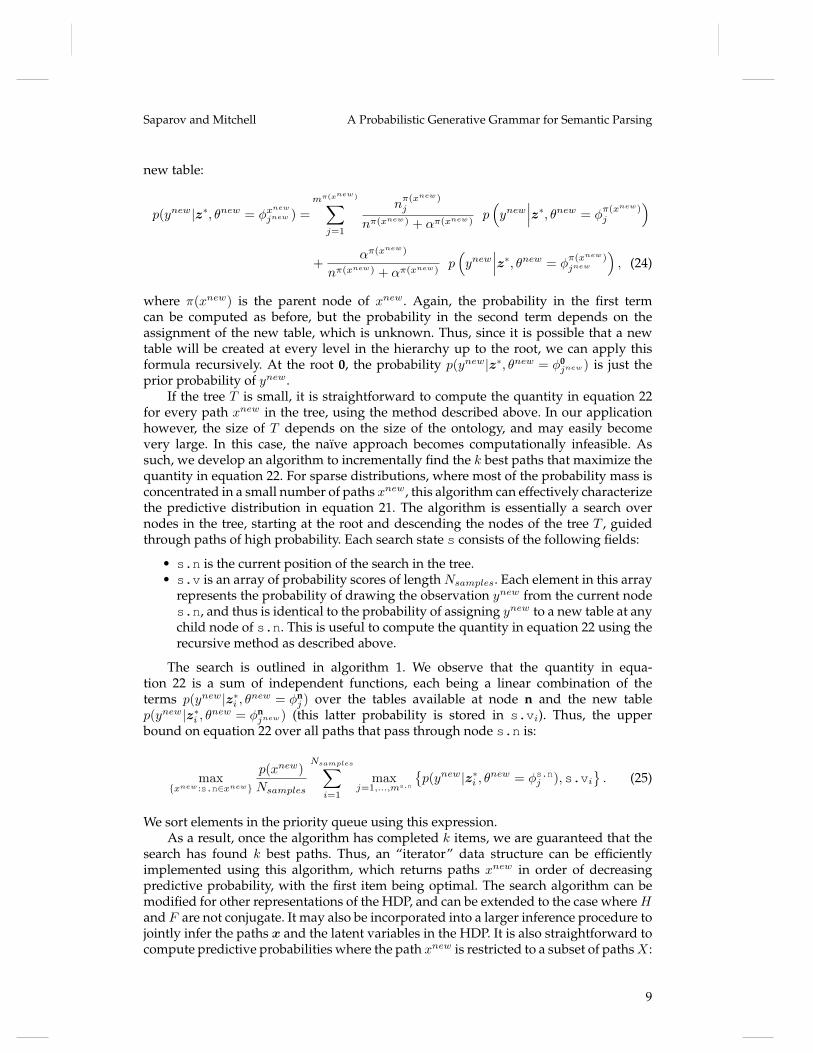
new table:
p(ynew|z∗, θnew = φxnew
jnew ) =
mπ(xnew)∑j=1
nπ(xnew)j
nπ(xnew) + απ(xnew)p(ynew
∣∣∣z∗, θnew = φπ(xnew)j
)
+απ(xnew)
nπ(xnew) + απ(xnew)p(ynew
∣∣∣z∗, θnew = φπ(xnew)jnew
), (24)
where π(xnew) is the parent node of xnew. Again, the probability in the first termcan be computed as before, but the probability in the second term depends on theassignment of the new table, which is unknown. Thus, since it is possible that a newtable will be created at every level in the hierarchy up to the root, we can apply thisformula recursively. At the root 0, the probability p(ynew|z∗, θnew = φ0
jnew) is just theprior probability of ynew.
If the tree T is small, it is straightforward to compute the quantity in equation 22for every path xnew in the tree, using the method described above. In our applicationhowever, the size of T depends on the size of the ontology, and may easily becomevery large. In this case, the naïve approach becomes computationally infeasible. Assuch, we develop an algorithm to incrementally find the k best paths that maximize thequantity in equation 22. For sparse distributions, where most of the probability mass isconcentrated in a small number of paths xnew, this algorithm can effectively characterizethe predictive distribution in equation 21. The algorithm is essentially a search overnodes in the tree, starting at the root and descending the nodes of the tree T , guidedthrough paths of high probability. Each search state s consists of the following fields:
• s.n is the current position of the search in the tree.• s.v is an array of probability scores of length Nsamples. Each element in this array
represents the probability of drawing the observation ynew from the current nodes.n, and thus is identical to the probability of assigning ynew to a new table at anychild node of s.n. This is useful to compute the quantity in equation 22 using therecursive method as described above.
The search is outlined in algorithm 1. We observe that the quantity in equa-tion 22 is a sum of independent functions, each being a linear combination of theterms p(ynew|z∗i , θnew = φn
j ) over the tables available at node n and the new tablep(ynew|z∗i , θnew = φn
jnew) (this latter probability is stored in s.vi). Thus, the upperbound on equation 22 over all paths that pass through node s.n is:
max{xnew:s.n∈xnew}
p(xnew)
Nsamples
Nsamples∑i=1
maxj=1,...,ms.n
{p(ynew|z∗i , θnew = φs.nj ),s.vi
}. (25)
We sort elements in the priority queue using this expression.As a result, once the algorithm has completed k items, we are guaranteed that the
search has found k best paths. Thus, an “iterator” data structure can be efficientlyimplemented using this algorithm, which returns paths xnew in order of decreasingpredictive probability, with the first item being optimal. The search algorithm can bemodified for other representations of the HDP, and can be extended to the case whereHand F are not conjugate. It may also be incorporated into a larger inference procedure tojointly infer the paths x and the latent variables in the HDP. It is also straightforward tocompute predictive probabilities where the path xnew is restricted to a subset of pathsX :
9

Computational Linguistics Volume xx, Number xx
Algorithm 1: Search algorithm to find the k best paths in the HDP that maximizethe quantity in equation 22.
1 initialize priority queue with initial state s2 s.n← 0 /* start at the root */3 for i = 1, . . . , Nsamples, do
4 s.vi ←∑m0
j=1
n0j
n0+α0 p(ynew|z∗i , θnew = φ0
j) +α0
n0+α0 p(ynew|z∗i , θnew = φ0
jnew)
5 repeat6 pop state s from the priority queue7 if s.n is a leaf8 complete the path s.n with probability p{xnew=s.n}
Nsamples
∑Nsamplesi=1 s.vi
9 foreach child node c of s.n, do10 create new search state s∗
11 s∗.n← c12 for i = 1, . . . , Nsamples, do13 s∗.vi ←
∑mc
j=1
ncj
nc+αc p(ynew|z∗i , θnew = φc
j) +αc
nc+αcs.vi
14 push s∗ onto priority queue with key in equation 25
15 until there are k completed paths
p(xnew|ynew,x,y, xnew ∈ X). To do so, the algorithm is restricted to only expand nodesthat belong to paths in X .
An important concern when performing inference with very large trees T is thatit is not feasible to explicitly store every node in memory. Fortunately, collapsed Gibbssampling does not require storing nodes whose descendants have zero observations. Inaddition, algorithm 1 can be augmented to avoid storing these nodes, as well. To doso, we make the observation that for any node n ∈ T in the tree whose descendantshave no observations, n will have zero occupied tables. Therefore, the probabilityp(ynew|z∗, xnew) = p(ynew|z∗, θnew = φn
jnew) is identical for any path xnew that passesthrough n. Thus, when the search reaches node n, it can simultaneously complete allpaths xnew that pass through n, and avoid expanding nodes with zero observationsamong its descendants. As a result, we only need to explicitly store a number of nodeslinear in the size of the training data, which enables practical inference with very largehierarchies.
There is a caveat that arises when we wish to compute a joint predictive probabilityp(xnew1 , . . . , xnewk |ynew1 , . . . , ynewk ,x,y), where we have multiple novel observations. Re-writing equation 21 in this setting, we have:
p(xnew1 , . . . , xnewk |ynew1 , . . . , ynewk ,x,y)
∝ p(xnew)∫p(ynew1 , . . . , ynewk |z∗,xnew)p(z|x,y)dz. (26)
For the CRF, the joint likelihood p(ynew1 , . . . , ynewk |z∗,xnew) does not factorize, since theobservations are not independent (they are exchangeable). One workaround is to usea representation of the HDP where the joint likelihood factorizes, such as the directassignment representation (Teh et al. 2006). Another approach is to approximate the
10

Saparov and Mitchell A Probabilistic Generative Grammar for Semantic Parsing
joint likelihood with the factorized likelihood. In our parser, we instead make thefollowing approximation:
p(ynew1 , . . . , ynewk |xnew,x,y) =k∏i=1
p(ynewi |ynew1 , . . . , ynewi−1 ,xnew,x,y) (27)
≈k∏i=1
p(ynewi |xnew,x,y). (28)
Substituting into equation 26, we obtain:
p(xnew|ynew,x,y) ∝ p(xnew)k∏i=1
∫p(ynewi |z∗,xnew)p(z|x,y)dz. (29)
When the size of the training data (x,y) is large with respect to the test data(xnew,ynew), the approximation works well, which we also find to be the case in ourexperiments.
4. Generative semantic grammar
We present a generative model of text sentences. In this model, semantic statementsare generated probabilistically from some higher-order process. Given each semanticstatement, a formal grammar selects text phrases, which are concatenated to form theoutput sentence. We present the model such that it remains flexible with regard to the se-mantic formalism. Even though our grammar can be viewed as an extension of context-free grammars, it is important to note that our model of grammar is only conditionallycontext-free, given the semantic statement. Otherwise, if the semantic information ismarginalized out, the grammar is sensitive to context.
4.1 Definition
Let N be a set of nonterminals, and let W be a set of terminals. Let R be a set ofproduction rules which can be written in the form A→ B1 . . .Bk where A ∈ N andB1, . . . ,Bk ∈ W ∪ N . The tuple (W,N ,R) is a context-free grammar (CFG) (Chomsky1956).
We couple syntax with semantics by augmenting the production rules R. In everyproduction rule A→ B1 . . .Bk in R, we assign to every right-hand side symbol Bi asurjective operation fi : XA 7→ XBi that transforms semantic statements, whereXA is theset of semantic statements associated with the symbol A and XBi is the set of semanticstatements associated with the symbol Bi. Intuitively, the operation describes how thesemantic statement is “passed on” to the child nonterminals in the generative pro-cess. During parsing, these operations will describe how simpler semantic statementscombine to form larger statements, enabling semantic compositionality. For example,suppose we have a semantic statement x = has_color(reptile:frog,color:green) and the pro-duction rule S→ NP VP. We can pair the semantic operation f1 with the NP in theright-hand side such that f1(x) = reptile:frog selects the subject argument. Similarly, wecan pair the semantic operation f2 with the VP in the right-hand side such that f2(x) = xis the identity operation. The augmented production rule is (A,B1, . . . ,Bk, f1, . . . , fk)
11

Computational Linguistics Volume xx, Number xx
and the set of augmented rules is R∗. In parsing, we require the computation of theinverse of semantic operations, which is the preimage of a given semantic statementf−1(x) = {x′ : f(x′) = x}. Continuing the example above, f−1
1 (reptile:frog) returns a setthat contains the statement has_color(reptile:frog,color:green) in addition to statements likeeats_insect(reptile:frog,insect:fly).
To complete the definition of our grammar, we need to specify the method that,given a nonterminal A ∈ N and a semantic statement x ∈ XA, selects a production rulefrom the set of rules in R∗ with the left-hand side nonterminal A. To accomplish this,we define selectA,x as a distribution over rules from R∗ that has A as its left-handside, dependent on x. We will later provide a number of example definitions of thisselectA,x distribution. Thus, a grammar in our framework is fully specified by thetuple (W,N ,R∗,select).
Note that other semantic grammar formalisms can be fit into this framework. Forexample, in categorical grammars, a lexicon describes the mapping from elementarycomponents of language (such as words) to a syntactic category and a semantic mean-ing. Rules of inference are available to combine these lexical items into (tree-structured)derivations, eventually resulting in a syntactic and semantic interpretation of the fullsentence (Steedman 1996; Jäger 2004). In our framework, we imagine this process inreverse. The setXS is the set of all derivable semantic statements with syntactic categoryS. The generative process begins by selecting one statement from this set x ∈ XS .Next, we consider all applications of the rules of inference that would yield x, witheach unique application of an inference rule being equivalent to a production rule inour framework. We select one of these production rules according to our generativeprocess and continue recursively. The items in the lexicon are equivalent to preterminalproduction rules in our framework. Thus, the generative process below describes a wayto endow parses in categorical grammar with a probability measure. This can be used,for example, to extend earlier work on generative models with CCG (Hockenmaier 2001;Hockenmaier and Steedman 2002). Different choices of the select distribution inducedifferent probability distributions over parses.
We do not see a straightforward way to fit linear or log-linear models over fullparses into our framework, where a vector of features can be computed for each fullparse (Berger, Pietra, and Pietra 1996; Ratnaparkhi 1998). This is due to our assumptionthat, given the semantic statement, the probability of a parse factorizes over the pro-duction rules used to construct that parse. However, the select distribution can bedefined using linear and log-linear models, as we will describe in section 4.3.
12
Saparov and Mitchell A Probabilistic Generative Grammar for Semantic Parsing
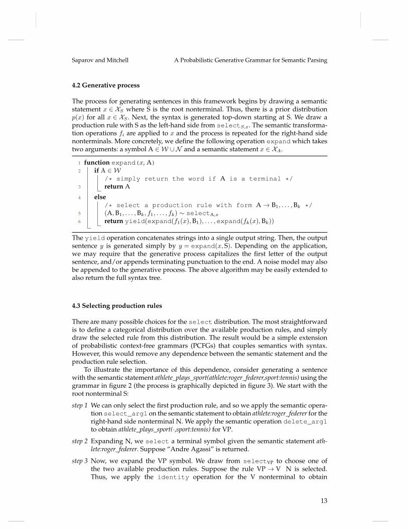
4.2 Generative process
The process for generating sentences in this framework begins by drawing a semanticstatement x ∈ XS where S is the root nonterminal. Thus, there is a prior distributionp(x) for all x ∈ XS . Next, the syntax is generated top-down starting at S. We draw aproduction rule with S as the left-hand side from selectS,x. The semantic transforma-tion operations fi are applied to x and the process is repeated for the right-hand sidenonterminals. More concretely, we define the following operation expand which takestwo arguments: a symbol A ∈ W ∪N and a semantic statement x ∈ XA.
1 function expand(x, A)2 if A ∈ W
/* simply return the word if A is a terminal */3 return A
4 else/* select a production rule with form A→ B1, . . . ,Bk */
5 (A,B1, . . . ,Bk, f1, . . . , fk) ∼ selectA,x6 return yield(expand(f1(x),B1), . . . ,expand(fk(x),Bk))
The yield operation concatenates strings into a single output string. Then, the outputsentence y is generated simply by y = expand(x, S). Depending on the application,we may require that the generative process capitalizes the first letter of the outputsentence, and/or appends terminating punctuation to the end. A noise model may alsobe appended to the generative process. The above algorithm may be easily extended toalso return the full syntax tree.
4.3 Selecting production rules
There are many possible choices for the select distribution. The most straightforwardis to define a categorical distribution over the available production rules, and simplydraw the selected rule from this distribution. The result would be a simple extensionof probabilistic context-free grammars (PCFGs) that couples semantics with syntax.However, this would remove any dependence between the semantic statement and theproduction rule selection.
To illustrate the importance of this dependence, consider generating a sentencewith the semantic statement athlete_plays_sport(athlete:roger_federer,sport:tennis) using thegrammar in figure 2 (the process is graphically depicted in figure 3). We start with theroot nonterminal S:
step 1 We can only select the first production rule, and so we apply the semantic opera-tion select_arg1 on the semantic statement to obtain athlete:roger_federer for theright-hand side nonterminal N. We apply the semantic operation delete_arg1to obtain athlete_plays_sport(·,sport:tennis) for VP.
step 2 Expanding N, we select a terminal symbol given the semantic statement ath-lete:roger_federer. Suppose “Andre Agassi” is returned.
step 3 Now, we expand the VP symbol. We draw from selectVP to choose one ofthe two available production rules. Suppose the rule VP→ V N is selected.Thus, we apply the identity operation for the V nonterminal to obtain
13

Computational Linguistics Volume xx, Number xx
S→ N : select_arg1 VP : delete_arg1 N→ “tennis”VP→ V : identity N : select_arg2 N→ “Andre Agassi”VP→ V : identity N→ “Chopin”
V→ “swims”V→ “plays”
Figure 2Example of a grammar in our framework. This grammar operates on semantic statements of theform predicate(first argument, second argument). The semantic operation select_arg1 returns thefirst argument of the semantic statement. Likewise, the operation select_arg2 returns thesecond argument. The operation delete_arg1 removes the first argument, and identityreturns the semantic statement with no change.
athlete_plays_sport(·,sport:tennis). We similarly apply select_arg2 for the Nnonterminal to obtain sport:tennis.
step 4 We expand the V nonterminal, drawing from selectV on the semantic statementathlete_plays_sport(·,sport:tennis). Suppose “plays” is returned.
step 5 Finally, we expand the N nonterminal, drawing from selectN with the state-ment sport:tennis. Suppose “tennis” is returned. We concatenate all returnedstrings to form the sentence “Andre Agassi plays tennis.”
However, now consider generating another sentence with the same grammar for thestatement athlete_plays_sport(athlete:roger_federer, sport:swimming). In step 3 of the aboveprocess, the select distribution would necessarily have to depend on the seman-tic statement. In English, the probability of observing a sentence of the form N V N(’Rachmaninoff makes music’) versus N V (’Rachmaninoff composes’) depends on theunderlying semantic statement.
To capture this dependence, we use HDPs to define the select distribution. Everynonterminal A ∈ N is associated with an HDP, and in order to fully specify the gram-mar, we need to specify the structure of each HDP tree. Let TA be the tree associatedwith the nonterminal A. The model is flexible with how the trees are defined, but weconstruct trees with the following method. First, select m discrete features g1, . . . , gmwhere each gi : X 7→ Z and Z is the set of integers. These features operate on semanticstatements. For example, suppose we restrict the space of semantic statements to be theset of single predicate instances (triples). The relations in an ontology can be assignedunique integer indices, and so we may define a semantic feature as a function whichsimply returns the index of the predicate given a semantic statement. We construct theHDP tree TA starting with the root, we add a child node for every possible output of g1.We repeat the process recursively, constructing a complete tree of depth m+ 1.
As an example, we will construct a tree for the nonterminal VP for the examplegrammar in figure 2. Suppose in our ontology, we have the predicates athlete_plays_sportand musician_plays_instrument, labeled 0 and 1, respectively. The ontology also containsthe concepts athlete:roger_federer, sport:tennis, and sport:swimming, also labeled 0, 1, and2, respectively. We define the first feature g1 to return the predicate index. The secondfeature g2 returns the index of the concept in the second argument of the semanticstatement. The tree is constructed starting with the root, we add a child node foreach predicate in the ontology: athlete_plays_sport and musician_plays_instrument. Next,for each child node, we add a grandchild node for every concept in the ontology:athlete:roger_federer, sport:tennis, and sport:swimming. The resulting tree TV P has depth
14

Saparov and Mitchell A Probabilistic Generative Grammar for Semantic Parsing
step 0:
S
athlete_plays_sport(athlete:roger_federer,sport:tennis)
step 1:
S
N VP
athlete:roger_federer athlete_plays_sport(·, sport:tennis)
step 2:
S
N
“Roger Federer”
VP
athlete_plays_sport(·, sport:tennis)
step 3:
S
N
“Roger Federer”
VP
V N
athlete_plays_sport(·, sport:tennis)
sport:tennis
step 4:
S
N
“Roger Federer”
VP
V
“plays”
N
sport:tennis
step 5:
S
N
“Roger Federer”
VP
V
“plays”
N
“tennis.”
Figure 3A depiction of the generative process producing a sentence for the semantic statementathlete_plays_sport(athlete:roger_federer,sport:tennis) using the grammar in figure 2.
2, with a root node with 2 child nodes, and each child node has 3 grandchild nodes.This construction enables the select distribution for the nonterminal VP to depend onthe predicate and the second argument of the semantic statement.
With the fully-specified HDPs and their corresponding trees, we have fully specifiedselect. When sampling from selectA,x for the nonterminal A ∈ N and a semanticstatement x ∈ X , we compute them semantic features for the given semantic statement:g1(x), g2(x), . . . , gm(x). This sequence of indices specifies a path from the root of the tree
15

Computational Linguistics Volume xx, Number xx
down to a leaf. We then simply draw a production rule observation from this leaf node,and return the result: r ∼ HDP(x, TA) = selectA,x.
There are many other alternatives for defining the select distribution. For in-stance, a log-linear model can be used to learn dependence on a set of features. TheHDP provides statistical advantages, smoothing the learned distributions, resulting ina model more robust to data sparsity issues.
In order to describe inference in this framework, we must define additional conceptsand notation. For a nonterminal A ∈ N , observe that the paths from the root to theleaves of its HDP tree induce a partition on the set of semantic statements XA. Moreprecisely, two semantic statements x1, x2 ∈ XA belong to the same equivalence class ifthey correspond to the same path in an HDP tree.
S
NP
N
VP
V NP
N
PP
P N
full parse
=
S
NP
N
VP
V
left outer parse
+ NP
N
innerparse
+ PP
P N
right outer parse
Figure 4An example decomposition of a parse tree into its left outer parse, inner parse (of the object nounphrase), and its right outer parse. This is one example of such a decomposition. For instance, wemay similarly produce a decomposition where the prepositional phrase is the inner parse, orwhere the verb is the inner parse. The terminals are omitted and only the syntactic portion of theparse is displayed here for consiseness.
Every parse (x, s) consists of a semantic statement x and a syntax tree s. The syntaxtree s is a rooted tree containing an interior vertex for every nonterminal and a leaf forevery terminal. Every vertex is associated with a start position and end position in thesentence. An interior vertex along with its immediate children corresponds to a par-ticular production rule in the grammar (A→ B1:f1 . . .Bn:fn) ∈ R∗, where the interiorvertex is associated with the nonterminal A and its children respectively correspondto the symbols B1, . . . ,Bn, left-to-right. Thus, every edge in the tree is labeled with asemantic transformation operation. A subgraph sI of s can be called an inner syntax tree.The corresponding outer syntax tree sO is sO = s \ sI is the syntax tree with sI deleted.We further draw a distinction between left and right components of an outer syntaxtree. Define the left outer syntax tree sL as the minimal subgraph of sO containing allsubtrees positioned to the left of sI , and containing all ancestor vertices of sI . The rightouter syntax tree sR forms the remainder of the outer parse, and so s can be decomposedinto three distinct trees: s = sL ∪ sR ∪ sI . See figure 4 for an illustration. Note that itis possible that sR consists of multiple disconnected trees. In the description of ourparser, we will frequently use the notation p(s) to refer to the joint probability of allthe production rules in the syntax tree s; that is, p(s) = p(
⋂(A→β)∈s A→ β), where β is
the right-hand side of some production rule.
16

Saparov and Mitchell A Probabilistic Generative Grammar for Semantic Parsing
5. Inference
Let y , {y1, . . . , yn} be a collection of training sentences, along with their correspondingsyntax trees s , {s1, . . . , sn} and semantic statement labels x , {x1, . . . , xn}. Given anew sentence ynew, the goal of parsing is to compute the probability of its semanticstatement xnew and syntax snew:
p(xnew, snew|ynew,x, s,y) ∝∫p(xnew, snew, ynew|θ)p(θ|x, s,y)dθ. (30)
In this expression, θ are the latent variables in the grammar. Different applicationswill rely on this probability in different ways. For example, we may be interested inthe semantic parse that maximizes this probability. The above integral is intractable tocompute exactly, so we use Markov chain Monte Carlo (MCMC) to approximate it:
≈ 1
Nsamples
∑θ∗∼θ|x,s,y
p(xnew, snew, ynew|θ∗), (31)
where the sum is taken over samples from the posterior of the latent grammar variablesθ given the training data x, s, and y.1
We make the assumption that the likelihood factorizes over the nonterminals. Moreprecisely:
p(ynew, snew|xnew,θ) =∏A∈N
p({A→ β ∈ snew}|xnew, θA), (32)
where θA are the latent variables specific to the nonterminal A, and {A→ β ∈ snew} isthe set of production rules in snew that have A as the left-hand side nonterminal. Thus,we may factorize the joint likelihood as:
p(xnew, snew, ynew|θ) = p(xnew)∏
A∈N
p ({A→ β ∈ snew}|xnew, θA) , (33)
where the first product is over the nonterminals A ∈ N in the grammar. Note thatthe probability p (A→ β|xnew, θA) is equivalent to the probability of drawing the ruleA→ β from selectA,xnew for nonterminal A and semantic statement xnew. Plugging
1 We also attempted a variational approach to inference, approximating the integral asEq [p(x
new, snew, ynew|θ)], where q was selected to minimize the KL divergence to the posteriorp(θ|x,s,y). We experimented with a number of variational families, but we found that they were notsufficiently expressive to accurately approximate the posterior for our purposes.
17

Computational Linguistics Volume xx, Number xx
equation 33 into 30 and 31, we obtain:
p(xnew, snew|ynew,x, s,y)
∝ p(xnew)∏
A∈N
∫p ({A→ β ∈ snew}|xnew, θA) p(θA|x, s,y)dθA, (34)
≈ p(xnew)
N|N |samples
∏A∈N
∏(A→β)∈snew
∑θ∗A∼θA|x,s,y
p (A→ β|xnew, θ∗A) , (35)
where the second product iterates over the production rules that constitute the syntaxsnew. Note that we applied the approximation as described in equation 28. The semanticprior p(xnew) plays a critically important role in our framework. It is through this priorthat we can add dependence on background knowledge during parsing. Although wepresent a setting in which training is supervised with both syntax trees and semanticlabels, it is straightforward to apply our model in the setting where we have semanticlabels but syntax information is missing. In such a setting, a Gibbs step can be addedwhere the parser is run on the input sentence with the fixed semantic statement, return-ing a distribution over syntax trees for each sentence.
Now, we divide the problem of inference into two major components:
Inference over HDP paths: Given a set of semantic statements X ⊆ X , incrementallyfind the k best semantic statements x ∈ X that maximize the sum
∑p(A→
β|x, θA) within equation 35. We observe that this quantity only depends on theHDP associated with nonterminal A. Note that this is exactly the setting as de-scribed in section 3.1.1, and so we can directly apply algorithm 1 to implementthis component.
Parsing: Efficiently compute the k most likely semantic and syntactic parses{xnew, snew} that maximize p(xnew, snew|ynew,x, s,y) for a given sentence ynew.We describe this component in greater detail in the next section. This componentutilizes the previous component.
5.1 Parsing
We develop a top-down parsing algorithm that computes the k-best semantic/syntacticparses (xnew, snew) that maximize p(xnew, snew|ynew,x, s,y) for a given sentence ynew.We emphasize that this parser is largely independent of the choice of the distributionselect. The algorithm searches over a space of items called rule states, where eachrule state represents the parser’s position within a specific production rule of thegrammar. Complete rule states represent the parser’s position after completing parsingof a rule in the grammar. The algorithm also works with nonterminal structures thatrepresent a completed parse of a nonterminal within the grammar. The parser keepsa priority queue of unvisited rule states called the agenda. A data structure called thechart keeps intermediate results on contiguous portions of the sentence. A predefinedset of operations are available to the algorithm. At every iteration of the main loop, thealgorithm pops the rule state with the highest weight from the agenda and adds it to thechart, applying any available operation on this state using any intermediate structuresin the chart. These operations may add additional rule states to the agenda, with prioritygiven by an upper bound on log p(xnew, snew|ynew,x, s,y). The overall structure of ourparser is reminiscent of the Earley parsing algorithm, which is the classical example of
18

Saparov and Mitchell A Probabilistic Generative Grammar for Semantic Parsing
a top-down parsing algorithm for CFGs (Earley 1970). We will draw similarities in ourdescription below. The parsing procedure can also be interpreted as an A∗ search over alarge hypergraph.
Each rule state r is characterized by the following fields:
. rule is the production rule currently being parsed.
. start is the (inclusive) sentence position marking the beginning of the produc-tion rule.
. end is the (exclusive) sentence position marking the end of the production rule.
. i is the current position in the sentence.
. k is the current position in the production rule. Dotted rule notation is a conve-nient way to represent the variables rule and k. For example, if the parser iscurrently examining the rule A→ B1 . . .Bn at rule position k (omitting seman-tic transformation operations), we may write this as A→ B1 . . .Bk • Bk+1 . . .Bnwhere the dot denotes the current position of the parser.
. semantics is a set of semantic statements.
. syntax is a partially completed syntax tree. As an example, if the parser iscurrently examining rule A→ B1 . . .Bn at position k, the tree will have a root nodelabeled A with k child subtrees each labeled B1 through Bk, respectively.
. log_probability is the inner log probability of the rule up to its current posi-tion.
Every complete rule state r contains the above fields in addition to an iterator fieldwhich keeps intermediate state for the inference method described in section 3.1.1 (seedescription of the iteration operation below for details on how this is used).Every nonterminal structure n contains the fields:
. start, end, semantics, syntax, and log_probability are identical to therespective fields in the rule states.
. nonterminal is the nonterminal currently being parsed.
The following are the available operations or deductions that the parser can performwhile processing rule states:
expansion takes an incomplete rule state r as input. For notational convenience, letk = r.k and r.rule be written as A→ B1 . . .Bn. This operation examines thenext right-hand symbol Bk. There are two possible cases:
If Bk is a nonterminal: For every production rule in the grammar Bk → β whoseleft-hand symbol is Bk, for every j ∈ {r.i, . . . ,r.end}, create a new rule state r∗
only if Bk was not previously expanded at this given start and end position:r∗.rule = Bk → β, r∗.start = r.i, r∗.end = j,r∗.i = r.i, r∗.k = 0, r∗.log_probability = 0.
The semantic statement field of the new state is set to be the set of all semanticstatements for the expanded nonterminal: r∗.semantics = XBk . The syntax treeof the new rule state r∗.syntax is initialized as a single root node. The new rulestate is added to the agenda (we address specifics on prioritization later). Thisoperation is analogous to the “prediction” step in Earley parsing.
19

Computational Linguistics Volume xx, Number xx
If Bk is a terminal: Read the terminal Bk in the sentence starting at position r.i,then create a new rule state r∗ where:r∗.rule = r.rule, r∗.start = r.start, r∗.end = r.end,r∗.i = r.i+ |Bk|, r∗.k = r.k+ 1,r∗.log_probability = r.log_probability,r∗.semantics = r.semantics.
The new syntax tree is identical to the old syntax tree with an added child nodecorresponding to this terminal symbol Bk. The new rule state is then added to theagenda. This operation is analogous to the “scanning” step in Earley parsing.
completion takes as input an incomplete rule state r, and a nonterminal structure nwhere n.nonterminalmatches the next right-hand nonterminal in r.rule, andwhere the starting position of the nonterminal structure n.start matches thecurrent sentence position of the rule state r.i. For notational convenience, letr.rule be written as A→ B1:f1 . . .Bn:fn. The operation constructs a new rulestate r∗:r∗.rule = r.rule, r∗.start = r.start, r∗.end = r.end,r∗.i = n.end, r∗.k = r.k+ 1.
To compute the semantic statements of the new rule state, first invert the se-mantic statements of the nonterminal structure n with the semantic transforma-tion operation f−1
k , and then intersect the resulting set with the semantic state-ments of the incomplete rule state: r∗.semantics = r.semantics ∩ {f−1
k (x) :x ∈ n.semantics}. The syntax tree of the new rule state r∗.syntax is the syntaxtree of the old incomplete rule state r.syntax with the added subtree of the non-terminal structure n.syntax. The log probability of the new rule state is the sumof that of both input states: r∗.log_probability = r.log_probability+n.log_probability. The new rule state r∗ is then added to the agenda. Thisoperation is analogous to the “completion” step in Earley parsing.
iteration takes as input a complete rule state r. Having completed parsing the pro-duction rule r.rule = A→ β, we need to compute
∑θ∗Ap(A→ β|xnew, θ∗A) as in
equation 35. To do so, we determine HDP paths in order from highest to lowestposterior predictive probability using the HDP inference approach described insection 3.1.1. We store our current position in the list as r.iterator. This oper-ation increments the iterator and adds the rule state back into the agenda (if theiterator has a successive element). Next, this operation creates a new nonterminalstructure n∗ where:n∗.nonterminal = A, n∗.start = r.start,n∗.end = r.end, n∗.syntax = r.syntax.Recall that the paths in an HDP induce a partition of the set of semantic statementsXA, and so the path returned by the iterator corresponds to a subset of seman-tic statements X ⊆ XA. The semantic statements of the nonterminal structure iscomputed as the intersection of this subset with semantic statements of the rulestate: n∗.semantics = X ∩ r.semantics. The log probability of the new non-terminal structure n∗.log_probability is the sum of the log probability of thepath returned by the iterator and r.log_probability. The new nonterminalstructure is added to the chart.
The algorithm is started by executing the expansion operation on all production rulesof the form S→ β where S is the root nonterminal, starting at position 0 in the sen-tence, with semantics initialized as the set of all possible semantic statements XS .
20

Saparov and Mitchell A Probabilistic Generative Grammar for Semantic Parsing
To describe the prioritization of agenda items, recall that any complete syntax trees can be decomposed into inner, left outer, and right outer portions: s = sL ∪ sR ∪sI . Observe that the probability of the full parse (equation 35) can be written as aproduct of four terms: (1) the semantic prior p(xnew), (2) the left outer probabilityp(sL|xnew,x, s,y), (3) the right outer probability p(sR|xnew,x, s,y), and (4) the innerprobability p(sI |xnew,x, s,y).
Items in the agenda are sorted by an upper bound on the log probability of the entireparse. In order to compute this, we rely on an upper bound on the inner probability thatonly considers the syntactic structure:
IA,i,j , maxA→B1...Bn
(maxx′
log p(A→ B1 . . .Bn|x′,x, s,y) + maxm2≤...≤mn
n∑k=1
IBk,mk,mk+1
),
(36)where m1 = i and mn+1 = j. In the sum, if Bk is a terminal, then IBk,mk,mk+1
= 0 ifmk+1 −mk = |Bk| is the correct length of the terminal; otherwise IBk,mk,mk+1
= −∞.The term maxx′ log p(A→ B1 . . .Bn|x′,x, s,y) can be computed exactly using algorithm1, but a tight upper bound can be computed more quickly by terminating algorithm 1early and using the priority value given by equation 25 (we find that for preterminals,even using the priority computed at the root provides a very good estimate). The valueof I can be computed efficiently using existing syntactic (e.g., PCFG) parsers in timeO(n3).
We also compute an upper bound on the log probability of the outer portion of thesyntax tree and the semantic prior. To be more precise, let P(A, i, j) be the set of allparses (x, sL, sR, sI) such that s = sL ∪ sR ∪ sI is the syntax and sI is the inner syntaxtree with root A that begins at sentence position i (inclusive) and ends at j (exclusive).Then, a bound on the outer probability is:
OA,i,j , max(x,sL,sR,sI)∈P(A,i,j)
log p(x) + log p(sL|x,x, s,y) +∑
(A′,i′,j′)∈R(sR)
IA′,i′,j′ . (37)
where R(sR) is the set of root vertices of the trees contained in sR, and p(x) is the priorprobability of the semantic statement x ∈ XS . Note that the third term is an upper boundon the right outer probability p(sR|x, s,x,y).
Using these bounds, we can compute an upper bound on the overall log probabilityof the parse for any state. For a rule state r, the search priority is given by:
r.log_probability+ maxmk+1≤...≤mn
n∑l=k
IBl,ml,ml+1
+min {log p(r.semantics),OA,r.start,r.end} , (38)
where A→ B1 . . .Bk is the currently-considered rule r.rule, mk = r.i, and mn+1 =r.end. Note the first two terms constitute an upper bound on the inner probabilityof the nonterminal A, and the third term is an upper bound on the outer probabilityand semantic prior. The second term can be computed efficiently using dynamic pro-gramming. We further tighten this by adding a term that bounds the log probabilityof the rule log p(A→ B1 . . .Bk|x′,x, s,y). The items in the agenda are prioritized bythis quantity. As long as the log_probability field remains exact, as it does in ourapproach, the overall search will yield exact outputs. The use of a syntactic parser
21

Computational Linguistics Volume xx, Number xx
to compute a tigher bound on the outer probability in an A∗ parser is similar to theapproach of Klein and Manning (2003b).
Naive computation of equation 37 is highly infeasible, as it would require enumerat-ing all possible outer parses. However, we can rely on the fact that our search algorithmis monotonic: the highest score in the agenda never increases as the algorithm progresses.We prove monotonicity by induction on the number of iterations. For a given iteration i,by the inductive hypothesis, the parser has visited all reachable rule states with prioritystrictly larger than the priority of the current rule state. We will show that all new rulestates added to the priority queue at iteration i must have priority at most equal to thepriority of the current rule state. Consider each operation:
In the expansion operation, let i = r.i and k = r.k. If the next right-hand side symbolBk is a terminal, the new agenda item will have score at most that of the old agendaitem, since r∗.log_probability = r.log_probability and the sum of in-ner probability bounds in equation 38 cannot increase. If the Bk is a nonterminal,then we claim that any rule state created by this operation must have priority atmost the priority of the old agenda item. Suppose to the contrary that there existsa j ∈ {i, . . . ,r.end}, a rule Bk → C1 . . .Cu, and m′2 ≤ . . . ≤ m′u such that:
min{ log p(XBk),OBk,i,j}+u∑l=1
ICl,m′l,m′l+1
> r.log_probability+ maxmk+1≤...≤mn
n∑l=k
IBl,ml,ml+1
+min {log p(r.semantics),OA,r.start,r.end} ,
where mk = m′1 = i, m′u = j, and mn+1 = r.end. Note that the left-hand side isbounded above by IBk,i,j +OBk,i,j which implies, by the definition of OBk,i,j , thatthere exists a parse (x∗, s∗L, s
∗R, s
∗I) ∈ P(Bk, i, j) such that:
log p(x∗) + log p(s∗L|x∗,x, s,y) + IBk,i,j +∑
(A′,i′,j′)∈R(s∗R)
IA′,i′,j′
> r.log_probability+ maxmk+2≤...≤mn
n∑l=k
IBl,ml,ml+1
+min {log p(r.semantics),OA,r.start,r.end} ,
where mk+1 = j. Let C→ D1 . . .Dv be the production rule in the syntax tree s∗
containing s∗I . In addition, let s∗i be the sibling subtree of sI rooted at Di. Thisparse implies the existence of a rule state r∗ where r∗.rule = (C→ D1 . . .Dv),r∗.start and r∗.end are the start and end positions of the vertex correspondingto C, r∗.i = r.i, r∗.log_probability =
∑r∗.ki=1 log p(s∗i |x∗,x, s,y). The search
priority of this rule state would be:
r∗.k−1∑i=1
log p(s∗i |x∗,x, s,y) + maxmk+1≤...≤mv
v∑l=r∗.k
IDl,ml,ml+1
+min{log p(r∗.semantics),OC,r∗.start,r∗.end}
22
Saparov and Mitchell A Probabilistic Generative Grammar for Semantic Parsing
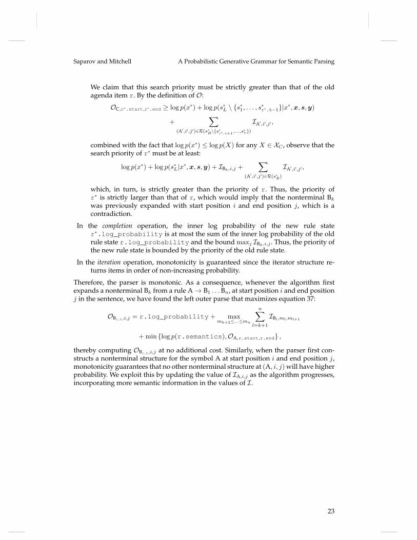
We claim that this search priority must be strictly greater than that of the oldagenda item r. By the definition of O:
OC,r∗.start,r∗.end ≥ log p(x∗) + log p(s∗L \ {s∗1, . . . , s∗r∗.k−1}|x∗,x, s,y)
+∑
(A′,i′,j′)∈R(s∗R\{s∗r∗.k+1,...,s∗v})
IA′,i′,j′ ,
combined with the fact that log p(x∗) ≤ log p(X) for any X ∈ XC , observe that thesearch priority of r∗ must be at least:
log p(x∗) + log p(s∗L|x∗,x, s,y) + IBk,i,j +∑
(A′,i′,j′)∈R(s∗R)
IA′,i′,j′ ,
which, in turn, is strictly greater than the priority of r. Thus, the priority ofr∗ is strictly larger than that of r, which would imply that the nonterminal Bkwas previously expanded with start position i and end position j, which is acontradiction.
In the completion operation, the inner log probability of the new rule stater∗.log_probability is at most the sum of the inner log probability of the oldrule state r.log_probability and the bound maxj IBk,i,j . Thus, the priority ofthe new rule state is bounded by the priority of the old rule state.
In the iteration operation, monotonicity is guaranteed since the iterator structure re-turns items in order of non-increasing probability.
Therefore, the parser is monotonic. As a consequence, whenever the algorithm firstexpands a nonterminal Bk from a rule A→ B1 . . .Bn, at start position i and end positionj in the sentence, we have found the left outer parse that maximizes equation 37:
OBr.k,i,j = r.log_probability+ maxmk+2≤...≤mn
n∑l=k+1
IBl,ml,ml+1
+min {log p(r.semantics),OA,r.start,r.end} ,
thereby computing OBr.k,i,j at no additional cost. Similarly, when the parser first con-structs a nonterminal structure for the symbol A at start position i and end position j,monotonicity guarantees that no other nonterminal structure at (A, i, j) will have higherprobability. We exploit this by updating the value of IA,i,j as the algorithm progresses,incorporating more semantic information in the values of I.
23

Computational Linguistics Volume xx, Number xx
Figure 5A step-by-step example of the parser running on the sentence “Chopin plays” using thegrammar very similar to the one shown in figure 2. The top-left table lists the semanticstatements sorted by their log probability of drawing the observation “Chopin” from the HDPassociated with the nonterminal N. The top-center and top-right tables are defined similarly.
N→ “Chopin” log prob.musician:chopin -2sport:swimming -8sport:tennis -8instrument:piano -8
* -8
The symbol * is a wildcard, re-ferring to any entity in the on-tology excluding those listed.
In this example, we use thegrammar in figure 2.
V→ “plays” log prob.athlete_plays_sport(*, *) -2musician_plays_inst(*, *) -2musician_plays_inst(*,
instrument:piano)-2
athlete_plays_sport(*,sport:tennis)
-2
athlete_plays_sport(*,sport:swimming)
-8
athlete_plays_sport(*,instrument:piano)
-8
......
VP→ V log prob.athlete_plays_sport(*, *) -4musician_plays_inst(*, *) -4athlete_plays_sport(*,
sport:swimming)-4
musician_plays_inst(*,instrument:piano)
-5
athlete_plays_sport(*,sport:tennis)
-5
athlete_plays_sport(*,instrument:piano)
-8
......
iteration operation new states created
0 expand S at start position0, end position 12
S→ • N VPi: 0, end: 12log_prob: 0
1
pop the S→ • N VP stateand expand N at start po-sition 0 and end positions0, . . . , 12
N→ “Chopin” •i: 6 , end: 6log_prob: 0
2 iterate the complete rulestate N→ “Chopin” •
Nstart: 0, end: 6log_prob: -2musician:chopin
3pop the N nonterminalstate and complete anywaiting rule states
S→ N • VPi: 7, end: 12log_prob: -2
* (musician:chopin, *)
4
pop the S→ N • VP stateand expand VP at start po-sition 7 and end position12
VP→ • Vi: 7, end: 12log_prob: 0
VP→ • V Ni: 7, end: 12log_prob: 0
VP→ • Vi: 7, end: 11log_prob: 0
. . .
5 pop the VP → • V stateand expand V
V→ “plays” •i: 12, end: 12log_prob: 0
6 iterate the complete rulestate V→ “plays” •
Vstart: 7, end: 12log_prob: -2
athlete_plays_sport(*, *)
Vstart: 7, end: 12log_prob: -2
musician_plays_inst(*, *)
. . .
7pop a V nonterminal stateand complete any waitingrule states
VP→ V •i: 12, end: 12log_prob: -2
musician_plays_inst(*, *)
VP→ V • Ni: 12, end: 12log_prob: -2
musician_plays_inst(*, *)
. . .
8 iterate the complete rulestate VP→ V •
VPstart: 7, end: 12log_prob: -6
musician_plays_inst(*, *)
9pop the VP nonterminalstate and complete anywaiting rule states
S→ N VP •i: 12, end: 12log_prob: -8
musician_plays_inst(musician:chopin, *)
24

Saparov and Mitchell A Probabilistic Generative Grammar for Semantic Parsing
S
N
Federer
VP
V
plays
N
tennis
simple grammar
athlete_plays_sport(athlete:roger_federer,sport:tennis)
S
N
Federer
VP
V
Vroot
play
Vaffix
s
N
tennis
verb morphology grammar
athlete_plays_sport(athlete:roger_federer,sport:tennis, time:present)
Figure 6An example of a (simpified) labeled data instance in our experiments. For brevity, we omitsemantic transformation operations, syntax elements such as word boundaries, irregular verbforms, etc.
6. Results
The experiments in this section evaluate our parser’s ability to parse semantic state-ments from short sentences, consisting of a subject noun, a simple verb phrase, and anobject noun. We also evaluate the ability to incorporate background knowledge duringparsing, through the semantic prior. To do so, we used the ontology and knowledgebase of the Never-Ending Language Learning system (NELL) (Mitchell et al. 2015). Weuse a snapshot of NELL at iteration 905 containing 1,786,741 concepts, 623 relationpredicates, and 2,212,187 beliefs (of which there are 131,365 relation instances). Therelations in NELL are typed, where the domain and range of each relation is a category inthe ontology. We compare our parser to a state-of-the-art CCG parser (Krishnamurthyand Mitchell 2014) trained and tested on the same data.
6.1 Relation extraction
We first evaluate our parser on a relation extraction task on a dataset of subject-verb-object (SVO) sentences. We created this dataset by filtering and labeling sentences from acorpus of SVO triples (Talukdar, Wijaya, and Mitchell 2012) extracted from dependencyparses of the ClueWeb09 dataset (Callan et al. 2009). NELL provides a can_refer_torelation, mapping noun phrases to concepts in the NELL ontology. We created ourown mapping between verbs (or simple verb phrases) and 223 relations in the NELLontology. Using these two mappings, we can identify whether an SVO triple can referto a belief in the NELL knowledge base. We only accepted sentences that referredto high-confidence beliefs in NELL (for which NELL gives a confidence score of atleast 0.999). The accepted sentences were labeled with the referred beliefs. For thisexperiment, we restrict all verbs to the present tense. This yielded a final dataset of2,546 SVO three-word sentences, along with their corresponding semantic statementfrom the NELL KB, spanning over 74 relations and 1,913 concepts. We randomly splitthe data into a training set of 2,025 sentences and a test set of 521 sentences. In the task,each parser makes predictions on every test sentence, which we mark as correct if the
25

Computational Linguistics Volume xx, Number xx
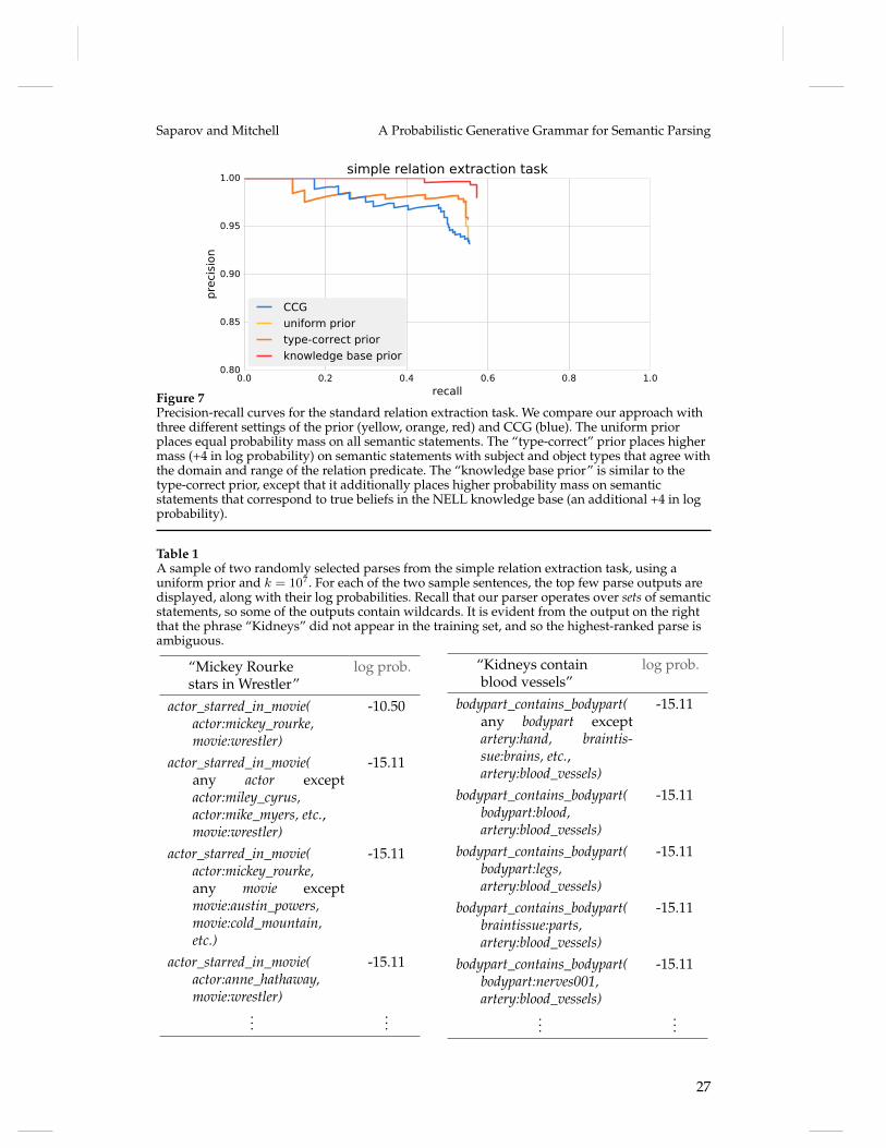
output semantic statement exactly matches the label. The main difficulty in this task isto learn the mapping between relations and the sentence text. For example, the datasetcontains verbs such as ‘makes’ which can refer to at least five NELL relations, includingcompanyeconomicsector, directordirectedmovie and musicartistgenre. The semantic types ofthe subject and object concepts are very informative in resolving ambiguity, and priorknowledge in the form of a belief system can further aid parsing. The precision-recallcurves in figure 7 were generated by sorting the outputs of our parser by posteriorprobability, which was computed using the top k = 10000 output parses for each testsentence (see section 6.4 for experiments with varying k).
We call a semantic statement “type-correct” if the subject and object concepts agreewith the domain and range of the instantiated relation, under the NELL ontology. Weexperimented with three prior settings for our parser: (1) uniform prior, (2) a priorwhere all type-correct semantic statements have a prior probability that is larger by 4units (in terms of log probability) than type-incorrect statements, and (3) a prior whereall semantic statements that correspond to true beliefs in the KB have a prior probabilitythat is 8 larger than type-incorrect statements and all type-correct correct statementshave probability 4 larger than type-incorrect statements.
In the simple relation extraction task, we find that CCG performs comparably toour parser under a uniform and type-correct prior. In fact, the parsers make the almostidentical predictions on the test sentences. The differences in the precision-recall curvesarise due to the differences in the scoring of predictions. The primary source of incorrectpredictions is when a noun in the test set refers to a concept in the ontology but doesnot refer to the same concept in the training set. For example, in the sentence “Wilsonplays guitar,” both parsers predict that “Wilson” refers to the politician Greg Wilson.The similarity in the performance of our parser with the uniform prior and the type-correct prior suggests that the parser learns “type-correctness” from the training data.This is due to the fact that, in our grammar, the distribution of the verb dependsjointly on the types of both arguments. With the KB prior, our parser outperforms CCG,demonstrating that our parser effectively incorporates background knowledge via thesemantic prior to improve precision and recall.
6.2 Modeling word morphology
In the second experiment, we demonstrate our parser’s ability to extract semanticinformation from the morphology of individual verbs, by operating over charactersinstead of preprocessed tokens. We generated a new labeled SVO dataset using aprocess similar to that in the first experiment. In this experiment, we did not restrict theverbs to the present tense. This dataset contains 3,197 sentences spanning 56 relationsand 2,166 concepts. The data was randomly split into a set of 2,538 training sentencesand 659 test sentences. We added a simple temporal model to the semantic formalism:all sentences in any past tense refer to semantic statements that were true in the past;all sentences in any present tense refer to presently true statements; and sentencesin any future tense refer to statements that will be true in the future. Thus the taskbecomes one of temporally-scoped relation extraction. A simple verb morphology modelwas incorporated into the grammar. Each verb is modeled as a concatenated root andaffix. In the grammar, the random selection of a production rule captures the selectionof the verb tense. The affix is selected deterministically according to the desired tenseand the grammatical person of the subject. The posterior probability of each parse wasestimated using the top k = 10000 parses for each test example. Results are shown infigure 8.
26
Saparov and Mitchell A Probabilistic Generative Grammar for Semantic Parsing
0.0 0.2 0.4 0.6 0.8 1.0
recall
0.80
0.85
0.90
0.95
1.00
pre
cisi
on
simple relation extraction task
CCG
uniform prior
type-correct prior
knowledge base prior
Figure 7Precision-recall curves for the standard relation extraction task. We compare our approach withthree different settings of the prior (yellow, orange, red) and CCG (blue). The uniform priorplaces equal probability mass on all semantic statements. The “type-correct” prior places highermass (+4 in log probability) on semantic statements with subject and object types that agree withthe domain and range of the relation predicate. The “knowledge base prior” is similar to thetype-correct prior, except that it additionally places higher probability mass on semanticstatements that correspond to true beliefs in the NELL knowledge base (an additional +4 in logprobability).
Table 1A sample of two randomly selected parses from the simple relation extraction task, using auniform prior and k = 107. For each of the two sample sentences, the top few parse outputs aredisplayed, along with their log probabilities. Recall that our parser operates over sets of semanticstatements, so some of the outputs contain wildcards. It is evident from the output on the rightthat the phrase “Kidneys” did not appear in the training set, and so the highest-ranked parse isambiguous.
“Mickey Rourkestars in Wrestler”
log prob.
actor_starred_in_movie(actor:mickey_rourke,movie:wrestler)
-10.50
actor_starred_in_movie(any actor exceptactor:miley_cyrus,actor:mike_myers, etc.,movie:wrestler)
-15.11
actor_starred_in_movie(actor:mickey_rourke,any movie exceptmovie:austin_powers,movie:cold_mountain,etc.)
-15.11
actor_starred_in_movie(actor:anne_hathaway,movie:wrestler)
-15.11
......
“Kidneys containblood vessels”
log prob.
bodypart_contains_bodypart(any bodypart exceptartery:hand, braintis-sue:brains, etc.,artery:blood_vessels)
-15.11
bodypart_contains_bodypart(bodypart:blood,artery:blood_vessels)
-15.11
bodypart_contains_bodypart(bodypart:legs,artery:blood_vessels)
-15.11
bodypart_contains_bodypart(braintissue:parts,artery:blood_vessels)
-15.11
bodypart_contains_bodypart(bodypart:nerves001,artery:blood_vessels)
-15.11
......
27

Computational Linguistics Volume xx, Number xx
0.0 0.2 0.4 0.6 0.8 1.0
recall
0.88
0.90
0.92
0.94
0.96
0.98
1.00pre
cisi
on
verb morphology relation extraction task
uniform prior
type-correct prior
knowledge base prior
CCG
uniform prior
type-correct prior
knowledge base prior
with simple grammar with verb morph. grammar
Figure 8Precision-recall curves for the temporally-scoped relation extraction task. We compare ourapproach with three different settings of the prior (yellow, orange, red) and CCG (blue). Thesolid lines denote our parser’s performance when using a grammar that models the morphologyof verbs, whereas the dashed lines are produced when our parser is trained with a grammar thatdoes not model verb morphology. The uniform prior places equal probability mass on allsemantic statements. The “type-correct” prior places higher mass (+4 in log probability) onsemantic statements with subject and object types that agree with the domain and range of therelation predicate. The “knowledge base prior” is similar to the type-correct prior, except that itadditionally places higher probability mass on semantic statements that correspond to truebeliefs in the NELL knowledge base (additional +4 in log probability).
In this temporally-scoped relation extraction task, our parser demonstrates bettergeneralization over verb forms. Our parser performs better when trained on a grammarthat models verb morphology (solid lines) than when trained on a simpler grammarthat does not consider the morphology of verbs (dashed lines). The parser is able to ac-complish this due to its ability to model the semantics in the morphology of individualwords. As in the first experiment, the performance of our parser improves when we usethe knowledge base prior, supporting the observation that our parser can effectivelyleverage background knowledge to improve its accuracy. There is, again, no differencein performance when using the uniform prior vs. the type-correct prior.
6.3 Out-of-vocabulary behavior
Recall that our parser operates over sets of semantic statements, as opposed to indi-vidual statements. Thus, it is possible that when parsing completes, the output is anon-singleton set of semantic statements that all share the highest probability parse.In our first two experiments, we counted these outputs as a “non-parse” to more fairlycompare with CCG. However, we can evaluate the quality of these ambiguous outputs.In figure 9, we again perform the simple relation extraction task with a modification: wemeasure the correctness of our parser’s output by whether the ground truth semanticstatement is contained within the set of semantic statements that share the highest prob-ability parse. CCG does not produce output on sentences that contain tokens which didnot appear in the training data. In a sense, this evaluation measures out-of-vocabularyperformance. Although precision is not as high as the in-vocabulary test, recall is much
28

Saparov and Mitchell A Probabilistic Generative Grammar for Semantic Parsing
0.0 0.2 0.4 0.6 0.8 1.0
recall
0.80
0.85
0.90
0.95
1.00
pre
cisi
on
simple relation extraction task (with ambiguous output)
CCG
uniform prior
type-correct prior
knowledge base prior
0.0 0.2 0.4 0.6 0.8 1.0
recall
0.0
0.2
0.4
0.6
0.8
1.0
pre
cisi
on
uniform prior
type-correct prior
knowledge base prior
Figure 9(top) Precision and recall for the simple relation extraction task, including unambiguousoutputs, and (bottom) on the subset of sentences for which CCG did not provide output. Wecompare our approach with three different settings of the prior (yellow, orange, red) and CCG(blue). The uniform prior places equal probability mass on all semantic statements. The“type-correct” prior places higher mass (+4 in log probability) on semantic statements withsubject and object types that agree with the domain and range of the relation predicate. The“knowledge base prior” is similar to the type-correct prior, except that it additionally placeshigher probability mass on semantic statements that correspond to true beliefs in the NELLknowledge base (additional +4 in log probability).
improved. The knowledge base prior again results in improved performance over theless informative priors.
6.4 Effect of changing the parameter k
In our parser, the search algorithm does not terminate until it has found the k-bestsemantic parses. This is useful for evaluating the confidence of the parser in its output,and for estimating the posterior probability of each parse. We examine the behavior ofthe parser as a function of k in figure 10. The timing results demonstrate that the parsercan scale to large knowledge bases while maintaining efficiency during parsing.
29

Computational Linguistics Volume xx, Number xx
100 101 102 103 104 105 106 107 108 109 10101011
k
0.0
0.2
0.4
0.6
0.8
1.0
are
a
AUC
AUC (with ambiguous output)
average parse time
0
500
1000
1500
2000
2500
mill
iseco
nds
behavior vs. k
Figure 10Area under the precision-recall curve and average parse time versus k, for the simple relationextraction task and a uniform prior. The dark green curve measures the area under theprecision-recall curve without considering ambiguous outputs (as in figure 7), whereas the lightgreen curve measures the area under the precision-recall curve taking into account theambiguous outputs (as in the top plot in figure 9)
Recall that, in order to produce the precision-recall curves for our parser’s output,we sort the outputs by their confidence scores (estimates of the posterior probability).In the figure, the area under the precision-recall curve (AUC) converges quickly at fairlysmall values of k, indicating that the relative ordering of the parse outputs convergesquickly. We found this behavior to be consistent for other choices of prior distributionsand for the more complex temporally-scoped relation extraction task. For values of ksmaller than∼ 106, the parser provides outputs very quickly. This is due to the fact that,as the parser performs its search, it can quickly find a set of semantic statements of sizeroughly 106 (e.g., when parsing “Federer plays golf”, it will quickly find an output thatlooks like athlete_plays_sport(athlete:roger_federer,*) where * is a wildcard that denotesany concept in the ontology). The parser will require additional time to search beyondthis initial ambiguous output. Note that this threshold value of k is identical to thenumber of concepts in the ontology: 1,786,741. The second threshold is likely relatedto the product of the number of concepts and the number of relations in the ontology:623 · 1786741 ≈ 1.11 · 109.
6.5 Out-of-knowledge base relation extraction
In all earlier experiments, we used a dataset that only contained sentences that refer tobeliefs in the NELL knowledge base. In order to inspect the performance of the parser onsentences that do not refer to NELL beliefs, we create a new dataset. We again start withthe SVO sentence corpus and modify the filtering process: we only accept sentences that(1) contain noun phrases that also exist in the first dataset (to ensure the parsers at leasthave a chance to unambiguously understand the sentences), (2) contain verb phrasesthat exist in the hand-constructed verb-relation map we used to create the first dataset,(3) cannot refer to any NELL belief, according to the can_refer_to instances andthe verb-relation map. More precisely, for every sentence, the can_refer_to relation
30
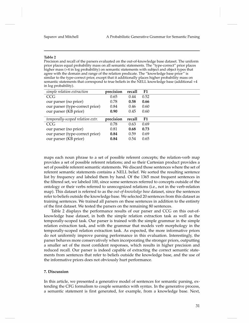
Saparov and Mitchell A Probabilistic Generative Grammar for Semantic Parsing
Table 2Precision and recall of the parsers evaluated on the out-of-knowledge base dataset. The uniformprior places equal probability mass on all semantic statements. The “type-correct” prior placeshigher mass (+4 in log probability) on semantic statements with subject and object types thatagree with the domain and range of the relation predicate. The “knowledge base prior” issimilar to the type-correct prior, except that it additionally places higher probability mass onsemantic statements that correspond to true beliefs in the NELL knowledge base (additional +4in log probability).
simple relation extraction precision recall F1CCG 0.65 0.44 0.52our parser (no prior) 0.78 0.58 0.66our parser (type-correct prior) 0.84 0.46 0.60our parser (KB prior) 0.90 0.45 0.60
temporally-scoped relation extr. precision recall F1CCG 0.78 0.63 0.69our parser (no prior) 0.81 0.68 0.73our parser (type-correct prior) 0.84 0.59 0.69our parser (KB prior) 0.84 0.54 0.65
maps each noun phrase to a set of possible referent concepts; the relation-verb mapprovides a set of possible referent relations; and so their Cartesian product provides aset of possible referent semantic statements. We discard those sentences where the set ofreferent semantic statements contains a NELL belief. We sorted the resulting sentencelist by frequency and labeled them by hand. Of the 1365 most frequent sentences inthe filtered set, we labeled 100, since some sentences referred to concepts outside of theontology or their verbs referred to unrecognized relations (i.e., not in the verb-relationmap). This dataset is referred to as the out-of-knowledge base dataset, since the sentencesrefer to beliefs outside the knowledge base. We selected 20 sentences from this dataset astraining sentences. We trained all parsers on these sentences in addition to the entiretyof the first dataset. We tested the parsers on the remaining 80 sentences.
Table 2 displays the performance results of our parser and CCG on this out-of-knowledge base dataset, in both the simple relation extraction task as well as thetemporally-scoped task. Our parser is trained with the simple grammar in the simplerelation extraction task, and with the grammar that models verb morphology in thetemporally-scoped relation extraction task. As expected, the more informative priorsdo not uniformly improve parsing performance in this evaluation. Interestingly, theparser behaves more conservatively when incorporating the stronger priors, outputtinga smaller set of the most confident responses, which results in higher precision andreduced recall. Our parser is indeed capable of extracting the correct semantic state-ments from sentences that refer to beliefs outside the knowledge base, and the use ofthe informative priors does not obviously hurt performance.
7. Discussion
In this article, we presented a generative model of sentences for semantic parsing, ex-tending the CFG formalism to couple semantics with syntax. In the generative process,a semantic statement is first generated, for example, from a knowledge base. Next,
31

Computational Linguistics Volume xx, Number xx
the tree is constructed top-down using a recursive procedure: production rules areselected randomly, possibly depending on features of the semantic statement. Semantictransformation operations specify how to decompose the semantic statement in orderto continue recursion. We presented a particular construction where production rulesare selected using an HDP. We applied MCMC to perform inference in this model, andconstructed a chart-driven agenda parser. Our application of the HDP is distinct fromprevious uses, since in our construction, the path indicator for each observation is notassumed to be fixed. We evaluate our parser on a dataset of SVO sentences, labeledwith semantic statements from NELL. The results demonstrate that our parser canincorporate prior knowledge from a knowledge base via the semantic prior. With aninformative prior, our parser outperforms a state-of-the-art CCG parser. In addition, wedemonstrate that our model can be used to jointly model the morphology of individualverbs, leading to improved generalization over verbs in a temporally-scoped relationextraction task. The results indicate that our framework can scale to knowledge bases,such as NELL, with millions of beliefs, and can be extended to more complex grammarsand richer semantic formalisms without sacrificing exact inference and the principlednature of the model.
An interesting parallel can be drawn between our inference problem and the prob-lem of finding shortest paths in hypergraphs. Similar parallels have been drawn inother parsers (Klein and Manning 2001, 2003a; Pauls and Klein 2009; Pauls, Klein, andQuirk 2010). Since our approach is top-down, the specification of our hypergraph ismore involved. Imagine a hypergraph containing a vertex for every semantic statementx ∈ X , a vertex for every intermediate rule state A→ B1 . . .Bk • Bk+1 . . .Bn, and twovertices for every nonterminal (one indicating that parsing is incomplete and one forcompleted parses). Add a hyperedge to this graph for every allowable operation by theparser. A hyperedge is a generalization of an edge where both its “head” and “tail” canbe sets of vertices. Then, the problem of parsing can be equivalently stated as finding theshortest “path” from two sets of vertices: the source set of vertices are those representingthe incomplete S nonterminal and all elements of XS , and the destination vertex is thecomplete S nonterminal. See Gallo, Longo, and Pallottino (1993), Klein and Manning(2001) for definitions and further details. Our algorithm can then be understood as anapplication of A∗ search for the k-best paths in this hypergraph. The monotonicity prop-erty of our algorithm is a consequence of Dijkstra’s theorem generalized to hypergraphs(Gallo, Longo, and Pallottino 1993). This also suggests that our parser can be improvedby utilizing a tighter heuristic.
In the parser, the prior contribution is rather loosely incorporated into the objective(equation 38). This is due to the fact that we assumed nothing about the structure of thesemantic prior. However, the algorithm could potentially be made more efficient if wecould factorize the prior, for example, over nonterminals or rules in the grammar. Thiscould provide an additive term to equation 38.
We presented our inference approach as a combination of two search algorithms: (1)the HDP inference component, and (2) the joint syntactic-semantic parser. However, itis possible to merge these two searches into a single search (the priority queues of eachalgorithm would be unified into a single global priority queue), potentially improvingthe overall efficiency.
In this article, we showed how to utilize HDPs to add dependence between seman-tic features and the probabilistic selection of production rules in the generative process.It would be interesting to explore the application of other dependent Dirichlet processesand random probability measures, possibly as a means to induct a grammar in ourframework.
32

Saparov and Mitchell A Probabilistic Generative Grammar for Semantic Parsing
Another highly promising avenue of research is to explore more complex priorstructures. For instance, a generative model of a knowledge base could be composedwith the framework we present here. This would result in a parser that would learnnew beliefs as it reads text. Another direction is to model the generation of a sequenceof sentences (such as in a paragraph), where complex relationships between conceptsbridge across multiple sentences. Such an approach would likely contain a model ofcontext shared across sentences. An example of such a generative process would be to“generate” a representation of the document context using a background knowledgebase. Then, semantic statements for each sentence in the document can be generatedfrom this intermediate document-level representation in addition to other sources ofdocument-level information. Finally, our grammar would generate sentences for eachsemantic statement. The problem of co-reference resolution also becomes more apparentin these settings with more complex sentences. In both the single-sentence and multiple-sentence settings, co-reference resolution can be integrated into parsing. Incorporatingthese extensions into a richer unified parsing framework would be promising.
Acknowledgments
We thank Emmanouil A. Platanios and Jayant Krishnamurthy for the insightful discus-sion and helpful comments on the draft. We also thank anonymous reviewers for theirfeedback on the shortened version of this manuscript. This work was supported in partby NSF grant IIS1250956, and in part by DARPA DEFT contract FA87501320005.
ReferencesAdams, Beverly Colwell, Laura C. Bell, and Charles A. Perfetti. 1995. A trading relationship
between reading skill and domain knowledge in children’s text comprehension. DiscourseProcesses, 20(3):307–323. 2
Aho, Albert V. and Jeffery D. Ullman. 1972. The Theory of Parsing, Translation, and Compiling,volume 1. Prentice-Hall, Englewood Cliffs, NJ. 4
Aldous, David J. 1985. Exchangeability and related topics. In École d’été de probabilités deSaint-Flour, XIII—1983, volume 1117 of Lecture Notes in Math. Springer, Berlin, pages 1–198. 5
Anderson, Richard C. and P. David Pearson. 1984. A schema-theoretic view of basic processes inreading comprehension. University of Illinois at Urbana-Champaign Champaign, Ill. : Bolt,Beranek, and Newman Inc. 2
Baker, Collin F., Charles J. Fillmore, and John B. Lowe. 1998. The berkeley FrameNet project. InProceedings of the 17th International Conference on Computational Linguistics, volume 1, pages86–90, Montreal, Quebec, Canada. Association for Computational Linguistics. 3
Banarescu, Laura, Claire Bonial, Shu Cai, Madalina Georgescu, Kira Griffitt, Ulf Hermjakob,Kevin Knight, Philipp Koehn, Martha Palmer, and Nathan Schneider. 2013. Abstract meaningrepresentation for sembanking. 3
Berger, Adam, Stephen Della Pietra, and Vincent Della Pietra. 1996. A maximum entropyapproach to natural language processing. Computational Linguistics, 22:39–71. 12
Bloom, Paul. 2000. How Children Learn the Meanings of Words. MIT Press, Cambridge, MA. 2Bordes, Antoine, Xavier Glorot, Jason Weston, and Yoshua Bengio. 2012. Joint learning of words
and meaning representations for open-text semantic parsing. In Neil D. Lawrence and MarkGirolami, editors, AISTATS, volume 22 of JMLR Proceedings, pages 127–135. JMLR.org. 1
Callan, Jamie, Mark Hoy, Changkuk Yoo, and Le Zhao. 2009. The clueweb09 dataset. 25Chomsky, N., editor. 1957. Syntactic structures. Mouton & Co., The Hague. 4Chomsky, Noam. 1956. Three models for the description of language. IRE Transactions on
Information Theory, 2:113–124. 4, 11Church, A. 1932. A set of postulates for the foundation of logic part i. Annals of Mathematics,
33(2):346–366. 3Cohen, Shay B., David M. Blei, and Noah A. Smith. 2010. Variational inference for adaptor
grammars. In HLT-NAACL, pages 564–572. The Association for Computational Linguistics. 4
33

Computational Linguistics Volume xx, Number xx
Durrett, Greg and Dan Klein. 2014. A joint model for entity analysis: Coreference, typing, andlinking. TACL, 2:477–490. 5
Earley, Jay. 1970. An efficient context-free parsing algorithm. Communications of the ACM,6(8):451–455. Reprinted in Grosz et al. (1986). 19
Ferguson, Thomas S. 1973. A Bayesian analysis of some nonparametric problems. The Annals ofStatistics, 1(2):209–230. 5
Fincher-Kiefer, Rebecca. 1992. The role of prior knowledge in inferential processing. Journal ofResearch in Reading, 15:12–27. 2
Finkel, Jenny Rose and Christopher D. Manning. 2009. Joint parsing and named entityrecognition. In HLT-NAACL, pages 326–334. The Association for Computational Linguistics. 1
Finkel, Jenny Rose and Christopher D. Manning. 2010. Hierarchical joint learning: Improvingjoint parsing and named entity recognition with non-jointly labeled data. In Jan Hajic, SandraCarberry, and Stephen Clark, editors, ACL, pages 720–728. The Association for ComputerLinguistics. 1
Gallo, Giorgio, Giustino Longo, and Stefano Pallottino. 1993. Directed hypergraphs andapplications. Discrete Applied Mathematics, 42(2):177–201. 4, 32
Gelfand, Alan E. and Adrian F. M. Smith. 1990. Sampling-based approaches to calculatingmarginal densities. Journal of the American Statistical Association, 85(410):398–409. 6
Hockenmaier, Julia. 2001. Statistical parsing for ccg with simple generative models. In ACL(Companion Volume), pages 7–12. CNRS, Toulose, France. 12
Hockenmaier, Julia and Mark Steedman. 2002. Generative models for statistical parsing withcombinatory categorial grammar. In ACL, pages 335–342. ACL. 12
Jäger, Gerhard. 2004. Anaphora and type logical grammar. UniversitÃd’tsbibliothek JohannChristian Senckenberg. 12
Johnson, Mark and Katherine Demuth. 2010. Unsupervised phonemic chinese wordsegmentation using adaptor grammars. In Chu-Ren Huang and Dan Jurafsky, editors,COLING, pages 528–536. Tsinghua University Press. 4
Johnson, Mark, Thomas L. Griffiths, and Sharon Goldwater. 2007. Adaptor grammars: Aframework for specifying compositional nonparametric Bayesian models. In Advances inNeural Information Processing Systems (NIPS). 4
Kazama, Jun’ichi and Kentaro Torisawa. 2007. Exploiting wikipedia as external knowledge fornamed entity recognition. In Joint Conference on Empirical Methods in Natural LanguageProcessing and Computational Natural Language Learning, pages 698–707. 1
Kim, J. and D. Moldovan. 1995. Acquisition of linguistic patterns for knowledge-basedinformation extraction. IEEE Transactiops on Knowledge and Data Engineering, 7(5):713–724. 5
Klein, Dan and Christopher D. Manning. 2001. Parsing and hypergraphs. In IWPT. TsinghuaUniversity Press. 4, 32
Klein, Dan and Christopher D. Manning. 2003a. A* parsing: Fast exact viterbi parse selection. InHLT-NAACL. 4, 32
Klein, Dan and Christopher D. Manning. 2003b. Fast exact inference with a factored model fornatural language parsing. In In Advances in Neural Information Processing Systems 15 (NIPS). 22
Krishnamurthy, Jayant and Tom M. Mitchell. 2014. Joint syntactic and semantic parsing withcombinatory categorial grammar. In Proceedings of the 52nd Annual Meeting of the Association forComputational Linguistics (Volume 1: Long Papers), pages 1188–1198, Baltimore, Maryland, June.Association for Computational Linguistics. 5, 25
Li, Junhui, Muhua Zhu, Wei Lu, and Guodong Zhou. 2015. Improving semantic parsing withenriched synchronous context-free grammar. In Lluís Màrquez, Chris Callison-Burch, Jian Su,Daniele Pighin, and Yuval Marton, editors, EMNLP, pages 1455–1465. The Association forComputational Linguistics. 4
Liang, Percy, Michael I. Jordan, and Dan Klein. 2013. Learning dependency-based compositionalsemantics. Computational Linguistics, 39(2):389–446. 3
Merlo, Paola and Gabriele Musillo. 2008. Semantic parsing for high-precision semantic rolelabelling. In Alexander Clark and Kristina Toutanova, editors, CoNLL, pages 1–8. ACL. 1
Mitchell, T., W. Cohen, E. Hruscha, P. Talukdar, J. Betteridge, A. Carlson, B. Dalvi, M. Gardner,B. Kisiel, J. Krishnamurthy, N. Lao, K. Mazaitis, T. Mohammad, N. Nakashole, E. Platanios,A. Ritter, M. Samadi, B. Settles, R. Wang, D. Wijaya, A. Gupta, X. Chen, A. Saparov,M. Greaves, and J. Welling. 2015. Never-ending learning. In AAAI. : Never-Ending Learning inAAAI-2015. 25
34

Saparov and Mitchell A Probabilistic Generative Grammar for Semantic Parsing
Nakashole, Ndapandula and Tom M. Mitchell. 2015. A knowledge-intensive model forprepositional phrase attachment. In ACL (1), pages 365–375. The Association for ComputerLinguistics. 5
Ng, Vincent. 2007. Shallow semantics for coreference resolution. In IJCAI, pages 1689–1694. 1Pauls, Adam and Dan Klein. 2009. K-best a* parsing. In Keh-Yih Su, Jian Su, and Janyce Wiebe,
editors, ACL/IJCNLP, pages 958–966. The Association for Computer Linguistics. 4, 32Pauls, Adam, Dan Klein, and Chris Quirk. 2010. Top-down k-best a* parsing. In Proceedings of the
ACL 2010 Conference Short Papers, ACLShort ’10, pages 200–204, Stroudsburg, PA, USA.Association for Computational Linguistics. 4, 32
Ponzetto, S. P. and M. Strube. 2006. Exploiting semantic role labeling, WordNet and Wikipediafor coreference resolution. Proceedings of the main conference on Human Language TechnologyConference of the North American Chapter of the Association of Computational Linguistics, pages192–199. 1
Prokofyev, Roman, Alberto Tonon, Michael Luggen, Loic Vouilloz, Djellel Eddine Difallah, andPhilippe CudrÃl’-Mauroux. 2015. Sanaphor: Ontology-based coreference resolution. InMarcelo Arenas, ÃSscar Corcho, Elena Simperl, Markus Strohmaier, Mathieu d’Aquin,Kavitha Srinivas, Paul T. Groth, Michel Dumontier, Jeff Heflin, Krishnaprasad Thirunarayan,and Steffen Staab, editors, International Semantic Web Conference (1), volume 9366 of LectureNotes in Computer Science, pages 458–473. Springer. 5
Ratinov, Lev-Arie and Dan Roth. 2012. Learning-based multi-sieve co-reference resolution withknowledge. In Jun’ichi Tsujii, James Henderson, and Marius Pasca, editors, EMNLP-CoNLL,pages 1234–1244. ACL. 5
Ratnaparkhi, Adwait. 1998. Maximum entropy models for natural language ambiguityresolution. PhD thesis. 12
Robert, C. P. and G. Casella. 2010. Monte Carlo Statistical Methods. Springer, New York, NY. 6Salloum, Wael. 2009. A question answering system based on conceptual graph formalism.
volume 3. IEEE CS Press. 5Salton, Gerald. 1971. The SMART Retrieval System: Experiments in Automatic Document Processing.
Prentice Hall. 3Steedman, Mark. 1996. Surface structure and interpretation. Linguistic inquiry monographs, 30.
MIT Press. 12Talukdar, Partha Pratim, Derry Tanti Wijaya, and Tom M. Mitchell. 2012. Acquiring temporal
constraints between relations. In Xue wen Chen, Guy Lebanon, Haixun Wang, andMohammed J. Zaki, editors, CIKM, pages 992–1001. ACM. 25
Tanaka, Takaaki, Francis Bond, Timothy Baldwin, Sanae Fujita, and Chikara Hashimoto. 2007.Word sense disambiguation incorporating lexical and structural semantic information. InEMNLP-CoNLL, pages 477–485. ACL. 1
Teh, Yee Whye, Michael I. Jordan, Matthew J. Beal, and David M. Blei. 2006. Hierarchicaldirichlet processes. Journal of the American Statistical Association, 101(476):1566–1581. 4, 6, 7, 10
Turney, Peter D. and Patrick Pantel. 2010. From frequency to meaning: Vector space models ofsemantics. CoRR, abs/1003.1141. 3
Wong, Yuk Wah and Raymond J. Mooney. 2006. Learning for semantic parsing with statisticalmachine translation. In Robert C. Moore, Jeff A. Bilmes, Jennifer Chu-Carroll, and MarkSanderson, editors, HLT-NAACL. The Association for Computational Linguistics. 4
Wong, Yuk Wah and Raymond J. Mooney. 2007. Learning synchronous grammars for semanticparsing with lambda calculus. In John A. Carroll, Antal van den Bosch, and Annie Zaenen,editors, ACL. The Association for Computational Linguistics. 4
35

36
![BayesOWL: Uncertainty Modeling in Semantic Web … Uncertainty Modeling in Semantic Web Ontologies 5 inference with general DAG structure is NP-hard [3], BN inference algorithms such](https://img.dokumen.tips/doc/110x75/5ad9838a7f8b9a53618b5bea/bayesowl-uncertainty-modeling-in-semantic-web-uncertainty-modeling-in-semantic.jpg)


![Semantic Segmentation with Second-Order PoolingSemantic Segmentation with Second-Order Pooling 3 generative [12] or discriminative [13] frameworks. These techniques are very pow-erful,](https://img.dokumen.tips/doc/110x75/5a7bff5b7f8b9a66798c760e/semantic-segmentation-with-second-order-poolingsemantic-segmentation-with-second-order.jpg)


![Semantic roles - Universitetet i oslo · Semantic roles Semantic (thematic) roles Introduced in generative grammar mid-1960s and early 70s [Fillmore 1968, Jackendoff 1972] Classify](https://img.dokumen.tips/doc/110x75/5eac755f2f224c3e2d4387cb/semantic-roles-universitetet-i-oslo-semantic-roles-semantic-thematic-roles-introduced.jpg)


![Adjectives - Semantic Characteristicsocw.nctu.edu.tw/course/syntax/W3III.pdf · Adjectives: Syntactic behavior Adjectival Predicate: – Joe [is smart] Modifier in NP: – Joe is](https://img.dokumen.tips/doc/110x75/5fcfc122b8946860f776fc97/adjectives-semantic-adjectives-syntactic-behavior-adjectival-predicate-a-joe.jpg)