Embed Size (px)
Citation preview

A Positive Theory of Economic Growth and theDistribution of Income∗
Allan H. MeltzerThe Tepper School
Carnegie-Mellon UniversityPittsburgh, PA
Scott F. RichardThe Wharton School
University of PennsylvaniaPhiladelphia, PA
First Draft: July 4, 2014Current Draft: October 10, 2014
c©Allan H. Meltzer and Scott F. RichardAll Rights Reserved
Abstract
This paper is a positive theory of the distribution of income and thegrowth rate of the economy. It builds on our earlier work, Meltzer and Richard (1981),on the size of government. How does the distribution of income change asan economy grows? To answer this question we build a model of a laboreconomy in which consumers have diverse productivity. The governmentimposes a linear income tax which funds equal per capita redistribution.The tax rate is set in a sequence of single issue election in which the me-dian productivity individual is decisive. Economic growth is the resultof using a learning by doing technology, so higher taxes discourage laborcausing the growth rate of the economy to fall. The distribution of pro-ductivity can widen due to increased technological specialization. Thiscauses voters to raise the equilibrium tax rate and reduce growth. Thedistribution of pre-tax income widens. We estimate the model using datafrom the U.S., U.K. and France with excellent results.
1 Introduction
How does the distribution of income change as economic growth changes? Howdoes growth change when governments raise tax rates to finance increased re-distribution? Economists have discussed these issues for decades, and they haverecently become major political issues in developed economies.
∗We wish to thank V.V. Chari, Marvin Goodfriend and the seminar particpants at theWharton School fo useful comments.
1
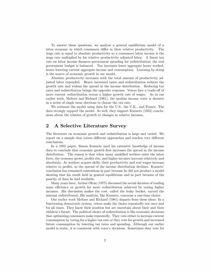
To answer these questions, we analyze a general equilibrium model of alabor economy in which consumers differ in their relative productivity. Thewage rate is equal to absolute productivity so a consumers labor income is thewage rate multiplied by his relative productivity adjusted labor. A linear taxrate on labor income finances government spending for redistribution; the realgovernment budget is balanced. Tax increases lower aggregate hours worked,hence lowering current aggregate income and consumption. Learning-by-doingis the source of economic growth in our model.Absolute productivity increases with the total amount of productivity ad-
justed labor expended. Hence increased taxes and redistribution reduces thegrowth rate and widens the spread in the income distribution. Reducing taxrates and redistribution brings the opposite response. Voters face a trade-off ofmore current redistribution versus a higher growth rate of wages. As in ourearlier work, Meltzer and Richard (1981), the median income voter is decisivein a series of single issue elections to choose the tax rate.We estimate the model using data for the U.S., the U.K., and France. The
data strongly support the model. As well, they support Kuznets (1955) conclu-sions about the relation of growth to changes in relative incomes.
2 A Selective Literature Survey
The literature on economic growth and redistribution is large and varied. Wereport on a sample that covers different approaches and reaches very differentconclusions.In a 1955 paper, Simon Kuznets used his extensive knowledge of income
data to conclude that economic growth first increases the spread in the incomedistribution. The reason is that when many unskilled workers enter the laborforce, the economy grows, profits rise, and higher incomes increase relatively andabsolutely. As workers acquire skills, their productivity and real wages increaserelative to profits, so the spread of the income distribution declines. Kuznets’conclusion has remained contentious in part because he did not produce a modelshowing that his result held in general equilibrium and in part because of thepaucity of data he had available.Many years later, Arthur Okun (1975) discussed the social decision of trading
some effi ciency or growth for more redistribution achieved by taxing higherincomes. His discussion makes the cost, called the leaky bucket, exceed theamount redistributed. His analysis, like Kuznets, concerns a one-time choice.Our earlier work Meltzer and Richard (1981) departs from these ideas. In a
functioning democratic system, voters make the choice repeatedly not once andfor all times. They know their position but are uncertain about their and theirchildren’s future. The political choice of redistribution is like economic decisionsthat optimizing consumers make repeatedly. They vote either to increase currentconsumption by voting for a higher tax rate or they vote for growth and increasedfuture consumption by lowering tax rates and spending. Although our earliermodel is static, it is consistent with voter’s decisions. Sometimes they vote for
2
higher tax rates and spending and sometimes they do the opposite. No societychooses once for all future time.Much of the recent literature on economic growth focusses on the role of
capital as summarized in the influential book by Acemoglu (2009). We thinkthat the emphasis in explaining growth should be on labor productivity notcapital. Over the past 200 years real wages have increased 20 fold while thereturn to capital has remained basically unchanged. Politically, if capital de-termines growth it is diffi cult to understand why the taxes on capital incomehave risen, especially since capital is owned almost exclusively by the upper halfof the income distribution. So we choose to ignore capital and focus on laborproductivity as the exclusive engine of growth.1
Treatment of high incomes as rent permits increased taxation to financeredistribution without reducing productive activity. A special use of rents isthe claim that most high incomes result from inheritance of wealth producedby an earlier generation and passed on. Evidence does not support this claimboth in the U.S. and other developed countries. Kaplan and Rauh, (2013,46, 48); Becker and Tomes (1979, 1158). Some work suggests that cultureand educational attainment of parents has more important influence on latergenerations than financial inheritance. Becker and Tomes (1979, 1191), Corak(2013, 80)Another problem with treating high incomes, for example those of the top
one percent, as rent is that the population is not fixed but changes. Piketty(2014, 115-16) writes that capital transforms “itself into rents as it accumu-lates in large enough amounts.” Saez (2013, 24) concludes that “high top taxrates reduce the pre-tax income gap without visible effect on economic growth.”Corak (2013) shows that intergenerational mobility remains large in developedcountries like the U.S. and Canada. The main exception in the U.S. is the“least advantaged.” In this paper we address the issue of why some of the leastadvantaged have stagnant incomes. The least productive choose not to work,so their incomes are all redistribution. Hence they do not acquire productiveskills.Much of the discussion of the top one percent makes no mention of the other
99 percent. Often, the focus is on income from capital, which neglects laborincome, about 70% of total income. A very different explanation of the risingshare of income earned by the top one percent builds on work on superstarsby Rosen (1981). Rosen argued that technological change increases the relativeproductivity of individuals with exceptional talent in using and developing thenew technology. Rosen’s work brings in relative productivity as an explanationof the rising share of the top one percent. Developing new software, like SteveJobs and others, that create entire markets brings high rewards. Successfullymanaging a bank or corporation with branches in 50 or 100 countries is an orderof magnitude more diffi cult than managing in a single country or state. Tenyears is a long tenure in such jobs, so there is turnover not inheritance of high
1Piguillem and Schneider (2013) add majority rule voting to the neoclassical growth model.They show that the median voter is decisive assuming that the distribution of capital is strictlyproportional to the distribution of relative productivity.
3
income positions. Highly skilled surgeons adept at operating new technologiesshould be included.Major league sport stars in football, baseball, soccer, basketball and hockey
no longer perform before audiences restricted to a stadium. Television increasedtheir productivity. Kaplan and Rauh (2013, 42, Figure 3) show the substantialincrease in their incomes. Turnover is high; careers at the top are brief. Andthere is little evidence that the super stars cede their places to their offspring.Rock musicians and entertainment stars often have similar careers with highincomes for short duration. Income of super stars may explain some of theincrease in the relative earnings of the top one percent. We doubt that it isa full explanation because the data after 1980 show that the rise in the pre-tax share of the top one percent can be seen in data for the United States, theUnited Kingdoms, Canada and Sweden but data for France and the Netherlandsdo not show a similar increase. Roine and Waldenstrom (2006)The share of pre-tax incomes received by the top one percent includes income
from reported capital gains. That makes it more volatile, rising in periods whenowners of shares choose to report gains in excess of losses. Also there aresubstantial differences in the relative shares of different income quintiles whenbefore and after tax and transfers are included. Most economic theory considersconsumption, based on permanent not current income, to be a better measure ofthe economic component of well-being. Table 1 shows data on pre- and post-taxincomes for the United States. The data for 1979 to 2010 are available on theCongressional Budget Offi ce website.2
2http://www.cbo.gov/publication/44604
4
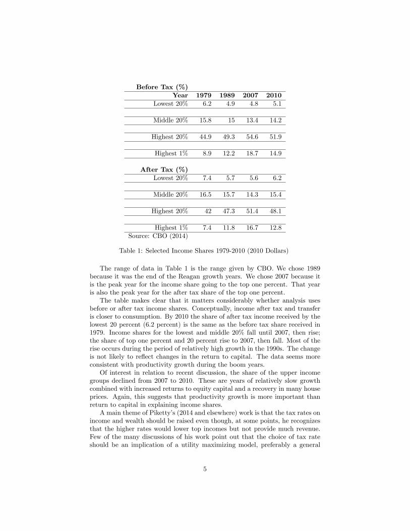
Before Tax (%)Year 1979 1989 2007 2010
Lowest 20% 6.2 4.9 4.8 5.1
Middle 20% 15.8 15 13.4 14.2
Highest 20% 44.9 49.3 54.6 51.9
Highest 1% 8.9 12.2 18.7 14.9
After Tax (%)Lowest 20% 7.4 5.7 5.6 6.2
Middle 20% 16.5 15.7 14.3 15.4
Highest 20% 42 47.3 51.4 48.1
Highest 1% 7.4 11.8 16.7 12.8Source: CBO (2014)
Table 1: Selected Income Shares 1979-2010 (2010 Dollars)
The range of data in Table 1 is the range given by CBO. We chose 1989because it was the end of the Reagan growth years. We chose 2007 because itis the peak year for the income share going to the top one percent. That yearis also the peak year for the after tax share of the top one percent.The table makes clear that it matters considerably whether analysis uses
before or after tax income shares. Conceptually, income after tax and transferis closer to consumption. By 2010 the share of after tax income received by thelowest 20 percent (6.2 percent) is the same as the before tax share received in1979. Income shares for the lowest and middle 20% fall until 2007, then rise;the share of top one percent and 20 percent rise to 2007, then fall. Most of therise occurs during the period of relatively high growth in the 1990s. The changeis not likely to reflect changes in the return to capital. The data seems moreconsistent with productivity growth during the boom years.Of interest in relation to recent discussion, the share of the upper income
groups declined from 2007 to 2010. These are years of relatively slow growthcombined with increased returns to equity capital and a recovery in many houseprices. Again, this suggests that productivity growth is more important thanreturn to capital in explaining income shares.A main theme of Piketty’s (2014 and elsewhere) work is that the tax rates on
income and wealth should be raised even though, at some points, he recognizesthat the higher rates would lower top incomes but not provide much revenue.Few of the many discussions of his work point out that the choice of tax rateshould be an implication of a utility maximizing model, preferably a general
5

equilibrium model, such as in this paper.Long before the Piketty book stimulated renewed interest in income distri-
bution and the choice of tax rate, Becker and Tomes (1979, 1986) developedgeneral equilibrium models of income distribution across family generations.Becker and Tomes (1979)1175 choose a linear tax structure and use revenuesfor redistribution. They find that “even a progressive tax and public expendi-ture system may widen the inequality of disposable income.”Becker and Tomes(1986, 533-4) note that some empirical work by Arthur Goldberger found thatthe widening of inequality does not occur for several generations.Alesina and Rodick (1994) use a growth model. As in Meltzer and Richard (1981)
voters differ in their endowments, some prefer more, some less, taxation and gov-ernment spending. The authors show that, in general, voters will not maximizeeconomic growth. Instead, they vote to tax capital to finance redistribution. Asin all general equilibrium models, the budget is balanced.Alesina and Rodrik use the Gini coeffi cient to measure income inequality.
They show empirically that income inequality is negatively related to futureeconomic growth. The reason is that as income inequality rises, voters choosemore redistribution, reducing the growth rate.May increased government spending and taxation increase both growth and
redistribution? Of course, it may, but the empirical data in Alesina and Rodrikand elsewhere shows that, in developed economies, the reverse is true. Govern-ment spending is mainly for redistribution to augment consumption.Our contribution to this research builds on the findings in Alesina and Ro-
drik but incorporates some of the principal ideas offered by Simon Kuznetsin his insightful discussions. Kuznets (1979) contains several of his essays. Inparticular we incorporate technological change Kuznets (1979, 45) as a majorsource of income growth with substantial effects on income distribution that arenot explicitly considered in much of the literature.In our model, growth of labor productivity and labor income — learning
by doing — is a large factor, the largest, in explaining growth of output andliving standards. We do not challenge the role of capital or the implicationthat the return to capital changes very little. The return to labor changesmuch more. We do not impose our ideas of the desirable extent of incomedistribution. The workers in our model are voters who choose their preferredtax rate and redistribution. They are aware that an increased tax rate to financeredistribution lowers investment in productivity enhancing investments that addto their future consumption.Our analysis fits the contours of growth experience. As workers learn, their
skills, productivity and incomes increase. They save more, acquire real assetsespecially housing. They spend to educate their offspring, and they vote for oragainst redistribution and taxation. In our earlier work,Meltzer and Richard (1981),we showed that rational voters choose a tax rate consistent with the most basiceconomic theory. They decide whether they want increased taxes to financemore redistribution (consumption today), or lower tax rates to spur investmentand future consumption. In the growth model here, the same choice remainscentral.
6

3 The Economic Model
We begin by modeling consumers and calculating their lifetime consumption bymaximizing their utility. Consumers are endowed with different relative levelsof productivity, indexed by n, and one unit of time. A consumer with relativeproductivity n maximizes his lifetime utility of consumption and leisure:
V n(cn, `n) =
∫ ∞0
e−δt [λ ln(cnt ) + (1− λ) ln(1− `nt )] dt, (1)
where cn = {cnt }∞0 is his consumption stream, `n = {`nt }∞0 is his labor stream,and δ is the discount rate. There is a government which levies a linear tax onincome at rate τ t at time t and uses the proceeds for redistribution, equally percapita. The budget constraint for a consumer with productivity n is
cnt = ρtwt + (1− τ t)wtn`nt , (2)
where nwt is the wage per unit of labor at time t and ρtwt is amount redistrib-uted at time t. Each individual is a price taker in the labor market, takes theprocesses {ρt}, {wt}, and {τ t} as given and chooses {cnt } and {`nt } to maximizeutility. The standard Bellman equation for optimal control is3
0 = max[λ ln(cnt ) + (1− λ) ln(1− `nt )− δJn + Jnw
�wt + Jnρ
�ρt + Jnτ
�τ t
], (3)
where Jn(wt, ρt, τ t) is the value function for a consumer with relative produc-tivity n. The standard first-order conditions for equation (3) yield
`nt = λ− ρt(1− λ)
n(1− τ t). (4)
The maximum fraction of time devoted to working is λ, as can be seen by settingρt = 0 in equation (4). Since labor must be positive there is a minimum levelof relative productivity, νt, below which consumers are voluntarily unemployed,living on their redistribution:
νt =ρt(1− λ)
λ(1− τ t). (5)
We call νt the voluntary unemployment productivity. Optimal consumption is
cnt = ρtwt, for n < νt. (6a)
= λ(ρt + (1− τ t)n)wt, for n ≥ νt. (6b)
Notice that consumption is increasing and ordered by relative productivity forall choices of ρt and τ t.
3The super dot indicates the time derivative.Adding stochastic terms to the state equations changes the value function Jn, but does not
change the consumers optimal decisions state contingent decisions.
7

Relative productivity is distributed lognormally, lnn ∼ N(0, σt), so thatthe median relative productivity is m = 1 and the mean relative productivityis nt = e
12σt > 1. Hence nwt is the absolute productivity of a consumer with
relative productivity n. Since the median consumer has productivity m = 1,wt is the absolute productivity of the median consumer.To understand how productivity and economic growth affect the income
distribution and redistribution in a mature economy such as the U.S. or westernEurope, we need to consider change in relative productivity, σt, as well as changein absolute productivity, wt. An increase in wt increases the wage earned by allworkers, regardless of their level of productivity. An increase in σt is meantto capture the effect of technological change with disparate effects, such as thecomputerization of production the U.S. experienced in the past 40 years. Meanproductivity normalized hours worked at time t, Ψt, is:
Ψt =
∞∫νt
n`nt exp(− 12 ( lnnσt )2)
nσt√
2πdn
=
∞∫νt
λ(n− νt) exp(− 12 ( lnnσt )2)
nσt√
2πdn
= λ
[ntN(− ln νt
σt+ σt)− νtN(− ln νt
σt)
]. (7)
The government’s budget is balanced in that the per capita spending onredistribution, wtρt, equals the tax revenues, wtΨtτ t:
wtτ tΨt = wtρt. (8)
Everything in this economy is a function of νt, σt and wt. It is obviousfrom equation (7) that Ψt is a function of σt and νt. Substituting equation (5)into equation (4) we find that
`nt = λ(1− νtn
). (9)
Solving equation (8) for ρt, substituting the result into equation (5) and thensolving for τ t gives:
τ t =νt
νt + (1− λ)ψt(10)
where
ψt = Ψt/λ = ntN(− ln νtσt
+ σt)− νtN(− ln νtσt
) (11)
is the average fraction of full-time equivalent, productivity-adjusted, units worked.Substituting equation (10) into equation (8) gives:
ρt =λνtψt
νt + (1− λ)ψt. (12)
8
Finally, substituting equations (9), (10), and (12) into equation (6) gives:
cnt = λwtψtνt
νt + (1− λ)ψt, for n < νt. (13a)
= λwtψtλνt + (1− λ)n
νt + (1− λ)ψt, for n ≥ νt. (13b)
In preparation for determining the size of government we show that selectingνt is an equivalent to selecting τ t. This can be seen by showing that τ t is astrictly increasing function of νt :
dτ tdνt
=(1− λ)ntN(− ln νtσt
+ σt)
(νt + (1− λ)ψt)2
> 0. (14)
Hence the mapping from νt to τ t is continuous and strictly increasing, so thatsetting νt is equivalent to setting τ t. Furthermore, increasing (decreasing) νt isequivalent to increasing (decreasing) τ t.
Finally, we determine the mean number of labor units worked per capita,`t :
`t =
∞∫νt
`nt exp(− 12 ( lnnσt )2)
nσt√
2πdn (15)
=
∞∫νt
λ(1− νt/n) exp(− 12 ( lnnσt )2)
nσt√
2πdn (16)
= λ
[N(− ln νt
σt)− νtntN(− ln νt
σt− σt)
]. (17)
Hence, the fraction of full time labor worked per capita at time t, is `t/λ andthe fraction of full time labor worked per employed person, Lt, is
Lt =`t
λN(− ln νtσt). (18)
4 The Distribution of Income
We can now show that regardless of how tax rates are determined, the distri-bution of pre-tax income widens as taxes rise. This widening has nothing todo with technological change or the privileges of the rich. The widening ofthe distribution of income is the direct consequence of the incentives created byincreasing taxes and redistribution. The income of a consumer with relativeproductivity n at time t is
Int = 0 for n < νt, (19a)
= wtn`nt for n ≥ νt. (19b)
9

Substituting equation (9) into equation (19) gives
Int = 0 for n < νt, (20a)
= wtλ(n− νt) for n ≥ νt. (20b)
Assuming that he works, the median consumer’s income is
Imt = wtλ(1− νt) . (21)
The average income of all consumers, both those who work and those who liveon redistribution, is
It = wtλψt. (22)
Higher taxes causes the average income of all consumers (which in equilibriummust equal the average consumption of all consumers) to fall:
∂It∂νt
= −wtλN(− ln νtσt
) < 0, (23)
where∂ψt∂νt
= −N(− ln νtσt
). (24)
A commonly used measure of the dispersion of income is the ratio of meanto median income:
rt =ψt
1− νt. (25)
Differentiating we get
drtdνt
=ntN(− ln νtσt
+ σt)−N(− ln νtσt)
(1− νt)2> 0. (26)
so that the ratio of mean to median income rises as tax rates increase. In factall consumers with productivity above (below) median increase (reduce) theirincome relative to median income as taxes rise:
d(Int /Imt )
dνt= 0 for n < νt, (27a)
=n− 1
(1− νt)2for n ≥ νt. (27b)
Another commonly used measure of the dispersion of income is the fractionearned by the top k%. The upper k% begins with the consumer with relativeproductivity
n∗t (k) = exp(−σtN−1(k)). (28)
For example, the upper 1% begins with relative productivity n∗t (0.01) = exp(−σtN−1(0.01))or n∗t (0.01) ≈ e2.33σt and the top 10% begins with productivity n∗t (0.1) ≈ e1.28σt .
10
The total income of the top k% of consumers is
It(k) = λwt
∫ ∞n∗t (k)
(n− νt)exp(− 12 ( lnnσt )2)√
2πnσt‘dn
= λwt
[ntN(− lnn∗t (k)
σt+ σt)− νtN(− lnn∗t (k)
σt)
]. (29)
The fraction of income earned by the top k% is
φt(k) =It(k)
It=ntN(− lnn
∗t (k)σt
+ σt)− νtN(− lnn∗t (k)σt
)
ψt. (30)
The ratio of the total income of consumers in the top k% relative to medianpre-tax income is
It(k)
Imt=ntN(− lnn
∗t (k)σt
+ σt)− νtN(− lnn∗t (k)σt
)
(1− νt). (31)
Differentiating equation (31) with respect to νt shows that:
d(It(k)/Imt )
dνt=ntN(− lnn
∗t (k)σt
+ σt)−N(− lnn∗t (k)σt
)
(1− νt)2> 0. (32)
Again, "the rich get richer" relative to the median as taxes rise. Again, this isan inevitable consequence of taxation and redistribution.There is much discussion in the media, and even among academics, of how
rising income dispersion is evidence of a more "unequal" society. This is, ofcourse, very misleading because funds collected in taxes are redistributed so thatthe distribution of consumption actually narrows with increased taxes. Thewelfare implication of increased taxation is a more equal, "fair" society, despitean increase in the dispersion of incomes. In fact all consumers with productivityabove (below) median reduce (increase) their consumption relative to medianconsumption as taxes rise:
d(cnt /cmt )
dνt=
(1− λ)
(λνt + (1− λ))2> 0 for n < νt, (33a)
=λ(1− λ)(1− n)
(λνt + (1− λ))2for n ≥ νt. (33b)
What about the top k%? The consumption of the top k% is
c∗t (k) = λwtψtλνtN(− lnn
∗t (k)σt
) + (1− λ)ntN(− lnn∗t (k)σt
+ σt)
νt + (1− λ)ψt(34)
The consumption of the top k% falls relative to median consumption as taxesincrease:
d(c∗t (k)/cmt )
dνt= −
λ(1− λ)(ntN(− lnn∗t (k)σt
+ σt)−N(− lnn∗t (k)σt
))
(λνt + (1− λ))2< 0 (35)
11
5 The Median Voter
Until now all consumer have been price takers who have no influence over govern-ment tax policy. Romer (1975) and Roberts (1977) shows that if the orderingof individual consumption is independent of the choice of ρt and τ t, the medianvoter is decisive in a majority rule election to set the tax rate. So the medianvoter is continuously decisive in elections for {τ t}.We now turn to analyzing how the median voter would prefer to set tax
rates. The choice of tax rates depends on how taxes effect the growth rate ofwages. We assume that the growth of wages is due to learning by doing or onthe job training. Time spent working contributes to the growth rate of wages.The amount of learning by doing at time t is proportional to ψt, the full-timeequivalent units of productivity adjusted labor worked at time t; there is nocontribution to learning by doing from those who do not work. We assumethat the growth rate of wages (or median productivity) is
�wtwt
= gtψt, (36)
where gt is a technological productivity multiplier which determines how mucheach full-time equivalent of productivity normalized labor increases wages. Ina mature economy, changes to gt are mainly due to business cycle effects. Weassume that
�gt = µgt , (37)
where µgt is an arbitrary well-behaved function of gt. Because the consumer’sutility function is logarithmic, it will turn out that the exact form of µgt isirrelevant as long as it is independent of νt. We assume that the process for σtis
�σt = µσt (38)
Again, as long as µσt is independent of νt, its exact specification is irrelevant.The reason that we do not need to specify the exact form of µgt or µ
σt is
the myopic decision making resulting from logarithmic utility. The Bellmanequation for the median voter is
0 = maxνt{λ ln(ct) + (1− λ) ln(1− `t)− δJ + Jwwtψtgt + Jgµ
gt + Jσµ
σt } , (39)
where we have suppressed the superscript m. We conjecture that
J(wt, gt) =λ
δlnwt + j(gt, σt). (40)
Substituting equations (6), (9), and (40) into equation (39) we find
0 = maxνt{λ lnλ+λ lnψt−λ ln(νt+(1−λ)ψt)+ln(λνt+(1−λ))−δj+λψtgt
δ+jgµ
gt+jσµ
σt }.
(41)
12
The derivative of equation (41) with respect to νt is:
H(νt, gt, σt) =−λN(− ln νtσt
)
ψt−λ(1− (1− λ)N(− ln νtσt
))
νt + (1− λ)ψt+
λ
λνt + (1− λ)−λδN(− ln νt
σt)gt,
(42)The standard conditions for an optimal νt are
H(νt, gt, σt) = 0 (43)
andHν(νt, gt, σt) < 0. (44)
6 Economic Growth
The growth rate of the economy at time t, γt, equals the growth rate of aggregateconsumption:
γt =d ln ctdt
=
�wtwt
+1
ψt
∂ψt∂νt
�νt +
1
ψt
∂ψt∂σt
�σt
= gtψt −Ntψt
�νt +
1
ψt
∂ψt∂σt
�σt, (45)
where Nt = N(− ln νtσt),
∂ψt∂σt
= σtntN(− ln νtσ
+ σ) + νtn(− ln νtσ
) > 0, (46)
and n is the unit normal probability density function. There are three effects oneconomic growth captured in equation (45). The first term, gtψt, is the growthrate due to current learning by doing, which is smaller the higher are taxes sincedψtdνt
< 0. The second term captures the direct reduction in the current growthrate caused by consumers experiencing increasing taxes. Whenever taxes areincreasing, so is the level of voluntary unemployment, implying the growth rateof the economy falls. The third term is the effect of technological change ongrowth. Since the coeffi cient of
�σt in equation (45) is positive, an increase in
the dispersion of skills causes higher growth.Increases in σt, ceteris paribus, causes the government to grow. To see this
we need some preliminary calculations. First we need the partial derivative ofH with respect to σt :
Hσ = λ
[Nt
ψ2t+
(1− λ)(1− (1− λ)Nt)
(νt + (1− λ)ψt)2
]∂ψt∂σt−λn(− ln νtσ ) ln νt
σ2t
[νt
ψt(νt + (1− λ)ψt)+gtδ
]> 0.
(47)
13
Assuming the median voter works, νt < 1 so that ln νt < 0, implying thatHσ > 0. Taking the total derivative of equation (43) with respect to t, we get
�νt = −Hg
Hν
�gt −
Hσ
Hν
�σt, (48)
where
Hg = −λδN(− ln νt
σt) < 0. (49)
Because −HσHν > 0, positive�σt causes
�νt to increase, which means taxes rise. In-
creasing dispersion in relative productivity causes higher tax rates and increasedgovernment growth.Whenever absolute productivity is increasing,
�gt > 0, the economy grows
faster. To see this, we substitute equation (48) into equation (45) so we canre-write the growth rate of the economy as
γt = gtψt +NtHg
ψtHν
�gt +
[1
ψt
∂ψt∂σt
+NtHσ
ψtHν
]�σt. (50)
Because HgHν
> 0, increases in gt causes γt to increase so the economy growsfaster. The effect of an increase in dispersion, σt, on the growth rate of theeconomy is ambiguous because the bracketed term in equation (50) is of inde-terminate sign. The first term, which is the direct effect of σt on γt, is alwayspositive, but the second term, which is the indirect effect of increasing taxes, isnegative.
7 Estimation
We now estimate the model using US data from 1967 - 2011 and 1950-2011,UK data from 1962 - 2011, and French data from 1978 - 2009. The choice ofestimation periods reflects the first and last dates when the necessary data areavailable.4 Our data sources are in Table 2.
4Our data is available in an Excel spreadsheet athttps://fnce.wharton.upenn.edu/profile/972/. Also available is Matlab code for thecalibration.
14

France UK USReal GDP per Capita Growth Rate INSEE MW FRED
Productivity Index FRED FRED FREDMean Ann. Hours per Engaged Person FRED FRED FRED
Mean & Median Household Income EuroStat ONS CBGovernment Expenditures/GDP EuroStat UPS FRED
Income Share of Top 10% WTID WTID WTID
Table 2: Data Sources. INSEE is the French National Institute of Statisticsand Economic Studies. MW is MeasuringWorth.com. FRED is the FederalReserve Economic Data at the Federal Reserve Bank of St. Louis. EuroStat isthe economic database of the European Commission. ONS is the UK’s Offi ceof National Statistics. CB is the US Census Bureau. UPS is UKPublicSpend-ing.co.uk. WTID is the The World Top Incomes Database.
We estimate two of the unknown model states {gt, σt}, the parameters λand the number of annual hours equivalent to full time labor, Λ, by minimizingthe sum of squared errors in matching four data time series for each country:
1. The growth rate of the economy, γt, which is calculated using equation(45) is compared to the Real Growth Rate of Per Capita GDP.
2. Labor participation rate per worker, Lt, which is calculated using equa-tion (18) is compared to the Average Annual Hours Worked per EngagedPerson.
3. The ratio of mean to median income, rt,which is calculated using equation(25) is compared to the Ratio of Mean to Median Household Income; ORthe fraction of income earned by the top 10%, φt(0.1), calculated usingequation(30) is compared to the Income Share of the Top 10% taken fromthe The World Top Income Database.
4. The tax rate, τ t,which is calculated using equation (10) is compared tothe total government burden which we measure by Total Government Ex-penditures/GDP.5
We set the time discounting factor δ = 4%.6 When reporting the results ofeach of the estimations we show a graph with four panels, corresponding tothe four comparisons of model to data listed above.
Median productivity, wt, which is the third state variable is computed fromthe productivity index, Pt. We equate average total output calculated by using
5Measuring the effective tax rate as government expenditure/GDP was suggested by MiltonFriedman.
6We do not estimate δ because it is not well identified in the absence of interest rates orother discounting data.
15

productivity-adjusted labor, equation (22), with average total output calculatedusing unadjusted labor:
It = wtλψt = PtλLt (51)
Solving equation (51) we get
wt =PtLtψt
. (52)
The estimation is done by a numerical search. The search steps are:
1. Make a starting guess for the states {νt, σt} and λ and Λ.
2. For each t, solve equation (43) for gt.
3. Compute γt, Lt, rt and τ t.
4. Compute the sum of squared errors.
5. Update the states, λ and Λ using a Nelder-Mead algorithm.
6. Repeat steps (2) - (5) until convergence.
7.1 The United States
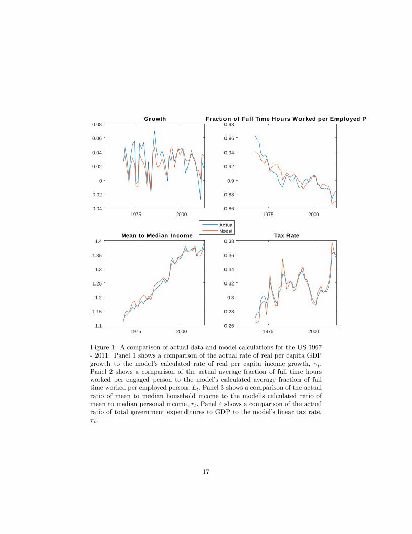
We estimate our model for the United States over two different time periods.During the first period from 1967 to 2011 we use annual observations on realper capita GDP growth rate, average annual hours worked per engaged person,the ratio of mean to median household income, and the burden of governmentwhich is total government expenditures/GDP. During the second, longer periodwe substitute the income share of the top 10% for the ratio of mean to medianhousehold income which is not available prior to 1967.We begin with data from the US from 1967 - 2011. Figure 1 shows a
comparison of actual data and model calculations. Obviously the fits of themodel to the data are excellent. The r2 for the fit of actual data to themodel are 55.4%, 77.6%, 98.1%, and 86.5%, for growth, hours per employedperson, mean to median income, and the tax rate, respectively. The downwardtrend in hours worked per employed person reflects an international trend aswe see below. Mean to median income and government expenditures as afraction of GDP have both trended upward as a result of increased dispersionin productivity as shown in Figure 2.Figure 2 shows the optimal estimated states, {gt, σt, wt}, and νt, from 1967
- 2011. The productivity growth multiplier, shown in Panel 1, increased from1967, reached a peak in 2000, and declined afterward. The dispersion of relativeproductivity, shown in Panel 2, increased steadily from 1967 through 2000, buthas leveled off since then. In contrast to the other state variables, wt growsthroughout the sample, reflecting the continuous growth in US productivity.There has been a steady upward trend in the productivity cutoff for voluntaryunemployment.
16
1975 20000.04
0.02
0
0.02
0.04
0.06
0.08Growth
ActualModel
1975 20000.86
0.88
0.9
0.92
0.94
0.96
0.98Fraction of Full Time Hours Worked per Employed Person
1975 20001.1
1.15
1.2
1.25
1.3
1.35
1.4Mean to Median Income
1975 20000.26
0.28
0.3
0.32
0.34
0.36
0.38Tax Rate
Figure 1: A comparison of actual data and model calculations for the US 1967- 2011. Panel 1 shows a comparison of the actual rate of real per capita GDPgrowth to the model’s calculated rate of real per capita income growth, γt.Panel 2 shows a comparison of the actual average fraction of full time hoursworked per engaged person to the model’s calculated average fraction of fulltime worked per employed person, Lt. Panel 3 shows a comparison of the actualratio of mean to median household income to the model’s calculated ratio ofmean to median personal income, rt. Panel 4 shows a comparison of the actualratio of total government expenditures to GDP to the model’s linear tax rate,τ t.
17

1975 20000.005
0.01
0.015
0.02
0.025
0.03G
1975 20000.45
0.5
0.55
0.6
0.65
0.7
0.75
0.8Sigma
1975 20000.5
1
1.5
2
2.5W
MeanMedian
1975 20000.05
0.06
0.07
0.08
0.09
0.1
0.11Nu
Figure 2: Estimated state variables in the US from 1967 - 2011. The firstpanel shows the productivity growth multiplier. The second panel show thestandard deviation or dispersion of productivity. The third panel shows theabsolute productivity index for the median worker; also, for comparison, is themean productivity index as computed by the BLS. The fourth panel shows theproductivity of the last person who voluntarily chooses not to work.
18
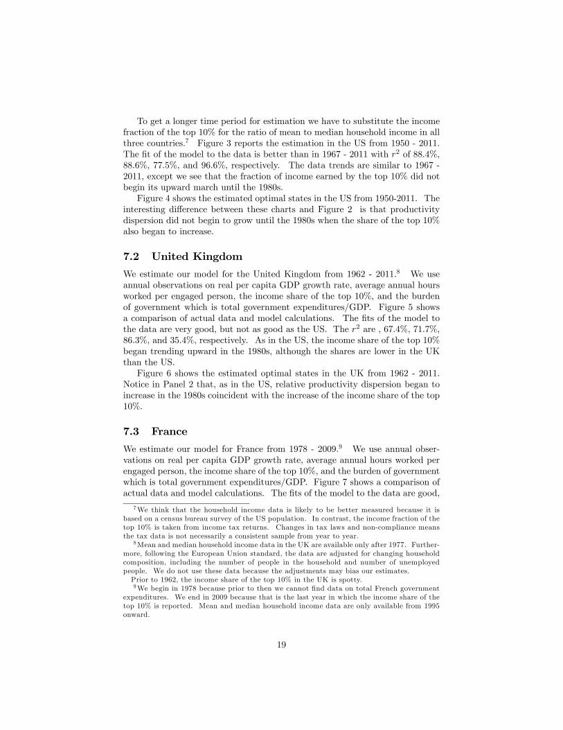
To get a longer time period for estimation we have to substitute the incomefraction of the top 10% for the ratio of mean to median household income in allthree countries.7 Figure 3 reports the estimation in the US from 1950 - 2011.The fit of the model to the data is better than in 1967 - 2011 with r2 of 88.4%,88.6%, 77.5%, and 96.6%, respectively. The data trends are similar to 1967 -2011, except we see that the fraction of income earned by the top 10% did notbegin its upward march until the 1980s.Figure 4 shows the estimated optimal states in the US from 1950-2011. The
interesting difference between these charts and Figure 2 is that productivitydispersion did not begin to grow until the 1980s when the share of the top 10%also began to increase.
7.2 United Kingdom
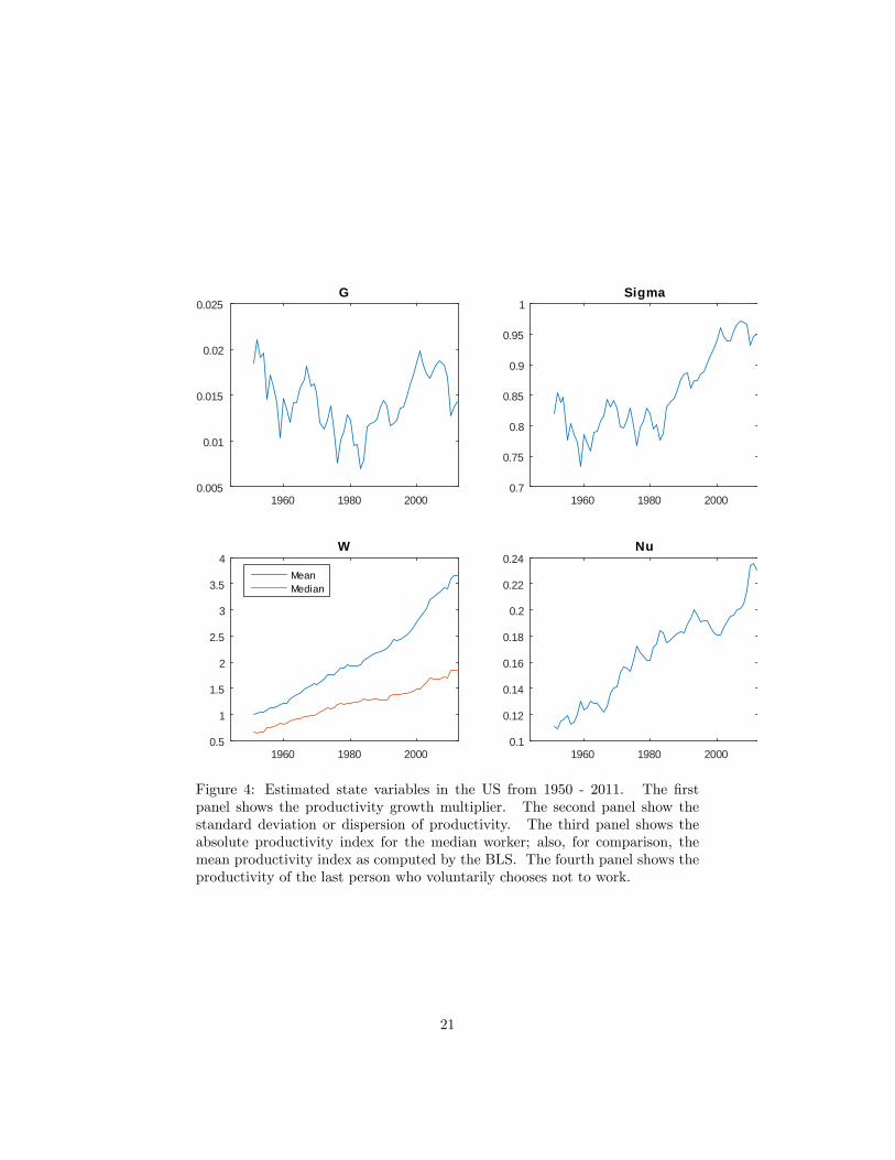
We estimate our model for the United Kingdom from 1962 - 2011.8 We useannual observations on real per capita GDP growth rate, average annual hoursworked per engaged person, the income share of the top 10%, and the burdenof government which is total government expenditures/GDP. Figure 5 showsa comparison of actual data and model calculations. The fits of the model tothe data are very good, but not as good as the US. The r2 are , 67.4%, 71.7%,86.3%, and 35.4%, respectively. As in the US, the income share of the top 10%began trending upward in the 1980s, although the shares are lower in the UKthan the US.Figure 6 shows the estimated optimal states in the UK from 1962 - 2011.
Notice in Panel 2 that, as in the US, relative productivity dispersion began toincrease in the 1980s coincident with the increase of the income share of the top10%.
7.3 France
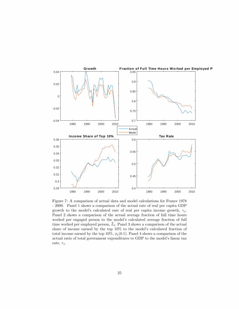
We estimate our model for France from 1978 - 2009.9 We use annual obser-vations on real per capita GDP growth rate, average annual hours worked perengaged person, the income share of the top 10%, and the burden of governmentwhich is total government expenditures/GDP. Figure 7 shows a comparison ofactual data and model calculations. The fits of the model to the data are good,
7We think that the household income data is likely to be better measured because it isbased on a census bureau survey of the US population. In contrast, the income fraction of thetop 10% is taken from income tax returns. Changes in tax laws and non-compliance meansthe tax data is not necessarily a consistent sample from year to year.
8Mean and median household income data in the UK are available only after 1977. Further-more, following the European Union standard, the data are adjusted for changing householdcomposition, including the number of people in the household and number of unemployedpeople. We do not use these data because the adjustments may bias our estimates.Prior to 1962, the income share of the top 10% in the UK is spotty.9We begin in 1978 because prior to then we cannot find data on total French government
expenditures. We end in 2009 because that is the last year in which the income share of thetop 10% is reported. Mean and median household income data are only available from 1995onward.
19

1960 1980 20000.06
0.04
0.02
0
0.02
0.04
0.06
0.08Growth
ActualModel
1960 1980 20000.7
0.75
0.8
0.85Fraction of Full Time Hours Worked per Employed Person
1960 1980 20000.3
0.35
0.4
0.45
0.5Income Share of Top 10%
1960 1980 20000.2
0.25
0.3
0.35
0.4Tax Rate
Figure 3: A comparison of actual data and model calculations for the US 1950- 2011. Panel 1 shows a comparison of the actual rate of real per capita GDPgrowth to the model’s calculated rate of real per capita income growth, γt.Panel 2 shows a comparison of the actual average fraction of full time hoursworked per engaged person to the model’s calculated average fraction of fulltime worked per employed person, Lt. Panel 3 shows a comparison of the actualshare of income earned by the top 10% to the model’s calculated fraction oftotal income earned by the top 10%, φt(0.1). Panel 4 shows a comparison of theactual ratio of total government expenditures to GDP to the model’s linear taxrate, τ t.
20
1960 1980 20000.005
0.01
0.015
0.02
0.025G
1960 1980 20000.7
0.75
0.8
0.85
0.9
0.95
1Sigma
1960 1980 20000.5
1
1.5
2
2.5
3
3.5
4W
MeanMedian
1960 1980 20000.1
0.12
0.14
0.16
0.18
0.2
0.22
0.24Nu
Figure 4: Estimated state variables in the US from 1950 - 2011. The firstpanel shows the productivity growth multiplier. The second panel show thestandard deviation or dispersion of productivity. The third panel shows theabsolute productivity index for the median worker; also, for comparison, themean productivity index as computed by the BLS. The fourth panel shows theproductivity of the last person who voluntarily chooses not to work.
21

1975 20000.06
0.04
0.02
0
0.02
0.04
0.06
0.08Growth
ActualModel
1975 20000.65
0.7
0.75
0.8
0.85
0.9
0.95Fraction of Full Time Hours Worked per Employed Person
1975 20000.25
0.3
0.35
0.4
0.45Income Share of Top 10%
1975 20000.3
0.35
0.4
0.45
0.5Tax Rate
Figure 5: A comparison of actual data and model calculations for the UK 1962- 2011. Panel 1 shows a comparison of the actual rate of real per capita GDPgrowth to the model’s calculated rate of real per capita income growth, γt.Panel 2 shows a comparison of the actual average fraction of full time hoursworked per engaged person to the model’s calculated average fraction of fulltime worked per employed person, Lt. Panel 3 shows a comparison of the actualshare of income earned by the top 10% to the model’s calculated fraction oftotal income earned by the top 10%, φt(0.1). Panel 4 shows a comparison of theactual ratio of total government expenditures to GDP to the model’s linear taxrate, τ t.
22
1975 2000
10 3
5
0
5
10
15
20G
1975 20000.6
0.7
0.8
0.9
1Sigma
1975 20000
1
2
3
4
5
6W
MeanMedian
1975 20000.1
0.15
0.2
0.25
0.3Nu
Figure 6: Estimated state variables in the UK from 1962 - 2011. The firstpanel shows the productivity growth multiplier. The second panel show thestandard deviation or dispersion of productivity. The third panel shows theabsolute productivity index for the median worker; also, for comparison, themean productivity index as computed by the BLS. The fourth panel shows theproductivity of the last person who voluntarily chooses not to work.
23

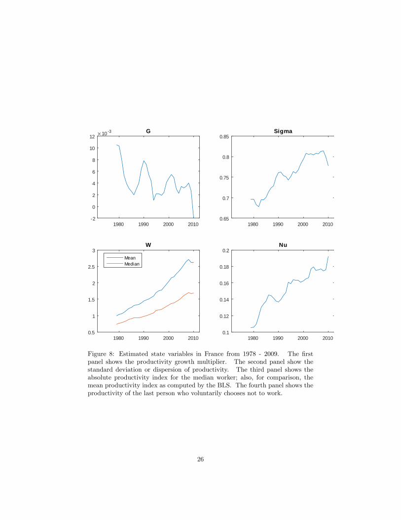
but not as good as the US or UK. The r2 are 60.2%, 80.2%, -70.7%, and 79.5%,respectively. The fit of the model to the actual income share of the top 10% ispoor; since 1995 the model requires a larger share for the top 10% than the taxdata shows.Figure 8 shows the estimated optimal states in France from 1978 - 2009.
Notice in Panel 2 that, as in the US and UK, relative productivity dispersionbegan to increase in the 1980s coincident with the increase of the income shareof the top 10%.
7.4 Technological Specialization and the Dispersion of Pro-ductivity
In all three countries, an important cause for the change in the distribution ofproductivity is technological specialization. New technologies result in diver-gent growth in productivity, which increase σt. Increased returns to special-ization cause the distribution of relative productivity to widen. Evidently, asshown in Panel 2 of Figures 2, 4, 6, and 8, there has been a significant widen-ing in the dispersion of relative productivity, σt, in the U.S., UK and France,respectively. This dispersion has been attributed to the growth of computertechnology.10 Those who are able to lever their skills through technologyhave become relatively more productive in comparison with the median worker.This technological change has increased the growth rate of the economy and thedispersion of pre-tax income.
7.5 Statistics
We compute the model parameters by minimizing the sum of squared errorswhich is equivalent to maximizing the likelihood. Hence we can find the stan-dard errors of the model parameters using the outer product of gradients esti-mator. The two unknown parameters in each country are the number of annualhours comprising full time work, Λ, and the maximum fraction of time devotedto work, λ.
10See Gordon (2002). More recently Gordon and Mokyr have joined in a lively debate overwhether continued technological change will fuel future productivity growth Aeppel (2014).
24
1980 1990 2000 20100.04
0.02
0
0.02
0.04Growth
ActualModel
1980 1990 2000 20100.7
0.75
0.8
0.85
0.9
0.95Fraction of Full Time Hours Worked per Employed Person
1980 1990 2000 20100.29
0.3
0.31
0.32
0.33
0.34
0.35
0.36Income Share of Top 10%
1980 1990 2000 20100.4
0.45
0.5
0.55
0.6Tax Rate
Figure 7: A comparison of actual data and model calculations for France 1978- 2009. Panel 1 shows a comparison of the actual rate of real per capita GDPgrowth to the model’s calculated rate of real per capita income growth, γt.Panel 2 shows a comparison of the actual average fraction of full time hoursworked per engaged person to the model’s calculated average fraction of fulltime worked per employed person, Lt. Panel 3 shows a comparison of the actualshare of income earned by the top 10% to the model’s calculated fraction oftotal income earned by the top 10%, φt(0.1). Panel 4 shows a comparison of theactual ratio of total government expenditures to GDP to the model’s linear taxrate, τ t.
25
1980 1990 2000 2010
10 3
2
0
2
4
6
8
10
12G
1980 1990 2000 20100.65
0.7
0.75
0.8
0.85Sigma
1980 1990 2000 20100.5
1
1.5
2
2.5
3W
MeanMedian
1980 1990 2000 20100.1
0.12
0.14
0.16
0.18
0.2Nu
Figure 8: Estimated state variables in France from 1978 - 2009. The firstpanel shows the productivity growth multiplier. The second panel show thestandard deviation or dispersion of productivity. The third panel shows theabsolute productivity index for the median worker; also, for comparison, themean productivity index as computed by the BLS. The fourth panel shows theproductivity of the last person who voluntarily chooses not to work.
26

λ ΛUS 1967 - 2011 0.86 1925
(97) (187)US 1950 - 2011 0.69 2264
(21) (55)UK 1962 - 2011 0.78 2404
(16) (25)FR 1978 - 2009 0.88 1999
(64) (52)
Table 3: Estimated model parameters and their T-statstics.The estimates areasymptotically consistent.
Our estimated parameters are shown in Table 3. The estimated full timeannual hours worked (λΛ) ranges from 1562 in the US from 1950 - 2011 to 1875in the UK from 1962 - 2011.
8 Conclusion
Our contribution to the large and very diverse literature on growth and incomedistribution takes the form of a general equilibrium model of growth in laborincome and consumption. The tax rate, as measured by the total governmentburden, and the amount spent on redistribution are endogenous variables. Indeveloped, democratic countries voters chose the tax rate in single issue elec-tions. The budget is balanced, so spending and tax collections are equal. Byassumption, all spending is for redistribution.The model extends our earlier work on a static economy, Meltzer and Richard (1981),
to a growing economy. Consumers are endowed with different initial levels ofproductivity. Output and labor income change, as does productivity and, withit, the distribution of income among income groups. In our model, labor pro-ductivity changes as workers learn more productive skills on the job and astechnology changes. This changes relative and absolute incomes and the spreadbetween the top and the bottom (or other aspects) of the income distribution.Our model analyzes consumption over time. Consumption is an endogenous
variable that depends, inter alia, on taxation. Voters choose the tax rate inperiodic elections. Sometimes they choose to increase current consumption byincreasing tax rates and redistribution. Since higher tax rates reduce investmentin learning by doing, the growth rate falls. Voters can vote to increase growthby subsequently voting to reduce tax rates to increase future consumption. Thespread between top and bottom of the income distribution declines. Estimationof the model shows good correspondence to the historical data for the tax rate,average hours worked per employed person, the distribution of pre-tax income,and the growth rate of the economy which means the model captures the mainfacts about redistribution and economic growth.
27

The model answers the puzzling result emphasized by Piketty (2014). Asdid Karl Marx, Piketty concludes that because the return on capital repeatedlyexceeds the growth rate of developed economies and does not change much overtime, developed economies will face ever-increasing capital stocks. Since returnsto capital go mainly to the highest income groups, the distribution of incomewidens over time and will continue to do so. Another possibility, of course, isthat capital owners either consume or donate to charity the capital output inexcess of the economic growth rate, so that capital does not accumulate fasterthan the economy grows. The puzzle for Piketty’s conjecture is why there isno evidence anywhere that the capital stock has approached saturation. Thatfact opens the way for an alternative explanation of the relative constancy ofthe return to capital. Unlike Piketty who bases his conclusion on a comparisonof the before tax income of the top 1 or 0.1 percent to before redistribution tothe lowest income groups, we compare incomes available for consumption by thedifferent income classes. Piketty’s choice greatly overstates what has happenedin developed countries. Our measure is more closely related to income aftertax and after redistribution, hence to consumption. In our model, labor isthe source of income. Unlike the return to capital, the return to labor hasincreased considerably over time. It is subject to cyclical and other changesin relative share. And it changes with productivity growth, thereby increasingat times the relative shares of those in the working classes while reducing theirrelative share in periods of low growth, and therefore consumption. As Kuznetsconjectured, we must look to changes in labor income to explain changes in thespread between high and low income shares. Data for the three countries westudy support our model and the Kuznets’conjecture.
References
Acemoglu, Daron (2009). Introduction to Modern Economic Growth. Prince-ton: Princeton University Press.
Aeppel, Timothy, (2014). "Economists Debate: Has All the Important StuffAlready Been Invented?", The Wall St. Journal, June 14, 2014.
Alesina, Alberto and Rodrik, Dani, (1994). “Distributive Politics and EconomicGrowth,”Quarterly Journal of Economics, 109, 2, May, 465-90.
Autor, David H., (2014). "Skills, education and the rise of earning inequalityamong the ’other 99 percent’," Science, 344, May, 844-51.
Becker, Gary S. and Tomes, Nigel, (1979). “An Equilibrium Theory of the Distri-bution of Income and Intergenerational Mobility,”Journal of Political Econ-omy, 87, 6, 1153-89.
Becker, Gary S. and Tomes, Nigel, (1986). “Human Capital and the Rise andFall of Families,”Journal of Labor Economics, 4, 3, Part 2, July 51-539.
28

Corak, Miles, (2013). “Income Inequality, Equality of Opportunity, and Inter-generational Mobility,” Journal of Economic Perspectives, 27, 3, Summer,79-102.
Gordon, Robert J., (2002). Technology and Economic Performance in the Amer-ican Economy, NBER, February, 2002.
Kaplan, Steven N. and Rauh, Joshua, (2013). “It’s the Market: The Broad-Based Rise in the Return to Top Talent,”Journal of Economic Perspectives,27, 3, Summer, 35-56.
Kuznets, Simon, (1955). “Economic Growth and Income Inequality,”AmericanEconomic Review, 45, 1, 1-28.
Kuznets, Simon, (1979). Growth, Population and Income Distribution: SelectedEssays, New York: W.W. Norton.
Meltzer, Allan H. and Richard, Scott, F., (1981). “A Rational Theory of theSize of Government,”Journal of Political Economy, 89, 5, 914-27.
Okun, Arthur, (1975). Equality and Effi ciency: The Big Tradeoff, Washington:Brookings.
Perri, Fabrizio, (2014). “Inequality,”Annual Report, Federal Reserve Bank ofMinneapolis, 5-27.
Piguillem, Facundo and Anderson L. Schneider (2013). "Heterogeneous Laborskills, the Median voter and Labor Taxes," Review of Economics Dynamics,16, April 2013, 332-349.
Piketty, Thomas, (2014). Capital in the Twenty-First Century, translated byArthur Goldhammner, Cambridge, MA., Belknap Press.
Roberts, Kevin W. S., (1977). "Voting Over Income Tax Schedules," Journal ofPublic Economics, 8, (December 1977), 329-40.
Romer, Thomas, (1975). "Individual welfare, majority voting, and the proper-ties of a linear income tax," Journal of Public Economics, 4, February 1975,163-185.
Roine, Joseph and Waldenstrom, Daniel, (2006). “The Evolution of Incomes inan Egalitarian Society: Sweden 1903-2004,”Stockholm School of Economics.
Rosen, Sherwin, (1981). “The Economics of Superstars,”American EconomicReview, 71, 5, 845-58.
Saez, Emanuel, (2013). “Income Inequality: Evidence and Policy Implications,”Arrow Lecture, Stanford University, January.
29