A Parallel Feature Selection Algorithm fromRandom Subsets

Daniel J. Garcia, Lawrence O. Hall, Dmitry B. Goldgof, and Kurt Kramer

Department of Computer Science and Engineering4202 E. Fowler Ave. ENB118University of South Florida

Tampa, FL 33620, USA(djgarcia,hall,goldgof,kkramer)@csee.usf.edu

Abstract. Feature selection methods are used to find the set of featuresthat yield the best classification accuracy for a given data set. This re-sults in lower training and classification time for a classifier, a supportvector machine here, and better classification accuracy. Feature selection,however, may be a time consuming process unfit for real time applica-tion. In this paper, we explore a feature selection algorithm based onsupport vector machine training time. It is compared with the Wrap-per algorithm. Our approach can be run on all available processors inparallel. Our feature selection approach is ideal if new features need tobe selected during data acquisition, where a fast, approximate approachmay be advantageous. Experimental results indicate that the trainingtime based method yields feature sets almost as good as the Wrappermethod, while requiring considerably less computation time.

Keywords: Feature Selection, Parallelism, Random Subsets, Wrappers, SVM.

1 Introduction

Support vector machines (SVMs)[1] are learning algorithms which result in amodel that can be used to classify data. The details of the inner workings ofSVMs are beyond the scope of this paper. For our purposes, SVMs use labeleddata to construct a classifier, and then use it to classify unknown data. In thispaper, the data being analyzed are plankton images obtained from a device calledSIPPER (Shadow Image Particle Profiling Evaluation Recorder) [2]. In orderfor a support vector machine to be able to classify these images, features areextracted from them. These features are used by the SVM to create the supportpoints that will differentiate between images. These features can be numerousand include characteristics such as height, weight, shape, length, transparency,and texture.

The use of all the available features does not guarantee the best accuracy,training, and classification time. It is possible for a subset of features to havebetter accuracy, training, and classification time. Also of importance is the fact

2

that the process of training a SVM is faster if fewer features are used. It is for thisreason that feature selection processes are necessary in order to effectively traina classifier. Feature selection is the process through which an ”optimal” group offeatures for a given data set is found. This process may be a time consuming one,and is typically not well suited for real time applications. The goal is to createa feature selection algorithm that is able to complete its execution in a shortenough amount of time to allow it to be implemented in the field during dataacquisition, while retaining high classification accuracy. Our hypothesis is thatsets of features which result in faster SVM training times can be exploited tocreate overall feature sets which can be used to build a high accuracy classifier.It is expected that less training time will be required to find the boundaries withfeatures that will enable higher accuracy classifiers to be built.

There are many feature selection methods. In fact, there are a number whichare relatively specific for support vector machines [3, 4]. The recursive featureelimination approach has been used with success with SVM’s [4]. Space limita-tions prevent us from doing detailed comparisons, but we do present an alterna-tive, feature selection approach that works with SVM’s.

2 Random Feature Selection

Feature selection methods are applied to all the features describing a data set tofind a subset of features that best describe that data set. The feature selectionmethod proposed in this paper can be divided into two stages. The first stageconsists of generating a number of feature sets of fixed size, then running a 10fold cross validation using only the features found in these sets, to determinehow well they are able to classify the data. It is important to emphasize thatthe features in these sets are randomly selected out of the pool of all features,and thus these sets are generated in a very short amount of time. The sets offeatures are then sorted by a given criteria, such as training time (here) or thenumber of support vectors generated, and the best of these randomly generatedsets are selected for the second stage of the algorithm.

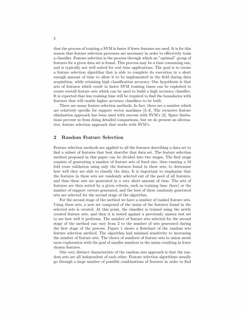
For the second stage of the method we have a number of ranked feature sets.Using these sets, a new set composed of the union of the features found in theselected sets is created. At this point, the classifier is trained using the newlycreated feature sets, and then it is tested against a previously unseen test setto see how well it performs. The number of feature sets selected for the secondstage of the method can vary from 2 to the number of sets generated duringthe first stage of the process. Figure 1 shows a flowchart of the random setsfeature selection method. The algorithm had minimal sensitivity to increasingthe number of feature sets. The choice of numbers of feature sets to union needsmore exploration with the goal of smaller numbers in the union resulting in fewerchosen features.

One very distinct characteristic of the random sets approach is that the ran-dom sets are all independent of each other. Feature selection algorithms usuallygo through a large number of possible combinations of features in order to find

3

Fig. 1. Random Sets Flow Chart

the best one. However, since the number of features could possibly reach thehundreds, the number of possible combinations grows at a very fast rate. Itis for this reason that existing feature selection algorithms do not search forpossible combinations blindly, instead they do it intelligently. This means thatthere is some logic guiding the search, and the next step in the search processis partly based on previous steps. The implications of this characteristic is thatthese feature selection methods cannot fully take advantage of parallel process-ing because future steps in the process need to wait for previous steps to finish.The random sets method, on the other hand, does allow parallel processing. Therandom feature sets created are completely independent from each other, and allof them are evaluated during the same step in the algorithm. For this reason, itis possible for every single random set created to be evaluated in parallel; greatlyreducing the time it takes for this feature selection method to finish its task. Inthis work, timings are reported with all training done on 1 processor. One coulddivide by approximately the number of random feature sets evaluated (there willbe some overhead) to look at the parallel computing time advantage. The readerwill see the speed-ups are quite impressive even without parallelism.

3 Wrappers

An alternative algorithm for feature selection is also presented. Feature selectionmethods usually work by trying combinations of features from the original poolof features and then choosing the combination that yields the best results. Onesuch method consists of organizing the feature combinations in a tree structure.In this organization, the nodes of the tree are simply a given combination offeatures. This is the approach taken by the Wrapper feature selection method [5].

4

A given combination of features is passed to a learning algorithm for evaluationand then the results are obtained and kept for later comparison. The results fromthe learning algorithm are then used to intelligently search the tree structure.

To illustrate this approach, let us assume we have n features. The root ofthe tree is the set containing all n features. This set is analyzed first and theaccuracy is stored. The next step in the algorithm is to choose the best storedresults and then analyze every combination of the number of features in that setminus one. In the current case, only the results of analyzing one set have beenobtained, so the next step would be to analyze every combination of n -1 featuresand store the results. At this point, a best first search is done, which means thatthe best case, gauged by the classification accuracy, is selected in order to repeatthe process of searching for every combination of features of length s - 1, wheres is the number of features in the most recently selected feature set. Thus, thenext step is to look at all (n - 1) - 1 = n - 2 subsets of the best n - 1 grouping.

The stopping criterion was the analysis of a fixed number of new featuresets without finding a new set with clearly higher accuracy [6]. We did allowsub-optimal (5th best) sets to be examined with a low probability.

This feature selection method can’t take full advantage of parallel processing.This is so because the search has to wait for the results of all the processedcombinations before it can select the best next case. Suppose combinations ofsize s are being analyzed, all of these combinations come from a parent of size s+ 1. Theoretically, every combination of size s in this case can be processed atthe same time if enough processors are present. However, the result from thesesets will be considered for the next best case, which forces this method to waituntil every set of size s is evaluated before it can continue.

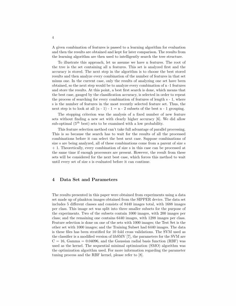
4 Data Set and Parameters

The results presented in this paper were obtained from experiments using a dataset made up of plankton images obtained from the SIPPER device. The data setincludes 5 different classes and consists of 8440 images total, with 1688 imagesper class. This image set was split into three smaller subsets for the purpose ofthe experiments. Two of the subsets contain 1000 images, with 200 images perclass; and the remaining one contains 6440 images, with 1288 images per class.Feature selection is done on one of the sets with 1000 images; the Test Set is theother set with 1000 images; and the Training Subset had 6440 images. The datais these files has been stratified for 10 fold cross validations. The SVM used asthe classifier is a modified version of libSMV [7], the parameters for the SVM areC = 16, Gamma = 0.04096, and the Gaussian radial basis function (RBF) wasused as the kernel. The sequential minimal optimization (SMO) algorithm wasthe optimization algorithm used. For more information regarding the parametertuning process and the RBF kernel, please refer to [8].

5

5 Experiments and Results

The procedure for the experiments was the following. First, from the originalpool of 47 features extracted from the plankton images, 200 random subsetswith 10 features each were created. We did some empirical tests and found thesenumbers to be the best of a range of reasonably equivalent choices. Clearly, theselection will make a difference.

A ten fold cross validation was done on the Feature Selection data set usingeach one of these sets independently, and the time it took to train the SVM usingthese sets was recorded. Next, the 9 feature sets associated with the shortesttraining times were selected for the second stage of our method. Three new setswere created by using the union of the features found in the selected sets: theunion of the 3 sets, the union of the 5 sets, and the union of the 9 sets, respectivelyassociated with the ordered shortest training time. Finally, the Feature Selectiondata set and the Training Subset data set are put together into a joint data setand a classifier is trained on this joint set using the three new feature sets. Thenthe classifier is tested against the unseen Test Set to obtain the final results.

The whole procedure is repeated five times with five different randomly cho-sen stratified sets of data. The results reported are the average values of the fiveexperiments.

For the Wrapper approach, the procedure was the following. First, a searchwas performed on the Feature Selection set using a 5 fold cross validation toevaluate the feature sets. This will yield an accuracy value for each level in thesearch tree, thus we get an accuracy value for the best sets of n features, wheren goes from 1 feature to all features. Next, the union of the Training Subsetand the Feature Selection set are used to train the classifier using the best setof features at a specific level in the tree, and then the classifier is tested againstthe Test Set to determine how accurate it is on unseen data.

As with the random sets approach, this whole procedure is repeated five timesover the same data sets as the random sets method and the results reported arethe average values of the five different experiments.

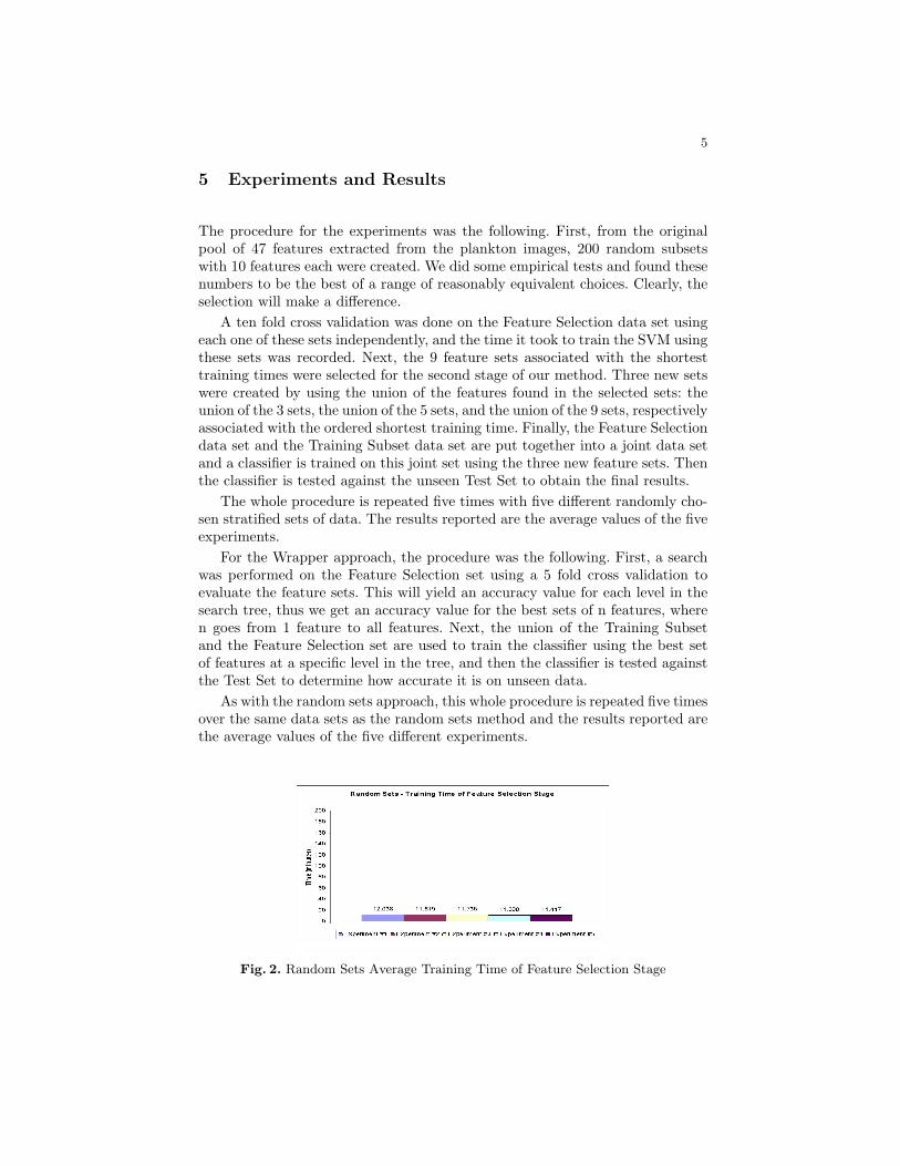
Fig. 2. Random Sets Average Training Time of Feature Selection Stage

6

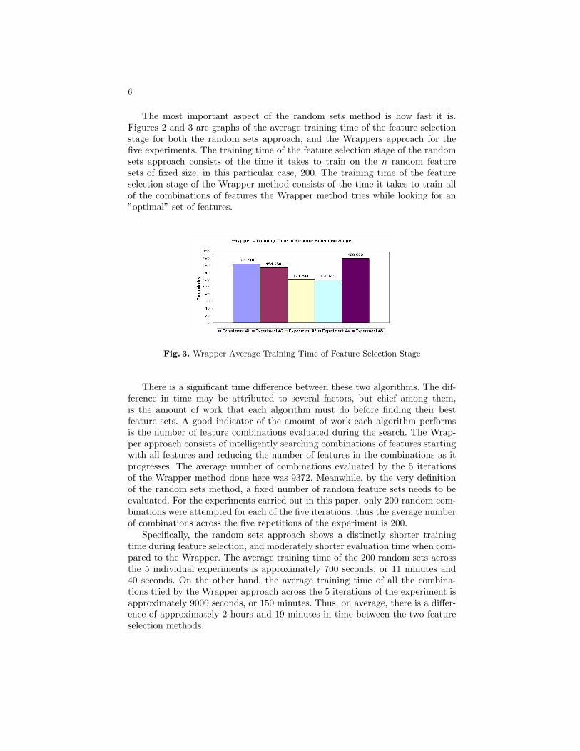
The most important aspect of the random sets method is how fast it is.Figures 2 and 3 are graphs of the average training time of the feature selectionstage for both the random sets approach, and the Wrappers approach for thefive experiments. The training time of the feature selection stage of the randomsets approach consists of the time it takes to train on the n random featuresets of fixed size, in this particular case, 200. The training time of the featureselection stage of the Wrapper method consists of the time it takes to train allof the combinations of features the Wrapper method tries while looking for an”optimal” set of features.

Fig. 3. Wrapper Average Training Time of Feature Selection Stage

There is a significant time difference between these two algorithms. The dif-ference in time may be attributed to several factors, but chief among them,is the amount of work that each algorithm must do before finding their bestfeature sets. A good indicator of the amount of work each algorithm performsis the number of feature combinations evaluated during the search. The Wrap-per approach consists of intelligently searching combinations of features startingwith all features and reducing the number of features in the combinations as itprogresses. The average number of combinations evaluated by the 5 iterationsof the Wrapper method done here was 9372. Meanwhile, by the very definitionof the random sets method, a fixed number of random feature sets needs to beevaluated. For the experiments carried out in this paper, only 200 random com-binations were attempted for each of the five iterations, thus the average numberof combinations across the five repetitions of the experiment is 200.

Specifically, the random sets approach shows a distinctly shorter trainingtime during feature selection, and moderately shorter evaluation time when com-pared to the Wrapper. The average training time of the 200 random sets acrossthe 5 individual experiments is approximately 700 seconds, or 11 minutes and40 seconds. On the other hand, the average training time of all the combina-tions tried by the Wrapper approach across the 5 iterations of the experiment isapproximately 9000 seconds, or 150 minutes. Thus, on average, there is a differ-ence of approximately 2 hours and 19 minutes in time between the two featureselection methods.

7

The difference in evaluation time is not as great as the difference betweenthe training times. Across the 5 experiments, the average evaluation time forthe 200 randomly created sets is 43 seconds. The Wrapper, on the other hand,spent on average 2498 seconds, or 41 minutes and 38 seconds, on evaluation time.Adding the training time and the evaluation time together we get the total CPUtime spent on each method. The random sets method spent an average of 744seconds, or roughly 12 minutes to complete; on the other hand, the Wrappermethod spent an average of 11,431 seconds, roughly 191 minutes, or 3 hours and11 minutes, to finish.

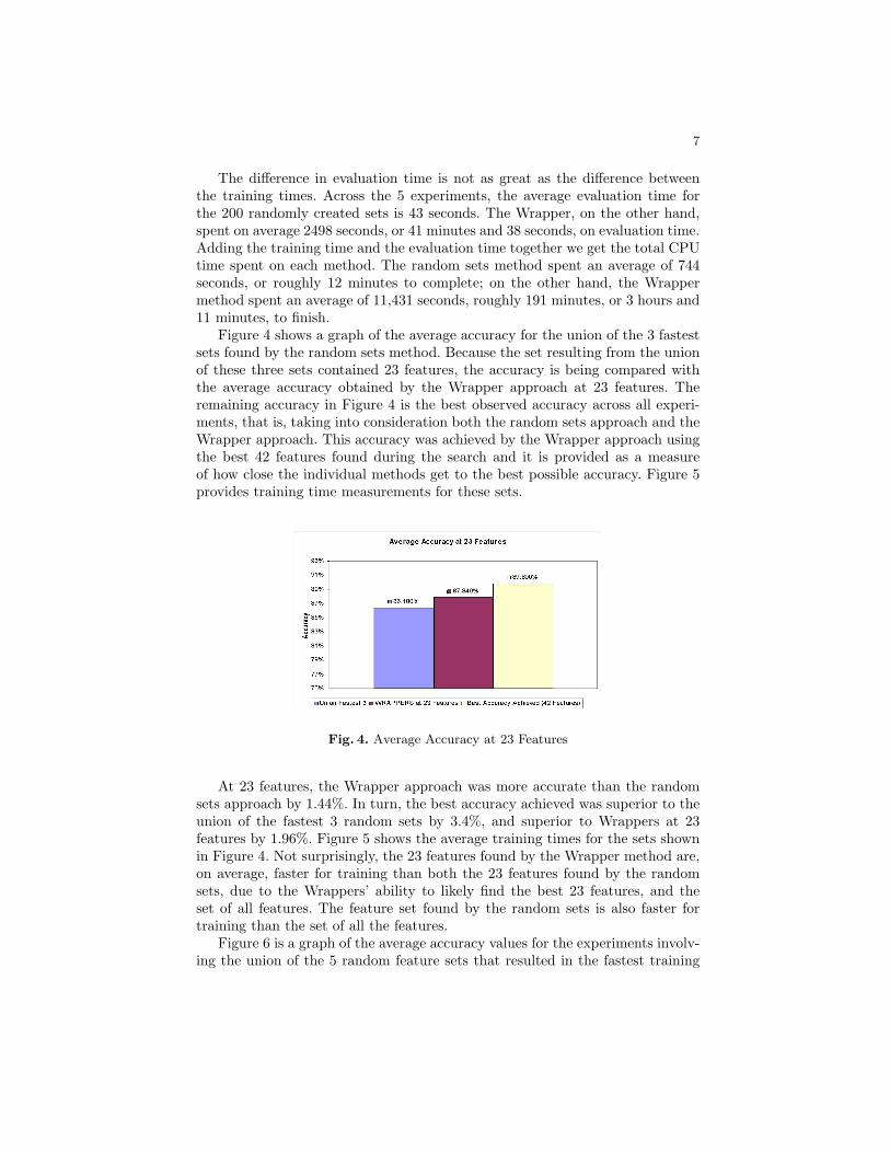
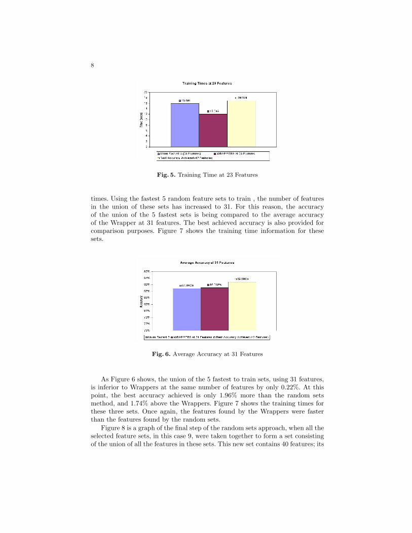
Figure 4 shows a graph of the average accuracy for the union of the 3 fastestsets found by the random sets method. Because the set resulting from the unionof these three sets contained 23 features, the accuracy is being compared withthe average accuracy obtained by the Wrapper approach at 23 features. Theremaining accuracy in Figure 4 is the best observed accuracy across all experi-ments, that is, taking into consideration both the random sets approach and theWrapper approach. This accuracy was achieved by the Wrapper approach usingthe best 42 features found during the search and it is provided as a measureof how close the individual methods get to the best possible accuracy. Figure 5provides training time measurements for these sets.

Fig. 4. Average Accuracy at 23 Features

At 23 features, the Wrapper approach was more accurate than the randomsets approach by 1.44%. In turn, the best accuracy achieved was superior to theunion of the fastest 3 random sets by 3.4%, and superior to Wrappers at 23features by 1.96%. Figure 5 shows the average training times for the sets shownin Figure 4. Not surprisingly, the 23 features found by the Wrapper method are,on average, faster for training than both the 23 features found by the randomsets, due to the Wrappers’ ability to likely find the best 23 features, and theset of all features. The feature set found by the random sets is also faster fortraining than the set of all the features.

Figure 6 is a graph of the average accuracy values for the experiments involv-ing the union of the 5 random feature sets that resulted in the fastest training

8

Fig. 5. Training Time at 23 Features

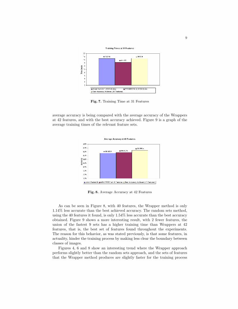
times. Using the fastest 5 random feature sets to train , the number of featuresin the union of these sets has increased to 31. For this reason, the accuracyof the union of the 5 fastest sets is being compared to the average accuracyof the Wrapper at 31 features. The best achieved accuracy is also provided forcomparison purposes. Figure 7 shows the training time information for thesesets.

Fig. 6. Average Accuracy at 31 Features

As Figure 6 shows, the union of the 5 fastest to train sets, using 31 features,is inferior to Wrappers at the same number of features by only 0.22%. At thispoint, the best accuracy achieved is only 1.96% more than the random setsmethod, and 1.74% above the Wrappers. Figure 7 shows the training times forthese three sets. Once again, the features found by the Wrappers were fasterthan the features found by the random sets.

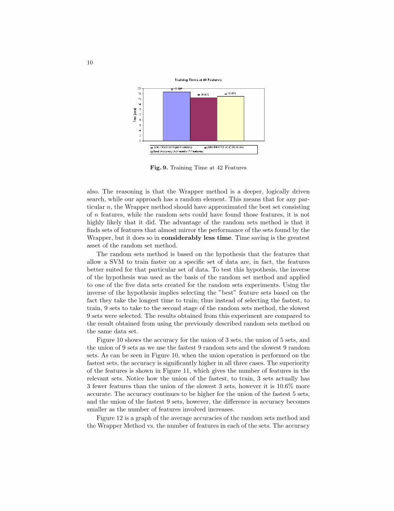
Figure 8 is a graph of the final step of the random sets approach, when all theselected feature sets, in this case 9, were taken together to form a set consistingof the union of all the features in these sets. This new set contains 40 features; its

9

Fig. 7. Training Time at 31 Features

average accuracy is being compared with the average accuracy of the Wrappersat 42 features, and with the best accuracy achieved. Figure 9 is a graph of theaverage training times of the relevant feature sets.

Fig. 8. Average Accuracy at 42 Features

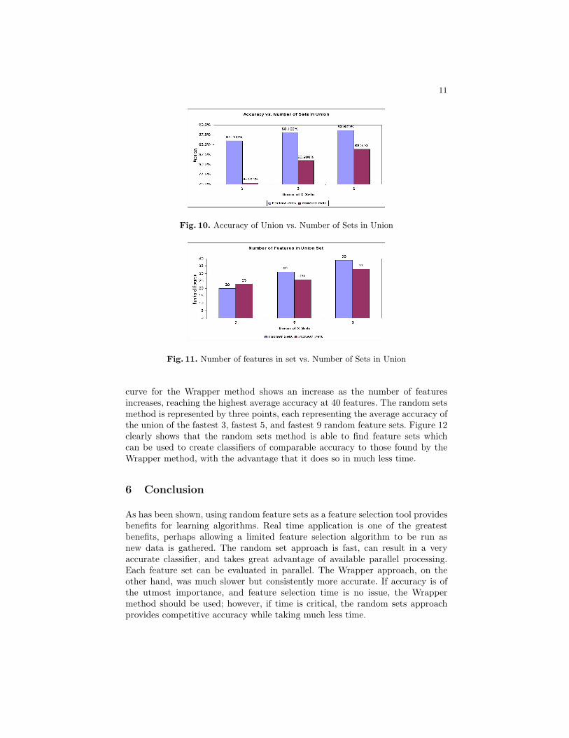
As can be seen in Figure 8, with 40 features, the Wrapper method is only1.14% less accurate than the best achieved accuracy. The random sets method,using the 40 features it found, is only 1.54% less accurate than the best accuracyobtained. Figure 9 shows a more interesting result, with 2 fewer features, theunion of the fastest 9 sets has a higher training time than Wrappers at 42features, that is, the best set of features found throughout the experiments.The reason for this behavior, as was stated previously, is that some features, inactuality, hinder the training process by making less clear the boundary betweenclasses of images.

Figures 4, 6 and 8 show an interesting trend where the Wrapper approachperforms slightly better than the random sets approach, and the sets of featuresthat the Wrapper method produces are slightly faster for the training process

10

Fig. 9. Training Time at 42 Features

also. The reasoning is that the Wrapper method is a deeper, logically drivensearch, while our approach has a random element. This means that for any par-ticular n, the Wrapper method should have approximated the best set consistingof n features, while the random sets could have found those features, it is nothighly likely that it did. The advantage of the random sets method is that itfinds sets of features that almost mirror the performance of the sets found by theWrapper, but it does so in considerably less time. Time saving is the greatestasset of the random set method.

The random sets method is based on the hypothesis that the features thatallow a SVM to train faster on a specific set of data are, in fact, the featuresbetter suited for that particular set of data. To test this hypothesis, the inverseof the hypothesis was used as the basis of the random set method and appliedto one of the five data sets created for the random sets experiments. Using theinverse of the hypothesis implies selecting the ”best” feature sets based on thefact they take the longest time to train; thus instead of selecting the fastest, totrain, 9 sets to take to the second stage of the random sets method, the slowest9 sets were selected. The results obtained from this experiment are compared tothe result obtained from using the previously described random sets method onthe same data set.

Figure 10 shows the accuracy for the union of 3 sets, the union of 5 sets, andthe union of 9 sets as we use the fastest 9 random sets and the slowest 9 randomsets. As can be seen in Figure 10, when the union operation is performed on thefastest sets, the accuracy is significantly higher in all three cases. The superiorityof the features is shown in Figure 11, which gives the number of features in therelevant sets. Notice how the union of the fastest, to train, 3 sets actually has3 fewer features than the union of the slowest 3 sets, however it is 10.6% moreaccurate. The accuracy continues to be higher for the union of the fastest 5 sets,and the union of the fastest 9 sets, however, the difference in accuracy becomessmaller as the number of features involved increases.

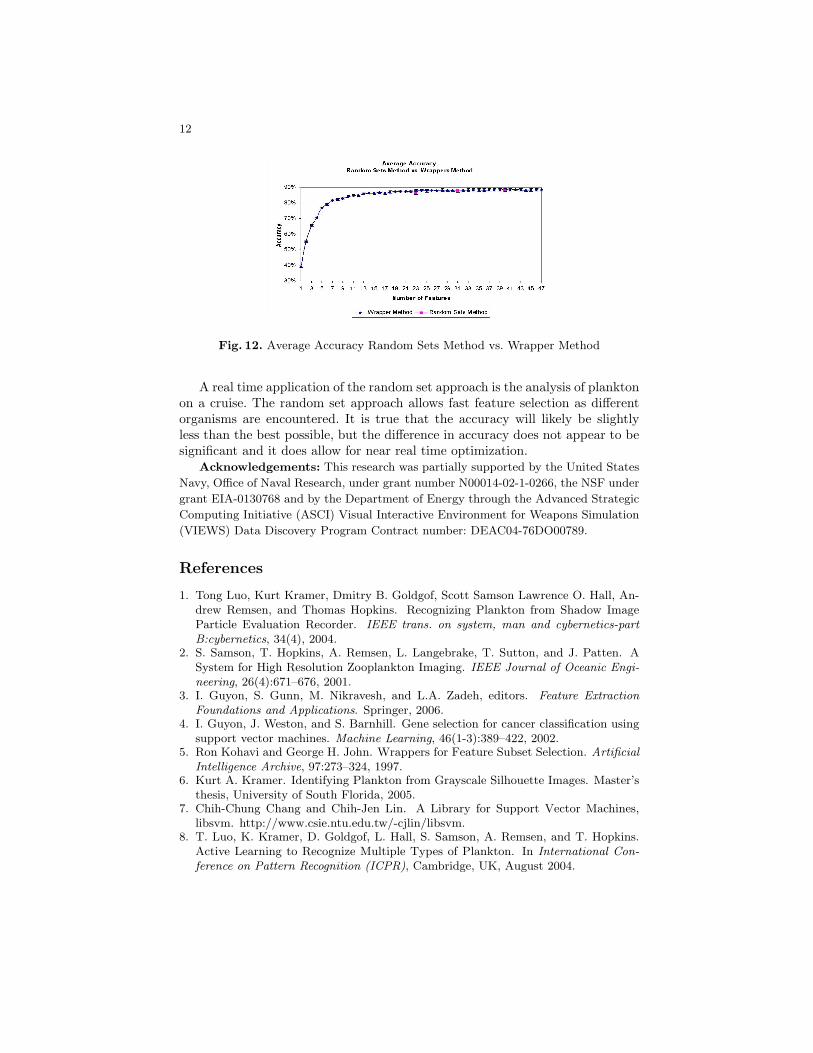
Figure 12 is a graph of the average accuracies of the random sets method andthe Wrapper Method vs. the number of features in each of the sets. The accuracy

11

Fig. 10. Accuracy of Union vs. Number of Sets in Union

Fig. 11. Number of features in set vs. Number of Sets in Union

curve for the Wrapper method shows an increase as the number of featuresincreases, reaching the highest average accuracy at 40 features. The random setsmethod is represented by three points, each representing the average accuracy ofthe union of the fastest 3, fastest 5, and fastest 9 random feature sets. Figure 12clearly shows that the random sets method is able to find feature sets whichcan be used to create classifiers of comparable accuracy to those found by theWrapper method, with the advantage that it does so in much less time.

6 Conclusion

As has been shown, using random feature sets as a feature selection tool providesbenefits for learning algorithms. Real time application is one of the greatestbenefits, perhaps allowing a limited feature selection algorithm to be run asnew data is gathered. The random set approach is fast, can result in a veryaccurate classifier, and takes great advantage of available parallel processing.Each feature set can be evaluated in parallel. The Wrapper approach, on theother hand, was much slower but consistently more accurate. If accuracy is ofthe utmost importance, and feature selection time is no issue, the Wrappermethod should be used; however, if time is critical, the random sets approachprovides competitive accuracy while taking much less time.

12

Fig. 12. Average Accuracy Random Sets Method vs. Wrapper Method

A real time application of the random set approach is the analysis of planktonon a cruise. The random set approach allows fast feature selection as differentorganisms are encountered. It is true that the accuracy will likely be slightlyless than the best possible, but the difference in accuracy does not appear to besignificant and it does allow for near real time optimization.

Acknowledgements: This research was partially supported by the United States

Navy, Office of Naval Research, under grant number N00014-02-1-0266, the NSF under

grant EIA-0130768 and by the Department of Energy through the Advanced Strategic

Computing Initiative (ASCI) Visual Interactive Environment for Weapons Simulation

(VIEWS) Data Discovery Program Contract number: DEAC04-76DO00789.

References

1. Tong Luo, Kurt Kramer, Dmitry B. Goldgof, Scott Samson Lawrence O. Hall, An-drew Remsen, and Thomas Hopkins. Recognizing Plankton from Shadow ImageParticle Evaluation Recorder. IEEE trans. on system, man and cybernetics-partB:cybernetics, 34(4), 2004.

2. S. Samson, T. Hopkins, A. Remsen, L. Langebrake, T. Sutton, and J. Patten. ASystem for High Resolution Zooplankton Imaging. IEEE Journal of Oceanic Engi-neering, 26(4):671–676, 2001.

3. I. Guyon, S. Gunn, M. Nikravesh, and L.A. Zadeh, editors. Feature ExtractionFoundations and Applications. Springer, 2006.

4. I. Guyon, J. Weston, and S. Barnhill. Gene selection for cancer classification usingsupport vector machines. Machine Learning, 46(1-3):389–422, 2002.

5. Ron Kohavi and George H. John. Wrappers for Feature Subset Selection. ArtificialIntelligence Archive, 97:273–324, 1997.

6. Kurt A. Kramer. Identifying Plankton from Grayscale Silhouette Images. Master’sthesis, University of South Florida, 2005.

7. Chih-Chung Chang and Chih-Jen Lin. A Library for Support Vector Machines,libsvm. http://www.csie.ntu.edu.tw/-cjlin/libsvm.

8. T. Luo, K. Kramer, D. Goldgof, L. Hall, S. Samson, A. Remsen, and T. Hopkins.Active Learning to Recognize Multiple Types of Plankton. In International Con-ference on Pattern Recognition (ICPR), Cambridge, UK, August 2004.