This is a repository copy of A One-Field Monolithic Fictitious Domain Method for

Fluid-Structure Interactions.

White Rose Research Online URL for this paper:http://eprints.whiterose.ac.uk/111059/

Version: Accepted Version

Article:

Wang, Y, Jimack, PK and Walkley, MA orcid.org/0000-0003-2541-4173 (2017) A One-Field Monolithic Fictitious Domain Method for Fluid-Structure Interactions. Computer Methods in Applied Mechanics and Engineering, 317. pp. 1146-1168. ISSN 0045-7825

https://doi.org/10.1016/j.cma.2017.01.023

© 2017 Elsevier B.V. Licensed under the Creative Commons Attribution-NonCommercial-NoDerivatives 4.0 International http://creativecommons.org/licenses/by-nc-nd/4.0/.

eprints@whiterose.ac.ukhttps://eprints.whiterose.ac.uk/

Reuse

Unless indicated otherwise, fulltext items are protected by copyright with all rights reserved. The copyright exception in section 29 of the Copyright, Designs and Patents Act 1988 allows the making of a single copy solely for the purpose of non-commercial research or private study within the limits of fair dealing. The publisher or other rights-holder may allow further reproduction and re-use of this version - refer to the White Rose Research Online record for this item. Where records identify the publisher as the copyright holder, users can verify any specific terms of use on the publisher’s website.

Takedown

If you consider content in White Rose Research Online to be in breach of UK law, please notify us by emailing eprints@whiterose.ac.uk including the URL of the record and the reason for the withdrawal request.

A One-Field Monolithic Fictitious Domain

Method for Fluid-Structure Interactions

Yongxing Wang∗, Peter Jimack, Mark Walkley

School of Computing, University of Leeds, Leeds, UK, LS2 9JT

Abstract

In this article, we present a one-field monolithic fictitious domain (FD) methodfor simulation of general fluid-structure interactions (FSI). “One-field” meansonly one velocity field is solved in the whole domain, based upon the use of anappropriate L2 projection. “Monolithic” means the fluid and solid equations aresolved synchronously (rather than sequentially). We argue that the proposedmethod has the same generality and robustness as FD methods with distributedLagrange multiplier (DLM) but is significantly more computationally efficient(because of one-field) whilst being very straightforward to implement. Themethod is described in detail, followed by the presentation of multiple compu-tational examples in order to validate it across a wide range of fluid and solidparameters and interactions.

Keywords: Fluid-Structure interaction, Finite element, Fictitious domain,Monolithic method, One-field fictitious domain method

1. Introduction

Numerical simulation of fluid-structure interaction is a computational chal-lenge because of its strong nonlinearity, especially when large deformation isconsidered. Based on how to couple the interaction between fluid and solid,existing numerical methods can be broadly categorized into two approaches:5

partitioned/segregated methods and monolithic/fully-coupled methods. Simi-larly, based on how to handle the mesh, they can also be broadly categorizedinto two further approaches: fitted mesh/conforming methods and unfitted/non-conforming mesh methods [1].

A fitted mesh means that the fluid and solid meshes match each other at10

the interface, and the nodes on the interface are shared by both the fluid andthe solid, which leads to the fact that each interface node has both a fluid ve-locity and a solid velocity (or displacement) defined on it. It is apparent that

∗Corresponding authorEmail address: scywa@leeds.ac.uk (Yongxing Wang)

Preprint submitted to Journal of COMPUT METHOD APPL M January 13, 2017

the two velocities on each interface node should be consistent. There are typ-ically two methods to handle this: partitioned/segregated methods [2, 3] and15

monolithic/fully-coupled methods [4, 5, 6]. The former solve the fluid and solidequations sequentially and iterate until the velocities become consistent at theinterface. These are more straightforward to implement but can lack robustnessand may fail to converge when there is a significant energy exchange betweenthe fluid and solid [3]. The latter solve the fluid and solid equations simultane-20

ously and often use a Lagrange Multiplier to weakly enforce the continuity ofvelocity on the interface [6]. This has the advantage of achieving accurate andstable solutions, however the key computational challenge is to efficiently solvethe large systems of nonlinear algebraic equations arising from the fully-coupledimplicit discretization of the fluid and solid equations. Fitted mesh methods can25

accurately model wide classes of FSI problems, however maintaining the qualityof the mesh for large solid deformations usually requires a combination of arbi-trary Lagrangian-Eulerian (ALE) mesh movement and partial or full remeshing[7]. These add to the computational expense and, when remeshing occurs, canlead to loss of conservation properties of the underlying discretization [8].30

Unfitted mesh methods use two meshes to represent the fluid and solid sep-arately and these do not generally conform to each other on the interface. Inthis case, the definition of the fluid problem may be extended to an augmenteddomain which includes the solid domain. Similarly to the fitted case, there arealso two broad approaches to treat the solid domain: partitioned methods and35

monolithic methods. On an unfitted mesh, there is no clear boundary for thesolid problem, so it is not easy to enforce the boundary condition and solve thesolid equation. A wide variety of schemes have been proposed to address thisissue, including the Immersed Finite Element Method (IFEM) [9, 10, 11, 12, 13]and the Fictitious Domain method (FDM) [14, 15, 16, 17, 18]. The IFEM de-40

veloped from the Immersed Boundary method first introduced by Peskin [19],and has had great success with applications in bioscience and biomedical fields.The classical IFEM does not solve solid equations at all. Instead, the solidequations are arranged on the right-hand side of the fluid equations as an FSIforce, and these modified fluid equations are solved on the augmented domain45

(occupied by fluid and solid). There is also the Modified IFEM [13], whichsolves the solid equations explicitly and iterates until convergence. The FDMhas a similar spirit to IFEM in that it treats the domain occupied by solid asa fictitious/artificial fluid whose velocity/displacement is constrained to be thesame as that of the solid. The FDM approach usually uses a distributed La-50

grange multiplier (DLM) to enforce the constraint [14, 15, 16, 17] whilst theIFEM typically uses a pseudo body force which is evaluated from the knowndeformation of the solid and introduced into the fluid momentum equation. Ref-erence [14] presents a fractional FD scheme for a rigid body interacting withthe fluid, whilst [15] introduces a fractional step scheme using DLM/FD for55

fluid/flexible-body interactions. In the case of monolithic methods, [16] usesa FD/mortar approach to couple the fluid and structure, but the coupling islimited to a line (2D) representing the structure. Reference [18] uses a mortarapproach to solve fluid interactions with deformable and rigid bodies, and [17]

2

also solves a fully-coupled FSI system with hierarchical B-Spline grids. There60

are also other monolithic methods based on unfitted meshes [20, 21].It can be seen that the major methods based on unfitted meshes either avoid

solving the solid equations (IFEM) or solve them with additional variables (twovelocity fields and Lagrange multiplier) in the solid domain. However, physically,there is only one velocity field in the solid domain. In this article, we follow65

the one-field spirit and only solve one velocity variable in the whole/augmenteddomain. We shall introduce a one-field FD method which can be categorized asa monolithic approach using an unfitted mesh.

In the one-field spirit, [22] introduces an Eulerian formulation by remeshingand [23] presents a 1D model using a one-field FD formulation but does not70

discuss how to compute the integrals arising from the two different domains.There are other similar Eulerian formulations for FSI problems, such as theeXtended Finite Element Method (XFEM) [24], local modification of elements[25] and other fully Eulerian formulations [26, 27, 28] that are coupled with eitherlocal adaptivity or ALE methods. However these formulations are not in the75

spirit of one-field, usually the velocity of the fluid (including fictitious fluid), thedisplacement of the solid and the Lagrange multiplier are solved monolithically,which are three-field formulations (four fields if the moving mesh is solved foras well).

The main idea of the method presented here is as follows. (1) One-field80

formulation: we first discretize the control equations in time, re-write the solidequation in the form of a fluid equation (using the velocity as a variable ratherthan the displacement) and re-write the solid constitutive equation in the up-dated coordinate system. (2) L2 projection (isoparametric interpolation): wethen combine the fluid and solid equations and discretize them in an augmented85

domain. Finally the multi-physics problem is solved as a single field.The remaining sections are organized as follows. In section 2, the control

equations and boundary conditions for fluid-structure interactions are intro-duced. Section 3 presents the weak form of the FSI system based on the aug-mented fluid domain. Section 4 introduces a splitting scheme after discretization90

in time. Section 5 and 6 discusses how to linearize the convection step and dif-fusion step respectively. In section 7, the overall solution algorithm is presentedafter discretization in space, which clarifies one of the main differences of theproposed numerical scheme. In section 8, numerical examples are described tovalidate the proposed method across a wide range of flows and material. Some95

remarks and observations are discussed in section 9 and finally a brief summaryis presented in section 10.

2. Governing equations for FSI

In the following context, Ωft ⊂ R

d and Ωst ⊂ R

d (with d = 2 in this arti-cle) denote the fluid and solid domain respectively which are time dependent100

regions as shown in Figure 1. Ω = Ωft ∪Ωs

t is a fixed domain and Γt = ∂Ωft ∩Ωs

t

is the moving interface between fluid and solid. All subscripts, such as i, j,

3

and k, represent spatial dimension. It implies summation over the spatial di-mension if they are repeated in one term. For example, uf

i and usi denote the

velocity components of fluid and solid respectively, σfij and σs

ij denote the stress105

tensor components of fluid and solid respectively, and (usi )

nis a solid velocity

component at time tn. Matrices and vectors are denoted by bold letters.

Figure 1: Schematic diagram of FSI, Ω = Ωft ∪ Ωs

t , Γ = ΓD∪ ΓN .

We assume an incompressible fluid governed by the following equations inΩf

t as shown in Figure 1:

ρfDuf

i

Dt−

∂σfij

∂xj

= ρfgi, (1)

∂ufj

∂xj

= 0, (2)

σfij = µf

(

∂ufi

∂xj

+∂uf

j

∂xi

)

− pfδij = τfij − pfδij . (3)

We also assume an incompressible solid that is governed by the followingequations in Ωs

t as shown in Figure 1:

ρsDus

i

Dt−

∂σsij

∂xj

= ρsgi, (4)

∂usj

∂xj

= 0, (5)

σsij = µs

(

∂xsi

∂Xk

∂xsj

∂Xk

− δij

)

− psδij = τ sij − psδij . (6)

In the above τfij and τ sij are the deviatoric stress of the fluid and solid re-

spectively, ρf and ρs are the density of the fluid and solid respectively, µf isthe fluid viscosity, and gi is the acceleration due to gravity. Note that (4)-(6)110

4

describe an incompressible neo-Hookean model that is based on [16] and is suit-able for large displacements. In this model, µs is the shear modulus and ps isthe pressure of the solid (pf being the fluid pressure in (3)). We denote by xi

the current coordinates of the solid or fluid, and by Xi the reference coordinates

of the solid, whilst F =[

∂xi

∂Xj

]

is the deformation tensor of the solid and DDt

115

represents the total derivative of time.On the interface boundary Γt:

ufi = us

i , (7)

σfijn

sj = σs

ijnsj , (8)

where nsj denotes the component of outward pointing unit normal, see Figure 1.

Dirichlet and Neumann boundary conditions may be imposed for the fluid:

ufi = ui on ΓD, (9)

σfijnj = hi on ΓN . (10)

Finally, initial conditions are typically set as:

ufi

∣

∣

∣

t=0= us

i |t=0 = 0, (11)

though they may differ from (11).

3. Weak formulation120

Let (u, v)ω =∫

ωuvdω, ui =

ufi in Ωf

t

usi in Ωs

t

and p =

pf in Ωft

ps in Ωst

. We then

perform the following symbolic operations:

(Eq.(1), vi)Ωft− (Eq.(2), q)Ωf

t+ (Eq.(4), vi)Ωs

t− (Eq.(5), q)Ωs

t,

for independent test functions vi ∈ H10 (Ω) and q ∈ L2(Ω).

Integrating the stress terms by parts, using constitutive equations (3) and(6) and boundary condition (10), gives the following weak form for the FSIsystem.

Find ui ∈ H1(Ω) and p ∈ L20 (Ω) such that

ρf(

Dui

Dt, vi

)

Ω

+

(

τfij ,∂vi∂xj

)

Ω

−

(

p,∂vj∂xj

)

Ω

−

(

∂uj

∂xj

, q

)

Ω

+(

ρs − ρf)

(

Dui

Dt, vi

)

Ωst

+

(

τ sij − τfij ,∂vi∂xj

)

Ωst

=(

hi, vi)

ΓN + ρf (gi, vi)Ω +(

ρs − ρf)

(gi, vi)Ωst,

(12)

5

∀vi ∈ H10 (Ω) and ∀q ∈ L2 (Ω). In the above, ρf and τfij are extended to be125

defined over the whole of Ω. Note that the integrals on the interface (boundaryforces) are cancelled out using boundary condition (8). This is not surprisingbecause they are internal forces for the whole FSI system considered here.

Remark 1 The fluid deviatoric stress τfij is generally far smaller than the

solid deviatoric stress τ sij , so we choose to neglect the fluid deviatoric stress τfij130

in Ωs in what follows. Note that the classical IFEM neglects the whole fluidstress σf

ij when computing the FSI force [9]. An equivalent way of interpreting

neglecting τfij in Ωs is to view the solid as being slightly visco-elastic, havingthe same viscosity as the fluid.

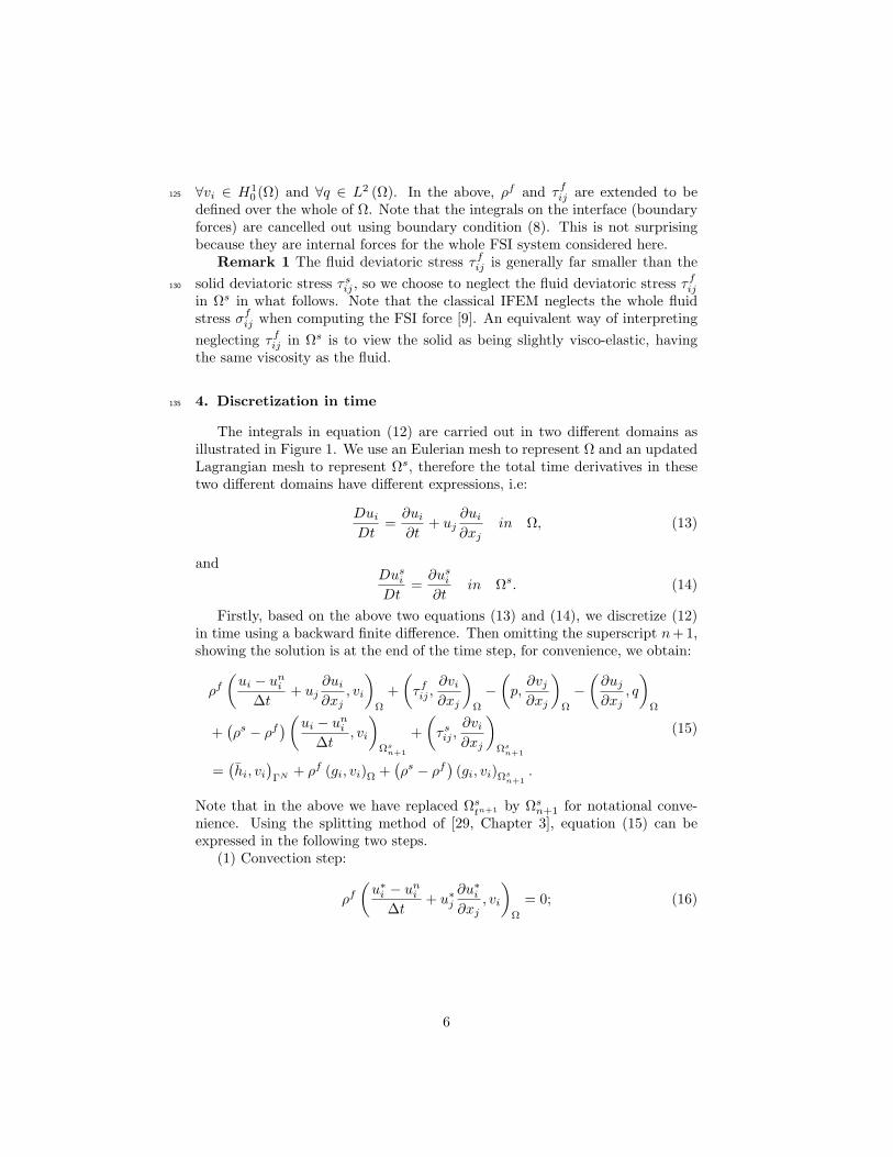
4. Discretization in time135

The integrals in equation (12) are carried out in two different domains asillustrated in Figure 1. We use an Eulerian mesh to represent Ω and an updatedLagrangian mesh to represent Ωs, therefore the total time derivatives in thesetwo different domains have different expressions, i.e:

Dui

Dt=

∂ui

∂t+ uj

∂ui

∂xj

in Ω, (13)

andDus

i

Dt=

∂usi

∂tin Ωs. (14)

Firstly, based on the above two equations (13) and (14), we discretize (12)in time using a backward finite difference. Then omitting the superscript n+1,showing the solution is at the end of the time step, for convenience, we obtain:

ρf(

ui − uni

∆t+ uj

∂ui

∂xj

, vi

)

Ω

+

(

τfij ,∂vi∂xj

)

Ω

−

(

p,∂vj∂xj

)

Ω

−

(

∂uj

∂xj

, q

)

Ω

+(

ρs − ρf)

(

ui − uni

∆t, vi

)

Ωsn+1

+

(

τ sij ,∂vi∂xj

)

Ωsn+1

=(

hi, vi)

ΓN + ρf (gi, vi)Ω +(

ρs − ρf)

(gi, vi)Ωsn+1

.

(15)

Note that in the above we have replaced Ωstn+1 by Ωs

n+1 for notational conve-nience. Using the splitting method of [29, Chapter 3], equation (15) can beexpressed in the following two steps.

(1) Convection step:

ρf(

u∗

i − uni

∆t+ u∗

j

∂u∗

i

∂xj

, vi

)

Ω

= 0; (16)

6

(2) Diffusion step:

ρf(

ui − u∗

i

∆t, vi

)

Ω

+

(

τfij ,∂vi∂xj

)

Ω

−

(

p,∂vj∂xj

)

Ω

−

(

∂uj

∂xj

, q

)

Ω

+(

ρs − ρf)

(

ui − uni

∆t, vi

)

Ωsn+1

+

(

τ sij ,∂vi∂xj

)

Ωsn+1

=(

hi, vi)

ΓN + ρf (gi, vi)Ω +(

ρs − ρf)

(gi, vi)Ωsn+1

.

(17)

The treatment of the above two steps is described separately in the followingsubsections.140

5. Linearization of the convection step

In this section, two methods are introduced to treat the convection equation:Least-squares method and Taylor-Galerkin method, both of which can be used inthe framework of the proposed scheme. Some numerical results for comparisonbetween these two methods are discussed subsequently in section 5. Because145

the overall scheme is explicit, all non-linear terms are linearized using the valuesfrom the last time step. Of course, the scheme can be made implicit with thesame linearized form by iterating within each time step starting from the valueat the last time step.

5.1. Least-squares method150

Linearization of equation (16) gives,

(

u∗

i +∆t

(

u∗

j

∂uni

∂xj

+ unj

∂u∗

i

∂xj

)

, vi

)

Ω

=

(

uni +∆tun

j

∂uni

∂xj

, vi

)

Ω

. (18)

For Least-squares method [30], we may choose the test function in the followingform:

vi = L (wi) = wi +∆t

(

wj

∂uni

∂xj

+ unj

∂wi

∂xj

)

Ω

, (19)

where wi ∈ H10 (Ω). In such a case, the weak form of (16) is:

(L (u∗

i ) , L (wi))Ω =

(

uni +∆tun

j

∂uni

∂xj

, L (wi)

)

Ω

. (20)

In our method a standard biquadratic finite element space is used to discretizeequation (20) directly.

5.2. Taylor-Galerkin method

It is also possible to linearize equation (16) as:

(

u∗

i − uni

∆t+

1

2unj

∂

∂xj

(u∗

i + uni ) , vi

)

Ω

= 0 (21)

7

or(

u∗

i − uni

∆t+ un

j

∂uni

∂xj

, vi

)

Ω

= 0. (22)

Rewriting (22) as

u∗

i = uni −∆tun

j

∂uni

∂xj

, (23)

substituting (23) into equation (21), and applying integration by parts we ob-tain:

(

u∗

i − uni

∆t+ un

j

∂uni

∂xj

, vi

)

Ω

= −∆t

2

(

unk

∂uni

∂xk

, unj

∂vi∂xj

)

Ω

, (24)

where the boundary integral is neglected because uni is the solution of the previ-

ous diffusion step, which means no convection exists on the boundary after thediffusion step. Finally the weak form of Taylor-Galerkin method [29, Chapter2] can be expressed, by rearranging the last equation, as:

(u∗

i , vi)Ω =

(

uni −∆tun

j

∂uni

∂xj

, vi

)

Ω

−∆t2

2

(

unk

∂uni

∂xk

, unj

∂vi∂xj

)

Ω

. (25)

6. Linearization of the diffusion step

As mentioned above, the overall scheme is explicit, so all the derivatives arecomputed on the known coordinate (xs

i )n(denoted xn

i for convenience). Onecould also construct xn+1

i at each time step and take derivatives with respect toxn+1i , however we do not consider such an approach in this article. According

to the definition of τ sij in equation (6),

(

τ sij)n+1

= µs

(

∂xn+1i

∂Xk

∂xn+1j

∂Xk

− δij

)

. (26)

The last equation, using a chain rule, can also be expressed as:

(

τ sij)n+1

= µs

(

∂xn+1i

∂xnk

∂xn+1j

∂xnk

− δij

)

+ µs ∂xn+1i

∂xnk

(

∂xnk

∂Xm

∂xnl

∂Xm

− δkl

)

∂xn+1j

∂xnl

, (27)

and then(

τ sij)n+1

can be expressed by coordinate xni as follows:

(

τ sij)n+1

= µs

(

∂xn+1i

∂xnk

∂xn+1j

∂xnk

− δij

)

+∂xn+1

i

∂xnk

(τ skl)n ∂xn+1

j

∂xnl

. (28)

8

Using xn+1i − xn

i = un+1i ∆t, which is the displacement at the current step, the

last equation may be expressed as:

(

τ sij)n+1

= µs∆t

(

∂un+1i

∂xnj

+∂un+1

j

∂xni

+∆t∂un+1

i

∂xnk

∂un+1j

∂xnk

)

+(

τ sij)n

+∆t2∂un+1

i

∂xnk

(τ skl)n ∂un+1

j

∂xnl

+∆t∂un+1

i

∂xnk

(

τ skj)n

+∆t (τ sil)n ∂un+1

j

∂xnl

.

(29)

Finally, after linearization of the last equation, the weak form (17) can be ex-pressed as:

ρf(

ui − u∗

i

∆t, vi

)

Ω

+(

ρs − ρf)

(

usi − (us

i )n

∆t, vi

)

Ωsn+1

+ µf

(

∂ui

∂xj

+∂uj

∂xi

,∂vi∂xj

)

Ω

−

(

p,∂vj∂xj

)

Ω

−

(

∂uj

∂xj

, q

)

Ω

+ µs∆t

(

∂ui

∂xj

+∂uj

∂xi

+∆t∂ui

∂xk

∂unj

∂xk

+∆t∂un

i

∂xk

∂uj

∂xk

,∂vi∂xj

)

Ωsn+1

+∆t2(

∂ui

∂xk

(τ skl)n ∂un

j

∂xl

+∂un

i

∂xk

(τ skl)n ∂uj

∂xl

,∂vi∂xj

)

Ωsn+1

+∆t

(

∂ui

∂xk

(

τ skj)n

+ (τ sil)n ∂uj

∂xl

,∂vi∂xj

)

Ωsn+1

=(

hi, vi)

ΓN + ρf (gi, vi)Ω +(

ρs − ρf)

(gi, vi)Ωsn+1

+

(

µs∆t2∂un

i

∂xk

∂unj

∂xk

+∆t2∂un

i

∂xk

(τ skl)n ∂un

j

∂xl

−(

τ sij)n

,∂vi∂xj

)

Ωsn+1

.

(30)

The spatial discretization of the above linearized weak form will be discussed155

in the following section, along with the overall solution algorithm.

7. Discretization in space and solution algorithm

7.1. Spatial discretization

We shall use a fixed Eulerian mesh for Ω and an updated Lagrangian meshfor Ωs

n+1 to discretize equation (30). First, we discretize Ω as Ωh using P2P1 el-ements (the Taylor-Hood element) with the corresponding finite element spacesas

V h(Ωh) = span ϕ1, · · · , ϕNu ⊂ H1 (Ω)

andLh(Ωh) = span φ1, · · · , φNp ⊂ L2 (Ω) .

9

The approximated solution uh and ph can be expressed in terms of these basisfunctions as

uh(x) =

Nu

∑

i=1

u(xi)ϕi(x), ph(x) =

Np

∑

i=1

p(xi)φi(x). (31)

We further discretize Ωsn+1 as Ωsh

n+1 (actually it is discretized once on Ωs0

and then updated from the previous mesh) using P1 elements (bilinear triangleelement) with the corresponding finite element spaces as:

V sh(Ωshn+1) = span ϕs

1, · · · , ϕsNs ⊂ H1

(

Ωsn+1

)

,

and approximate uh(x)∣

∣

x∈Ωshn+1

as:

ush (x) =

Ns

∑

i=1

uh(xsi )ϕ

si (x) =

Ns

∑

i=1

Nu

∑

j=1

u(xj)ϕj(xsi )ϕ

si (x), (32)

where xsi is the nodal coordinate of the solid mesh. Notice that the above

approximation defines an L2 projection Pn+1 from V h to V sh: Pn+1

(

uh(x))

=160

ush (x).Substituting (31), (32) and similar expressions for the test functions vh, qh

and vsh into equation (30) gives the following matrix form:

[

A B

BT 0

](

u

p

)

=

(

b

0

)

, (33)

whereA = M/∆t+K+DT (Ms/∆t+Ks)D, (34)

andb = f +DTfs +Mu∗/∆t+DTMsDun/∆t. (35)

In the above, matrix D is the isoparametric interpolation matrix derivedfrom equation (32) which can be expressed as

D =

[

PT 0

0 PT

]

,Pij = ϕi(xsj).

All the other matrices and vectors arise from standard FEM discretization: Mand Ms are mass matrices from discretization of integrals in Ωh (with shapefunction ϕi) and Ωsh (with shape function ϕs

i ) respectively, and similarly for

stiffness matrices K and Ks. B is from discretization of integral −(

p,∂vj

∂vj

)

in165

(30). The force vectors f and fs come from discretization of integrals on theright-hand side of (30) in Ωh and Ωsh respectively. The specific expressions ofthese matrices and vectors can be found in Appendix A.

10

7.2. Overall solution algorithm

Having derived a discrete system of equations we now describe the solution170

algorithm at each time step.

(1) Given the solid configuration (xs)nand velocity field un =

(

uf)n

in Ωf

(us)n

in Ωs

at time step n.

(2) Discretize the convection equation (20) or (25) and solve it to get an inter-mediate velocity u∗.175

(3) Compute the interpolation matrix and solve equation (33) using u∗ and(us)

nas initial values to get velocity field un+1.

(4) Compute solid velocity (us)n+1

= Dun+1 and update the solid mesh by

(xs)n+1

= (xs)n+∆t (us)

n+1, then go to step (1) for the next time step.

Remark 2 The choice of P1 element for an updated domain Ωs is convenient,180

because the form of the bilinear shape functions stays the same when updatingthe nodal coordinates using (xs)

n+1= (xs)

n+∆t (us)

n+1.

Remark 3 When implementing the algorithm, it is unnecessary to performthe matrix multiplication DTKsD globally, because the FEM interpolation islocally based. All the matrix operations can be computed based on the local185

element matrices only. Alternatively, if an iterative solver is used, it is actuallyunnecessary to compute DTKsD. What an iterative step needs is to compute(

DTKsD)

u for a given vector u, therefore one can compute Du first, thenKs (Du), and last DT (KsDu).

8. Numerical experiments190

In this section, we present some numerical examples that have been selectedto allow us to assess the accuracy and the versatility of our proposed numer-ical scheme. We demonstrate convergence in time and space, furthermore, wefavourably compare results with those obtained using monolithic approachesand IFEM, as well as compare against results from laboratory experiment.195

In order to improve the computational efficiency, an adaptive spatial meshwith hanging nodes is used in all the following numerical experiments. Readerscan reference [31, 32, 33, 34] for details of the treatment of hanging nodes. TheLeast-squares method (section 5.1) is used to treat the convection step in alltests unless stated otherwise.200

8.1. Oscillation of a flexible leaflet oriented across the flow direction

This numerical example is used by [15, 16, 17] to validate their methods. Wefirst use the same parameters as used in the above three publications in orderto compare results and test convergence in time and space. We then use a widerange of parameters to show the robustness of our method. The computational205

domain and boundary conditions are illustrated in Figure 2.

11

Figure 2: Computational domain and boundary conditions, taken from [16].

Fluid LeafletL = 4.0 m w = 0.0212 mH = 1.0 m h = 0.8 m

ρf = 100 kg/m3 ρs = 100 kg/m3

µf = 10 N · s/m2 µs = 107 N/m2

Table 1: Properties and domain size for test problem 8.1with a leaflet oriented across the flow direction.

The inlet flow is in the x-direction and given by ux = 15.0y (2− y) sin (2πt).Gravity is not considered in the first test (i.e. g = 0), and other fluid and solidproperties are presented in Table 1.

The leaflet is approximated with 1200 linear triangles with 794 nodes (medium210

mesh size), and the corresponding fluid mesh is adaptive in the vicinity of theleaflet so that it has a similar size. A stable time step ∆t = 5.0 × 10−4s isused in these initial simulations. The configuration of the leaflet is illustratedat different times in Figure 3.

Previously published numerical results are qualitatively similar to those in215

Figure 3 but show some quantitative variations. For example, [16] solved afully-coupled system but the coupling is limited to a line, and the solid in theirresults (Figure 7 (l)) behaves as if it is slightly harder. Alternatively, [15] useda fractional step scheme to solve the FSI equations combined with a penaltymethod to enforce the incompressibility condition. In their results (Fig. 3 (h))220

the leaflet behaves as if it is slightly softer than [16] and harder than [17]. In [17]a beam formulation is used to describe the solid. The fluid mesh is locally refinedusing hierarchical B-Splines, and the FSI equation is solved monolithically. Theleaflet in their results (Fig. 34) behaves as softer than the other two consideredhere. Our results in Figure 3 are most similar to those of [17]. This may be225

seen more precisely by inspection of the graphs of the oscillatory motion of theleaflet tip in Figure 4, corresponding to Fig. 32 in [17]. We point out herethat Taylor-Galerkin method has also been used to solve the convection stepfor this test, and we gain almost the same accuracy using the same time step∆t = 5.0 × 10−4s. Having validated our results for this example against the230

12

(a) t = 0.1s

(b) t = 0.2s

(c) t = 0.6s

(d) t = 0.8s

Figure 3: Configuration of leaflet and magnitude of velocity on the adaptive fluid mesh.

work of others, we shall use this test case to further explore more details of ourmethod.

We commence by testing the influence of the ratio of fluid and solid meshsizes rm=(local fluid element area)/(solid element area). Fixing the fluid meshsize, three different solid mesh sizes are chosen: coarse (640 linear triangles with235

403 nodes rm ≈ 1.5), medium (1200 linear triangles with 794 nodes rm ≈ 3.0)and fine (2560 linear triangles with 1445 nodes rm ≈ 5.0), and a stable timestep ∆t = 5.0×10−4s is used. From these tests we observe that there is a slight

13

Figure 4: Evolution of horizontal and vertical displacement at top right corner of the leaflet.

difference in the solid configuration for different meshes, as illustrated at t = 0.6sin Figure 5. Significantly however, the difference in displacement decreases as240

the solid mesh becomes finer. Further, we found that 1.5 ≤ rm ≤ 5.0 ensuresthe stability of the proposed approach. Note that we use a 9-node quadrilateralfor the fluid velocity and 3-node triangle for solid velocity, so rm ≈ 3.0 meansthe fluid and solid mesh locally have a similar number of nodes for velocity.

(a)coarse (b)medium (c)fine

Figure 5: Configuration of leaflet for different mesh ratio rm,and contour plots of displacement magnitude at t = 0.6s.

We next consider convergence tests undertaken for refinement of both the245

fluid and solid meshes with the fixed ratio of mesh sizes rm ≈ 3.0. Four differentlevels of meshes are used, the solid meshes are: coarse (584 linear triangleswith 386 nodes), medium (1200 linear triangles with 794 nodes), fine (2560linear triangles with 1445 nodes), and very fine (3780 linear triangles with 2085nodes). The fluid meshes have the corresponding sizes with the solid at their250

maximum refinement level. As can be seen in Figure 6 and Table 2, the velocityis converging as the mesh becomes finer.

In addition, we consider tests of convergence in time using a fixed ratio offluid and solid mesh sizes rm ≈ 3.0. Using the medium solid mesh size and thesame fluid mesh size as above, results are shown in Figure 7 and Table 3. From255

these it can be seen that the velocities are converging as the time step decreases.

14

(a) Coarse (b) Medium

(c) Fine (d) Very fine

Figure 6: Contour plots of horizontal velocity at t = 0.5s.

Between different mesh sizesDifference of maximum

horizontal velocity at t = 0.5scoarse and medium 0.01497medium and fine 0.00214fine and very fine 0.00190

Table 2: Comparison of maximum velocity for different meshes.

(a) ∆t = 2.0 × 10−3s(breaks down at t = 0.61s).

(b) ∆t = 1.0 × 10−3s.

(c) ∆t = 5.0 × 10−4s. (d) ∆t = 2.5 × 10−4s.

Figure 7: Contour plots of horizontal velocity at t = 0.5s.

15

Steps sizes comparedDifference of maximum

horizontal velocity at t = 0.5s∆t = 2.0× 10−3 and ∆t = 1.0× 10−3 0.00854∆t = 1.0× 10−3 and ∆t = 5.0× 10−4 0.00517∆t = 5.0× 10−4 and ∆t = 2.5× 10−4 0.00263

Table 3: Comparison of maximum velocity for different time step size.

(a) ρr = 1, Re = 100 and Fr = 0. (b) ρr = 1, µs = 103 and Fr = 0.

(c) Re = 100, µs = 103 and Fr = 0. (d) Re = 100 and µs = 103.

Figure 8: Parameters sets and results, ∆t = 5.0 × 10−4s for Group (b)∼(d).

Finally, in order to assess the robustness of our approach, we vary each ofthe physical parameters using three different cases as shown in Figure 8. Amedium mesh size with fixed rm ≈ 3.0 is used to undertake all of these tests.The dimensionless parameters shown in Figure 8 are defined as: ρr = ρs

ρf , µs =260

µs

ρfU2 , Re = ρfUHµf and Fr = gH

U2 where the average velocity U = 10 in thisexample. The period of inlet flow is T = 1.

It can be seen from the results of group (a) that the larger the value of shearmodulus µs the harder the solid behaves, however a smaller time step is required.For the case of µs = 109, the solid behaves almost like a rigid body, as we would265

expect. From the results of group (b) it is clear that the Reynolds Number (Re)has a large influence on the behaviour of the solid. The density and gravity haverelatively less influence on the behaviour of solid in this problem which can beseen from the results of group (c) and group (d) respectively.

16

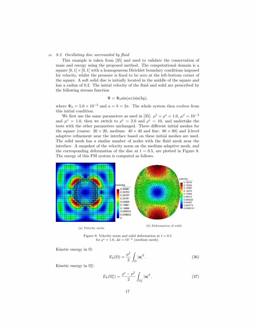
8.2. Oscillating disc surrounded by fluid270

This example is taken from [35] and used to validate the conservation ofmass and energy using the proposed method. The computational domain is asquare [0, 1]× [0, 1] with a homogeneous Dirichlet boundary conditions imposedfor velocity, whilst the pressure is fixed to be zero at the left-bottom corner ofthe square. A soft solid disc is initially located in the middle of the square andhas a radius of 0.2. The initial velocity of the fluid and solid are prescribed bythe following stream function

Ψ = Ψ0sin(ax)sin(by),

where Ψ0 = 5.0 × 10−2 and a = b = 2π. The whole system then evolves fromthis initial condition.

We first use the same parameters as used in [35]: ρf = ρs = 1.0, µf = 10−3

and µs = 1.0, then we switch to ρs = 2.0 and ρs = 10, and undertake thetests with the other parameters unchanged. Three different initial meshes forthe square (coarse: 20 × 20, medium: 40 × 40 and fine: 80 × 80) and 2-leveladaptive refinement near the interface based on these initial meshes are used.The solid mesh has a similar number of nodes with the fluid mesh near theinterface. A snapshot of the velocity norm on the medium adaptive mesh, andthe corresponding deformation of the disc at t = 0.5, are plotted in Figure 9.The energy of this FSI system is computed as follows.

(a) Velocity norm.(b) Deformation of solid.

Figure 9: Velocity norm and solid deformation at t = 0.5for ρs = 1.0, ∆t = 10−3 (medium mesh).

Kinetic energy in Ω:

Ek(Ω) =ρf

2

∫

Ω

|u|2. (36)

Kinetic energy in Ωst :

Ek(Ωst ) =

ρs − ρf

2

∫

Ωst

|u|2. (37)

17

Viscous dissipation in Ω:

Ed(Ω) =

∫ t

0

∫

Ω

τfij∂ui

∂xj

. (38)

Potential energy of solid:

Ep(Ωs0) =

µs

2

∫

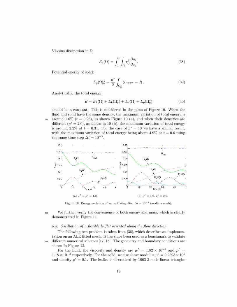
Ωs0

(trFFT − d) . (39)

Analytically, the total energy

E = Ek(Ω) + Ek(Ωst ) + Ed(Ω) + Ep(Ω

s0) (40)

should be a constant. This is considered in the plots of Figure 10. When thefluid and solid have the same density, the maximum variation of total energy isaround 1.6% (t = 0.26), as shown Figure 10 (a), and when their densities are275

different (ρs = 2.0), as shown in 10 (b), the maximum variation of total energyis around 2.2% at t = 0.31. For the case of ρs = 10 we have a similar result,with the maximum variation of total energy being about 4.9% at t = 0.6 usingthe same time step ∆t = 10−3.

(a) ρf = ρs = 1.0. (b) ρf = 1.0, ρs = 2.0.

Figure 10: Energy evolution of an oscillating disc, ∆t = 10−3 (medium mesh).

We further verify the convergence of both energy and mass, which is clearly280

demonstrated in Figure 11.

8.3. Oscillation of a flexible leaflet oriented along the flow direction

The following test problem is taken from [36], which describes an implemen-tation on an ALE fitted mesh. It has since been used as a benchmark to validatedifferent numerical schemes [17, 18]. The geometry and boundary conditions are285

shown in Figure 12.For the fluid, the viscosity and density are µf = 1.82 × 10−4 and ρf =

1.18× 10−3 respectively. For the solid, we use shear modulus µs = 9.2593× 105

and density ρs = 0.1. The leaflet is discretized by 1063 3-node linear triangles

18

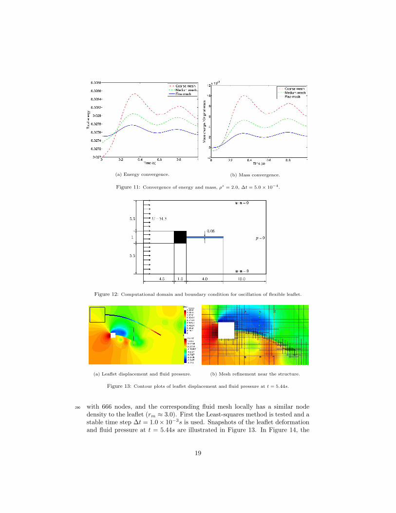
(a) Energy convergence. (b) Mass convergence.

Figure 11: Convergence of energy and mass, ρs = 2.0, ∆t = 5.0 × 10−4.

Figure 12: Computational domain and boundary condition for oscillation of flexible leaflet.

(a) Leaflet displacement and fluid pressure. (b) Mesh refinement near the structure.

Figure 13: Contour plots of leaflet displacement and fluid pressure at t = 5.44s.

with 666 nodes, and the corresponding fluid mesh locally has a similar node290

density to the leaflet (rm ≈ 3.0). First the Least-squares method is tested and astable time step ∆t = 1.0× 10−3s is used. Snapshots of the leaflet deformationand fluid pressure at t = 5.44s are illustrated in Figure 13. In Figure 14, the

19

Figure 14: Distribution of pressure across the leaflet on the three lines in Figure 13 (b).

distributions of pressure across the leaflet corresponding to the three lines (AB,CD and EF) in Figure 13 (b) are plotted, from which we can observe that the295

sharp jumps of pressure across the leaflet are captured.The evolution of the vertical displacement of the leaflet tip with respect to

time is plotted in Figure 15(a). Both the magnitude (1.34) and the frequency(2.94) have a good agreement with the result of [36], using a fitted ALE meshand of [17], using a monolithic unfitted mesh approach. Taylor-Galerkin method300

is also tested using ∆t = 2.0× 10−4s as a stable time step, and a correspondingresult is shown in 15(b). This shows a similar magnitude (1.24) and frequency(2.86). These results are all within the range of values in [17, Table 4]. Notethat since the initial condition before oscillation for these simulations is anunstable equilibrium, the first perturbation from this regime is due to numerical305

disturbances. Consequently, the initial transient regimes observed for the twomethods (Least-squares and Taylor-Galerkin methods) are quite different. Itis possible that an explicit method causes these numerical perturbations moreeasily, therefore makes the leaflet start to oscillate at an earlier stage than whenusing Least-squares approach.310

(a) Least-squares method. (b) Taylor-Galerkin method.

Figure 15: Displacement of leaflet tip as a function of time.

20

8.4. Solid disc in a cavity flow

This numerical example is used to compare our method with the IFEM,which is described in [11, 35]. In order to compare in detail, we also implementthe IFEM, but we implemented it on an adaptive mesh with hanging nodes, andwe use the isoparametric FEM interpolation function rather than the discretized315

delta function or RKPM function of [9, 10].The fluid and solid properties are chosen to be the same as in [35]: ρf =

ρs = 1.0, µf = 0.01 and µs = 0.1. The horizontal velocity on the top boundaryof the cavity is prescribed as 1 and the vertical velocity is fixed to be 0 as shownin Figure 16. The velocities on the other three boundaries are all fixed to be 0,320

and pressure at the bottom-left point is fixed to be 0 as a reference point.

Figure 16: Computational domain forcavity flow, taken from [35].

Figure 17: Adaptive mesh forcavity flow.

In order to compare our method with IFEM we use the same meshes for fluidand solid: the solid mesh has 2381 nodes and the fluid mesh locally has a similarnumber of nodes (adaptive, see Figure 17). First the Least-squares method isused to solve the convection step, and the time step is ∆t = 1.0× 10−3. Figure325

18 shows the configuration of the deformed disc at different stages, from whichwe do not observe significant differences of the velocity norm even for a longrun as shown in Figure 18 (b). Then Taylor-Galerkin method is tested, and weachieve almost the same accuracy by using the same time step (not shown inthe Figure).330

We also test different densities, and the cases of µs = 1.0 and µs = 100. Forour proposed method we can use µs = 100 or larger in order to make the solidbehave like a rigid body without changing time step (again, not shown here dueto lack of space). This is not possible for the IFEM for which the simulationalways breaks down for µs = 100, however small the time step, due to the huge335

FSI force on the right-hand side of the IFEM system.

8.5. Falling disc in a channel with gravity

The final test that we present in this paper is that of a falling disc in achannel, as cited by [10, 18] for example, in order to further validate against the

21

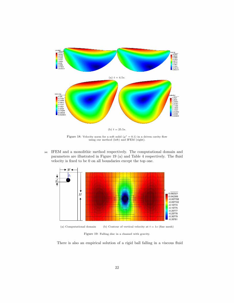
(a) t = 4.5s.

(b) t = 25.5s.

Figure 18: Velocity norm for a soft solid (µs = 0.1) in a driven cavity flowusing our method (left) and IFEM (right).

IFEM and a monolithic method respectively. The computational domain and340

parameters are illustrated in Figure 19 (a) and Table 4 respectively. The fluidvelocity is fixed to be 0 on all boundaries except the top one.

(a) Computational domain (b) Contour of vertical velocity at t = 1s (fine mesh)

Figure 19: Falling disc in a channel with gravity.

There is also an empirical solution of a rigid ball falling in a viscous fluid

22

Fluid DiscW = 2.0 cm d = 0.125 cmH = 4.0 cm h = 0.5 cm

ρf = 1.0 g/ cm3 ρs = 1.2 g/ cm3

µf = 1.0 dyne · s/ cm2 µs = 108 dyne/ cm2

g = 980 cm/ s2 g = 980 cm/ s2

Table 4: Fluid and material properties of a falling disc.

[18], for which the terminal velocity, ut, under gravity is given by

ut =

(

ρs − ρf)

gr2

4µf

(

ln

(

L

r

)

− 0.9157 + 1.7244( r

L

)2

− 1.7302( r

L

)4)

, (41)

where ρs and ρf are the density of solid and fluid respectively, µf is viscosityof the fluid, g = 980 cm/ s2 is acceleration due to gravity, L = W/ 2 and r isthe radius of the falling ball. We choose µs = 108 dyne/ cm2 to simulate a345

rigid body here, and µs = 1012 dyne/ cm2 is also applied, which gives virtuallyidentical results.

Three different meshes are used: the disc boundary is represented with 28nodes (coarse), 48 nodes (medium), or 80 nodes (fine). The fluid mesh near thesolid boundary has the same mesh size as that of the disc, and a stable time step350

t = 0.005s is used for all three cases. A local snapshot of the vertical velocitywith the adaptive mesh is shown in Figure 19 (b). From the fluid velocitypattern around the disc we can observe that the disc behaves like a rigid bodyas expected. In addition, the evolution of the velocity of the mid-point of thedisc is shown in Figure 20, from which it can be seen that the numerical solution355

converges from below to the empirical solution.

Figure 20: Evolution of velocity at the center of a falling disc.(The blue solid line represents the empirical solution from formula (41),

for interpretation of the reference to color, the reader is referred to the web version.)

23

9. Discussion

In this section, some further remarks and notes concerning the proposedmethod are discussed.

9.1. Treatment of the convection equation360

Both the Least-squares method and Taylor-Galerkin method add artificialdiffusive terms in their formulations to stabilize the numerical scheme. Like allsuch stabilisation approaches this necessarily has an influence on the accuracy,especially for large Reynolds numbers. In such cases a balance is required be-tween minimizing the artificial dissipation and maintaining a stable time step365

size that is acceptable. In our applications, the Reynolds number is around100 ∼ 500, except for two extreme test cases in section 8.1 whose Reynoldsnumbers are 1000 and 5000 respectively (Figure 8 (b)). Even then, in thesecases a minimal amount of diffusion is observed provided we use a small timestep (5 × 10−4). Alternatively, an upwind scheme or a discontinuous Galerkin370

method could be a better choice. However, we have not yet implemented suchmethods on the adaptive mesh with hanging nodes.

9.2. The Lagrangian update of the solid

Updating the solid based upon its velocity could lead to distorted elements,either in its interior or at its boundary. Should this occur there are advanced375

mesh update techniques to improve the quality of solid mesh [37] or discreteremeshing may be used [7]. However all of the tests undertaken in this articlehave been performed based upon published benchmarks using incompressiblesolids and a small time step, and we have not encountered the problem ofsignificantly distorted elements. In other applications our simple Lagrangian380

approach may not be adequate and so ALE techniques, possibly including meshquality improvement, may also be required.

9.3. Contact between solids and boundaries

In many applications moving solids may run into boundaries (either externalor of other moving bodies). In this article, we have only considered standard385

benchmark problems for which contact does not arise. Hence, through the use ofa small time step and an adaptive algorithm to refine the mesh when the solidsare near each other or near the boundaries, we have not needed to implement acontact test or a contact model. In the future, we do intend to consider addinga contact model in order to further generalize our method.390

9.4. Conditioning of the linear system

If ρs ≥ ρf , and neglecting τfij , the discretized linear equation system isguaranteed to be well-conditioned. However, this restriction is too stringentto be a necessary condition. For example, we have implemented and tested anumber of cases for which ρs < ρf and the solid rises in a stable manner due to395

buoyancy.

24

9.5. Approximation for pressure

It is well known that the pressure jumps across the interface between the fluidand solid, and that a high resolution is therefore needed near the interface inorder to capture this jump. In this article, we use an adaptive mesh refinement400

near the interface to reduce the error caused by our continuous approximation(P2P1 element) for this discontinuous pressure. An alternative or additionalchoice is to use P2 (P1 +C) elements (the shape function of pressure is enrichedby a constant) in order to capture an element-based jump of pressure. We intendto test this element in the future.405

10. Conclusion

In this article we introduce a one-field FD method for fluid-structure interac-tion, which can be applied to a wide range of problems, from small deformationto very large deformation and from very soft solids through to very rigid solids.Several numerical examples, which are widely used in the literature of IFEM and410

FD methods with DLM (DLM/FD), are implemented to validate the proposedmethod.

The one-field FDmethod combines features from both the IFEM and DLM/FD.Nevertheless, it differs from each of them in the following aspects. Firstly, ourone-field FD method solves the solid and fluid equations together while the clas-415

sical IFEM does not solve the solid equations. Although the implicit form ofIFEM can iteratively solve the solid equations, this is different from our one-field FD method which couples the fluid and solid equations monolithically viaa direct matrix addition as shown in formulas (34) and (35). Secondly, whileboth our one-field FD method and DLM/FD solve solid equations, the former420

solves for just one velocity field in the solid domain using FEM interpolation,while the latter solves one velocity field and one displacement field in the soliddomain using Lagrange multipliers. In summary therefore we believe that theone-field FD method has the potential to offer the robustness and range of oper-ation of DLM/FD, but at a computational cost that is much closer to that of the425

IFEM approaches. Expressed another way, we contend that our approach hasall of the advantages of IFEM techniques but the additional robustness usuallyassociated with more complex monolithic solvers.

Appendix A. Expressions of M, Ms, K, Ks, B, f and fs

In this appendix, the specific expressions for the mass matrices M and Ms,430

stiffness matricesK andKs, matrixB and the force vectors f and fs in equations(33), (34) and (35) are presented.

(1) M: (k,m = 1, 2, · · ·Nu)

M = ρf[

M11

M22

]

, (M11)km = (M22)km = (ϕk, ϕm)Ωh .

25

(2) Ms: (k,m = 1, 2, · · ·Ns)

Ms =(

ρs − ρf)

[

Ms11

Ms22

]

, (Ms11)km = (Ms

22)km = (ϕsk, ϕ

sm)Ωsh .

(3) K: (k,m = 1, 2, · · ·Nu)

K = µf

[

K11 K12

K21 K22

]

,

where

(K11)km = 2

(

∂ϕk

∂x1,∂ϕm

∂x1

)

Ωh

+

(

∂ϕk

∂x2,∂ϕm

∂x2

)

Ωh

,

(K22)km = 2

(

∂ϕk

∂x2,∂ϕm

∂x2

)

Ωh

+

(

∂ϕk

∂x1,∂ϕm

∂x1

)

Ωh

,

(K12)km =

(

∂ϕk

∂x1,∂ϕm

∂x2

)

Ωh

, (K21)km = (K12)mk =

(

∂ϕk

∂x2,∂ϕm

∂x1

)

Ωh

.

(4) Ks: (b,m = 1, 2, · · ·Ns)

Ks =

[

Ks11 Ks

12

Ks21 Ks

22

]

,

where

(Ks11)bm = µs∆t2

(

∂ϕsb

∂x1,∂ϕs

m

∂x1

)

Ωsh

+ µs∆t

(

∂ϕsb

∂x2,∂ϕs

m

∂x2

)

Ωsh

+ 2µs∆t2(

∂ϕsb

∂xk

∂un1

∂xk

,∂ϕs

m

∂x1

)

Ωsh

+ µs∆t2(

∂ϕsb

∂xk

∂un2

∂xk

,∂ϕs

m

∂x2

)

Ωsh

+ 2∆t2(

∂ϕsb

∂xk

(τ skl)n ∂un

1

∂xl

,∂ϕs

m

∂x1

)

Ωsh

+∆t2(

∂ϕsb

∂xk

(τ skl)n ∂un

2

∂xl

,∂ϕs

m

∂x2

)

Ωsh

+ 2∆t

(

∂ϕsb

∂xk

(τ sk1)n,∂ϕs

m

∂x1

)

Ωsh

+∆t

(

∂ϕsb

∂xk

(τ sk2)n,∂ϕs

m

∂x2

)

Ωsh

.

Ks22 can be expressed by changing the subscript 1 to 2 and 2 to 1 in the

formula of Ks11.

(Ks12)bm = µs∆t

(

∂ϕsb

∂x1,∂ϕs

m

∂x2

)

Ωsh

+ µs∆t2(

∂un1

∂xk

∂ϕsb

∂xk

,∂ϕs

m

∂x2

)

Ωsh

+∆t2(

∂un1

∂xk

(τ skl)n ∂ϕs

b

∂xl

,∂ϕs

m

∂x2

)

Ωsh

+∆t

(

(τ s1k)n ∂ϕs

b

∂xk

,∂ϕs

m

∂x2

)

Ωsh

,

and (Ks21)bm = (Ks

12)mb.

(5) B: (k = 1, 2, · · ·Np and m = 1, 2, · · ·Nu)

B =

[

B1

B2

]

, (Bi)mk = −

(

φk,∂ϕm

∂xi

)

Ωh

, (i = 1, 2).

26

(6) f : (m = 1, 2, · · ·Nu)

f =

(

f1f2

)

, (fi)m = ρf (gi, ϕm)Ωh +(

hi, ϕm

)

ΓNh , (i = 1, 2)

(7) fs: (m = 1, 2, · · ·Ns)

fs =

(

fs1fs2

)

, (fsi )m =(

ρs − ρf)

(gi, ϕsm)Ωsh

+

(

µs∆t2∂un

i

∂xk

∂unj

∂xk

+∆t2∂un

i

∂xk

(τ skl)n ∂un

j

∂xl

−(

τ sij)n

,∂ϕs

m

∂xj

)

Ωsh

, (i = 1, 2).

References

[1] G. Hou, J. Wang, A. Layton, Numerical methods for fluid-structure in-435

teractiona review, Commun. Comput. Phys 12 (2) (2012) 337–377. doi:

10.4208/cicp.291210.290411s.

[2] U. Kuttler, W. A. Wall, Fixed-point fluid–structure interaction solvers withdynamic relaxation, Computational Mechanics 43 (1) (2008) 61–72. doi:

10.1007/s00466-008-0255-5.440

[3] J. Degroote, K.-J. Bathe, J. Vierendeels, Performance of a new parti-tioned procedure versus a monolithic procedure in fluid–structure inter-action, Computers & Structures 87 (11-12) (2009) 793–801. doi:10.1016/j.compstruc.2008.11.013.

[4] M. Heil, An efficient solver for the fully coupled solution of large-445

displacement fluid–structure interaction problems, Computer Methods inApplied Mechanics and Engineering 193 (1-2) (2004) 1–23. doi:10.1016/j.cma.2003.09.006.

[5] M. Heil, A. L. Hazel, J. Boyle, Solvers for large-displacement fluid–structureinteraction problems: segregated versus monolithic approaches, Computa-450

tional Mechanics 43 (1) (2008) 91–101. doi:10.1007/s00466-008-0270-6.

[6] R. L. Muddle, M. Mihajlovic, M. Heil, An efficient preconditioner formonolithically-coupled large-displacement fluid–structure interaction prob-lems with pseudo-solid mesh updates, Journal of Computational Physics231 (21) (2012) 7315–7334. doi:10.1016/j.jcp.2012.07.001.455

[7] R. C. Peterson, P. K. Jimack, M. A. Kelmanson, The solution oftwo-dimensional free-surface problems using automatic mesh genera-tion, International journal for numerical methods in fluids 31 (6)(1999) 937–960. doi:10.1002/(SICI)1097-0363(19991130)31:6<937::

AID-FLD906>3.0.CO;2-p.460

27

[8] M. A. Walkley, P. H. Gaskell, P. K. Jimack, M. A. Kelmanson, J. L.Summers, Finite element simulation of three-dimensional free-surfaceflow problems, J Sci Comput 24 (2) (2005) 147–162. doi:10.1007/

s10915-004-4611-0.

[9] L. Zhang, A. Gerstenberger, X. Wang, W. K. Liu, Immersed finite ele-465

ment method, Computer Methods in Applied Mechanics and Engineering193 (21) (2004) 2051–2067. doi:doi:10.1016/j.cma.2003.12.044.

[10] L. Zhang, M. Gay, Immersed finite element method for fluid-structureinteractions, Journal of Fluids and Structures 23 (6) (2007) 839–857.doi:10.1016/j.jfluidstructs.2007.01.001.470

[11] X. Wang, L. T. Zhang, Interpolation functions in the immersed boundaryand finite element methods, Computational Mechanics 45 (4) (2009) 321–334. doi:10.1007/s00466-009-0449-5.

[12] X. Wang, C. Wang, L. T. Zhang, Semi-implicit formulation of the immersedfinite element method, Computational Mechanics 49 (4) (2011) 421–430.475

doi:10.1007/s00466-011-0652-z.

[13] X. Wang, L. T. Zhang, Modified immersed finite element method for fully-coupled fluid–structure interactions, Computer Methods in Applied Me-chanics and Engineering 267 (2013) 150–169. doi:10.1016/j.cma.2013.

07.019.480

[14] R. Glowinski, T. Pan, T. Hesla, D. Joseph, J. Periaux, A fictitious domainapproach to the direct numerical simulation of incompressible viscous flowpast moving rigid bodies: Application to particulate flow, Journal of Com-putational Physics 169 (2) (2001) 363–426. doi:10.1006/jcph.2000.6542.

[15] Z. Yu, A DLM/FD method for fluid/flexible-body interactions, Journal of485

Computational Physics 207 (1) (2005) 1–27. doi:10.1016/j.jcp.2004.

12.026.

[16] F. P. Baaijens, A fictitious domain/mortar element method for fluid-structure interaction, International Journal for Numerical Methods inFluids 35 (7) (2001) 743–761. doi:10.1002/1097-0363(20010415)35:490

7<743::AID-FLD109>3.0.CO;2-A.

[17] C. Kadapa, W. Dettmer, D. Peric, A fictitious domain/distributed lagrangemultiplier based fluid–structure interaction scheme with hierarchical b-spline grids, Computer Methods in Applied Mechanics and Engineering301 (2016) 1–27. doi:10.1016/j.cma.2015.12.023.495

[18] C. Hesch, A. Gil, A. A. Carreno, J. Bonet, P. Betsch, A mortar approach forfluid–structure interaction problems: Immersed strategies for deformableand rigid bodies, Computer Methods in Applied Mechanics and Engineering278 (2014) 853–882. doi:10.1016/j.cma.2014.06.004.

28

[19] C. S. Peskin, The immersed boundary method, Acta numerica 11 (2002)500

479–517. doi:10.1016/j.cma.2015.12.023.

[20] A. Robinson-Mosher, C. Schroeder, R. Fedkiw, A symmetric positive defi-nite formulation for monolithic fluid structure interaction, Journal of Com-putational Physics 230 (4) (2011) 1547–1566. doi:10.1016/j.jcp.2010.

11.021.505

[21] E. Hachem, S. Feghali, R. Codina, T. Coupez, Anisotropic adaptive mesh-ing and monolithic variational multiscale method for fluid–structure in-teraction, Computers & Structures 122 (2013) 88–100. doi:10.1016/j.

compstruc.2012.12.004.

[22] O. Pironneau, An energy preserving monolithic Eulerian fluid-structure510

numerical scheme, arXiv:1607.08083v1 [cs.CE] 27 Jul 2016.

[23] F. Auricchio, D. Boffi, L. Gastaldi, A. Lefieux, A. Reali, A study on unfitted1d finite element methods, Computers & Mathematics with Applications68 (12) (2014) 2080–2102. doi:10.1016/j.camwa.2014.08.018.

[24] A. Gerstenberger, W. A. Wall, An extended finite element515

method/Lagrange multiplier based approach for fluid-structure inter-action, Computer Methods in Applied Mechanics and Engineering197 (19-20) (2008) 1699–1714. doi:10.1016/j.cma.2007.07.002.

[25] S. Frei, Eulerian finite element methods for interface problems and fluid-structure interactions, Ph.D. thesis, Universitt Heidelberg (2016).520

[26] T. Richter, A fully Eulerian formulation for fluid–structure-interactionproblems, Journal of Computational Physics 233 (2013) 227–240. doi:

10.1016/j.jcp.2012.08.047.

[27] T. Wick, Coupling of fully Eulerian and arbitrary Lagrangian–Eulerianmethods for fluid-structure interaction computations, Computational Me-525

chanics 52 (5) (2013) 1113–1124. doi:10.1007/s00466-013-0866-3.

[28] T. Dunne, R. Rannacher, Adaptive finite element approximation of fluid-structure interaction based on an Eulerian variational formulation, in: Lec-ture Notes in Computational Science and Engineering, Springer ScienceBusiness Media, 2006, pp. 110–145. doi:10.1007/3-540-34596-5_6.530

[29] O. Zienkiewic, The finite element method for fluid dynamics, 6th Edition,Elsevier BV, 2005.

[30] P. B. Bochev, M. D. Gunzburger, Least-squares finite element methods,Vol. 166, Springer Science & Business Media, 2009.

[31] A. K. Gupta, A finite element for transition from a fine to a coarse grid,535

International Journal for Numerical Methods in Engineering 12 (1) (1978)35–45. doi:10.1002/nme.1620120104.

29

[32] T.-P. Fries, A. Byfut, A. Alizada, K. W. Cheng, A. Schrder, Hanging nodesand XFEM, International Journal for Numerical Methods in Engineering86 (4-5) (2010) 404–430. doi:10.1002/nme.3024.540

[33] W. Bangerth, O. Kayser-Herold, Data structures and requirements for hp fi-nite element software, ACM Transactions on Mathematical Software 36 (1)(2009) 1–31. doi:10.1145/1486525.1486529.

[34] N. Zander, T. Bog, S. Kollmannsberger, D. Schillinger, E. Rank, Multi-level hp-adaptivity: high-order mesh adaptivity without the difficulties of545

constraining hanging nodes, Computational Mechanics 55 (3) (2015) 499–517. doi:10.1007/s00466-014-1118-x.

[35] H. Zhao, J. B. Freund, R. D. Moser, A fixed-mesh method for incom-pressible flow–structure systems with finite solid deformations, Journal ofComputational Physics 227 (6) (2008) 3114–3140. doi:10.1016/j.jcp.550

2007.11.019.

[36] W. A. Wall, Fluid-struktur-interaktion mit stabilisierten finiten elementen,Ph.D. thesis, Universitt Stuttgart (1999). doi:10.18419/OPUS-127.

[37] Y. Bazilevs, K. Takizawa, T. E. Tezduyar, Computational Fluid-StructureInteraction: Methods and Applications, Wiley-Blackwell, 2013. doi:10.555

1002/9781118483565.

30