Embed Size (px)
Citation preview


A numerical study of the effect of aortic wall
compliance and blood flow through the ascending
aorta
Helen Lorna Morrissey
Thesis presented in fulfillment
blah blah blah for the Degree of BSc in Mechanical Engineering
Department of Mechanical Engineering
University of Cape Town
November 1, 2006

Abstract
The ascending aorta is located at the outflow tract of the heart and its function is to
supply the body with oxygenated blood from the lungs. Any damage to the ascending
aorta as a result of age or disease can have severe effects on the entire body.
A computational study of both the artery wall tissue and the blood flow in the aorta and
the coupling of these two systems, to find the effects on aortic compliance is described
in this report. The investigation involved one fluid model (analysed with CFD) coupled
with three models of a healthy aorta, and one model of a diseased aorta (analysed with
FEM). Various programmes were created in Matlab to couple the solid and fluid systems.
The aorta was modelled as a straight cylinder and thus the solid and fluid models were
assumed as axi-symmetric. Blood was modelled as Newtonian, with constant density
and viscosity values. A steady blood flow model was defined, and the flow was modelled
as laminar.
Arteries are comprised of three layers, the intima, media and adventitia, however the
intimal layer is very thin in a healthy artery and its effect was assumed negligible
in the healthy artery models. Constitutive equations were developed for the artery
walls, which described a linear elastic, transversely isotropic material. A bottom-up
engineering approach was taken and the aorta was first modelled as isotropic, consisting
of only one averaged layer, then as isotropic, consisting of an adventitial layer and a
medial layer, and finally as orthotropic, consisting of the adventitial and medial layers.
The thickening of the intima was then induced in the models to approximate an artery
affected by arteriosclerosis.
The results showed an increase in aortic compliance from the initial model to the
final model. It was also found that the effect of blood flow in the coupled simulations
increased the compliance of the ascending aorta.
It was concluded that as the values of compliance were within the measured range
under physiological conditions the coupled investigation was successful. However various
improvements can be made to the models, in terms of the material models, pulsatility
of the blood flow and a three-dimensional model of the aorta.

Declaration
1 I know that plagiarism is wrong. Plagiarism is to use of another’s work and pretend
that it is one’s own.
2 I have used the Vancouver convention for citation and referencing. Each significant
contribution to, and quotation in, this report from the works of other
people has been attributed, and has been cited and referenced.
3 This report is my own work.
4 I have not allowed, and will not allow anyone to copy my work with the intention of
passing it off as his or her own work.
Signature ........................................................
Helen Lorna Morrissey
i

Acknowledgements
I would like to thank Dr C.J. Meyer for his help and concern during the course of this
project; in spite of his broken leg he has done everything he can to make his students as
comfortable as possible with their theses. Thank you to Professor B.D. Reddy for his
calm and reassuring assistance in this project and for knowing everything that I don’t.
I would also like to thank him and Dr T. Franz for proposing such an interesting topic
and allowing me to tackle it.
Thanks must also go to Helena vd Merwe for her willingness to help me with any
ABAQUS R© problems that I encountered, and for making her way up to Upper Campus
just for this purpose.
I would like to thank everyone at BISRU for being so willing to help me with
ABAQUS R© , especially to Pierre le Roux for his general support and Victor Balden
for solving my three week problems in the space of two hours.
The help received from the post-graduates in CERECAM has been indispensable in
this project, thank heavens for you guys. Thank you for teaching me almost everything
I know about computers; no more editing documents with black fineliner. So thank you
Andrew, Amy, Darnell, Dwain, JP, Kevin and Vani, you may have saved my life a few
times.
My undergraduate colleagues, thanks so much, you have been both entertaining and
supportive. A special thank you goes to Marlan Perumal, what would I have done with-
out you?
Finally, thank you to my family, friends and Beetchis, for their endless encouragement
and support, you are my gifts from God.
ii

Nomenclature
Symbols
Cd Compliance
Dd Diameter (m)
E Elastic modulus (Pa)
f Frequency (Hz)
k Stiffness (N.m−1)
Linit Initial length (m)
ν Poissons ratio
p Pressure (Pa)
r Radius (m)
Ψ Strain energy (m2.s−2)
σ Stress (Pa)
u Displacement (m)
v Velocity (m.s−1)
Greek Symbols
γ Shear strain (−)
θ Rotation (rad)
iii
ρ Density (kg.m−3)
τ Shear stress (Pa)
µ Viscosity (kg.m−1s−1)
Acronyms
CFD Computational Fluid Dynamics
FEM Finite Element Method
UDF User Defined Function
Page ivCentre for Research in Computational and Applied MechanicsUniversity of Cape Town

Glossary
Adventitia The outermost layer of the artery
Anteriorly Towards the front of the body
Arterial system The system of blood vessels transporting oxy-
genated blood from the heart to the body
Arteriosclerosis An unhealthy condition when there is a thick-
ening and resulting stiffening of the artery wall
Atherosclerosis An unhealthy condition when there is a build
up of compounds such as cholestorol inside the
artery, which negatively affects its compliant
properties
Bifurcation The branching of a single artery into two or
more separate arteries
Compliance/Distensibility A measure of the change in diameter with
pressure applied
Constitutive equations Mathematical equations completely describ-
ing the material behaviour of a substance
v

Glossary
Diastole The condition when the heart dilates, creating
the lower blood pressure value
Flat velocity profile A constant velocity at all parallel points at the
flow inlet
Hyperelasticity Non-linear elasticity
Intima The innermost layer of the artery
Isotropic A material with the same elastic properties in
all directions
Media The middle layer of the artery
Orthotropic/Transversely isotropic A material with different elastic properties in
two, orthogonal directions
Reynolds number Ratio of inertial forces to viscous forces
Rheology The study of non-Newtonian fluids
Systole The condition when the heart contracts, cre-
ating the upper blood pressure value
Venous system The system of blood vessels returning de-
oxygenated blood from the body to the heart
Page viCentre for Research in Computational and Applied MechanicsUniversity of Cape Town

Glossary
Viscoelasticity Material properties resembling those of both
a solid and a fluid
Page viiCentre for Research in Computational and Applied MechanicsUniversity of Cape Town

Contents
Nomenclature iii
Glossary v
1 Introduction 1
1.1 Motivation . . . . . . . . . . . . . . . . . . . . . . . . . . . . . . . . . . . 1
1.2 Theoretical Approach . . . . . . . . . . . . . . . . . . . . . . . . . . . . . 3
1.3 Objectives . . . . . . . . . . . . . . . . . . . . . . . . . . . . . . . . . . 3
1.4 Plan of Development . . . . . . . . . . . . . . . . . . . . . . . . . . . . . 4
2 Literature Review 5
2.1 Finite Element Analysis . . . . . . . . . . . . . . . . . . . . . . . . . . . 5
2.2 Computational Fluid Dynamics . . . . . . . . . . . . . . . . . . . . . . . 6
2.3 The circulatory system and the ascending aorta . . . . . . . . . . . . . . 7
2.4 Numerical investigations of arteries . . . . . . . . . . . . . . . . . . . . . 8
3 Aortic Wall Models 10
3.1 Physiology of arterial walls . . . . . . . . . . . . . . . . . . . . . . . . . . 10
3.1.1 Geometry of the ascending aorta . . . . . . . . . . . . . . . . . . 10
3.1.2 Material behaviour of the aortic wall . . . . . . . . . . . . . . . . 11
3.1.3 Mathematical model of the arterial wall . . . . . . . . . . . . . . 12
3.1.4 Effect of arteriosclerosis on the aorta . . . . . . . . . . . . . . . . 14
3.1.5 Compliance . . . . . . . . . . . . . . . . . . . . . . . . . . . . . . 15
3.2 Numerical models as used in this investigation . . . . . . . . . . . . . . . 15
3.2.1 Common geometrical aspects . . . . . . . . . . . . . . . . . . . . 15
3.2.2 Boundary conditions and surface interactions . . . . . . . . . . . 15
3.2.3 Loading conditions on the aorta . . . . . . . . . . . . . . . . . . . 18
3.2.4 Development of constitutive equations . . . . . . . . . . . . . . . 18
viii

Contents Contents
3.2.5 Meshing of the models . . . . . . . . . . . . . . . . . . . . . . . . 21
3.2.6 Models of a healthy, young ascending aorta . . . . . . . . . . . . . 22
3.2.7 Models of an aged/diseased artery . . . . . . . . . . . . . . . . . . 25
4 Blood Flow Models 28
4.1 Blood flow in the ascending aorta . . . . . . . . . . . . . . . . . . . . . . 28
4.1.1 The material properties of blood . . . . . . . . . . . . . . . . . . . 28
4.1.2 Blood flow characteristics . . . . . . . . . . . . . . . . . . . . . . 29
4.1.3 Laminar flow . . . . . . . . . . . . . . . . . . . . . . . . . . . . . 29
4.2 Grid geometry and boundary conditions . . . . . . . . . . . . . . . . . . 29
4.3 General properties of model . . . . . . . . . . . . . . . . . . . . . . . . . 30
4.4 Operating Conditions . . . . . . . . . . . . . . . . . . . . . . . . . . . . . 31
4.5 Flow characteristics as defined in Fluent . . . . . . . . . . . . . . . . . . 31
4.5.1 Solution Controls . . . . . . . . . . . . . . . . . . . . . . . . . . . 31
4.6 Investigation into the inlet velocity profile . . . . . . . . . . . . . . . . . 32
4.6.1 Geometry and mesh . . . . . . . . . . . . . . . . . . . . . . . . . 32
4.6.2 Boundary conditions . . . . . . . . . . . . . . . . . . . . . . . . . 33
4.6.3 Use of profile in final model . . . . . . . . . . . . . . . . . . . . . 34
5 Interface and Coupling 36
5.1 What are coupled systems? . . . . . . . . . . . . . . . . . . . . . . . . . 36
5.2 Coupling as applied to this study . . . . . . . . . . . . . . . . . . . . . . 36
5.2.1 Exchanged variables . . . . . . . . . . . . . . . . . . . . . . . . . 37
5.3 Available software for coupling problems . . . . . . . . . . . . . . . . . . 38
5.4 Sequence used for running the coupled simulation . . . . . . . . . . . . . 38
5.4.1 Files required in working directory . . . . . . . . . . . . . . . . . 40
5.4.2 Pre Fluent1.m . . . . . . . . . . . . . . . . . . . . . . . . . . . . . 40
5.4.3 Initial flow model case file . . . . . . . . . . . . . . . . . . . . . . 41
5.4.4 Initial artery wall input file . . . . . . . . . . . . . . . . . . . . . 42
5.4.5 Pre Abaqus1.m . . . . . . . . . . . . . . . . . . . . . . . . . . . . 42
5.4.6 AfterAbaqus.m . . . . . . . . . . . . . . . . . . . . . . . . . . . . 43
5.4.7 AfterFluent.m . . . . . . . . . . . . . . . . . . . . . . . . . . . . . 44
5.5 Conditions for convergence . . . . . . . . . . . . . . . . . . . . . . . . . . 45
6 Results and Discussion 46
6.1 Independent wall models . . . . . . . . . . . . . . . . . . . . . . . . . . . 46
Page ixCentre for Research in Computational and Applied MechanicsUniversity of Cape Town

Contents Contents
6.1.1 Independent single layer, isotropic model . . . . . . . . . . . . . . 47
6.1.2 Independent two layer, isotropic model . . . . . . . . . . . . . . . 47
6.1.3 Independent two layer, orthotropic model . . . . . . . . . . . . . . 52
6.1.4 Aged aorta model . . . . . . . . . . . . . . . . . . . . . . . . . . . 52
6.1.5 Discussion of the independent wall models . . . . . . . . . . . . . 56
6.2 Independant blood flow models . . . . . . . . . . . . . . . . . . . . . . . 56
6.2.1 Results of investigation into inlet velocity profile . . . . . . . . . . 56
6.2.2 Final blood flow model . . . . . . . . . . . . . . . . . . . . . . . . 57
6.3 Coupled wall/blood flow models . . . . . . . . . . . . . . . . . . . . . . . 57
6.3.1 Coupled single layer, isotropic model . . . . . . . . . . . . . . . . 59
6.3.2 Coupled two layer, isotropic model . . . . . . . . . . . . . . . . . 59
6.3.3 Coupled two layer, orthotropic model . . . . . . . . . . . . . . . . 61
6.3.4 Discussion of coupled results . . . . . . . . . . . . . . . . . . . . . 66
6.4 Discussion and comparison of results . . . . . . . . . . . . . . . . . . . . 66
6.4.1 Stress and strain values . . . . . . . . . . . . . . . . . . . . . . . . 66
6.4.2 Compliance values . . . . . . . . . . . . . . . . . . . . . . . . . . 67
6.4.3 Mesh refinements . . . . . . . . . . . . . . . . . . . . . . . . . . . 67
7 Conclusions and Recommendations 68
7.1 Consistency of results . . . . . . . . . . . . . . . . . . . . . . . . . . . . . 68
7.2 Relevance of investigation . . . . . . . . . . . . . . . . . . . . . . . . . . 68
7.3 Linear elasticity and steady flow . . . . . . . . . . . . . . . . . . . . . . . 69
7.4 The limitations of axi-symmetric modelling . . . . . . . . . . . . . . . . . 69
7.5 Further developments to the artery wall models . . . . . . . . . . . . . . 69
7.6 Further developments to the blood flow models . . . . . . . . . . . . . . 69
7.7 Further developments to the coupling method . . . . . . . . . . . . . . . 70
References 74
Page xCentre for Research in Computational and Applied MechanicsUniversity of Cape Town
List of Figures
1.1 Diagram showing the valves and chambers of the heart, and the location
of the ascending aorta (modified from [1]) . . . . . . . . . . . . . . . . . 2
2.1 Circulation of blood through the heart and to the body (courtesy of [2]) . 7
3.1 Microscopic structure of an elastic artery showing the three layers: tunica
intima, tunica media and tunica externa [3] . . . . . . . . . . . . . . . . . 11
3.2 Pressure-strain relationship of a healthy artery under loading. (Modified
from [4]) . . . . . . . . . . . . . . . . . . . . . . . . . . . . . . . . . . . . 12
3.3 Axis system for Holzapfel’s material model . . . . . . . . . . . . . . . . . 13
3.4 Geometry of modelled ascending aorta . . . . . . . . . . . . . . . . . . . 16
3.5 Boundary conditions, surface interactions and loading conditions on the
models . . . . . . . . . . . . . . . . . . . . . . . . . . . . . . . . . . . . . 19
3.6 Cross section of healthy artery showing the thicknesses of the medial and
adventitial layers . . . . . . . . . . . . . . . . . . . . . . . . . . . . . . . 23
3.7 Cross section of model affected by arteriosclerosis, with an initial intimal
thickening of 0.2mm . . . . . . . . . . . . . . . . . . . . . . . . . . . . . 26
4.1 Meshed grid used for CFD analysis . . . . . . . . . . . . . . . . . . . . . 30
4.2 Partitions and mesh of investigated inlet velocity profile . . . . . . . . . . 32
5.1 A coupled system showing two domains and a coupling region . . . . . . 37
5.2 Initial exchange of data and subsequent parallel solving as used by MpCCI
(courtesy of [5]) . . . . . . . . . . . . . . . . . . . . . . . . . . . . . . . 38
5.3 Flow chart of coupled simulation process . . . . . . . . . . . . . . . . . . 39
6.1 Principal stress for the independent isotropic, single layer model, with a
deformation scale of 3 . . . . . . . . . . . . . . . . . . . . . . . . . . . . 48
xi

List of Figures List of Figures
6.2 Principal strain for the independent isotropic, single layer model, with a
deformation scale of 3 . . . . . . . . . . . . . . . . . . . . . . . . . . . . 49
6.3 Principal stress for the independent isotropic, two layer model, with a
deformation scale of 3 . . . . . . . . . . . . . . . . . . . . . . . . . . . . 50
6.4 Principal strain for the independent isotropic, two layer model, with a
deformation scale of 3 . . . . . . . . . . . . . . . . . . . . . . . . . . . . 51
6.5 Principal stress for the independent orthotropic, two layer model, with a
deformation scale of 3 . . . . . . . . . . . . . . . . . . . . . . . . . . . . 53
6.6 Principal strain for the independent orthotropic, two layer model, with a
deformation scale of 3 . . . . . . . . . . . . . . . . . . . . . . . . . . . . 54
6.7 Resulting geometry of arteriosclerosis with a 0.2mm intima layer . . . . 54
6.8 Resulting geometry of arteriosclerosis with a 0.4mm intima layer . . . . 55
6.9 Resulting geometry of arteriosclerosis with a 0.6mm intima layer . . . . 55
6.10 Inlet velocity profile of the aorta . . . . . . . . . . . . . . . . . . . . . . . 57
6.11 Velocity contours resulting from initial flow model . . . . . . . . . . . . . 58
6.12 Pressure profile output from initial CFD simulation . . . . . . . . . . . . 58
6.13 Outlet velocity profile of the aorta . . . . . . . . . . . . . . . . . . . . . . 58
6.14 Graph showing convergence process for radial displacements in the isotropic,
single layer model . . . . . . . . . . . . . . . . . . . . . . . . . . . . . . . 59
6.15 Graph showing convergence process for axial displacements in the isotropic,
single layer model . . . . . . . . . . . . . . . . . . . . . . . . . . . . . . . 59
6.16 Graph showing convergence process for radial displacements for the isotropic,
two layer model . . . . . . . . . . . . . . . . . . . . . . . . . . . . . . . . 61
6.17 Graph showing convergence process for axial displacements for the isotropic,
two layer model . . . . . . . . . . . . . . . . . . . . . . . . . . . . . . . . 61
6.18 Graph showing convergence process for radial displacements for the or-
thotropic, two layer model . . . . . . . . . . . . . . . . . . . . . . . . . . 61
6.19 Graph showing convergence process for axial displacements for the or-
thotropic, two layer model . . . . . . . . . . . . . . . . . . . . . . . . . . 61
6.20 Principal stress for the coupled orthotropic, two layer model for the first
iteration, with a deformation scale of 3 . . . . . . . . . . . . . . . . . . . 63
6.21 Principal strain for the coupled orthotropic, two layer model for the first
iteration, with a deformation scale of 3 . . . . . . . . . . . . . . . . . . . 64
6.22 The adapted mesh for the final orthotropic, two layer flow domain . . . . 64
Page xiiCentre for Research in Computational and Applied MechanicsUniversity of Cape Town

List of Figures List of Figures
6.23 Pressure profile reulting from final CFD simulation in the orthotropic,
two layer model . . . . . . . . . . . . . . . . . . . . . . . . . . . . . . . . 65
Page xiiiCentre for Research in Computational and Applied MechanicsUniversity of Cape Town

List of Tables
3.1 Material constants for artery walls . . . . . . . . . . . . . . . . . . . . . 14
6.1 Independent isotropic, single layer compliance . . . . . . . . . . . . . . . 47
6.2 Independent, isotropic, single layer stresses . . . . . . . . . . . . . . . . . 47
6.3 Independent, isotropic, single layer strains . . . . . . . . . . . . . . . . . 47
6.4 Isotropic, two layer compliance . . . . . . . . . . . . . . . . . . . . . . . 48
6.5 Independent, isotropic, two layer stresses . . . . . . . . . . . . . . . . . . 48
6.6 Independent, isotropic, two layer strains . . . . . . . . . . . . . . . . . . 49
6.7 Orthotropic, two layer compliance . . . . . . . . . . . . . . . . . . . . . . 52
6.8 Independent, orthotopic, two layer stresses . . . . . . . . . . . . . . . . . 52
6.9 Independent, orthotropic, two layer strains . . . . . . . . . . . . . . . . . 52
6.10 Coupled Isotropic, single layer compliance . . . . . . . . . . . . . . . . . 59
6.11 Coupled, isotropic, single layer stresses . . . . . . . . . . . . . . . . . . . 60
6.12 Coupled, isotropic, single layer strains . . . . . . . . . . . . . . . . . . . . 60
6.13 Coupled isotropic, two layer compliance . . . . . . . . . . . . . . . . . . . 60
6.14 Coupled, isotropic, two layer stresses . . . . . . . . . . . . . . . . . . . . 60
6.15 Coupled, isotropic, two layer strains . . . . . . . . . . . . . . . . . . . . . 61
6.16 Coupled orthotropic, two layer compliance . . . . . . . . . . . . . . . . . 62
6.17 Coupled, orthotopic, two layer stresses . . . . . . . . . . . . . . . . . . . 62
6.18 Coupled, orthotropic, two layer strains . . . . . . . . . . . . . . . . . . . 62
xiv

Chapter 1
Introduction
1.1 Motivation
The study of biomechanics (mechanics applied to biology) allows a deeper understanding
of living systems. Most biomechanical studies concentrate on physiological and medical
applications. The study of biology from a mechanical point of view enables an under-
standing of the body under normal conditions, prediction of the effects of any changes
and the provision of prevention and intervention in case of adverse changes [6].
As the first section of the aorta, the ascending aorta plays a vital role in the human
body, that of transporting oxygenated blood from the lungs to all other organs and
limbs, including the heart itself. If blood supply to a muscle is cut off for more than a
few minutes, the muscle cells may experience permanent injury and, especially in the
case of the heart muscle, damage may induce severe disabilities or even death [2].
Prevention and correction of any form of degeneration of the ascending aorta is
paramount, with bypass surgery and stenting being typical methods of correction and
prevention of failure. For the diagnosis of any ill conditions and for the design and
improvement of any prosthesis to be advantageous, it is important that there is detailed
knowledge and understanding of the stress and strain conditions in the aorta [7], [8].
Detailed information about the stresses and strains in the aorta under physiological
conditions can be deduced via computational methods, in particular the use of the finite
element and finite volume methods in solving equations of solid deformation and fluid
flow approximately. The coupled simulation of blood flow and wall deformation in the
ascending aorta further deepens the understanding of the interaction of the character-
1

1 � Introduction 1.1 � Motivation
Figure 1.1: Diagram showing the valves and chambers of the heart, and the location of
the ascending aorta (modified from [1])
istics of the aortic system.
The resolution of the flow field and the analysis of the deformations resulting from the
pressure induced by the flow, can provide useful information but require the communi-
cation of these variables.
One of the main advantages of computational investigations into biological systems, as
a complement to experimental and clinical methods, lies in the opportunity to perform
virtual experiments and simulate situations on a system that could be inconvenient,
dangerous, complicated or even impossible in a practical form.
The purpose of this investigation is to create a numerical approximation to t he
coupled problem of blood flow through, and deformation of the human ascending aorta.
This allows the discovery of the artery wall stresses and strains as well as blood flow
and pressure as a result of the interaction between blood flow and the compliant action
of the artery wall.
The location of the ascending aorta with the heart’s chambers and valves is shown in
Figure 1.1.
Page 2Centre for Research in Computational and Applied MechanicsUniversity of Cape Town

1 � Introduction 1.2 � Theoretical Approach
1.2 Theoretical Approach
The potential value of a realistic coupled simulation of the blood flow and wall deforma-
tion in the ascending aorta lies in the reliability of the results. Thus the desired model
includes as many parameters as possible to closely resemble physiological conditions.
At the outset of this investigation it was expected that the coupling software MpCCI R©
would be used to communicate the relevant information between the solid analysis soft-
ware and the computational fluid dynamics software. As this communication was to be
dealt with via sophisticated software the original model was to be a three dimensional
model, which took into account the transient nature of (pulsatile) blood flow.
It was soon established, from a documented analysis performed using MpCCI R© [8] how-
ever, that simulations for pulsatile flow modelling in the aorta would be extremely time
consuming and unlikely to be feasible within the time constraints of the investigation.
Thus the pulsatile flow aspect of the investigation was discarded.
After much time and effort from all concerned with the various licensing and installation
aspects of MpCCI R© , it became clear that there was some form of error preventing the
software from being effective immediately.
Also, the nature of MpCCI R© is such that a considerable amount of time was needed to
fully understand the programme. Therefore, due to the time constraints it was decided
that the MpCCI R© would not be employed in this thesis.
As a result of this the scope of the investigation was altered to include the programming
of an effective interface between the FEM and CFD packages to reduce manual trans-
fer as far as possible. To simplify the coding, it was decided that the ascending aorta
would be modelled axisymmetrically and that the coupling would consist of a series of
static steps in the independant FEM and CFD models, which are updated with the field
defined in the preceding job.
1.3 Objectives
The main objectives of this thesis are to:
• build on basic knowledge of the solid analysis package ABAQUS R© and use it to
develop a finite element model of the human ascending aorta
• become familiar with the CFD pre-processor GAMBIT R© and use it to create a
suitable flow domain
Page 3Centre for Research in Computational and Applied MechanicsUniversity of Cape Town

1 � Introduction 1.4 � Plan of Development
• become familiar with the CFD solver package FLUENT R© and use it to develop a
model of blood flow in the human ascending aorta
• investigate and understand the format of the text based input and output files of
both ABAQUS R© and FLUENT R© so as to create a programme, using the math-
ematical programming language Matlab, to import and export data to and from
ABAQUS R© and FLUENT R© to create a coupling between the solid and fluid prob-
lems
• create in the above manner models characterising a healthy, young ascending aorta
as well as an aged and/or diseased ascending aorta
• provide a comparison between the different models used, to illustrate the effects
of various human body phenomena existing in the ascending aorta as well as the
effects of degenerative conditions on the artery
1.4 Plan of Development
The report starts with a review of existing numerical models of arterial systems used in
the course of this investigation. This is followed by detailed descriptions of the various
models analysed as well as relevant theoretical information on the biological system.
The results of these analyses are then presented and discussed. Conclusions are then
drawn based on these results and finally recommendations are given for further analyses
which may be carried out.
Page 4Centre for Research in Computational and Applied MechanicsUniversity of Cape Town

Chapter 2
Literature Review
Information on the methods used and previous models in this field are included in this
chapter. A brief overview of the circulatory system and the ascending aorta is also
provided here. Theory specific to the individual modelling sections is not included here,
but is detailed in the corresponding chapters.
2.1 Finite Element Analysis
Finite element analysis is a computational method used for solving the governing equa-
tions of mechanical and other systems approximately. This method can be applied to
stress analysis to calculate stress and displacement fields. The finite element method
involves dividing a structure into finite elements, formed of a number of nodes, and
interpolating the field quantity (i.e. stress or displacement) between these nodes [9].
The set of simultaneous equations that is generated can then be solved to find values
for the field quantity as desired. The problem set up requires the definition of geometry,
material properties, loading conditions and boundary constraints [9].
In stress analysis the simultaneous equations solve the equilibrium conditions.
Three steps are involved in this process as follows:
1. Pre-processing
A structural definition for the problem is given in this step and a suitable mesh
is created. Boundary conditions are defined, allowing or constraining certain dis-
placements and rotations. The loading conditions are also defined in this step.
2. Solver
The matrix of simultaneous equations is solved computationally in this step to
5

2 � Literature Review 2.2 � Computational Fluid Dynamics
satisfy solid equilibrium.
3. Post-processing
The results may be analysed in a variety of ways. The parts involved in the analysis
may be viewed in their undeformed and deformed states, for every analysis step.
The analysis may be evaluated in a number of ways. For example contour plots
are available and information may be requested in the form of an xy plot.
Pre-processing, solving and post-processing were all executed in ABAQUS R© Stan-
dard for this investigation.
2.2 Computational Fluid Dynamics
The fundamental basis of computational fluid dynamics are the Navier Stokes equations,
which define Newtonian fluid flow. CFD is a computational proce ss, which solves these
equations approxmimately using the finite element, finite volume or finite differencing
methods. FLUENT R© , in particular, uses the finite volume method, which applies the
governing equations on discrete volumes, conserving certain properties [10].
CFD is performed in the following three steps:
1. Pre-processing:
In the pre-processor (GAMBIT R© was used for this investigation) the flow domain
is defined and divided into a number of volumes or cells (by a process called
meshing). Boundary entities, including various inlets and outlets, are specified
in this step, so that variables, such as temperature, velocity and pressure can be
evaluated at the nodes within the control volumes [10].
2. Solver:
The governing equations, the Navier Stokes, are integrated over all of the control
volumes in the domain, with regard to mass, momentum and, in some cases,
energy conservation. The equation is then discretised via the substitution of the
approximations into the governing flow conditions. Either an iterative or direct
method is then used to solve the resulting algebraic equations [10].
3. Post-processing:
The results of the solved equations may be viewed in a number of ways, depending
on the specific purpose of the programmer. One can view the results as contour
or vector plots, xy data plots etc.
Page 6Centre for Research in Computational and Applied MechanicsUniversity of Cape Town

2 � Literature Review 2.3 � The circulatory system and the ascending aorta
Figure 2.1: Circulation of blood through the heart and to the body (courtesy of [2])
2.3 The circulatory system and the ascending aorta
The heart is comprised of four chambers, the left and right atria and the left and
right ventricles. De-oxygenated blood, from the body, enters the right atrium and is
transported to the right ventricle via the tricuspid valve. The blood is then pumped
through the pulmonary artery, which branches to the left and right lungs, where the
blood is oxygenated. From the lungs the blood is transported to the left atrium via the
pulmonary veins. From here the mitral valve allows blood to flow from the left atrium
to the left ventricle, from where the blood is pumped through the aorta to all of the
body’s limbs and organs (except the lungs). The de-oxygenated blood then returns to
the right atrium by the venous system to complete the cycle, which is then repeated.
[2] This system is shown in Figure 2.1.
Blood is pumped into the body by the heart muscle. As the heart muscle contracts,
pushing blood out, the blood pressure reaches its peak value (a value around 120mmHg
is considered normal) and this is called systole. When the heart expands with blood, the
lowest value of blood pressure is reached (a value near 80mmHg is considered normal)
and this is called diastole [11].
Page 7Centre for Research in Computational and Applied MechanicsUniversity of Cape Town

2 � Literature Review 2.4 � Numerical investigations of arteries
The aorta is the largest artery in the human body and consists of three sections; the
ascending aorta, the aortic arch and the descending aorta. The ascending aorta is the
first section of the aorta and extends obliquely upward, anteriorly and to the right for
about five centimetres to the aortic arch. Changes in the mechanical properties in this
section of the aorta can have an impact on the entire body [2].
2.4 Numerical investigations of arteries
A number of biomechanical studies have focused on the human artery, with various
points of focus. In his investigation, Perktold [12] focused on the effect of distensibility
of the artery wall on local blood flow in the carotid artery bifurcation. He noted the
relationship between the progress of the disease atherosclerosis as related to an irregular
flow field in arteries. This irregular flow field was attributed to curvature in areas of the
arterial system.
His model involved an incrementally linear elastic wall and a non-Newtonian incom-
pressible fluid. The flow and wall behaviour were analysed using CFD and the FEM
respectively, and an iterative coupling procedure was applied to fully solve the problem.
The model was three-dimensional as the bifurcation geometry caused secondary motion,
which would not have been captured by a two-dimensional model [13], [14]. The rhe-
ology of blood was incorporated into the model with a multi-parameter shear thinning
model and the blood flow was pulsatile [15].
Another study coupling blood flow and artery wall mechanics was executed by Geng
Gao et al [16]. A three-dimensional layered model of the aortic arch was developed, in-
cluding the adventitia, media and intima. The walls were approximated as linearly elas-
tic and a FEM anaylsis was carried out, while the flow was pulsatile, and the wall/fluid
mechanical interaction was analysed using computational loose coupling fluid structure
interaction analyses.
Pedrizzetti et al [17] modelled pulsatile flow in elastic arteries to find the effects of
this wall elasticity on flow. The artery was modelled as being a circular conduit, and
the blood/wall interaction was evaluated via a perturbative method. The model was
axi-symmetric due to the circular nature of the geometry and attention was placed on
the lag between pressure and flow in the artery.
Page 8Centre for Research in Computational and Applied MechanicsUniversity of Cape Town

2 � Literature Review 2.4 � Numerical investigations of arteries
An investigation of abdominal aortic aneurysms was performed by Silber et al [8] The
focus was on the flow and deformation in an aneurysm. The CFD code /fluent and the
FEM code ABAQUS R© were used for the investigation and the two codes were coupled
using MpCCI. The arterial wall was modelled as hyperelastic [18] and isotropic and the
non-Newtonian aspect of blood was modelled using a Carreau model [19]. Blood flow
was modelled as steady, as a transient simulation was foreseen to be too time consuming.
A number of independent flow models have been developed [20], [21], [22] [23], which
approximate the artery wall as being rigid. Morris et al [24] developed one of these
models. The structural model represented the entire aorta and emphasis was placed
on the effects of geometry on the three dimensional model. The fact that the model
was three-dimensional was imperative due to the complex geometry and the possible
three-dimensional flow effects of this geometry.
The data in the study was based on CT/MRI scans while various model simplifications
were made. These include the modelling of a constant circular cross section based on
the assumption of Shahcheragi et al [25]. Blood flow was modelled both as steady
and unsteady to assess how these aspects affected influenced the flow regime. Flow
was modelled as laminar and the inlet flow profile was modelled as flat. Blood was
approximated as Newtonian, homogeneous and incompressible with constant viscosity
and density values. FLUENT R© was used as the CFD solver and GAMBIT R© as the
pre-processor.
Page 9Centre for Research in Computational and Applied MechanicsUniversity of Cape Town

Chapter 3
Aortic Wall Models
A number of material models were investigated using a bottom-up engineering approach.
The object of this process was to investigate how the various material properties of the
ascending aortic wall affect its compliance characteristics. The models start with the
simplest case and build, step by step, a more realistic model. The models range from a
young and healthy ascending aorta to a diseased aorta affected by arteriosclerosis.
The chapter begins with an introduction to the theory describing the physiological
conditions of artery walls. The numerical modelling as performed in this investigation
is then described, beginning with a description of the aspects common to all the models
used. The individual ABAQUS R© models are then detailed, starting with the models of
a healthy aorta and concluding with the aged/diseased model.
3.1 Physiology of arterial walls
3.1.1 Geometry of the ascending aorta
The ascending aorta is approximately five centimetres in length with a diameter varying
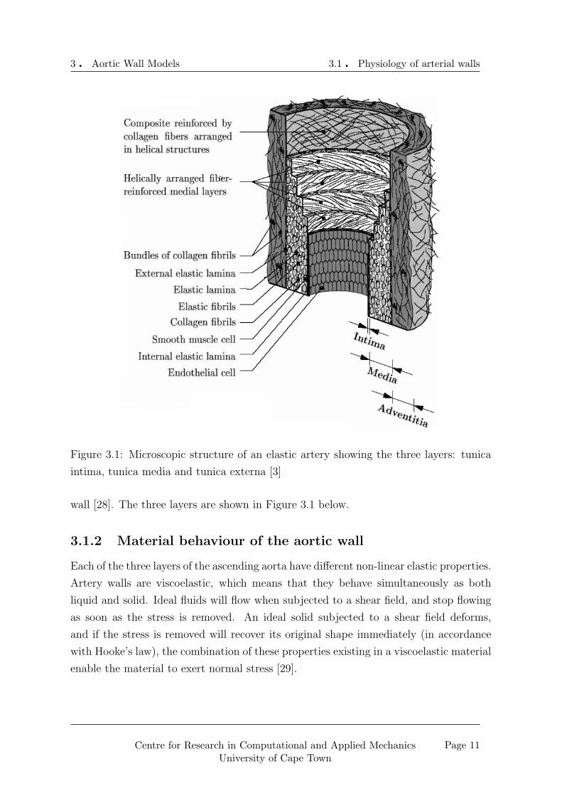
between 20 and 25mm along its length [26]. The aorta is made up of three layers, with
a combined (but not constant) thickness of approximately 2mm [27]. These three layers
of the aorta are common to all arteries in the body, but vary in size and thickness in
the different blood vessels. The innermost layer, the intima (tunica intima), is very thin
and almost negligible in a healthy young artery [3], the outermost layer, the adventitia
(tunica externa), makes up approximately one third of the total thickness, and the
middle layer, the media (tunica media), is the thickest portion of the ascending aortic
10
3 � Aortic Wall Models 3.1 � Physiology of arterial walls
Figure 3.1: Microscopic structure of an elastic artery showing the three layers: tunica
intima, tunica media and tunica externa [3]
wall [28]. The three layers are shown in Figure 3.1 below.
3.1.2 Material behaviour of the aortic wall
Each of the three layers of the ascending aorta have different non-linear elastic properties.
Artery walls are viscoelastic, which means that they behave simultaneously as both
liquid and solid. Ideal fluids will flow when subjected to a shear field, and stop flowing
as soon as the stress is removed. An ideal solid subjected to a shear field deforms,
and if the stress is removed will recover its original shape immediately (in accordance
with Hooke’s law), the combination of these properties existing in a viscoelastic material
enable the material to exert normal stress [29].
Page 11Centre for Research in Computational and Applied MechanicsUniversity of Cape Town

3 � Aortic Wall Models 3.1 � Physiology of arterial walls
Figure 3.2: Pressure-strain relationship of a healthy artery under loading. (Modified
from [4])
The elastic stiffness of arteries increases non-linearly as the load increases. At systole
(when the heart contracts) the arteries expand passively with blood, at diastole (when
the heart dilates) the arteries recoil elastically, causing the blood to be forced along the
arteries. This elastic recoil is the driving force of circulation and reduces the demand
on the heart to pump blood round the body. The particular non-linearity of the arterial
wall allows stable inflation of the vessel such that a small increase in pressure does not
cause a sudden large increase in radius [11]. The non-linear behaviour with loading of
a healthy artery is shown in Figure 3.2.
The three concentric layers of the arterial wall as discussed in Section 3.1.1 all ex-
hibit this non-linear behaviour, but with varying levels of stiffness. The innermost layer,
the intima, is the stiffest and the adventitia the least stiff of the three. The combined
properties of the layers are non-linear, and a certain degree of load transfer between the
layers results in the elastic recoil [11].
3.1.3 Mathematical model of the arterial wall
Various constitutive equations describing the material behaviour of soft, biological tis-
sues have been developed. For this investigation, the focus was on a model developed by
Page 12Centre for Research in Computational and Applied MechanicsUniversity of Cape Town

3 � Aortic Wall Models 3.1 � Physiology of arterial walls
Figure 3.3: Axis system for Holzapfel’s material model
Holzapfel [30]. Holzapfel’s model was based on the constitutive theory of finite hypere-
lasticity, combining neo-Hookean and Fung-type strain energy functions. The model was
developed from the results of uniaxial extension tests and histostructural data. These
tests were performed on the individual layers (intima, media and adventitia) of a healthy
human ascending aorta.
The mathematical model was of a transversely isotropic material. In uniaxial tension-
ing, the tensor in the direction normal to the plane becomes zero for an axis system as
in Figure 3.3.
The strain energy, Ψ, completely defines the material and is expressed as a function
of the Green-Lagrange strain tensor, E, and is made up of both an isotropic component
and a orthotropic component:
Ψ = Ψiso(ε) + Ψortho(ε). (3.1)
The isotropic component of the strain energy governs the initial stiffness of the artery,
while the orthotropic contribution governs the much higher stiffness at high strains.
Plane stress was assumed and therefore these components are functions of only E11 and
E22, yielding:
Ψ = Ψiso(ε11, ε22) + Ψortho(ε11, ε22) (3.2)
The Holzapfel model went on to assume incompressibility (ν = 0.5, where ν is
Poisson’s ratio). The isotropic component of strain energy is shown to be given by:
Ψortho =µ
22(ε11 + ε22) + [(2ε11 + 1)(2ε22 + 1)]−1 − 1 (3.3)
Page 13Centre for Research in Computational and Applied MechanicsUniversity of Cape Town

3 � Aortic Wall Models 3.1 � Physiology of arterial walls
The orthotropic contribution of the strain energy adopts a exponential “Fung-type”
strain energy function [31]. This incorporates four constitutive parameters C, c11, c12
and c22 where C is a stress-like parameter, while c11, c12 and c22 are dimensionless [31]
Thus,
Ψiso = C[eQ − 1] (3.4)
where:
Q = c11ε211 + c12ε11ε22 + c22ε
222 (3.5)
The stress then becomes:
σ11 =∂Ψ(ε11, ε22)
∂ε11
(3.6)
σ22 =∂Ψ(ε11, ε22)
∂ε22
(3.7)
and
σ33 = 0 (3.8)
The four constants (C, c11, c12 and c22) were obtained by a rigorous curve fitting process,
to yield the values shown in Table 3.1.
Layer µ (kPa) C (kPa) c11 c12 c22
Intima 39.8 1.42 999.0 510.0 127.0
Media 31.4 0.14 32.8 14.7 23.5
Adventitia 17.3 4.71E-04 37.7 58 63.8
Table 3.1: Material constants describing artery walls as derived by Holzapfel [30]
3.1.4 Effect of arteriosclerosis on the aorta
Age affects the arteries in a number of ways, and a condition known as arteriosclerosis
is often a result of the aging process. The main effect is a reduction in compliance
of the arteries due to a thickening of the intimal layer. As the intima has the stiffest
characteristics of the three layers (as can be seen in Table 3.1), thickening can drastically
reduce the arterial compliance. The result of this is that the elastic recoil as discussed
in Section 3.1.2 is less effective and there is a more substantial strain on the heart
muscle. Arteries may also become brittle with the aging process, increasing the chances
of rupture, which can occur during corrective surgery, sometimes having fatal results
[32].
Page 14Centre for Research in Computational and Applied MechanicsUniversity of Cape Town

3 � Aortic Wall Models 3.2 � Numerical models as used in this investigation
3.1.5 Compliance
Compliance is the percentage change in diameter of the artery for a pressure equivalent
to 100mmHg, thus it is a measure of elasticity of the artery. The mathematical formula
for compliance is:[33]
Cd =∆D
Dd∆P104. (3.9)
Compliance values in the ascending aorta range between 16.7%/100mmHg with an un-
certainty of ±84% [34] to 37%/100mmHg with an uncertainty of ±25% [35]. This large
range is due to different testing methods, but it is generally accepted to expect a com-
pliance value between 20% and 25% [32].
3.2 Numerical models as used in this investigation
For each model the geometry, material parameters and boundary conditions and surface
interactions of the models will be described in the following sections. Any aspects specific
to the individual models will be further explained in the corresponding section.
3.2.1 Common geometrical aspects
The ascending aorta was simplified to resemble a straight cylinder, and therefore the
entire problem was assumed to be axi-symmetric. The cylinder had a length (parallel
to the flow direction) of 50mm and an internal diameter of 12.05mm. This diameter
corresponded with the geometrical condition at diastole. This simple geometrical offset
acted as the pre-tension in the aorta, which was sufficient as the material was modelled
as linearly elastic throughout and therefore independant of the deformation history.
The initial thicknesses of the media and adventitia were set at 1.2mm and 0.6mm
respectively, thus the combined thickness of the two layers was 1.8mm in agreement
with Gao’s model [16]. The geometry is shown in Figure 3.4
3.2.2 Boundary conditions and surface interactions
Boundary conditions fix certain motion or applied tractions, while interactions specify
contact relationships between two components or materials. In the models, the only
type of interaction used was the elastic foundation, which was used to model the effects
of surrounding fatty and muscular tissue. This acts as a series of springs, in parallel,
along the length of the relevant surface with a stiffness per unit area, (k/A) specified
Page 15Centre for Research in Computational and Applied MechanicsUniversity of Cape Town

3 � Aortic Wall Models 3.2 � Numerical models as used in this investigation
Figure 3.4: Geometry of modelled ascending aorta
by the user. These springs approximate another material or deformable part in direct
contact with the modelled solid. The stiffnesses were evaluated as follows:
For linear elasticity
E =σ
ε
where σ = FA
and ε = ∆LLinit
, thus:
E =FLinit
A∆L
but, according to Hooke’s law
k =F
∆L
therefore
E =kLinit
A
and thus the stiffness per unit area:
k/A =E
Linit
(3.10)
The boundary conditions and surface interactions for the models are as follows:
1. At inlet:
No displacement was allowed in the axial direction (uz = 0)
No rotation was allowed in the circumferential direction (θz = 0)
Page 16Centre for Research in Computational and Applied MechanicsUniversity of Cape Town

3 � Aortic Wall Models 3.2 � Numerical models as used in this investigation
2. At outlet:
An elastic foundation was specified, such that the ascending aorta may “shorten”
but not freely, with the stiffness per area such that it was equivalent to there being
50mm of aortic material extending from it.
3. Along the length of the aorta:
Two different elastic foundations were specified along the length of the aorta, for
1mm, k/A = 8000Pa/m2 and for the rest of the length k/A = 4000Pa/m2.
The inlet condition constrains the aortic model where it was “connected” to the left
ventricle, and assumed that the area in direct contact would not move away from the
ventricle (condition 1).
The interaction acting on the first 1mm after inlet to the aorta (as mentioned in con-
dition 3) acted as a cylinder encompassing the beginning of the aorta, allowing it to
expand in a constrained fashion.
The outlet of the ascending aorta model was allowed to move in any direction (con-
dition 2), but was restrained from an uncontrolled axial shortening by an interaction
mimicking an extension of aortic material for 50mm, which was the modelled aorta
length again. This interaction was specified to mimic, to some extent, the support of
the aortic arch, descending aorta and the rest of the system.
As the aorta is supported by various biological tissues and fluids within the my-
ocardium, the model needed to be constrained along its length in some way (condition
3). The combination of these media were approximated as a 2.5mm thick layer of fat,
following the example set out by Janoske et al [8].
The layers of the aorta were modelled as one entity, with the total thickness partitioned
into layers with material properties specific to the relevant sections of the aorta (intima,
media and adventitia), rather than separate parts modelled in full contact with one
another. This modelling technique was used to ensure that any deformation of the
vessel did not cause any separation between the layers as a result of the soft and hard
contact methods of employed by ABAQUS R© . For the hard contact specification, the
penetration of one surface into the other is minimised, and as soon as the contact
pressure reduces to zero, the surfaces will separate. This presents the risk of a loss of
contact. When soft contact is specified, a force exists between the surfaces as a function
of the distance between the surfaces. Because this force exists, actual contact between
Page 17Centre for Research in Computational and Applied MechanicsUniversity of Cape Town

3 � Aortic Wall Models 3.2 � Numerical models as used in this investigation
the surfaces may never actually occur. Using an elastic foundation also obviates the
existence of two deformable parts, and consequently two meshes, thus simplifying the
solution of the matrix. The boundary conditions are shown in Figure 3.5.
3.2.3 Loading conditions on the aorta
As previously discussed, the aorta was modelled during diastole, therefore for the inde-
pendantly run solid simulations only the difference in pressure from diastole to systole
(equivalent to 40mmHg) was applied to the aorta. This load was applied as a uniform
pressure along the entire inner wall of the artery creating the condition as shown in
Figure 3.5.
For the coupled simulations the loading is as described in Chapter 5.
3.2.4 Development of constitutive equations
As previously discussed blood vessels are viscoelastic (see Section 3.1.2), in this investi-
gation, the ascending aorta was analysed within the linear range of elasticity. The ma-
terial model was obtained by the linearisation of the constitutive equations as discussed
in Section 3.1.3 which takes the transverse isotropic nature of arteries into account.
The model discussed in Section 3.1.3, described the strain energy, Ψ, as consisting of
the sum of two components, one isotropic, Ψiso(ε), and one orthotropic, Ψortho(ε). The
material was approximated as being incompressible (ν = 0.5), and the model defined
a hyperelastic material, however, for a linear elastic model, material stability requires
that the tensor Del be positive definite and thus there exist certain restrictions on the
material constants.
The assumption of incompressibility led to this instability and therefore the material
was instead modelled as being near-incompressible, with ν = 0.45.
The isotropic component from the Holzapfel model was discarded and was instead de-
veloped incorporating the Lame moduli, where:
λ =Eν
(1 + ν)(1− 2ν)(3.11)
and
µ =E
2(1 + ν)(3.12)
It can be seen from Equation 3.11 how the assumption of incompressibility lead to a
zero denominator in λ and why the near-incompressible model was necessary.
Page 18Centre for Research in Computational and Applied MechanicsUniversity of Cape Town

3 � Aortic Wall Models 3.2 � Numerical models as used in this investigation
Figure 3.5: Boundary conditions, surface interactions and loading conditions on the
models
Page 19Centre for Research in Computational and Applied MechanicsUniversity of Cape Town

3 � Aortic Wall Models 3.2 � Numerical models as used in this investigation
Thus the isotropic stress component of the material, as a function of strain, was:
σ = λ(E11 + E22 + E33)(I) + 2µ((E) (3.13)
where (I) is the identity matrix.
The orthotropic component of Holzapfel’s model was linearised via a Taylor expansion
to the first degree, and added to the above isotropic component. The linearisation led
to the following stress definitions:
σ11 = σ11(0) + α11ε11 + α22ε22 (3.14)
σ22 = σ11(0) + β11ε11 + β22ε22 (3.15)
where
α11 =∂σ11
∂ε11
∣∣∣∣0
(3.16)
α22 =∂σ11
∂ε22
∣∣∣∣0
(3.17)
β11 =∂σ22
∂ε11
∣∣∣∣0
(3.18)
β22 =∂σ22
∂ε11
∣∣∣∣0
(3.19)
and
σ11 =∂Ψ
∂ε11
(3.20)
σ22 =∂Ψ
∂ε22
∣∣∣∣0
(3.21)
This gives:
α11 = 4µ + 2c11C (3.22)
α22 = 2µ + Cc12 = β11 (3.23)
β22 = 4µ + 2c22C (3.24)
The components were transformed into an equivalent cylindrical coordinate system
such that the subscripts 1, 2 and 3 are equivalent to r, z and θ respectively and summed
Page 20Centre for Research in Computational and Applied MechanicsUniversity of Cape Town

3 � Aortic Wall Models 3.2 � Numerical models as used in this investigation
to give
σrr
σzz
σθθ
τrz
τrθ
τzθ
= [D]
εrr
εzz
εθθ
γrz
γrθ
γzθ
(3.25)
where:
[D] =
α11 + λ + 2µ α22 + λ λ 0 0 0
β11 + λ β22 + λ + 2µ λ 0 0 0
λ λ λ + 2µ 0 0 0
0 0 0 2µ 0 0
0 0 0 0 2µ 0
0 0 0 0 0 2µ
MPa (3.26)
The constants were dealt with in a way specific to each model, which will be discussed
in the sections on the individual models.
3.2.5 Meshing of the models
The models were all meshed in the same manner as they all needed to be compatible
with the fluid model mesh. It was necessary that the mesh be fine enough to capture
any relevant information in the running of the job. On the other hand an excessively fine
mesh was avoided so as to keep the compatibility of the fluid and solid grids as simple
as possible. It was found that 200 elements along the common boundary was sufficient
for this problem, with an equivalent spacing along the two boundaries perpendicular
to the axis of symmetry. This resulted in 0.25mm spacing between the nodes. A free
meshing technique was adopted, as it was found that this allowed the greatest control
according to the edge seeding. The meshed part is shown in the section specific to the
individual model. The elements used were axisymmetric stress elements, which is the
default element type for axisymmetric models in ABAQUS R© . This element type allows
only isotropic or orthotropic material properties, and loading only in the radial and axial
directions. If a radial displacement occurs, this will cause a “hoop” strain, which is a
strain in the circumferential direction.
Page 21Centre for Research in Computational and Applied MechanicsUniversity of Cape Town

3 � Aortic Wall Models 3.2 � Numerical models as used in this investigation
3.2.6 Models of a healthy, young ascending aorta
In a healthy artery the intima is “very thin” [3] and thus the effect of this layer on
the solid mechanical properties is assumed to be insignificant. Consequently the models
analysed in this subsection neglected this layer entirely, with only the material and
geometrical properties of the media and adventitia being included.
Single layer, isotropic model
Geometry: The geometry of the aorta is that shown in Figure 3.4, with the combined
thickness of the two relevant layers used as the entire wall thickness (1.8 mm). The
ascending aorta model is five centimetres long with an internal diameter of 12.5 mm as
used in [16].
Material: The first model created was linear elastic, isotropic and consisted of only a
single layer. The elastic modulus of this layer was derived as a weighted average of the
elastic moduli found for the two layers, according to the area of each of the layers in the
cross section of the ascending aorta as follows:
Eave =2
3Emedia +
1
3Eadventitia (3.27)
as the media makes up two thirds and the adventitia makes up one third of the total
cross sectional area of the ascending aorta (see Figure 3.6 in Section 3.2.6), and E was
found from Equation 3.12.
As the material is isotropic, the constants in the orthotropic component of the math-
ematical model were set to zero:
c11 = c12 = c22 = 0 (3.28)
while all the others were maintained as those in Table 3.1. The elastic modulus of the
isotropic material was 0.07794MPa and had a D-matrix of:
[D] =
0.2937 0.2403 0.2403 0 0 0
0.2403 0.2937 0.2403 0 0 0
0.2403 0.2403 0.2937 0 0 0
0 0 0 0.0534 0 0
0 0 0 0 0.0534 0
0 0 0 0 0 0.0534
MPa (3.29)
Page 22Centre for Research in Computational and Applied MechanicsUniversity of Cape Town

3 � Aortic Wall Models 3.2 � Numerical models as used in this investigation
Figure 3.6: Cross section of healthy artery showing the thicknesses of the medial and
adventitial layers
Boundary conditions and surface interactions: The boundary conditions de-
scribed in Section 3.2.2 hold for this model. The elastic foundation at the aortic outlet
has a stiffness per area of 1548.6Pa/m2, which represents a continuation of the material
properties as for the rest of this model. The interaction property values in all other
regions of the model are as set out in Section 3.2.2.
Double layer, isotropic model
Geometry: This model consisted of two layers; the media, being 1.2mm thick, and
the adventitia, being 0.6mm thick. All geometrical aspects of this model are as discussed
in Section 3.2.1 and the cross section is shown in Figure 3.6.
Material: As in the single layer, isotropic model (Section 3.2.6), the material model
was isotropic. Therefore the constants in the orthotropic component of the material
model were zeroed:
c11 = c12 = c22 = 0 (3.30)
Page 23Centre for Research in Computational and Applied MechanicsUniversity of Cape Town

3 � Aortic Wall Models 3.2 � Numerical models as used in this investigation
for all of the layers. The various material constants are shown in Table 3.1, and were
assigned to the relevant layers, yeilding a D-matrix as follows:
[D] =
0.3454 0.2826 0.2826 0 0 0
0.2826 0.3454 0.2826 0 0 0
0.2826 0.2826 0.3454 0 0 0
0 0 0 0.0628 0 0
0 0 0 0 0.0628 0
0 0 0 0 0 0.0628
MPa (3.31)
for the medial layer, with E = 0.09106Mpa, and
[D] =
0.1903 0.1557 0.1557 0 0 0
0.1557 0.1903 0.1557 0 0 0
0.1557 0.1557 0.1903 0 0 0
0 0 0 0.0346 0 0
0 0 0 0 0.0346 0
0 0 0 0 0 0.0346
MPa (3.32)
for the adventitial layer, with E = 0.0517.
Boundary conditions and surface interactions: Once again the elastic models as
described in Section 3.2.2 held. The elastic foundation at the outlet was specific to each
layer of the aorta, with an extension of the media tissue connecting to the medial layer
at outlet and an extension of the adventitia tissue connecting to the adventitial layer
at outlet. This resulted in k/A = 1821.2Pa at the media and k/A = 1034Pa at the
adventitia. All other interaction properties from Section 3.2.2 held..
Double layer, orthotropic model
Geometry: As in section 3.2.6 the model consisted of two layers, as shown in Figure
3.6. The media is once again 1.2mm thick and the adventitia 0.6mm thick.
Material: The material in this model is orthotropic, with the values of the constants
mentioned in section 3.1.2 having the values shown in Table 3.1.
Page 24Centre for Research in Computational and Applied MechanicsUniversity of Cape Town

3 � Aortic Wall Models 3.2 � Numerical models as used in this investigation
These values result in a D-matrix of:
[D] =
0.345400 0.282600 0.282600 0 0 0
0.282600 0.354584 0.284658 0 0 0
0.282600 0.284658 0.351980 0 0 0
0 0 0 0.062800 0 0
0 0 0 0 0.062800 0
0 0 0 0 0 0.062800
MPa (3.33)
for the medial layer, with E = 0.03106Mpa and
[D] =
0.190300 0.155700 0.155700 0 0 0
0.155700 0.190360 0.155727 0 0 0
0.155700 0.155727 0.190335 0 0 0
0 0 0 0.034600 0 0
0 0 0 0 0.034600 0
0 0 0 0 0 0.034600
MPa (3.34)
for the adventitial layer, with E = 0.0517MPa.
Boundary conditions and surface interactions: Again the boundary conditions
and interactions as laid out in Section 3.2.2 hold. The interaction property values are
the same as those discussed in Section 3.2.6 above.
3.2.7 Models of an aged/diseased artery
Effects of age and disease
As dicussed in section 3.1.4, arteriosclerosis is caused by a thickening of the intimal layer
in the arteries. As the elastic properties of the intima lead to a much stiffer material, this
thickening reduces compliance in the arteries. This effect was investigated by adding an
intimal layer to the wall model as described in the sections below.
It should be noted that the effects of atherosclerosis would be similar to those of arte-
riosclerosis, at some level, as the former is a build up of various compounds (cholesterol,
calcium, etc), which also cause a stiffening of the artery walls. However, this condition
also “clogs” the artery, decreasing the cross sectional area through which the blood must
flow, thus further increasing the strain on the heart.
Page 25Centre for Research in Computational and Applied MechanicsUniversity of Cape Town

3 � Aortic Wall Models 3.2 � Numerical models as used in this investigation
Figure 3.7: Cross section of model affected by arteriosclerosis, with an initial intimal
thickening of 0.2mm
Geometry: The model of the artery affected by arteriosclerosis included all three lay-
ers; intima, media and adventitia. The inner diameter of the aorta was held at 12.05mm
to maintain compatibility with the fluid mesh, while the outer diameter became larger
as a result of the increasing thickness of the artery wall. The initial model had an in-
tima with a thickness of 0.2mm (as used by Gao et al [16] in a three layer healthy aorta
model). The thickness was increased to 0.4mm and finally to 0.6mm, at which point
it has the same thickness as the adventitia, to investigate the possible existence of a
trend with intimal thickening. Figure 3.7 shows the first model, with the initial intimal
thickening condition.
Material: The material model for the medial and adventitial layers was the same as
that in Section 3.2.6. The added intimal layer used the constants as shown in Table 3.1
and E = 0.11542MPa. The D-matrix for the two outer layers were as in Section 3.2.6,
Page 26Centre for Research in Computational and Applied MechanicsUniversity of Cape Town

3 � Aortic Wall Models 3.2 � Numerical models as used in this investigation
while that of the intimal layer was:
[D] =
0.437800 0.358200 0.358200 0 0 0
0.358200 0.288094 0.760020 0 0 0
0.358200 0.760020 0.404460 0 0 0
0 0 0 0.079600 0 0
0 0 0 0 0.079600 0
0 0 0 0 0 0.079600
MPa (3.35)
.
Boundary conditions and surface interactions: The boundary conditions and
surface interactions as described in Section 3.2.2 held, with the elastic foundation at the
outlet being that of each layer extending for 50mm. The surface interaction properties
for the media and adventitia at outlet were the same as those in Sections 3.2.6 and 3.2.6.
The intima outlet interaction had a value of k/A = 2308.4Pa.
Page 27Centre for Research in Computational and Applied MechanicsUniversity of Cape Town

Chapter 4
Blood Flow Models
A single blood flow model was developed and used for every wall model. The details of
the modelling process will be laid out in this chapter, introduced by a review of literature
on the subject. The modelling process is then described in the following sections.
4.1 Blood flow in the ascending aorta
Blood is a very complex fluid, and the pulsatile nature of blood flow in the human
body adds still more complexity to the modelling of this flow, however there are various
assumptions which may be made to greatly simplify this problem.
4.1.1 The material properties of blood
Blood is a non-Newtonian fluid, a class of fluids including all fluids that have behaviour
deviating from Newton’s laws. In a Newtonian fluid, the rate of deformation of the fluid
and the stress applied to it are directly proportional, that is, the fluid obeys Newton’s
law of constant viscosity. A non-Newtonian fluid, like blood, has a non-linear response
to stress; the stress in the fluid is dependant on both the instantaneous deformation
and the instantaneous rate of change of the deformation [29]. This greatly affects the
behaviour of blood in arteries, however it is reasonable to model blood as a Newtonian
fluid when dealing with large, elastic arteries [24] and, as the aorta is the largest artery
in the human body, this assumption applied to this investigation.
28

4 � Blood Flow Models 4.2 � Grid geometry and boundary conditions
4.1.2 Blood flow characteristics
Flow in arteries is pulsatile, which may cause the flow to become turbulent, thus an
investigation into this possibility was conducted by Morris et al [24]. Accelerating flow
is more stable and decelerating flow less stable than steady flow, therefore there is a
possibility of bursts of turbulence in the decelerating phase of the pressure pulse [36],
[37]. In another investigation, conducted by Nerem et al [38], a critical Reynolds number
for unsteady flow was found. For the model used by Morris et al [24] the maximum
Reynolds number (for the decelerating flow phase) was below this critical value and
thus the flow was assumed to be laminar.
4.1.3 Laminar flow
When a fluid flows along a surface the friction between the surface and the fluid causes
there to be no relative motion between the surface and the fluid that is in direct contact
with it. As a result of this, a velocity gradient exists between the fluid at the surface
and the fluid far away from the surface (i.e. that in the free stream). In fully developed
pipe flow the flow profile approximates a parabola, due to the increasing velocity with
distance from the wall, and the shape of this parabola is determined by the viscosity of
the fluid.
4.2 Grid geometry and boundary conditions
As the ascending aorta was approximated as cylindrical, with a constant cross section,
the flow was assumed to be axi-symmetric. FLUENT R© calculates the results of axi-
symmetric problems by integrating over 2Π radians. The geometry for the flow domain
of the aorta was defined in GAMBIT R© . A rectangular domain was created and meshed,
as shown in Figure 4.1.
Four boundary types were assigned as follows:
• The common boundary between the solid and fluid meshes was defined as a “wall”
boundary, which contains the fluid and defaults to a no slip condition.
• The centre line of the aorta was defined as an “axis” boundary, which assigns it
axis of symmetry properties, and does not require the specification of any other
boundary conditions.
Page 29Centre for Research in Computational and Applied MechanicsUniversity of Cape Town

4 � Blood Flow Models 4.3 � General properties of model
Figure 4.1: Meshed grid used for CFD analysis
• The inlet boundary was assigned a “velocity inlet” boundary type as the informa-
tion available described an inlet value [24]. This type of boundary is suitable for
incompressible flow. The inlet velocity profile will be described in section 4.6.
• At the outlet, no information was known, and therefore an “outflow” boundary
type was assigned, which is also appropriate for incompressible flow. For this type
of boundary, FLUENT R© extrapolates the required information from the interior.
• The fluid within the boundaries assumed the default “interior” boundary type.
The mesh consisted of bilinear quadrilateral elements, created by the “map” meshing
scheme, which creates a structured, regular grid. The grid was refined in the area close
to the artery wall so as to monitor boundary layer phenomena. The refinement was
graded according to an exponential function with a ratio value of 0.32. A total of 40
elements were created along the inlet and outlet boundaries of the aorta. The elements
along the wall and axis boundaries were evenly spaced for 200 elements.
As discussed in Section 3.2.5 it was essential to have a grid fine enough to capture any
relevant flow phenomena but also it was necessary to maintain compatibility with the
solid mesh. The nodes on the fluid domain wall boundary fell on the same points as the
nodes on the solid boundary.
4.3 General properties of model
As discussed in Section 4.1, blood flowing through the aorta can be approximated as
Newtonian, therefore, the density and viscosity were set as constant, with values of
Page 30Centre for Research in Computational and Applied MechanicsUniversity of Cape Town

4 � Blood Flow Models 4.4 � Operating Conditions
1050kg/m3 and 0.0035Pas respectively and the fluid was assumed incompressible [16],
[24].
4.4 Operating Conditions
Due to the fact that the wall model had an initial condition of diastolic pressure, the
initial pressure induced in the artery had to be representative of the flow conditions at
systole. Therefore the operating conditions were set at the systolic condition, with an
operating (guage) pressure of 120mmHg. The reference point was set at the inlet to the
aorta at the vessel wall (i.e. on the common boundary).
4.5 Flow characteristics as defined in Fluent
The flow was defined as axi-symmetric, and therefore an axi-symmetric solver was
utilised. A time averaged input velocity as deduced by Morris et al [24] was applied.
This inlet velocity was deduced from flow rates obtained from Nichols and Rourke [39].
As discussed in 4.1, the model used by Morris et al [24] was laminar for the decelerating
phase of the flow, therefore as steady flow is more stable than flow in the decelerating
phase [36], the flow was assumed to be laminar throughout the ascending aorta.
The working fluid was set as blood with the properties discussed in Section 4.3. The
default no slip condition at the aorta wall was retained. At the outflow boundary the
flow rate weighting was left at the default value of 1, as all the flow exits through the
same outlet.
4.5.1 Solution Controls
SIMPLEC (Semi-Implicit Method for Pressure-Linked Equations (Consistent)) was used
as the method of pressure velocity coupling and the under-relaxation factors were left
at the default values. This solver is an improved version of the SIMPLE algorithm and
is ideal for steady state problems [40]. The discretisation scheme utilised was QUICK
(Quasi-upwind interpolation for convective kinetics), which interpolates between three
data points with an upstream weighting [24]. The increased accuracy due to the extra
data point was not foreseen to create any significantly increase the simulation time due
to the computational simplicity of the model.
Page 31Centre for Research in Computational and Applied MechanicsUniversity of Cape Town

4 � Blood Flow Models 4.6 � Investigation into the inlet velocity profile
Figure 4.2: Partitions and mesh of investigated inlet velocity profile
4.6 Investigation into the inlet velocity profile
Blood flow into the ascending aorta is controlled by a one-way valve (the aortic valve).
The change in flow area from the left ventricle of the heart to the ascending aorta was
foreseen to yield a velocity profile at the aorta inlet which was neither completely flat
nor parabolic (the case in fully developed laminar flow (see Section 4.1)).
This combination of velocity gradients was expected as a result of the sudden change in
flow area, but the extent of the gradients was not known quantitively. However, it was
expected, from reports of CT scans [36], [41],[42], [43], [44] that the profile would show
a relatively flat velocity profile at the inlet to the aorta.
4.6.1 Geometry and mesh
The geometry of the aorta with the included ventricle is shown in Figure 4.2. The
geometric properties of the aorta are the same as those described in Section 4.2. The
extension of the left ventricle is by no means an accurate representation, but merely
served the purpose of simulating a sudden change in flow area. The radius of the
ventricular section was set to five times that of the aorta radius, at 60.25mm. The
section connecting the ventricle to the aorta was angled at 30◦, and entry was smoothed
with a fillet radius of 3.95mm (see Figure 4.2).
Page 32Centre for Research in Computational and Applied MechanicsUniversity of Cape Town

4 � Blood Flow Models 4.6 � Investigation into the inlet velocity profile
The rectangular aortic section was meshed as described in Section 4.2. The ventricle
was partitioned as shown in Figure 4.2, to allow the most even mesh possible. Parts 2 and
3 (Figure 4.2)) essentially extend the mesh from Part 1, with an exponentially graded
mesh, in keeping with that of Part 1. Due to the quadrilateral shape of these parts,
they were meshed with the “map” meshing scheme of GAMBIT R© with quadrilateral
elements.
It was not imperative that the elements along the inlet boundary of Part 4 were graded
as they are sufficiently far away from any surface. 41 evenly spaced elements were set
along this edge, and 52 along the axis boundary (which were extended through Part
3). As this section was three sided, GAMBIT R© ’s “tri-primitive” meshing scheme was
utilised. This scheme divides a three sided shape into three quadrilateral regions and
uses a “map” scheme to mesh these three regions [40]. A total of 15008 elements were
created for this model.
4.6.2 Boundary conditions
The boundary conditions as described in Section 4.2 were applied to the model, except
for those at the inlet to the aorta. The inlet to the “ventricle” was assigned the velocity
inlet boundary type and the inlet to the aorta/outlet to ventricle was defined as an
interior boundary type, to enable the extraction of data at this boundary. The ventricle
wall was assigned the wall boundary type and the no slip condition was retained.
Inlet condition
The profile was investigated with a crude geometric model of the left vetricle leading
into the diameter of the aorta as shown in Figure 4.2. The average axial velocity at inlet
to the aorta was approximated as 0.0035m/s [24]. This condition was ensured by the
assumption of a constant volume flow rate to the ventricle inlet as shown in Figure 4.2.
Continuity in an incompressible fluid is satisfied by:
vinAin = voutAout (4.1)
where A is the cross-sectional flow area and v is the velocity normal to A, while subscripts
“in” and “out” are the values at inlet and outlet respectively, this resulted in a constant
velocity value of 0.00354m/s at the “inlet” to the ventricle.
Page 33Centre for Research in Computational and Applied MechanicsUniversity of Cape Town

4 � Blood Flow Models 4.6 � Investigation into the inlet velocity profile
4.6.3 Use of profile in final model
The model was run with the flow characteristics as defined in Section 4.5 and the ve-
locity profile was extracted at the aortic inlet. This profile was then programmed into
a User Defined Function (U.D.F) which was included in the boundary condition at the
aorta inlet in the final model.
FLUENT R© requires that the velocity be given as a function (written in the C program-
ming language) such that any value of velocity at any point on the boundary of interest
may be determined. The U.D.F. is included below:
vprofile.c
UDF for specifying steady-state velocity profile boundary condition
************************************************************************/
#include "udf.h"
DEFINE_PROFILE(inlet_x_velocity, thread, position)
{
real x[ND_ND]; /* this will hold the position vector */
/*real z = 0;*/
face_t f;
int i, n;
real R[31], V[31], v;
FILE *fp;
fp = fopen("RvsV_vectors.txt", "r");
n = 30; /*counter maximum*/
for (i=0; i<=n; i++)
{fscanf(fp, "%f%f", &R[i], &V[i]);
}
begin_f_loop(f, thread)
{
F_CENTROID(x,f,thread);
for (i=0; i<=(n-1); i++)
{
if (x[1]>=R[i] & x[1]<R[i+1])
Page 34Centre for Research in Computational and Applied MechanicsUniversity of Cape Town

4 � Blood Flow Models 4.6 � Investigation into the inlet velocity profile
{
v = V[i] + ((V[i+1]-V[i])/(R[i+1]-R[i]))*(x[1]-R[i]);
}
}
F_PROFILE(f, thread, position) = v;
}
end_f_loop(f, thread)
fclose(fp);
This U.D.F. initialises two arrays, one containing the node values in the range of the
inlet, and the other the axial velocity magnitudes at these nodes. Because the nodes
are close together, a simple linear interpolation between nodes was specified to smooth
the function, such that:
v =∆v1−2
∆r1−2
r + v1 (4.2)
Where v is the velocity, r is the radius, subscripts 1 − 2 are the change between the
consecutive known values, and subscript 1 is the previous known value.
Note on inlet velocity profile
It must be noted that due to the fact that the same velocities at inlet are used in spite
of the inlet area changing, the volume flow rate will not be constant. However, it was
expected that due to the extra constraints of the aorta at the inlet (see Section 3.2.2),
the radial displacements of the ascending aorta would not cause an appreciable change
in flow area. This was investigated and found to be the case (see Section 6.1), and the
method was applied as described above.
Page 35Centre for Research in Computational and Applied MechanicsUniversity of Cape Town

Chapter 5
Interface and Coupling
This chapter explains the coupling process used in this investigation. The interface
between the solid problem (in ABAQUS R© ) and the fluid problem (in FLUENT R© )
was written in the Matlab programming language and the code is included on the
CD attached to this report. Principles upon which the the code was based, various
algorithms used, and the purposes of each programme will be described in this chapter,
preceeded by an introduction to the theory behind coupling.
5.1 What are coupled systems?
The aim of the investigation was to simulate the coupling between the solid and fluid
problems in the ascending aorta. A coupled system is one consisting of at least two
distinct systems, which overlap with common variables. Although each system is solved
with a characteristic set of differential equations, the overlapping variables make it
impossible to solve each system separately [5] and information has to be exchanged
between the systems to fully solve the problem. Figure 5.1, shows the basics of a
coupled system.
5.2 Coupling as applied to this study
The system in this investigation is the fluid structure interaction (FSI), and the common
variables are displacement and pressure. The fluid problem is solved by the Navier-
Stokes equations (see Section 2.2) and the solid probelm is solved for solid equilibrium
(see Section 2.1). ABAQUS R© and FLUENT R© do not perform this coupling automati-
cally.
36

5 � Interface and Coupling 5.2 � Coupling as applied to this study
Figure 5.1: A coupled system showing two domains and a coupling region. Variables c
and d are shared in the system. (courtesy of [5])
The fluid flow creates a pressure profile on the aortic wall, causing the structure to
deform. The displacements of the solid boundary consequently cause a change in the
flow, creating a new pressure profile, in turn changing the geometry of the boundary wall
once again. In the steady flow scenario specific to this investigation, this continued to
happen until an equilibrium was reached between the aortic wall and the blood flowing
in the aorta.
The way the problem ran is as follows:
1. Blood flow was simulated and a pressure profile on the boundary was output.
2. The pressure profile was applied to the aortic wall outputting displacement values
of the wall.
3. The new fluid domain boundary coordinates were aquired and a new flow domain
defined.
The system repeated itself until equilibrium was reached.
5.2.1 Exchanged variables
The pressure profile required from the fluid system was that of total pressure at the
common boundary, which is the sum of the static and dynamic pressures [45]:
Total pressure = ∆p︸︷︷︸static pressure
+ 12ρv2︸︷︷︸
dynamic pressure
The deformations required from the solid system were the nodal displacements at the
common boundary.
Page 37Centre for Research in Computational and Applied MechanicsUniversity of Cape Town

5 � Interface and Coupling 5.3 � Available software for coupling problems
Figure 5.2: Initial exchange of data and subsequent parallel solving as used by MpCCI
(courtesy of [5])
5.3 Available software for coupling problems
Mesh based Parallel Code Coupling Interface (MpCCI R© ) is a software designed to han-
dle a range of coupling processes including the FSI as described in the above sections.
MpCCI R© searches the relevant input files for regions which exhibit coupling compati-
bility. This software uses a weak coupling system (that in which each system is solved
separately) to solve the problem. MpCCI R© runs a parallel solution that runs as shown
in Figure 5.2.
The use of this software would have allowed a more complex model in this inves
tigation as described in Section 1.2.
5.4 Sequence used for running the coupled simula-
tion
The interface as created in this investigation minimised the requirement for manual data
transfer as far as possible, however, in order to allow the process to be monitored and
evaluated, the process was run in a series of steps. These steps are set out in the fol-
lowing flow chart (Figure 5.3) and each step is described in the following subsections of
this chapter. For better clarity in the following sections, example files of the ABAQUS R©
input and data files as well as the FLUENT R© case files have been included along with
the programming code on the CD attached to this document.
Page 38Centre for Research in Computational and Applied MechanicsUniversity of Cape Town

5 � Interface and Coupling 5.4 � Sequence used for running the coupled simulation
Figure 5.3: Flow chart showing the sequence of actions required to run a coupled simu-
lation as defined in this investigation.
Page 39Centre for Research in Computational and Applied MechanicsUniversity of Cape Town
5 � Interface and Coupling 5.4 � Sequence used for running the coupled simulation
It should be noted, before describing any of the code, that when an axi-symmetric
problem is specified in ABAQUS R© , the Y-axis is the convention for the axis of symmetry,
whereas FLUENT R© uses the X-axis as the axis of symmetry. Therefore all coordinate
systems were transformed accordingly.
5.4.1 Files required in working directory
For the simulation to run correctly, the following nine files needed to exist in the current
working directory:
1. Pre Fluent1.m
2. Initial FLUENT R© case file, with the extension .cas
3. Pre Abaqus1.m
4. Initial ABAQUS R© input file, with the extension .inp. This file should not have a
defined load and necessary changes as described in the corresponding section must
be made.
5. AfterAbaqus.m with initial file names
6. AfterFluent.m
7. profile.c
8. journal temp.txt
9. RvsVtemp.txt
5.4.2 Pre Fluent1.m
Creation of journal file
This programme creates a journal file to be read by FLUENT R© . A journal file (ex-
tension .jou) contains certain instructions which FLUENT R© reads and executes. These
commands are the same as those which can be typed directly into the FLUENT R© console
to perform the required actions. The journal file created by Pre Fluent.m commands
FLUENT R© to extract the profile of total pressure and write it to a text file (extension
.xy) which is given a standard name, and placed in the working directory.
The journal file is created from the template text file, named journal temp.txt. The
Page 40Centre for Research in Computational and Applied MechanicsUniversity of Cape Town

5 � Interface and Coupling 5.4 � Sequence used for running the coupled simulation
additional information which Pre Fluent1.m writes to the journal is the name of the
pressure profile file to be created.
Creation of U.D.F reference file
The U.D.F. used for the velocity profile at the inlet to the aorta calls an array of the
coordinates along the inlet boundary. Because it was expected that the range of the
inlet would change and thus the array would have to be updated for U.D.F. to call the
correct r values for each simulation. Pre Fluent1.m creates the initial range for the
U.D.F (profile.c) to read. The text file RvsVtemp.txt contains the template of initial
coordinate values to be used.
Boundary node extraction
Because the nodes of interest are only those at the common boundary between fluid
and solid, it was necessary to distinguish these from the rest of the nodes. A vector is
created by Pre Fluent1.m, which is then used by the subsequently run programmes, as
the node numbering does not change, but the node coordinates corresponding to these
numbers do.
This was acheived via a loop containing a condition forcing only the nodes along the
common boundary to be placed into the vector. These nodes were then arranged in the
ascending order of the node numbers.
Boundary element extraction
As an element set was defined in ABAQUS R© for the inner wall of the aorta, these
elements were listed in the input file (extension .inp) and were simply extracted and
placed in a vector. In case of this element set not being defined in ABAQUS R© , or if
the input file is formatted without CAE (the user interface of ABAQUS R© ), a loop was
created which can extract these elements on the condition that the nodes constituting
the four element corners includes at least one of the node numbers in the boundary node
vector as detailed in the above section.
5.4.3 Initial flow model case file
It was important that the same case file was used for all the models. The solver con-
ditions may be altered but the grid formation (as created in GAMBIT R© ) had to come
from the same file every time. The reason for this was that when a grid is created, the
Page 41Centre for Research in Computational and Applied MechanicsUniversity of Cape Town

5 � Interface and Coupling 5.4 � Sequence used for running the coupled simulation
bandwith of the solution matrix is optimised. Therefore, the nodes are numbered in an
order specific to each model. The node connectivity as defined in the case file is written
in a hexadecimal numbering system, which makes it complicated to analyse. It is con-
sequently simpler to ensure that the same node numbering and thus the corresponding
node connectivity is used for every model, to be compatible with the programming code
creating the new case file for the subsequent job.
An unfortunate result of this is that the written code became very problem specific,
and cannot be used generally for any rectangular grid created in GAMBIT R© . Notwith-
standing this, the code was written as generally as was possible.
5.4.4 Initial artery wall input file
This input file acts simply as a template for the first ABAQUS R© simulation which is
run. There is no defined loading, as the pressure profile created in FLUENT R© acts as
the initial loading condition. Various lines need to be added to this input file for it to
output the correct information to the data file (extension .dat). Anywhere in the STEP
section of the input file the following lines must be inserted:
*Node Print, Nset=Aorta-1.All, Freq=1
U1, U2, COORD
“*Node Print” specifies that information must be printed for the nodes specified in
N-set. “Aorta-1” is the name of the part instance and “All” is the name of the set
containing all the nodes of the part instance. “Freq” defines the frequency with which
the information must be reported (i.e. it will be printed for every step if set to 1 as in
the example).
The second line specifies the information that will be printed to the data file. “U1” and
“U2” are the nodal displacements in the 1 and 2 directions respectively and “COORD”
specifies that the original nodal coordinates are printed to the data file.
5.4.5 Pre Abaqus1.m
By the time that this programme is run, the first FLUENT R© simulation will have been
completed. FLUENT R© will have read the journal file and consequently created a text
file containing the total pressure profile along the common boundary.
Page 42Centre for Research in Computational and Applied MechanicsUniversity of Cape Town

5 � Interface and Coupling 5.4 � Sequence used for running the coupled simulation
Creation of input file
The first job to be run by ABAQUS R© needed to be created with the correct load applied
to it. The first part of the programme extracts the formatted input file from the template
file described in Section 5.4.4 and places it into a new file. The pressure profile is added
to this input file by AfterAbaqus.m
Pressure profile extraction
The second task that Pre Abaqus1.m performs is to extract the pressure profile from the
text file created by FLUENT R© . The profile is then placed into the correct format for
ABAQUS R© to read in a pressure using an analytical field, and acting on the boundary
elements as isolated in the vector as previously described. As FLUENT R© outputs nodal
pressure values, and ABAQUS R© applies pressures to the surfaces of elements, the average
pressure between two nodes was applied to the element faces. For the initial pressure
load on the artery wall, the change in systolic and diastolic pressure is added to the
total pressure from the FLUENT R© simulation.
5.4.6 AfterAbaqus.m
This programme is run after every ABAQUS R© job has been completed. It requires the
user to update the names of the files which are to be written to and read from. It
is the only programme that needs to be altered after the initial setup. It also prints
information to the screen which should be monitored by the user.
Creation of new input file
This programme extracts the information which was written to the data file (original
coordinates, and displacement magnitudes). It sums the coordinates and displacements
in each direction to get the new coordinates of the nodes. This new nodal information
is written to a new input file, so that the next ABAQUS R© job has the geometry of the
previous job at completion. It also creates all the other sections of the new input file up
until the loading section, which is only completed after FLUENT R© has output the new
pressure profile. The nodal displacements of the central boundary node are displayed
to the screen, to enable the user to monitor the process.
Page 43Centre for Research in Computational and Applied MechanicsUniversity of Cape Town

5 � Interface and Coupling 5.4 � Sequence used for running the coupled simulation
Creation of new case file
AfterAbaqus.m copies all parts of the previous case file, except the nodal coordinates,
into a new case file to be run in the next FLUENT R© simulation. It also creates the new
journal file to be read by FLUENT R© so that the new pressure profile is written to a file.
The new radius (y) coordinates at the inlet boundary are written to a file to be called
by the U.D.F. for the new inlet velocity profile.
Grid adaptation
As the solid mesh geometry changes, the fluid grid must change accordingly. The bound-
ary nodes are copied directly across from the ABAQUS R© data file to the FLUENT R© case
file, using the vector of boundary node numbers, which was created in Pre Fluent1.m,
and placed into the correct positions in the new case file. However, to leave the rest
of the grid as it was for the previous job would yield unreliable results and render all
refinements in the initial grid futile (see Section 4.2). Therefore it was required that the
grid be adapted to the new geometry of the wall boundary, and it was chosen to acheive
this by the method set out below:
The axial coordinates were simply stacked one below the other, that is the nodes lay
on lines perpendicular to the axis of symmetry. Therefore, all X-coordinates of equal
value in the initial simulation, had equal values in all subsequent runs.
The Y-coordinates (those parallel to the radial axis) were interpolated such that:
y2f − y1f
ybf − ysf
=y2i − y1i
ybi − ysi
(5.1)
where subscripts f and i are the new grid values and old grid values respectively, 1 and
2 are any two consecutive nodes and b and s are the nodes at the boundary and axis of
symmetry respectively. In this way, the refinements near the artery wall are not lost or
meaningless.
5.4.7 AfterFluent.m
This programme is run after the second FLUENT R© simulation, and after all FLUENT R©
simulations for the rest of the process. It’s only task is to extract the pressure profile
created by FLUENT R© according to the instructions in the journal file and append it,
along with the remainder of the input file, to the incomplete ABAQUS R© input file,
Page 44Centre for Research in Computational and Applied MechanicsUniversity of Cape Town

5 � Interface and Coupling 5.5 � Conditions for convergence
created by AfterAbaqus.m. The total pressure is applied without the addition of the
change between systolic and diastolic pressures.
5.5 Conditions for convergence
The process was expected to reach a steady state at which point the displacements of
the aortic wall become equal for each iteration. The difference between the subsequent
displacement values was monitored until it was satisfied that:
di+1 − di
di≤ tolerance (5.2)
where tolerance = 9.5 × 10⁻⁸ A number of subsequent iterations were run after this
point to ensure that no further fluctuations would occur.
Page 45Centre for Research in Computational and Applied MechanicsUniversity of Cape Town

Chapter 6
Results and Discussion
The models were first run independently and later coupled. The current chapter will
first provide the details of the independent wall model simulations and a short discussion
of these results.
The independent blood flow model results will then be presented and discussed, starting
with the results of the inlet velocity profile investigation as detailed in section 4.6 and
followed by the final fluid model as modelled on this data.
The results of the coupled models will then be presented and discussed and finally a
comparative discussion on the independent and coupled models will be given.
6.1 Independent wall models
For the artery wall models the focus of the results was on principal stresses and strains,
as well as those in the axial and radial directions. Compliance calculations were for the
maximum, minimum and averaged values.
Single layer models were formed by the averaging of the medial and adventitial layer
material properties, according to their area (see Section 3.2.6). Two layer models com-
prised of a layer of medial material and a layer of adventitial material in the healthy
aorta models as discussed in Section 3.2.6.
The independent wall models were loaded with the difference in pressure magnitudes
between the systolic and diastolic phases of the heart, as described in Section 3.2.3.
Compliance was calculated as described in Equation 3.9 and is a measure of the change
of the diameter of an artery with pressure loading.
46

6 � Results and Discussion 6.1 � Independent wall models
6.1.1 Independent single layer, isotropic model
The values for this model are set out in Tables 6.1, 6.2 and 6.3 and contour plots of the
principal stresses and strains are displayed in Figures 6.1 and 6.2.
Compliance (%100mmHg)
Max 24.5228
Min 15.7448
Ave 22.3544
Table 6.1: Maximum, minimum and average compliance values for independent, single
layer, isotropic ascending aorta
Principal Stress Max compressive stress 3.1148E-04
(MPa) Max tensile stress 5.0903E-03
Radial Stress Max compressive stress 6.2523E-03
(MPa) Max tensile stress –
Axial Stress Max compressive stress 6.2523E-03
(MPa) Max tensile stress 3.8523E-03
Table 6.2: Maximum principal, radial and axial stresses in independent single layer,
isotropic ascending aorta model
Principal Strain Max compressive –
- Max tensile 0.0961
E11 Max compressive 0.1202
- Max tensile –
E22 Max compressive 0.0168
- Max tensile 0.0509
Table 6.3: Maximum principal, radial and axial stresses in independent, single layer,
isotropic ascending aorta model
6.1.2 Independent two layer, isotropic model
The values for this model are set out in Tables 6.4, 6.5 and 6.6, and contour plots of the
principal stresses and strains are displayed in Figures 6.3 and 6.4.
Page 47Centre for Research in Computational and Applied MechanicsUniversity of Cape Town
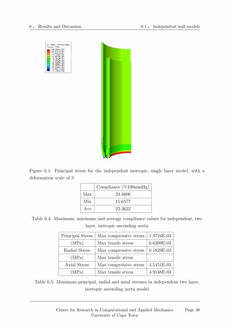
6 � Results and Discussion 6.1 � Independent wall models
Figure 6.1: Principal stress for the independent isotropic, single layer model, with a
deformation scale of 3
Compliance (%100mmHg)
Max 24.4606
Min 15.6577
Ave 22.3622
Table 6.4: Maximum, minimum and average compliance values for independent, two
layer, isotropic ascending aorta
Principal Stress Max compressive stress 1.9724E-03
(MPa) Max tensile stress 6.6309E-03
Radial Stress Max compressive stress 6.1829E-03
(MPa) Max tensile stress –
Axial Stress Max compressive stress 4.5451E-03
(MPa) Max tensile stress 4.9148E-03
Table 6.5: Maximum principal, radial and axial stresses in independent two layer,
isotropic ascending aorta model
Page 48Centre for Research in Computational and Applied MechanicsUniversity of Cape Town

6 � Results and Discussion 6.1 � Independent wall models
Figure 6.2: Principal strain for the independent isotropic, single layer model, with a
deformation scale of 3
Principal Strain Max compressive –
- Max tensile 0.0960
E11 Max compressive 0.1145
- Max tensile –
E22 Max compressive 0.1145
- Max tensile 0.0478
Table 6.6: Maximum principal, radial and axial stresses in independent, two layer,
isotropic ascending aorta model
Page 49Centre for Research in Computational and Applied MechanicsUniversity of Cape Town

6 � Results and Discussion 6.1 � Independent wall models
Figure 6.3: Principal stress for the independent isotropic, two layer model, with a de-
formation scale of 3
Page 50Centre for Research in Computational and Applied MechanicsUniversity of Cape Town

6 � Results and Discussion 6.1 � Independent wall models
Figure 6.4: Principal strain for the independent isotropic, two layer model, with a
deformation scale of 3
Page 51Centre for Research in Computational and Applied MechanicsUniversity of Cape Town

6 � Results and Discussion 6.1 � Independent wall models
6.1.3 Independent two layer, orthotropic model
The values for this model are set out in the Tables 6.7, 6.8 and 6.9, and contour plots
of the principal stresses and strains are displayed in Figures 6.5 and 6.6.
Compliance (%100mmHg)
Max 27.1784
Min 17.1680
Ave 24.8793
Table 6.7: Maximum, minimum and average compliance values for independent, two
layer, orthotropic ascending aorta
Principal Stress Max compressive stress 5.2073E-03
(MPa) Max tensile stress 8.3529E-03
Radial Stress Max compressive stress 6.6637E-03
(MPa) Max tensile stress –
Axial Stress Max compressive stress 5.2078E-03
(MPa) Max tensile stress 6.0144E-03
Table 6.8: Maximum principal, radial and axial stresses in independent two layer,
orthotropic ascending aorta model
Principal Strain Max compressive –
- Max tensile 0.1067
E11 Max compressive 0.1208
- Max tensile –
E22 Max compressive 0.0254
- Max tensile 0.0491
Table 6.9: Maximum principal, radial and axial stresses in independent, two layer,
orthotropic ascending aorta model
6.1.4 Aged aorta model
It can be seen immediately from the visualisation (Figures 6.7, 6.8 and 6.9) of the three
diseased aorta models under a constant pressure load that the results are not accurate.
Therefore this model was not included in a coupled process.
Page 52Centre for Research in Computational and Applied MechanicsUniversity of Cape Town

6 � Results and Discussion 6.1 � Independent wall models
Figure 6.5: Principal stress for the independent orthotropic, two layer model, with a
deformation scale of 3
Page 53Centre for Research in Computational and Applied MechanicsUniversity of Cape Town

6 � Results and Discussion 6.1 � Independent wall models
Figure 6.6: Principal strain for the independent orthotropic, two layer model, with a
deformation scale of 3
Figure 6.7: Resulting geometry of arteriosclerosis with a 0.2mm intima layer
Page 54Centre for Research in Computational and Applied MechanicsUniversity of Cape Town

6 � Results and Discussion 6.1 � Independent wall models
Figure 6.8: Resulting geometry of arteriosclerosis with a 0.4mm intima layer
Figure 6.9: Resulting geometry of arteriosclerosis with a 0.6mm intima layer
Page 55Centre for Research in Computational and Applied MechanicsUniversity of Cape Town

6 � Results and Discussion 6.2 � Independant blood flow models
6.1.5 Discussion of the independent wall models
The data shows a maximum compressive principal stress value existing in the two layer,
orthotropic model, with a value of 5.21× 10⁻³MPa. The tensile value was also highest
in this model, with a value of 8.3529 × 10⁻³MPa. The tensile stress values get higher
with the complexity of the model.
This effect is likely to be due to the different material properties of the layers non-
linearising the elastic properties.
None of the models experienced any tensile stresses or strains in the radial direction,
but this due to the particular loading of the specimen. In the axial direction there was
some tensile stress, which may be due to the “stretching” of the specimen to compensate
for the expansion under the inlet and outlet constraints.
The maximum compliance was greatest in the two layer, orthotropic model and the
differences in maximum and minumum values for all of the models were within 10% of
each other. The lower compliance values are due to the constraints around the aorta
at the inlet, preventing expansion at this point. The minimum values are not entirely
relevant, as the constraints act as a counter-pressure, and thus the applied pressure is
not a sensible value.
6.2 Independant blood flow models
6.2.1 Results of investigation into inlet velocity profile
As discussed in Section 4.6 a relatively flat velocity profile was expected. The investi-
gation yeilded a profile in accordance with this expectation as shown in Figure 6.10.
At the nodes just in from the wall, the velocity magnitude was approximately 4.62×10³m/s, which is 7.84% of the average value.
The velocity magnitude did not reach a peak value on the axis of symmetry, but rather
dipped slightly in the this region. The maximum velocity value occured at a radius of
10.36mm, and was 12.06× 10²m/s. At the centre of the aorta the velocity was equal to
99.15× 10²m/s.
Page 56Centre for Research in Computational and Applied MechanicsUniversity of Cape Town
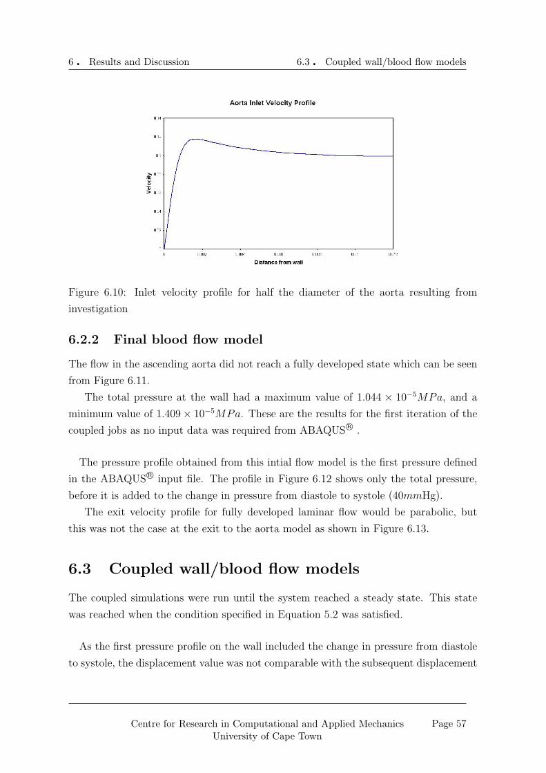
6 � Results and Discussion 6.3 � Coupled wall/blood flow models
Figure 6.10: Inlet velocity profile for half the diameter of the aorta resulting from
investigation
6.2.2 Final blood flow model
The flow in the ascending aorta did not reach a fully developed state which can be seen
from Figure 6.11.
The total pressure at the wall had a maximum value of 1.044 × 10⁻⁵MPa, and a
minimum value of 1.409× 10⁻⁵MPa. These are the results for the first iteration of the
coupled jobs as no input data was required from ABAQUS R© .
The pressure profile obtained from this intial flow model is the first pressure defined
in the ABAQUS R© input file. The profile in Figure 6.12 shows only the total pressure,
before it is added to the change in pressure from diastole to systole (40mmHg).
The exit velocity profile for fully developed laminar flow would be parabolic, but
this was not the case at the exit to the aorta model as shown in Figure 6.13.
6.3 Coupled wall/blood flow models
The coupled simulations were run until the system reached a steady state. This state
was reached when the condition specified in Equation 5.2 was satisfied.
As the first pressure profile on the wall included the change in pressure from diastole
to systole, the displacement value was not comparable with the subsequent displacement
Page 57Centre for Research in Computational and Applied MechanicsUniversity of Cape Town

6 � Results and Discussion 6.3 � Coupled wall/blood flow models
Figure 6.11: Velocity contours resulting from initial flow model
Figure 6.12: Pressure profile output from initial CFD simulation
Figure 6.13: Outlet velocity profile for half the diameter of the ascending aorta
Page 58Centre for Research in Computational and Applied MechanicsUniversity of Cape Town

6 � Results and Discussion 6.3 � Coupled wall/blood flow models
values and was this initial iteration is not shown in the relevant graphs in the following
sections. The same blood flow model was used for all of the wall models. The size of
the displacement of the central boundary node for each iteration was compared with
that for the previous iteration, and the difference in these values is shown in the graphs
displayed for each section.
6.3.1 Coupled single layer, isotropic model
The difference between subsequent displacement sizes of the central boundary node are
shown in Figures 6.14 and 6.15.
Figure 6.14: Graph showing con-
vergence process for radial dis-
placements in the isotropic, single
layer model
Figure 6.15: Graph showing con-
vergence process for axial displace-
ments in the isotropic, single layer
model
The results for this model are shown in the tables below:
Compliance (%/100mmHg)
Max 25.1134
Min 3.5858
Ave 21.6846
Table 6.10: Maximum, minimum and average compliance values for coupled, single
layer, isotropic ascending aorta
6.3.2 Coupled two layer, isotropic model
The difference between subsequent displacement sizes of the central boundary node are
shown in Figures 6.16 and 6.17.
The results for this model are shown in the Tables 6.13, 6.13 and 6.15.
Page 59Centre for Research in Computational and Applied MechanicsUniversity of Cape Town

6 � Results and Discussion 6.3 � Coupled wall/blood flow models
Principal Stress Max compressive stress 1.0700E-03
(MPa) Max tensile stress 1.1886E-02
S11 Max compressive stress 5.2820E-03
(MPa) Max tensile stress 4.9920E-03
S22 Max compressive stress 1.2464E-02
(MPa) Max tensile stress 1.1862E-02
Table 6.11: Maximum principal, radial and axial stresses in coupled single layer,
isotropic ascending aorta model
Principal Strain Max compressive –
- Max tensile 0.1152
E11 Max compressive 0.1076
- Max tensile 0.0903
E22 Max compressive 0.1296
- Max tensile 0.1148
Table 6.12: Maximum principal, radial and axial stresses in coupled, single layer,
isotropic ascending aorta model
Compliance (%/100mmHg)
Max 25.2184
Min 1.3567
Ave 21.6203
Table 6.13: Maximum, minimum and average compliance values for coupled, two layer,
isotropic ascending aorta
Principal Stress Max compressive stress 1.2920E-03
(MPa) Max tensile stress 1.5357E-02
S11 Max compressive stress 5.2830E-03
(MPa) Max tensile stress 4.8740E-03
S22 Max compressive stress 1.0601E-02
(MPa) Max tensile stress 1.5317E-02
Table 6.14: Maximum principal, radial and axial stresses in coupled two layer,
isotropic ascending aorta model
Page 60Centre for Research in Computational and Applied MechanicsUniversity of Cape Town

6 � Results and Discussion 6.3 � Coupled wall/blood flow models
Figure 6.16: Graph showing con-
vergence process for radial dis-
placements for the isotropic, two
layer model
Figure 6.17: Graph showing con-
vergence process for axial displace-
ments for the isotropic, two layer
model
Principal Strain Max compressive –
- Max tensile 0.1315
E11 Max compressive 0.1182
- Max tensile 0.1177
E22 Max compressive 0.1600
- Max tensile 0.1308
Table 6.15: Maximum principal, radial and axial stresses in Coupled, two layer,
isotropic ascending aorta model
6.3.3 Coupled two layer, orthotropic model
The difference between subsequent displacement sizes of the central boundary node are
shown in Figures 6.18 and 6.19.
Figure 6.18: Graph showing con-
vergence process for radial dis-
placements for the orthotropic, two
layer model
Figure 6.19: Graph showing con-
vergence process for axial displace-
ments for the orthotropic, two layer
model
Page 61Centre for Research in Computational and Applied MechanicsUniversity of Cape Town

6 � Results and Discussion 6.3 � Coupled wall/blood flow models
The results for this model are shown in the Tables 6.16, 6.17 and 6.18 and contour
plots of the maximum principal stresses and strains are displayed in Figures 6.20 and
6.21
Compliance (%/100mmHg)
Max 27.9850
Min 2.0297
Ave 24.0727
Table 6.16: Maximum, minimum and average compliance values for coupled, two layer,
orthotropic ascending aorta
Principal Stress Max compressive stress 1.6540E-03
(MPa) Max tensile stress 1.7193E-02
S11 Max compressive stress 5.2750E-03
(MPa) Max tensile stress 4.8510E-03
S22 Max compressive stress 1.1142E-02
(MPa) Max tensile stress 1.7161E-02
Table 6.17: Maximum principal, radial and axial stresses in coupled two layer,
orthotropic ascending aorta model
Principal Strain Max compressive –
- Max tensile 0.1351
E11 Max compressive 0.1251
- Max tensile 0.1199
E22 Max compressive 0.1665
- Max tensile 0.1347
Table 6.18: Maximum principal, radial and axial stresses in coupled, two layer,
orthotropic ascending aorta model
The final flow domain for the orthotropic, two layer model is shown in Figure 6.22
to illustrate the adapted grid as outlined in Chapter 5. Figure 6.3.3 shows the velocity
contours resulting from this grid.
The pressure profile alters due to the different grid geometry as shown in Figure
6.23, which is the final pressure profile applied to the ABAQUS R© model in the coupled
orthotropic, two layer model.
Page 62Centre for Research in Computational and Applied MechanicsUniversity of Cape Town

6 � Results and Discussion 6.3 � Coupled wall/blood flow models
Figure 6.20: Principal stress for the coupled orthotropic, two layer model for the first
iteration, with a deformation scale of 3
Page 63Centre for Research in Computational and Applied MechanicsUniversity of Cape Town

6 � Results and Discussion 6.3 � Coupled wall/blood flow models
Figure 6.21: Principal strain for the coupled orthotropic, two layer model for the first
iteration, with a deformation scale of 3
Figure 6.22: The adapted mesh for the final orthotropic, two layer flow domain
Page 64Centre for Research in Computational and Applied MechanicsUniversity of Cape Town

6 � Results and Discussion 6.3 � Coupled wall/blood flow models
Figure 6.23: Pressure profile reulting from final CFD simulation in the orthotropic, two
layer model
Page 65Centre for Research in Computational and Applied MechanicsUniversity of Cape Town

6 � Results and Discussion 6.4 � Discussion and comparison of results
6.3.4 Discussion of coupled results
As in the independant models the greatest maximum principal stress result occured in
the orthotropic, two layer model, with a value of 1.65 × 10⁻³MPa for the compressive
stress and 1.72 × 10⁻²MPa for the tensile stress. Again the values increased with the
complexity of the model.
As before the maximum compliance value occurred in the orthotropic two layer model,
with a value of 27.99%. The minimum compliance values were all less than 5%, but these
values occurred close to the inlet and may be attributed to the constraints in this region.
6.4 Discussion and comparison of results
6.4.1 Stress and strain values
The maximum compressive principal stress value was 5.2073 × 10⁻³MPa and occured
in the orthotropic, two layer independent model, while the minimum value was 3.1148×10⁻⁴MPa and occurred in the independent isotropic, single layer model. The fact that
these extremes occured in the independent models shows that the pressure profile from
the blood flow may have a smoothing effect on the stresses occurring in the walls. The
pressure drop may also account for lowered stresses in the coupled models.
The maximum principal strain value occured in the coup led orthotropic, two layer
model, with a value of 0.1351MPa. The strain values for the independent models were
all within 0.0107MPa of each other, and those for the coupled models were within
0.0199MPa of each other and all of the strains were tensile.
The principal stresses and strains were generally larger for the coupled models, but
this may be attributed to the fact that a differential pressure added for each iteration,
effectively building on to the initial pressure. Where this is not the case, is likely to
be due to the pressure drop, through the flow domain, lowering the overall value of the
pressure.
Also, the non-linearity of the pressure profile is likely to cause the aorta to deform
non-uniformly. The uneven deformations resulting from this may “pull” the material in
different directions, increasing the tension through the vessel. This may also have been
the cause of the radial tensile stresses and strains occuring in the coupled models in that
as the pressure profile becomes uneven, the load is no longer fully compressive.
Page 66Centre for Research in Computational and Applied MechanicsUniversity of Cape Town

6 � Results and Discussion 6.4 � Discussion and comparison of results
It is apparent that the high stress regions are generally in the constrained sections of
the models. These sections include the inlet constraint, where the vessel has a concen-
trated stress region over the supported inlet region, and the outlet condition, where the
interaction seems to be pulling the aorta, preventing the deformations.
The radial stresses were mainly compressive, which is expected as there is an expansion
in the direction of the force, while the axial stresses are mainly tensile, due to the
stretching of the aorta because of the outlet condition.
6.4.2 Compliance values
The compliance in the models ranged between minimum values of 1.36% and 17.1 7%
,and maximum values of 24.46% and 27.99%. The minimum values were due to the
small displacements in the inlet region, where the constraints prevent them from having
larger values. The fact that there is essentially a pressure opposing the movement makes
this small compliance value irrelevant.
The average compliance values for the coupled jobs differed from those for the inde-
pendent models by 0.67% for the isotropic single layer model, 0.74% for the isotropic
two layer model and 0.81% for the orthotropic two layer model. The average values
for the all of the independent models were higher, but this is due to the low minimum
values. The maximum compliance value for every independent model is lower than that
of its corresponding coupled model, therefore it is safe to say that the effect of the blood
flow on the aorta was to increase the compliance.
The compliance values (both the average and maximum values) are within the range
for physiological values with the two layer, orthotropic model yielding the greatest com-
pliance value of 27.99%, as compared to the lowest maximum value, occuring in the
isotropic, two layer model, of 24.46%.
6.4.3 Mesh refinements
It was important that a finer mesh would not yield substantially different results. There-
fore the initial, independent wall jobs were run with a refined mesh. The difference in
results obtained were unsubstantial and therefore the mesh was not altered.
Page 67Centre for Research in Computational and Applied MechanicsUniversity of Cape Town

Chapter 7
Conclusions and Recommendations
7.1 Consistency of results
The resulting maximum and average compliance values in the investigation of a young
and healthy were all well within the physiological range. The minimum values were lower
than those in physiological data, but this is due to the particular constraints around
these regions (those close to the aorta inlet) and therefore does not negate the relevance
of the other data.
The stress and strain values in the investigation may be seen as verified as they have a
direct relationship with the displacement and pressure values resulting in the compliance.
The range of physiological data is very large, so there is room for very different results to
exist and therefore the data aquired in this investigation should not be seen as conclusive.
The suspicious results yielded in the diseased aortic model should be investigated, as
they are not consistent with the results from the other models. The effects of such drastic
geometrical changes in an ascending aorta on blood flow should also be investigated, in
case of there being a reasonable cause for results of this nature.
7.2 Relevance of investigation
The realistic values obtained as discussed in the previous section and their consistency
with the uncoupled simulations show that the coupling process used was effective.
68

7 � Conclusions and Recommendations 7.3 � Linear elasticity and steady flow
7.3 Linear elasticity and steady flow
The non-linearity of artery walls has a smoothing effect on the pressure waves in the
arterial system. One of the effects of this is the effective pushing of blood onward
through the arteries, releasing strain on the heart. If the blood flow in the models had
been modelled as pulsatile, the linear elastic artery would not have shown any of this
effect. Also, if the artery elasticity were modelled as non-linear, while the blood flow
were transient, the reality of the interaction would again not be fully captured.
7.4 The limitations of axi-symmetric modelling
The axi-symmetric nature of the model was directly associated with the appriximation
of the ascending aorta being a straight cylinder. The irregularity of the aorta geometry
may cause a number of interesting effects on the blood flow that cannot be captured
by an axisymmetric modelling process and an investigation into this would be of great
value.
7.5 Further developments to the artery wall models
A bottom up engineering approach was used in this investigation, and there are many
extensions which could be implemented. The effects of visco-elasticity should be anal-
ysed, possibly starting with a hyper-elastic model to investigate the non-linearity of the
mechanical properties with increased loading.
As previously discussed, the effects of a three dimensional geometry should be included
in subsequent studies.
7.6 Further developments to the blood flow models
The blood flow in this study was not pulsatile. The true nature of blood flow and its
effects on the artery walls requires a fully transient model, especially with regard to the
stresses induced in the artery walls.
Page 69Centre for Research in Computational and Applied MechanicsUniversity of Cape Town

7 � Conclusions and Recommendations7.7 � Further developments to the coupling method
7.7 Further developments to the coupling method
The static nature of the simulations in ABAQUS R© and FLUENT R© forced the superpo-
sition of resulting values, this may have led to a certain amount of error in the results.
A coupling procedure that allows a dynamic analysis process to be carried out would
be of great value here, and the use of an investigation, either using existing software
(for example MpCCI R© ) or the creation of an extended interfacing code (such as that
created for the purpose of this study) is highly recommended.
Page 70Centre for Research in Computational and Applied MechanicsUniversity of Cape Town

References
[1] F.H. Netter. Interactive Atlas of Human Anatomy. Novartis, Summit, USA (NJ),
1998.
[2] Lung National Heart, Blood Institute: Diseases, and conditions index: How
the heart works. http://www.nhlbi.nih.gov/health/dci/Diseases/Hf/HF_
HowHeartWorks.html. last accessed: October 2006.
[3] G.A. Holzapfel. A new constitutive framework for arterial wall mechanics and a
comparative study of material models. Journal of elasticity, 61(8), November 2000.
[4] A. Herrmann. Numerical modelling of cardiovascular prostheses incorporating niti-
nol structure. Master’s thesis, Cardiovascular Research Unit, University of Cape
Town, 2005.
[5] MpCCI Documentation.
[6] Y.C. Fung. Biomechanics: Mechanical properties of living tissues. Springer-Verlag,
New York, 2nd edition, 1993.
[7] Thorsten Koch. Non-linear finite element analyses of the aortic heart valve. Master’s
thesis, Department of Mathematics and Applied Mathematics, University of Cape
Town, September 2004.
[8] Janoske, Silber, Kroger, Stanull, Benderoth, Schmitz-Rixen, Vogl, and Moosdorf.
Fluid-structure interaction in abdominal aortic aneurysms. Journal of Biomechan-
ics, 127(775), 2005.
[9] R.D. Cook. Finite element modelling for stress analysis. John Wiley and Sons,
Inc., 1995.
[10] H.K. Versteeg and W. Malalasekera. An Introduction to Computational Fluid Dy-
namics, the Finite Volume Method. Pearson Prentice Hall, 1995.
71

References References
[11] Robert E. Shadwick. Mechanical design in arteries. The Journal of Experimental
Biology, 202(23):3305–13, 1999.
[12] Karl Perktold and Gerhard Rappitsch. Computer simulation of local blood flow and
vessel mechanics in a compliant carotid artery bifurcation model. J. Biomechanics,
28(7):845–856, 1995.
[13] K. Perktold, R.O. Peter, M. Resch, and G. Langs. Pulsatile non-newtonian flow
characteristics in three-dimensional carotid bifurctaion models: numerical study of
flow phenomena under different bifurcation angle. Journal of Biomedical Engineer-
ing, 13:507–515, 1991.
[14] K. Perktold and G. Rappitsch. Mathematical modelling of local arterial flow and
vessel mechanics. Computational Methods for Fluid-Structure Interaction, 1994.
[15] H.P. Osenberg. Simulation des arteriellen bluflusses- ein allgemeines modell mit
anwendung auf das menschliche hiringefabsystem. ETH-Zurich, 9342.
[16] Feng Gao, Masahiro Watanabe, and Teruo Matsuzawa. Stress analysis in a layered
aortic arch model under pulsatile blood flow. BioMedical Engineering Online, 5(25),
April 2006.
[17] G. Pedrizzetti et al. Pulsatile flow in moderately elastic arteries, its modelling and
effects on elasticity. Comuter Methods in Biomechanics and Biomedical Engineer-
ing, 5(3):219–231, 2002.
[18] Abaqus Theory Manual.
[19] Fluent Theory Manual.
[20] Y. Papaharilaou, D.J. Doorly, and S.J. Sherwin. The influence of out-of-plane
geometry on pulsatile flow within a distal end-to-side anastomosis. J. Biomech,
35:1225–1239, 2002.
[21] J.G Myers, J.A. Moore, M. Ojha, K.W. Johnston, and C.R. Ethier. Factors influ-
encin blood flow patterns in the human right coronary artery. Ann. Biomed. Eng.,
29:109–120, 2001.
[22] B. Berthier, R. Bouzerar, and C. Legallais. Blood flow patterns in an anatomically
realistic coronary vessel: influence of three different reconstruction methods. J.
Biomech, 35:1347–1356, 2002.
Page 72Centre for Research in Computational and Applied MechanicsUniversity of Cape Town

References References
[23] T. Naruse and K. Tanishita. Large curvature effect on pulsatile entrance flow in a
curved tube: model experiment simulating blood flow in aortic arch. J. Biomech
Eng., 118:180–186, 1996.
[24] L. Morris, P. Delassus, A. Callanan, M. Walsh, F. Wallis, P. Grace, and T. Mc-
Gloughlin. 3-d numerical simulation of blood flow through models of the human
aorta. Journal of Biomechanical Engineering, 127:767–774, October 2005.
[25] N. Shahcheragi, H.A. Dwyer, A.Y. Cheer, A.I.Barakat, and T. Rutaganira. Un-
steady and three dimensional simulation of blood flow in the human aortic arch. J.
Biomech Eng., 124:378–387, 2002.
[26] N. Engel. Abdominal aortic aneurysm and low back pain. Dynamic Chiropractic,
14(16), 1996.
[27] W.F. Ganong. Review of Medical Physiology. Lange Medical Publications, 1963.
[28] C.A. Schulze-Bauer, C. Morth, and G.A. Holzapfel. Passive biaxial response of aged
human iliac arteries. Journal of Biomechanical Engineering, 125:395–496, 2003.
[29] Glossary of Terms for the Institute for Non-Newtonian Fluid Mechanics Mechanics
Institute for Non-Newtonian Fluid. http://innfm.swan.ac.uk/innfm/updated/
content/about/glossary. last accessed: October 2006.
[30] Gerhard A. Holzapfel. Determination of material models for arterial walls from
uniaxial extension tests and histological structure. Journal of Theoretical Biology,
May 2005.
[31] W. von Maltzahn, R.G. Warriyar, and W.F. Keitzer. Experimental measurements
of elastic properties of media and adventitia of bovine carotid arteries. Journal of
Biomechanics, 17:839–847, 1984.
[32] University of Cape Town members Cardiovascular Research Unit. Private commu-
nication, 2006.
[33] T. Koch and T. Franz. Review of properties of native human aorta at different
sites. Technical report, Cardiovascular Research Unit, University of Cape Town,
2006.
[34] M.K. Erol, M. Yilmaz, Y. Oztasyonar, S. Sevimli, and H. Senocak. Aortic disten-
sibility is increasing in athletes. Am J Cardiol, 89(8):1002–4, 2002.
Page 73Centre for Research in Computational and Applied MechanicsUniversity of Cape Town

References References
[35] K. Hirata, F. Triposkiadis, E. Sparks, J. Bowen, C.F. Wooley, and H. Boudoulas.
The marfan syndrome, abnormal aortic elastic properties. J Am Coll Cardiol,
18(1):57–63, 1991.
[36] Y.C. Fung. Biomechanics Circulation. Springer, New York, 2nd edition, 1997.
[37] J.D. Hart. Nonparametric Smoothing and Lack-of-Fit Tests. Springer-Verlag New
York Inc, first edition, 1997.
[38] R.M. Nerem, W.A. Seed, and N.B. Wood. An experimental study of the velocity
distribution and transition to turbulence in the aorta. Journal of Fluid Mechanics,
52:137–160, 1972.
[39] W. Nichols and M.F. Rourke. McDonald’s Blood Flow in Arteries. Edward Arnold,
London, fourth edition, 1998.
[40] Fluent help.
[41] R.M. Nerem. Vascular fluid mechanics, the arterial wall, and atherosclerosis. Jour-
nal of Biomechanical Engineering, 114:274–282, 1992.
[42] R.M. Nerem, M.J.A. Rumberger, D.R. Gross, R.L. Hamlin, and G.L.Geiger. Hot-
film anemometry velocity measurements of arterial blood flow in horses. Circ. Res.,
10:301–313, 1974.
[43] H. Falsetti, K.M. Kiser, G.P. Francis, and E.R. Belmore. Sequential velocity devel-
opment in the ascending and descending aorta of the dog. Circ. Res., 21:328–338,
1972.
[44] W.A. Seed and N.B. Wood. Velocity patterns in the aorta. Cardiovasc. Res.,
5:319–330, 1971.
[45] J.F. Douglas, J.M. Gasiorek, and J.A. Swaffield. Fluid Mechanics. Pearson Prentice
Hall, 4th edition, 2001.
Page 74Centre for Research in Computational and Applied MechanicsUniversity of Cape Town