A numerical method for osmotic water flow and solutediffusion with deformable membrane boundaries in two spatial

dimension

Lingxing Yaoa, Yoichiro Morib

aDepartment of Mathematics, Applied Mathematics, and Statistics, Case Western Reserve UniversitybSchool of Mathematics, University of Minnesota

Abstract

Osmotic forces and solute diffusion are increasingly seen as playing a fundamental rolein cell movement. Here, we present a numerical method that allows for studying theinterplay between diffusive, osmotic and mechanical effects. An osmotically active soluteobeys a advection-diffusion equation in a region demarcated by a deformable membrane.The interfacial membrane allows transmembrane water flow which is determined by os-motic and mechanical pressure differences across the membrane. The numerical methodis based on an immersed boundary method for fluid-structure interaction and a Carte-sian grid embedded boundary method for the solute. We demonstrate our numericalalgorithm with the test case of an osmotic engine, a recently proposed mechanism forcell propulsion.

Keywords: Fluid structure interaction, Osmosis, Immersed boundary method,Cartesian grid embedded boundary method, Advection diffusion

1. Introduction

Differences in solute concentration across a semipermeable membrane or interfacegenerates transmembrane osmotic water flow, which is of central importance in dialysisand desalination [1, 2], water absorption in epithelial systems [3, 4], and the swelling/de-swelling of polyelectrolyte gels [5, 6]. The interaction of such flows with membrane andflow mechanics is a little explored area despite its potential significance in science andengineering [7, 8]. Here, we consider a model problem of such an interaction.

Our interest in this problem stems primarily from the problem of cell movement.Much recent evidence suggests that membrane ion channels and aquaporins (water chan-nels), and thus, solute diffusion and osmosis, play an important role in cell movement[9, 10, 11]. To clarify the role of osmosis in cell movement, one needs to understand theinterplay between solute diffusion, osmosis and mechanical forces. Our contribution inthis paper is a step toward building a computational tool to study this interplay.

Email addresses: lxy195@case.edu (Lingxing Yao), ymori@umn.edu (Yoichiro Mori)

Preprint submitted to Elsevier October 10, 2017

In this paper, we present a numerical method for the following model problem intwo spatial dimension. A cell (or a number of cells) is immersed in a surrounding fluidseparated by the cell membrane. The cell membrane is elastic and the fluid flow satisfiesthe Stokes equation. Un-charged solutes diffuse and are advected with the fluid flow,and may pass through the membrane through active and passive mechanisms. To allowfor transmembrane water flow, the membrane has a slip velocity with respect to theunderlying fluid flow. This slip velocity is determined by the jump in the mechanicalas well as the osmotic pressure across the membrane. The problem we consider in thispaper is close to the problems considered in [12, 13, 14, 15, 16]. In [12, 15], the authorconsiders the problem in which the membrane is permeable to water but not to solute(semipermeable membrane). In papers [13, 14] the authors extend the numerical methodin [12] to the case when the membrane may be permeable to both solute and water.In [16], the authors incorporates osmotic forces as as part of a fluid-solute-structureinteraction term. We also mention the recent work in [17], where the authors considerthe well-posedness of a related problem.

We now briefly discuss our numerical method. At each time step, we alternate betweensolving the fluid-structure interaction problem and the solute diffusion problem. For thefluid-structure interaction problem, we use the immersed boundary (IB) method [18].Once the fluid velocity is found, the position of the membrane (immersed boundarypoints) must be updated. As discussed above, there is a slip between the underlyingfluid velocity and the velocity with which the membrane moves. Problems in whichan interface or structure has a slip velocity have been simulated using the IB methodin numerous papers including [19, 20, 21, 22]. The update of the immersed boundarypoints are treated in an explicit fashion in theses papers. In this paper, we employ apartially implicit treatment of this update, which confers better stability properties toour method.

For the solute diffusion problem, we use a Cartesian grid embedded boundary method[23, 24], which allows us to capture the sharp interfacial discontinuity of the solutionconcentration (and its gradient) across the membrane interface. This is similar in spirit[12, 13, 14, 15] where the immersed interface method [25] is used to deal with the discon-tinuity. The major difference and novelty of our method with respect to previous workis that we treat the solute interface conditions implicitly. The (passive) transmembranesolute flux is proportional to the solute difference and is thus a “diffusive” term. Animplicit discretization of the solute boundary condition is crucial for stability especiallywhen the solute permeability coefficient is large; indeed, we have found that, withoutthis implicit treatment, stable computations require prohibitively small time steps. Forthe solute update step, we thus solve a linear system whose unknowns include the con-centration at Cartesian grid points in the bulk and on both faces of the membrane. Thisis in contrast to previous work in which the unknown values are located only in the bulkgrid points. Our method in this sense is analogous to the augmented methods in theimmersed interface literature [25, 26, 27]. This results in a linear system whose structureis more complicated than in [12, 13, 14, 15] where the boundary conditions are treatedexplicitly. This linear system is solved using preconditioned GMRES.

When the boundary moves, some grid points that were on the intracellular (or ex-tracellular) side of the membrane will be on the other side of the membrane at the nexttime step. To solve the (advection) diffusion equation using the method of lines, we mustmodify the time derivative at these freshly cleared locations; simply using the grid value

2

at the previous time step will not work since the solute concentration is discontinuousacross the interface. We employ a new discretization method for this modification whichavoids a complicated extrapolation procedure.

We test our numerical method using a model problem inspired by the recent ex-perimental results in [28]. In [28], the authors present experimental results in which acancer cell confined to a one-dimensional geometry can move even when its cytoskeletaland motor machinery is disrupted by pharmacological means. The authors suggest thatthis cellular movement is due to osmotic pressure differences, which the cell generatesby pumping solute in at one end of the cell and pumping solute out of the other end.We also point out that this osmotic engine mechanism can be thought of as a version ofosmophoresis [29, 30], in which a vesicle with a semi-permeable membrane moves whensubjected to a externally imposed concentration gradient. The osmotic engine mecha-nism suggested in [28], then, can be seen as osmophoresis with a concentration gradientgenerated by the cell itself. In this paper, we shall test whether such an osmotic enginemechanism can propel the cell forward in a two-dimensional setting using biophysicallyrealistic parameter values, and study the interplay between shape changes, solute diffu-sivity and osmotic forces. Our simulations show that the osmotic engine mechanism is apotentially feasible mechanism of cell propulsion in the 2D setting. We also mention re-lated work in [31, 32, 33], where the authors consider a colloidal particle being propelledby an osmotic mechanism. There, in contrast to our model simulations, a concentrationgradient generated by a chemical reaction provides the driving force for osmotic fluidflow. A variant of this mechanism is also considered in [34, 35].

The outline of our paper is as follows. In Section 2, we define our model problem.In Section 3, we give a detailed description of the numerical algorithm. In Section 4,we present simulations using our numerical method. We first present an example inSection 4.1, in which the solute diffusion component of our method is tested. In Section4.2, we test our numerical method using the osmotic engine model discussed above,which couples solute diffusion with membrane mechanics and fluid flow. In all of thesewe perform convergence studies to confirm the expected convergence rate. Finally, inSection 4.3, we perform further parametric studies on the osmotic engine model.

2. Setup

Consider a rectangular domain Ω ⊂ R2 and one or multiple smooth closed surfacesdenoted by Γ ⊂ Ω. This closed surface divides Ω into two domains. Let Ωi ⊂ Ω bethe region bounded by Γ, and let Ωe = Ω\(Ωi ∪ Γ). The region Ωi the intracellularregion and Ωe is the extracellular region. The equations to follow are written in suitabledimensionless form.

We begin by writing down the equations of chemical concentration c. At any pointin Ωi or Ωe

∂c

∂t+∇ · (uc) = ∇ · (D∇c) (1)

where D is the diffusion coefficient and u is the fluid velocity field.Let us now consider the interfacial boundary conditions on the membrane Γ. Since we

want to account for osmotic water flow, the membrane Γ will deform in time. Sometimes,we shall use the notation Γt to make this time dependence explicit. Let Γref be the resting

3

Ωi

Ωe

Γ

n

ΩiΓ

Figure 1: Diagram of the computational domain and flexible membrane.

or reference configuration of Γ. The membrane will then be a smooth deformation of thisreference surface. We may take a coordinate system s on Γref, which would serve as amaterial coordinate for Γt. The trajectory of a point that corresponds to s = s0 is givenby X(s0, t) ∈ Ω. For fixed t, X(·, t) gives us the shape of the membrane Γt.

Consider a point x = X(s, t) on the membrane. Let n be the outward unit normal onΓ at this point. The boundary conditions satisfied on the intracellular and extracellularfaces of the membrane are given by:

(uc−D∇c) · n = c∂X

∂t· n+ jc + jp on Γi or Γe. (2)

The expression “on Γi,e” indicates that the quantities are to be evaluated on the intra-cellular and extracellular faces of Γ respectively. Equation (2) is just a statement ofconservation of ions at the moving membrane. The sum jc + jp is the transmembranechemical flux. Flux going from Ωi to Ωe is taken to be positive. The flux is divided intothe passive channel flux jc and the active pump flux jp. For jc, we let:

jc = kc [c] , kc = kc

∣∣∣∣∂X∂s∣∣∣∣−1

, (3)

where kc is a positive constant. The Jacobian factor accounts reflects the view thatthe chemicals pass through the membrane through channels, whose density transformsinversely with extension of the membrane. The solute thus flows from where the concen-tration is high to low. For the active flux jp we set:

jp = kpH(s, ci, ce), kp = kp(s)

∣∣∣∣∂X∂s∣∣∣∣−1

,

H(s, ci, ce) =

ci if kp(s) ≥ 0,

ce if kp(s) < 0,

(4)

where ci,e are the values of the concentration at Γi,e respectively. When kp ≥ 0, themembrane pump actively pumps solute out of the cell and the flux is dependent on ci,and vice versa when kp < 0. The Jacobian factor is present for the same reason as for(3).

4

We now discuss force balance. Consider the equations of fluid flow. The flow field usatisfies the Stokes equation in Ωi,e:

0 = ∇ · Σm(u, p), ∇ · u = 0,Σm(u, p) = ν(∇u+ (∇u)T )− pI = 2ν∇Su− pI (5)

where ν > 0 is the dynamic viscosity, I is the 2 × 2 identity matrix and (∇u)T is thetranspose of ∇u, and p is the pressure. We have introduced the notation ∇S to denotethe symmetric part of the velocity gradient. Σm is just the Stokes stress tensor.

We now turn to boundary conditions at the cell membrane Γ. Take a point x =X(s, t) on the boundary Γ, and let n be the unit outward normal on Γ at this point.First, by force balance, we have:

[Σm(u, p)n] = Fmem. (6)

Here, Fmem is the elastic force per unit area of membrane and [·] denotes the jump inthe enclosed quantity across the membrane (evaluation on Γi minus evaluation on Γe).

For Fmem, we take the constitutive law:

Fmem = Fmem

∣∣∣∣∂X∂s∣∣∣∣−1

, Fmem = Felas + Fbend,

Felas = kelas∂

∂s

((∣∣∣∣∂X∂s∣∣∣∣− `) τ) , τ =

∂X

∂s

∣∣∣∣∂X∂s∣∣∣∣−1

,

Fbend = −kbend∂4X

∂s4,

(7)

where kelas > 0 is the elasticity constant, ` is the resting length and kbend > 0 is thebending stiffness.

In addition to the force balance condition (6), we need a continuity condition on theinterface Γ. The velocity field is assumed continuous across Γ:

[u] = 0. (8)

Since we are allowing for osmotic water flow, we have a slip between the movement ofthe membrane and the flow field. At a point x = X(θ, t) on the boundary Γ we have:

u− ∂X

∂t= jwn (9)

where jw is water flux through the membrane. We are thus assuming that water flowis always normal to the membrane and that there is no slip between the fluid and themembrane in the direction tangent to the membrane. Given that n is the outwardnormal, jw is positive when water is flowing out of the cell. We let:

jw = kw[ψ], ψ = −RTc− n · ((Σm(u, p))n), (10)

where R is gas constant and T is absolute temperature. Transmembrane water flowis thus driven by the difference in mechanical force ([n · ((Σm(u, p))n)]) as well as thedifference in osmotic pressure ([c]). Given (6), we may also set :

jw = −kw

(RT [c] + Fmem · n

). (11)

5

On the outer boundary of the rectangular region Ω, we set periodic boundary con-ditions in the horizontal x direction for both the concentration c and the velocity fieldu. In the vertical y direction, we set u = 0 and no-flux boundary conditions for theconcentration c.

We point out that the above equations are thermodynamically consistent in the sensethat it satisfies the following free energy identity [36]. Now, suppose c,u, p and X aresmooth functions that satisfy the equations and boundary conditions just described.Then, the following free energy identity holds:

d

dt(Ebulk + Emem) = −I − J,

Ebulk =

∫Ωi∪Ωe

ωdx, ω = RT (c ln c− c),

Emem =

∫Γref

(kelas

(∣∣∣∣∂X∂s∣∣∣∣− `)2

+ kbend

∣∣∣∣∂2X

∂s2

∣∣∣∣2)ds,

I =

∫Ωi∪Ωe

(2ν |∇Su|2 +

D

RTc |∇µ|2

)dx, µ = RT ln c,

J =

∫Γ

([ψ]jw + [µ](jc + jp)) dmΓ, dmΓ =

∣∣∣∣∂X∂s∣∣∣∣ ds.

(12)

Here, |∇Su| is the Frobenius norm of the 2×2 symmetric rate of deformation matrix∇Su.The derivation of this identity follows from a standard integration by parts argument [36],and is given in the Appendix A for convenience of the reader. Note that I ≥ 0 and Jis non-negative if jp is 0. Thus, in the absence of an active pump flux, the free energyis monotone decreasing, in concordance with the second law of thermodynamics. Theabove energy relation, in particular, shows that the only external free energy input tothe system is through active ionic pumps. An interesting aspect of the osmotic enginemechanism we examine in this paper is that this purely chemical free energy input isturned into directional movement.

It will be convenient to rewrite the fluid equations in the following form. Equations(5), (6) and (8) can be written together as:

0 = ν∆u−∇p+ f , ∇ · u = 0, (13)

f(x, t) =

∫Γref

Fmem(X)δ(x−X(s, t))ds, (14)

where δ is the two-dimensional Dirac delta function, and the above equations are to beunderstood in the sense of distributions. The immersed boundary (IB) method, which wewill use for the discretization of the fluid equations, makes use of the above reformulation.

3. Numerical algorithm

We consider a square computational domain Ω = [0, L]× [0, L] and lay a fixed Carte-sian grid with vertices at (xi, yj), xi = i4x, i = 0, . . . , N , yj = j4y, j = 0, . . . , N , andcell centers (xi+ 1

2, yj+ 1

2). In each computational cell, chemical concentration c and fluid

pressure p are defined at the cell center, and the velocity components (u, v) = u are6

arranged at vertical and horizontal edges of the cells respectively, following the MAC(marker and cell) grid arrangement.

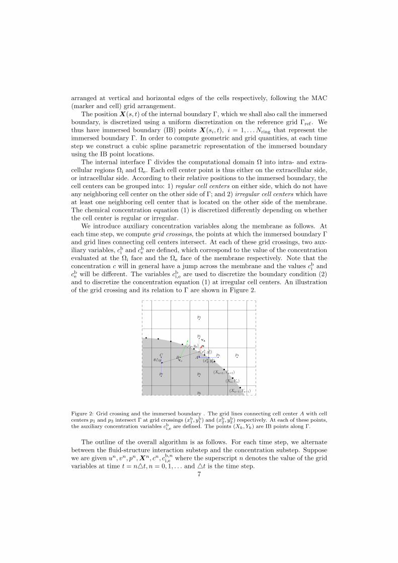
The positionX(s, t) of the internal boundary Γ, which we shall also call the immersedboundary, is discretized using a uniform discretization on the reference grid Γref . Wethus have immersed boundary (IB) points X(si, t), i = 1, . . . Nring that represent theimmersed boundary Γ. In order to compute geometric and grid quantities, at each timestep we construct a cubic spline parametric representation of the immersed boundaryusing the IB point locations.

The internal interface Γ divides the computational domain Ω into intra- and extra-cellular regions Ωi and Ωe. Each cell center point is thus either on the extracellular side,or intracellular side. According to their relative positions to the immersed boundary, thecell centers can be grouped into: 1) regular cell centers on either side, which do not haveany neighboring cell center on the other side of Γ; and 2) irregular cell centers which haveat least one neighboring cell center that is located on the other side of the membrane.The chemical concentration equation (1) is discretized differently depending on whetherthe cell center is regular or irregular.

We introduce auxiliary concentration variables along the membrane as follows. Ateach time step, we compute grid crossings, the points at which the immersed boundary Γand grid lines connecting cell centers intersect. At each of these grid crossings, two aux-iliary variables, cbi and cbe are defined, which correspond to the value of the concentrationevaluated at the Ωi face and the Ωe face of the membrane respectively. Note that theconcentration c will in general have a jump across the membrane and the values cbi andcbe will be different. The variables cbi,e are used to discretize the boundary condition (2)and to discretize the concentration equation (1) at irregular cell centers. An illustrationof the grid crossing and its relation to Γ are shown in Figure 2.

(Xn+1, Yn+1)

(Xn, Yn)

(Xn−1, Yn−1)

(xp, yp)

Bvo

AC

p2

p7

p1va

p6

p3

p5

p4(xb1, y

b1)

n

θ4y (xb2, yb2)

Figure 2: Grid crossing and the immersed boundary . The grid lines connecting cell center A with cellcenters p1 and p3 intersect Γ at grid crossings (xb1 , y

b1 ) and (xb2 , y

b2 ) respectively. At each of these points,

the auxiliary concentration variables cbi,e are defined. The points (Xk, Yk) are IB points along Γ.

The outline of the overall algorithm is as follows. For each time step, we alternatebetween the fluid-structure interaction substep and the concentration substep. Supposewe are given un, vn, pn,Xn, cn, cb,ni,e where the superscript n denotes the value of the gridvariables at time t = n4t, n = 0, 1, . . . and 4t is the time step.

7

Substep 1 Given un, vn, pn and Xn, use the IB method to compute un+1, vn+1 andpn+1 with a discretization of (13), (14) and (7). Computations of (14) and (7)

is performed using Xn. Once this is found, use Xn, cb,ni,e as well as the newly

found un+1, vn+1 to discretize (9) and (11) to obtain the new IB locations Xn+1.Equation (11) requires concentration values at IB locations, which we denote by

cIB,ni,e . This is obtained by interpolating the concentration values cb,ni,e defined atgrid crossings.

Substep 2 Given our new IB point locations Xn+1 and the fluid velocity (un+1, vn+1),solve moving boundary advection diffusion problem for the concentration cn+1 andcb,n+1i,e . At irregular cell centers discretization of equations (1) requires care. This

is especially the case for freshly cleared points, which are computational cell centersthat were located in Ωi in the previous time step but are now in Ωe or vice versa.Boundary conditions (2) are enforced at grid crossing with the help of the auxiliary

concentration variables cbi,e. A linear system for cn+1 and cb,n+1i,e is obtained and

solved using an iterative method.

We now discuss each computational substep in detail.

3.1. Fluid-structure interaction substep

3.1.1. IB method for fluid velocity

Consider the Stokes equation (5) for fluid velocity u and pressure p:

0 = ν∆u−∇p+ f , ∇ · u = 0. (15)

We use immersed boundary method to discretize it. We arrange all variables in a MACgrid, in which the pressure p is defined at cell centers and the velocity field u is defined atthe horizontal (u) and vertical (v) cell faces. Define the following differencing operatorsfor any grid function w, where wnα,β denotes the value of w at (x, y) = (αh, βh) at timet = n4t:

D±x wα,β = ±wα±1,β − wα,βh

, D±y wα,β = ±wα,β±1 − wα,βh

,

Lwα,β = D+x D−x wα,β +D+

y D−y wα,β

=wα+1,β + wα,β+1 + wα−1,β + wα,β−1 − 4wα,β

h2,

(16)

Let u = (u, v), and f = (f, g), equation (15) is then

D−x pn+1i+ 1

2 ,j+12

= νLun+1i,j+ 1

2

+ fni,j+ 12,

D−y pn+1i+ 1

2 ,j+12

= νLvn+1i+ 1

2 ,j+ gni+ 1

2 ,j,

0 = D−x un+1i+1,j+ 1

2

+D−y vn+1i+ 1

2 ,j+1.

(17)

As we assume periodic boundary condition for u and p on the left and right edge of thecomputational domain, and homogeneous Dirichlet boundary condition for u on the topand bottom edges, we can solve (u, v) and p from linear system (17) by using FFT along

8

x direction, which will result in block diagonal linear system to solve at each xi, and canbe solved efficiently using a direct solver.

We turn to the determination of the body forces f = (f, g). Let Fmem = (Fx, Fy) andthe IB point positions X = (X,Y ). For a quantity W defined on the immersed boundarygrid parametrized by s, we let Wk denote the value of W at point s = sk = k4s, where4s is the grid spacing in s. Equation (14) for f = (f, g) are discretized as follows

fni,j+ 12

=

Nring∑k=1

Fnx,kδh(xi −Xnk )δh(yj+ 1

2− Y nk )4s

gni+ 12 ,j

=

Nring∑k=1

Fny,kδh(xi+ 12−Xn

k )δh(yj − Y nk )4s(18)

where δh(r) is a regularized discrete delta function. In this paper, we use the followingdiscrete delta function:

δh(r) =1

hφ( rh

),

φ(r) =

18 (3− 2 |r|+

√1 + 4 |r| − 4r2) |r| ≤ 1,

18 (5− 2 |r| −

√−7 + 12 |r| − 4r2) 1 < |r| ≤ 2,

0 2 < |r| .

(19)

The rationale for this particular choice of regularization is discussed in [18]. To computethe membrane force Fmem let us first introduce the following differencing operators actingon functions W defined on the IB grid:

D±s Wk = ±Wk±1 −Wk

4s , LsWk = D+s D−s Wk. (20)

Using these operators, we discretize (14) as follows:

F nmem,k = kelasD+s

((1− `

∣∣D−s Xnk

∣∣−1)D−s Xn

k

)− kbendLsLsXn

k , (21)

where the differencing operators above act component-wise.Thus, given the IB point locations Xn, the membrane forces Fmem is computed using

(21), which is then used to compute fn with the regularized discrete delta functions asin (18). This body force fn is then fed into equation (17), which is solved to produceun+1 and pn+1.

9

3.1.2. Semi-implicit update of IB locations

We turn to the update of the IB point locations. Combining (9) and (11), we employ

the following discretization (for any grid function w, we have D−t wn = wn−wn−1

4t ):

D−t Xn+1k = Un+1

k − jnw, jnw = −kw

([cIB,nk

]+ F n+1

mem,k · nn), Uk = (Uk, Vk),

F n+1mem,k = F n+1

mem,k

1

2

(∣∣D+s X

n∣∣−1

+∣∣D−s Xn

∣∣−1),

Unk =∑i,j

uni,j+ 12δh(xi −Xn

k )δh(yj+ 12− Y nk )h2,

V nk =∑i,j

vni+ 12 ,jδh(xi+ 1

2−Xn

k )δh(yj − Y nk )h2,

(22)

where F n+1mem,k is specified as in (21). The values cIB,ni,e,k are the intracellular and extra-

cellular concentrations at the IB point k at time n4t, and is evaluated by interpolating

the membrane concentration values at grid crossings cb,ni,e . The jump[cIB,nk

]is equal to

cIB,ni,k − cIB,ne,k . In the right hand side of the first equation, all terms except for Fmem,k are

known quantities. This is thus a nonlinear equation for Xn+1, which is solved using aNewton iteration. We have found that the implicit treatment of Fmem,k lead to betterstability properties.

3.2. Concentration Substep

We turn to the update of the chemicals. The strategy used here in updating chemicalvariables is similar to many Cartesian grid embedded boundary methods (see like [24,23, 37] and many others), which use interpolations to set up locally smooth functionsfor constructing stencils on the Cartesian grids. Our construction of stencils at regularand irregular cell centers and the inclusion of auxiliary variables at grid crossings isinspired by the work in [24]. The most important feature of the concentration substepis that the concentration boundary conditions (2) are treated implicitly, so that theunknown concentrations are located at Cartesian grid points and the grid crossings. Asdiscussed earlier, this has proved crucial for stable computations. Another new featureof our discretization strategy is the treatment of the time derivative in freshly clearedcomputational cell centers, i.e., the cell centers that change sides between time steps.

3.2.1. Regular cell centers

Recall that cell centers can are classified into regular cell centers and irregular cellcenters. The regular cell centers have no neighboring grid cell centers on the other sideof the membrane Γn+1, the immersed boundary defined by the IB point locations Xn+1.

At any regular Cartesian cell center, we use a standard implicit Euler discretizationof the (1):

D−t cn+1i+ 1

2 ,j+12

+D−x(un+1i+1,j+ 1

2

A+x c

n+1i+ 1

2 j+12

)+D−y

(vn+1i+ 1

2 ,j+1A+y c

n+1i+ 1

2 j+12

)=DLcn+1

i+ 12 ,j+

12

,(23)

10

where, for any quantity w on the Cartesian grid,

A+xwα,β =

1

2(wα+1,β + wα,β) , A+

y wα,β =1

2(wα,β+1 + wα,β) , (24)

where α, β are integer or half integer. Note here that the velocity field (un+1, vn+1) havebeen determined at the immersed boundary substep.

At irregular cell centers, the above spatial discretization cannot be performed as is,since some of the concentration variables at neighboring cell centers represent concentra-tions at the other side of the membrane. It may also be the case that the cell center ofinterest was freshly cleared. That is to say, the cell center may have been on the Ωi sideof Γn (the immersed boundary position at the n-th time step) whereas it is on the Ωe

side of Γn+1, or vice versa. In this case, the discretization of the time derivative mustalso be modified. We discuss these two modifications in turn.

3.2.2. Stencil at irregular cell centers

For chemicals at irregular cell centers, we use (23) but with the following modifica-tions. Suppose we try to update the chemical cn+1

A defined at cell center A (containedin Ωi) in Figure 2 using (23). The difference operators require chemical concentrationvariables at p1 and p3 . We obtain an expression for the concentration at these two points(called ghost cells) using an extrapolation procedure using concentration variables at thecell centers and grid crossings in Ωi (where point A is located).

The extrapolation scheme for ghost cell chemicals is adopted from [24]. At point p1,in Figure 2, we use

cp1 =2(1− θ)

2 + θcp6 −

3(1− θ)1 + θ

cp5 +6

(1 + θ)(2 + θ)cbi , (25)

where θ is the ratio of distance from the grid crossing (xb1 , y

b1 ) to A and distance from p1 to

A (grid spacing in the y direction), cp6 and cp5 are chemicals at p6 and p5 respectively, andcbi is the auxiliary intracellular chemical concentration defined at grid crossing (xb

1 , yb1 ).

A similar procedure is performed in the x direction to obtain an extrapolation formulaat point p3.

Equation (25) uses two grid point locations p5 and p6, and in exceptional cases de-pending on the geometry of Γ relative to the Cartesian grid, two such grid points maynot be available. When only one such point is available, we use the formula:

cp1 =−(1− θ)

1 + θcp5 +

2

(1 + θ)cbi . (26)

In the extreme case when no such grid locations are available, we set cp1 = cbi . The useof these lower order extrapolation procedures (as opposed to (25)) will in general lead toorder 1 consistency errors at these grid points. However, the points at which such errorsare committed remains a small fraction of cell centers (the proportion should becomesmaller with finer grid spacing), and thus does not affect the order of convergence, as isdocumented in [24] and demonstrated below.

These extrapolation formulae are substituted into the corresponding terms in (23)to produce the spatial stencil at the irregular cell centers. The stencil at the irregularstencils, therefore, depend not only on concentration values at cell centers but also atgrid crossings cbi or cbe .

11

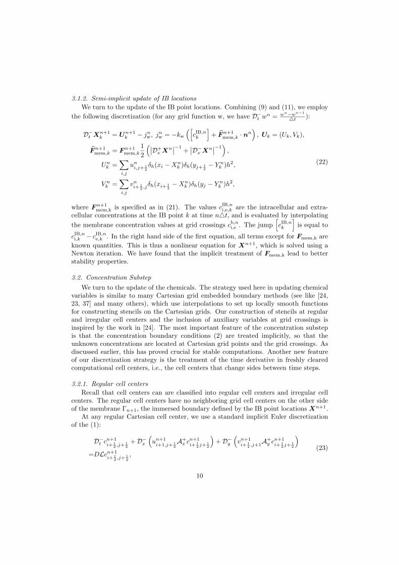
3.2.3. Time discretization at freshly cleared cell

At a freshly cleared cell we must modify the time discretization. Such modificationsare discussed in [23, 38]. Here, we propose new procedure which is simple to implementwith good stability properties.

pFtn+1

tn

py

pxF

p1

p2

Figure 3: Treatment of freshly cleared grid

Consider the point F in Figure 3. It is a freshly cleared point that was in Ωi at timet = n4t but is in Ωe at t = (n+ 1)4t. In evaluating the time differencing term in (23)at this point, cnF has to be available. Since point F was not in Ωe at time level n, cnF isnot available. A standard way to obtain this value is to extrapolate the t = n4t levelchemicals at neighbor cell centers, at p1 and p2, say, on the intracellular side, to F .This extrapolation could lead to large numerical errors especially in extreme geometricsituations. Here we propose a new scheme for the discretization of the time derivative.

First we find the point pF = (x∗F , y∗F ) ∈ Γn that is closest to the point F = (xF , yF ).

The chemical concentration at point pF at time t = n4t (on the extracellular side, whichwe call cne,pF ) may be obtained by interpolating the chemical concentration values at grid

crossings cb,ne at time t = n4t. A (seemingly) reasonable approximation to the partialtime derivative at point F would be:

cn+1F − cne,pF4t . (27)

The above expression, however, will not be a consistent discretization because this differ-encing corresponds to an “advective” derivative. The velocity of this advection is givenby:

(uF , vF ) =

(xF − x∗F4t ,

yF − y∗F4t

). (28)

Therefore, (27) must be corrected to remove the advective component resulting from theabove velocity. The following is thus a consistent discretization of the time derivative ofconcentration cF at point F :

∂cF∂t

∣∣∣∣t=n4t

≈ cn+1F − cne,pF4t − uFD0

xcn+1F − vFD0

ycn+1F . (29)

where

D0x,yw =

1

2

(D+x,yw +D−x,yw

). (30)

12

At freshly cleared points, expression (29) is used in place of the D−t c term in (23). Theabove spatial differencing in many cases involves ghost cell locations. In such cases,extrapolation formulae discussed in Section 3.2.2 are used.

3.2.4. Enforcing chemical boundary condition with auxiliary variables

The chemical boundary conditions (2) are enforced along the membrane Γ, with thehelp of the auxiliary chemicals defined at grid crossings on both sides of the interface.We first rewrite boundary condition (2) using (11), (3) and (4):

jwc−D∇c · n = kc[c] + kpH(s, ci, ce). (31)

Let us consider grid crossing (xb1 , y

b1 ) as in Figure 2. The above boundary condition is

satisfied on both sides of the membrane. We consider the Ωi side of the membrane. Ourdiscretization of (31) is:

jnwcni −DN (cb,n+1

i , cn+1) = kc[cb,n+1] + kpH(s, cni , cne ). (32)

The diffusive flux term and the passive membrane flux term are treated implicitly attime t = (n + 1)4t. This implicit treatment of the boundary condition is the key tostable computations. Our computational experience indicates that an explicit treatmentof these terms leads to persistent spurious oscillations of the chemical concentrations nearthe interfacial boundary. The other terms are evaluated at explicitly, but we point outthat these values are not available at the grid crossings; the above equations are definedon the grid crossings at t = (n + 1)4t but grid crossings change with every time step.We compute these terms in the following fashion. We take jnw and cn defined at IB points(see equation (22), Section 3.1.2) assign these values to the corresponding IB points attime t = (n+ 1)4t. Then, we interpolate these values to the grid crossing locations.

We now discuss the discretization of the normal derivative (the N term in (32)). Ourprocedure follows [24]. Taking intracellular side of the grid crossing at (xb1, y

b1) in Figure

2, the treatment is illustrated as follows.The unit normal direction n along Γ can be decomposed into two directions: along

grid line va (from point p1 to A); and off grid line vo (from boundary point (xb1, yb1)

through grid point B and stop on grid line between C and p7). We thus have n =aovo+aava. With these two directions, the normal derivative ∇cbi ·n can be decomposedas a linear combination of directional derivatives along the vo and va directions:

∇cbi · n = ao∇cbi · vo + aa∇cbi · va

=ao||vo||∂cbi

∂(vo/||vo||)+ aa||va||

∂cbi∂(va/||va||)

.(33)

So along vo and va, we need to approximate the partial derivatives, using chemicals atcell centers and the auxiliary variables at grid crossings. If a first order approximationis used, we will have

∇cbi · n ≈ ao(cB − cbi ) + aa(cp5 − cbi ), (34)

where cB is the chemical at point B, and cbi is auxiliary chemical at the grid crossing onintracellular side. The direction vectors are given by

vo = (xB − xb1, yB − yb1), va = (xp5 − xb1, yp5 − yb1). (35)13

In choosing the cell centers used for this process, we avoid using cell centers that aredirectly adjacent to the grid crossing. Otherwise, vo or va can be arbitrarily small inlength, and the coefficient ao and aa can become arbitrarily large thus leading to possiblenumerical instabilities.

We use higher order approximations if more cell centers are available. For example ifinstead of just using point B for the off grid line direction, we may use point B, C, andp7

∂cbi∂(vo/||vo||)

≈ − 3

2||vo||cbi +

2

||vo||cB −

1

2||vo||[(1− θ)cC + θcp7 ], (36)

and if we use the grid crossing, point p5 and p6, we have

∂cbi∂(va/||va||)

≈ − 1 + θ

(2 + θ)4y cp6 +2 + θ

(1 + θ)4y cp5 −3 + 2θ

(1 + θ)(2 + θ)4y cbi . (37)

The θ here in (37) and (36) is the same as in (25).

3.2.5. Linear Solver

The resulting linear equations have, as unknowns, the concentrations at the cell cen-ters as well as the intracellular and extracellular concentrations at grid-crossings. Thelinear equation is non-symmetric, and we use GMRES with Jacobi preconditioning tosolve this system.

4. Test cases and numerical convergence study

To validate our numerical scheme for simulating chemical advection-diffusion in amoving domain, and the coupling of chemical osmosis effects and fluid structure inter-actions, we design several numerical test cases as follows. We will first test the chemicalmodule only, and then the coupling with fluid flow. In all the examples discussed, pa-rameters are dimensionless.

4.1. Chemical evolution with prescribed cell motion and background flow

We assume that the computational domain, the [0, 1] × [0, 1] unit square, is filledwith an incompressible viscous fluid, and there is a cell with initial configuration r(s)immersed in the domain,

r(s) = 〈0.5 + 0.25 cos s, 0.5 + 0.25 sin s〉. (38)

To verify the accuracy of chemical update module, we consider the situation in whichthe flow field and the immersed boundary locations are prescribed. The update of chem-icals in the whole domain is done with prescribed analytical background fluid velocity uand cell motion dX/dt, as follows:

u = 〈u(x, y), v(x, y)〉 = 〈14− (y − 1

2)2, 0〉; (39)

dX

dt= 〈(1

4− (y − 1

2)2)− 1

2cos t, 0〉. (40)

14

The prescribed background velocity (39) and cell motion (40) will be used in the chemicalboundary condition (2), and (39) in evaluating advection term in the chemical diffusionadvection equation (1). In the chemical boundary condition (2), we allow passive chemicalflux jc through the membrane with constant rate kc = 4 in (3). We set the chemicalpump strength to be kp(s) = 0.1 in (4), so chemicals will be actively moved from theintracellular space to the extracellular space.

To run the chemical module, the diffusion coefficient is set to D = 0.2, and initialchemical field is given by

c(x, y, 0) = 0.5(1.25 + sin(2π(x− 0.5)))(1 + sin(2π(y − 0.25))). (41)

Boundary conditions for the chemicals at the top and bottom of the domain are Dirichletand set to 0, while the left and right edges will have periodic boundary conditions.

In this test case, the cell initially given in (38) is marked by a series Lagrangianmarker points Xi = r(si), and si = (i − 1)2π/Nring, i = 1, . . . , Nring. The velocityof these marker points is prescribed in (40). We should note that here the chemicalboundary condition (2) is implemented without using the water flux term jw, since it isnot available due to the problem set up. The difference in background velocity u andprescribed cell motion is used instead.

0

0.2

0.4

0.6

0.8

1

0 0.2 0.4 0.6 0.8 1

t=0.00t=0.50t=1.00t=1.50t=2.00t=2.25

Figure 4: Test case 1. Cell snapshots with its movement prescribed.

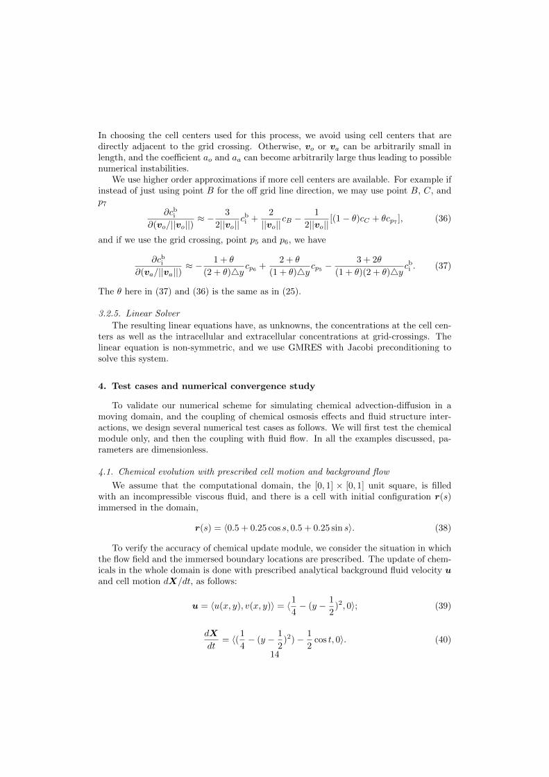
Snapshots of the moving cell are plotted in Figure 4. We can see that the cell movesagainst the background flow to the left first and then to the right, due to the prescribedcell motion. In Figure 5 and 6, snapshots of chemical field with cell locations at those timestamps shown in Figure 4 are plotted using results on a 128× 128 grid with Nring = 320.

In Table 1, we list the convergence rates. To obtain these rates, we use ratios ofdifferences of computed solutions. Set:

ε4x,4t = c4x,4t − Ic4x/2,4t/2, (42)

where subscript 4x,4t indicates levels of space and time spacing, and I is the in-terpolation operator to the coarser grid. We refine 4s proportionally to 4x, i.e., thenumber of immersed boundary marker points is doubled as the Eulerian grid spacing ishalved. The error ratio is computed by:

rp(4x,4t) = ‖ε4x,4t‖p/‖ε4x/2,4t/2‖p (43)15

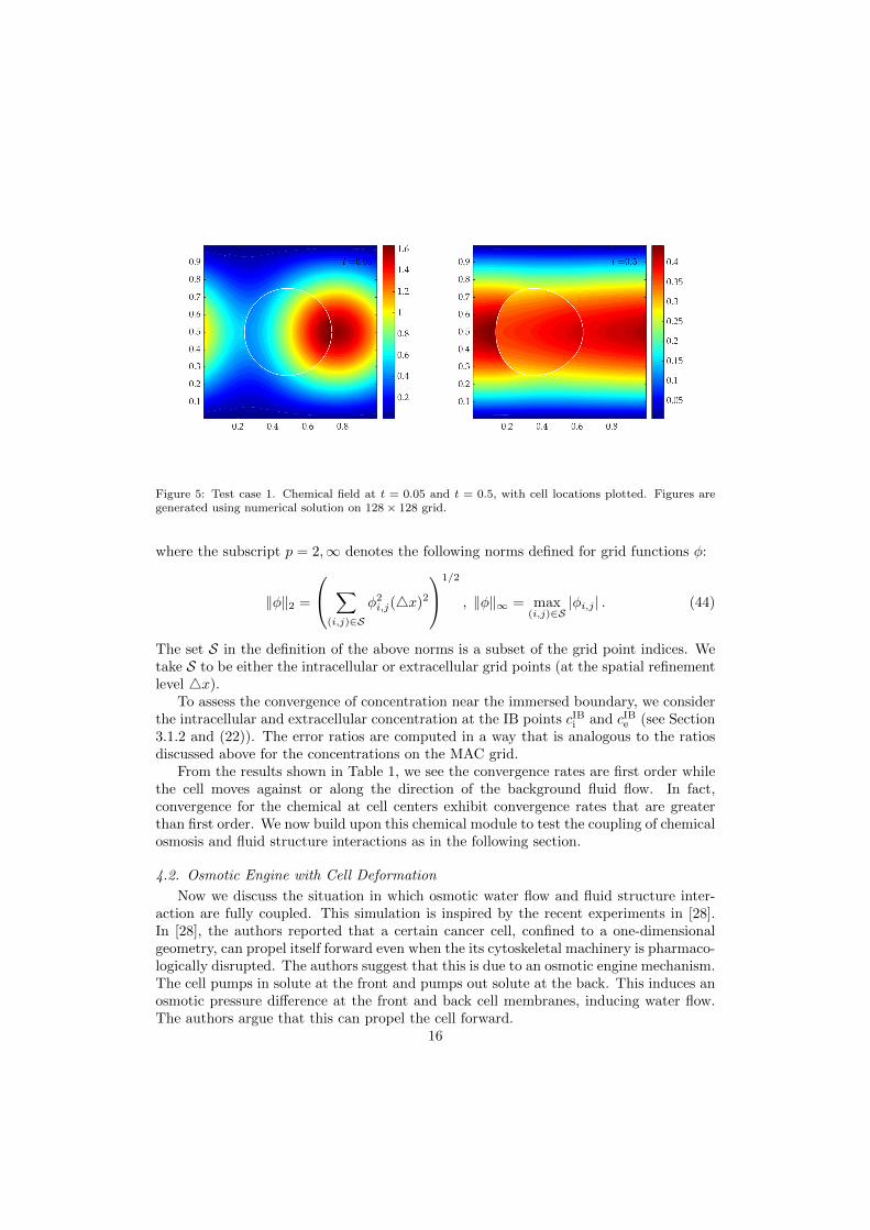
Figure 5: Test case 1. Chemical field at t = 0.05 and t = 0.5, with cell locations plotted. Figures aregenerated using numerical solution on 128× 128 grid.

where the subscript p = 2,∞ denotes the following norms defined for grid functions φ:

‖φ‖2 =

∑(i,j)∈S

φ2i,j(4x)2

1/2

, ‖φ‖∞ = max(i,j)∈S

|φi,j | . (44)

The set S in the definition of the above norms is a subset of the grid point indices. Wetake S to be either the intracellular or extracellular grid points (at the spatial refinementlevel 4x).

To assess the convergence of concentration near the immersed boundary, we considerthe intracellular and extracellular concentration at the IB points cIBi and cIBe (see Section3.1.2 and (22)). The error ratios are computed in a way that is analogous to the ratiosdiscussed above for the concentrations on the MAC grid.

From the results shown in Table 1, we see the convergence rates are first order whilethe cell moves against or along the direction of the background fluid flow. In fact,convergence for the chemical at cell centers exhibit convergence rates that are greaterthan first order. We now build upon this chemical module to test the coupling of chemicalosmosis and fluid structure interactions as in the following section.

4.2. Osmotic Engine with Cell Deformation

Now we discuss the situation in which osmotic water flow and fluid structure inter-action are fully coupled. This simulation is inspired by the recent experiments in [28].In [28], the authors reported that a certain cancer cell, confined to a one-dimensionalgeometry, can propel itself forward even when the its cytoskeletal machinery is pharmaco-logically disrupted. The authors suggest that this is due to an osmotic engine mechanism.The cell pumps in solute at the front and pumps out solute at the back. This induces anosmotic pressure difference at the front and back cell membranes, inducing water flow.The authors argue that this can propel the cell forward.

16

Figure 6: Test case 1. Chemical field developed at t = 1 and t = 2.25, with cell locations plotted.Figures are generated using numerical solution on 128× 128 grid.

In what follows, we present a computational simulation inspired by this result. Weplace active pumps at the front and back of the cell, and demonstrate that the cell canmove forward. For simulations in this and next subsections, we choose typical biophysicalparameters in the literature for membrane elasticity, permeability and chemical concen-tration [39, 40, 41]. Some of these parameters are listed in Table 2. In Section 4.3 wevary certain parameter values and study its effect on the cell speed. These studies willgive us insight into the feasibility of the osmotic engine mechanism in two (or more)spatial dimension, beyond the one dimensional setting of the experiments.

In our test case here, a flexible elastic membrane in the shape of ellipse is set initiallyat the center of a square [0, 100µm]× [0, 100µm]:

r(s) = 〈xc + rx cos s, yc + ry sin s〉, (45)

with xc = 50µm, yc = 50µm and rx = ry = 19µm. There are Nring immersed boundarypoints located at Xi, to discretize the membrane Γ(t), with Xi = r(si), si = (i −1)2π/Nring, i = 1, . . . , Nring, as used in last test case. Elastic properties of the cellmembrane are determined by the three parameters in (7). We set elastic stiffness of thelink to kelas = 0.001Pa, and rest length ` = 3.125µm.

The permeability of the elastic membrane is controlled by three factors: the passivechemical flux jc and the active chemical pump jp in the chemical boundary condition (2),and the water flux jw in the velocity slip boundary condition (11). Here, it is assumed theactive pump jp in (4) is distributed along the membrane Γ(t) to move chemicals from oneside of the cell to the other. The strength of the pump in (4) is now coordinate-dependentand asymmetric in the x direction, prescribed by

kp(s) = −kh(e− s2

h2l + e

− (s−2π)2

h2l ) + kte

− (s−π)2

t2l (46)

where kh = 0.06µm/s, kt = 0.12µm/s, hl = 2tl = π/8 and s ∈ [0, 2π] is the materialcoordinates winding counter clock-wise. The value of kp is chosen to be comparable to kc,

17

t = 0.25 t = 0.5 t = 1 t = 1.5 t = 2 t = 1 t = 1c, ext. (L2) 0.9937 0.8001 0.8280 1.4013 1.6716 3.041E-4 1.721E-5c, int. (L2) 1.1085 1.2015 0.9422 1.4024 1.6363 5.760E-4 3.011E-4c, ext. (L∞) 0.6376 0.7954 1.1509 1.6642 1.5434 1.957E-3 8.811E-4c, int. (L∞) 1.2252 1.7286 0.9772 1.6260 1.3828 5.112E-3 2.596E-3cIBe (L2) 0.9788 0.9605 0.9909 1.0154 1.0727 4.663E-3 2.346E-3cIBi (L2) 1.0036 0.9183 1.0020 1.0687 1.0901 3.540E-3 1.768E-3cIBe (L∞) 0.8823 0.8740 0.7502 1.0526 1.0008 9.855E-3 5.850E-3cIBi (L∞) 1.0090 0.7308 0.7412 1.2616 0.9478 9.006E-3 5.394E-3

Table 1: Test case 1. Convergence rates of chemical c at cell centers and IB points, at different time pointsfor the simulation with prescribed velocity field and IB locations. Listed are convergence rates calculatedin the L2 and L∞ norm, where the rates are computed as described in the text with4x = 1/64, and4t =1/200, and 4s = 2π/160. The labels int. and ext. denote intracellular and extracellular cell centers.The last two column shows relative error at t = 1, which are calculated using ||ε4t,4x||p/||w||p, withw being the variables considered, and p being 2 or ∞. We note w are from data on 4x/2 and 4t/2,and 4x/4 and 4t/4 for the last two columns, respectively.

D : µm2

s T : K kc : µms kw : m2skg kelas : kg

ms2 ν : kgms102 300 1 1.11× 10−12 0.001 0.05

Table 2: Parameters used in this simulation. Here kw is from [39], kelas is from [40, 41], and D, ν andkc are chosen to be within the range people usually used in biological applications.

assigned below. The membrane location at s = 0 corresponds to the right most point ofthe membrane initially. We note the active pump prescribed in (46) will move chemicalsfrom the outside to the inside at the front (right) of the cell, and pump chemicals fromthe inside to the outside at the back (left) of the cell. The spatial distribution of pumpsat the front (right) is twice as wide as the pump at the back (left of the cell). Passiveflux of chemicals across membrane is also considered using jc of (3), with kc = 1µm/s.The osmosis effect is included by setting kw = 1.11µm2s/kg in the water flux jw in thevelocity boundary condition along cell membrane (11).

In the computation, we set the diffusion coefficient of the chemical to be D =102µm2/s. Chemical concentration is initially set to 1.45×10−4pmol/µm3 (145mmol/`)uniformly over the entire computational domain, and fixed at the top and bottom edgesof the computational domain. Here, we have used the representative concentration ofsodium, which is a major osmotic contributor. In general, concentrations of osmolytesare in the 100µmol/` range. At the left and right edges of the computational domain, wehave periodic chemical boundary condition. The velocity of the fluid is set to 0 initiallyand the viscosity ν of the fluid is set to be at temperature T = 300K: 0.05Pa · s. At thetop and bottom edges of the computational domain, we have no slip velocity boundarycondition and periodic boundary condition at the left and right edges.

The pump creates a concentration difference across the cell membranes at the frontand back, which in turn generates a fluid flow. With this fluid flow, the elastic membrane,which is in the shape of ellipse initially, becomes concave at the back while the front movesforward (to the right) over time, as shown in the Figure 7 and the Figure 8. As the cellis propelled forward, we also see from the right panel of the Figure 7 that fluid flow will

18

0 20 40 60 80 1000

10

20

30

40

50

60

70

80

90

100t = 1:t = 5t = 18t = 36t = 54

0 20 40 60 80 1000

10

20

30

40

50

60

70

80

90

100

t =54

Figure 7: Test case 2. Left panel shows cell translation and deformation over time. Right panel showsvelocity profile at t = 54s. Plots are generated using simulation results on 256× 256 grid.

Figure 8: Test case 2. Chemical field developed at t = 1s and t = 54s. Plots are generated usingsimulations on 256× 256 grid, with Nring = 640. Unit of the chemical concentration is pmol/µm3, andthe initial concentration is 1.45× 10−4pmol/µm3(145mmol/`).

develop vortices around the side and back of the cell. We thus see that osmotic enginemechanism can lead to uni-directional cell movement in a two-dimensional setting. Oursimulations produce speeds in the range of 0.01 ∼ 0.2µm/s for different parameter values(see Figure 10, 11 and results in Section 4.3). The lower end of these values comparesfavorably to the observed speeds on the order of 0.01µm/s reported in [28], especiallygiven that we have not adjusted our parameters to fit this particular experimental data.

We now study convergence. Convergence rates for solute concentrations c are calcu-lated in the same way as was done in the previous Section. We thus refine 4x and 4tproportionally and test for convergence. Convergence rates for the velocity u is com-puted similarly to c except that we do not make the distinction between intracellularand extracellular. For the concentrations at the IB locations X, the convergence ratesare computed using error ratios as was discussed in the previous Section.

The convergence rates in Table 3 show that our numerical scheme gives us first order

19

accuracy for all the variables in both time and space, and the results are robust overtime.

t = 1 t = 5 t = 18 t = 36 t = 54 t = 36 t = 36c, ext. (L2) 1.6345 1.0157 1.1155 0.9351 1.1883 4.758E-4 2.505E-4c, int. (L2) 1.1835 1.1219 1.6057 1.1498 1.4566 1.041E-3 4.722E-4c, ext. (L∞) 1.8676 1.2409 1.3559 0.6543 1.2756 3.102E-3 1.960E-3c, int. (L∞) 1.3905 1.0501 1.5783 0.9284 1.0145 7.487E-3 3.913E-3cIBe (L2) 1.7171 1.8109 2.3716 1.3956 1.0738 1.843E-3 7.008E-4cIBi (L2) 1.2609 1.7484 2.1079 1.4435 2.4491 6.134E-3 2.248E-3cIBe (L∞) 1.9247 1.5697 2.0211 0.8336 1.3023 8.608E-3 4.831E-3cIBi (L∞) 1.1770 1.7482 1.4565 1.9077 1.2588 1.781E-2 4.735E-3X (L2) 1.1407 1.0137 1.0385 1.0184 1.1556 1.113E-3 5.496E-4X (L∞) 1.0478 1.0620 1.1862 1.0291 1.0854 3.279E-3 1.605E-3u (L2) 1.0363 1.0127 1.0208 1.0005 1.0898 1.928E-3 9.652E-4u (L∞) 0.7780 1.0466 0.9752 0.5451 0.7845 3.715E-2 2.524E-2

Table 3: Test case 2. Convergence rates for c, cIBi,e,X and u. Convergence rates are calculated in the

L2 and L∞ norm, at 4x = 100µm/64, 4t = 1/200s, and 4s = 2π/160. The labels int. and ext. denotethe concentrations at intracellular and extracellular cell centers. The last two columns show the relativeerror of all variables at t = 36, which are calculated as in Table 1.

4.3. Parameter Study

The parameters in model (1)-(11) include those that control properties of chemicals,elastic membrane, fluid flow and their interactions. In the computational examples inthis section, we vary some of the parameters to examine their impact on cell shape andspeed. All calculations in this section are carried out in the 100µm × 100µm square ona 128× 128 spatial grid with fixed time step 4t = 5× 10−3s.

First, we study the impact of the two parameter tl and hl in (46) on cell shape. Weset

tl = klhl, hl = π/8 (47)

where kl is varied from 1/2 to 1. Note that we took kl = 1/2 in the convergence study ofthe previous section. When kl = 1, the distribution of the pumps have the same widthat the front and back of the cell (see Figure 9). As a measure of the change in cell shape,we consider the integral of the absolute value of the curvature along the cell:∫

Γ(t)

|κ| ds (48)

where κ is the curvature and ds denotes integration against the arclength coordinate. Ifthe above quantity is greater than 2π, we see that the cell shape is concave.

We performed simulations using the same parameters as in the test case in the previ-ous section except for the above modification in pump distribution. The initial conditionsfor the chemical, fluid velocity and cell shape are also the same as in the previous sec-tion. The concavity measure versus time t is shown in the right panel of the Figure 9for different values of kl. The pump distribution plotted against material coordinate s

20

is given in the left panel of the same figure. We can see that with narrower pump atthe back, the earlier the cell to becomes concave while in translation. With wider pumpdistribution, the cell starts to translate while remaining convex.

−0.16

−0.12

−0.08

−0.04

0

0.04

0.08

0.12

kp(s)

π2

π 3π2

2πs

tl = 0.5hl tl = 0.6hl

tl = 0.7hl tl = 0.8hl

tl = 0.9hl 0 5 10 15 20 25 30 35 t6.2

6.4

6.6

6.8

7.0

7.2

7.4

∫ Γ(t

)κds

tl = 0.5hltl = 0.6hltl = 0.7hltl = 0.8hltl = 0.9hl

Figure 9: Comparison of the development of cell concavity with different chemical pump distribution.The pump distribution is shown in the left panel. The integral of the absolute value of the curvatureover entire cell vs time t is plotted in the right panel.

Finally, we assess the effect of kw, kc and D on the speed of the cell, while keepingkh = kt = 0.06, and hl = tl = π/5. To maintain roughly a circle shape for cell (withoutconcavity along cell membrane), we use relatively high elasticity for membrane kelas =0.02Pa. Other constants as well as the initial conditions remain the same as in the testcase of the previous section. The speed of the cell is determined by the distance traveledby the the x-component of the center of mass between t = 0s and t = 40s.

In left panel of Figure 10, we plot cell speed as a function of kw for different choices ofkc and D. This graph clearly shows that the speed is an increasing function of kw. Thisresult is quite natural; a cell membrane that is more permeable to water can generate astronger fluid flow.

In right panel of Figure 10, we plot the speed as a function of kc for different choicesof kw and D. We note in particular that the study with large values of kc is only possiblethanks to the implicit treatment of the solute boundary conditions. The speed is generallya decreasing function of kc. A larger chemical permeability tends to dissipate the osmoticgradient across the cell membrane, thus leading to a slower flow. It is interesting that,as kc becomes large, the effects of D on the speed become less pronounced.

In Figure 11, we plot cell speed as a function of chemical diffusion coefficient D. Wesee that the speed decreases with D, due to the fact that diffusion will tend to equalizeconcentrations within the intracellular and extracellular regions, which will again lead toa decrease in the osmotic gradient along the cell membrane.

The above results indicate that small chemical diffusion and/or solute membrane per-meability together with a large water permeability will lead to the greatest speed underthe osmotic engine mechanism. With small diffusion coefficient and solute permeability,the solute concentration difference across the membrane generated by the pump doesnot easily dissipate, leading to sustained osmotic driving force. This driving force canbe more easily turned into fluid motion if the membrane water permeability is high.Our computational results thus indicate that a small diffusion coefficient will make iteasier for the osmotic engine mechanism to work in higher dimension, beyond the onedimensional setting for which the mechanism was proposed in [28].

21

0.0 0.5 1.0 1.5 2.0 2.5 3.0kw

0.00

0.05

0.10

0.15

0.20

0.25

0.30

speed

kc = 0.1, D = 0.1

kc = 0.2, D = 0.2

kc = 0.4, D = 0.4

0.0 0.1 0.2 0.3 0.4 0.5 0.6kc

0.00

0.05

0.10

0.15

0.20

0.25

0.30

speed

kw = 1.11, D = 0.1

kw = 1.11, D = 0.2

kw = 1.11, D = 0.4

kw = 2.22, D = 0.1

kw = 2.22, D = 0.2

kw = 2.22, D = 0.4

Figure 10: Left panel: the speed (unit µm/s) calculated to t = 40s for the average of the x-coordinateof IB points along the cell (center of mass), vs water flux coefficient kw (unit µm2s/kg). Right panel:the speed calculated to t = 40s for the average of the x-coordinate of IB points along the cell (center ofmass), vs water passive chemical flux constant kc (unit µm/s), at different diffusion coefficient D (unit103µm2/s) and kw.

0.1 0.2 0.3 0.4 0.5 0.6

D (1000µm2/s)

0.00

0.05

0.10

0.15

0.20

speed

kw = 1.11, kc = 0.1

kw = 1.11, kc = 0.2

kw = 1.11, kc = 0.4

kw = 2.22, kc = 0.1

kw = 2.22, kc = 0.2

kw = 2.22, kc = 0.4

Figure 11: The speed calculated to t = 40s for the average of the x-coordinate of the IB points alongthe cell (center of mass), vs chemical diffusion coefficient D, at fixed chemical flux constant kc and waterflux constant kw.

5. Discussion

In this paper, we developed a numerical method to study the interplay betweenchemical diffusion and osmosis in the presence of a deformable cell membrane in a Stokesfluid. A salient feature of the problem is that the membrane interface has a slip velocitywith respect to the underlying fluid velocity, which is controlled in part by the jumpin chemical concentration across the membrane. The numerical framework consists ofthe chemical module and the fluid-structure interaction module. We use the immersedboundary method for the fluid-structure interaction problem, and a Cartesian grid em-bedded boundary method for the chemical. In contrast to previous work that deal withsimilar problems, we treat the membrane chemical interface conditions implicitly, whichwe have found to be key for stable computations. We also propose a new way of com-puting time derivative at freshly cleared points, and use a partially implicit treatment ofthe fluid-structure boundary conditions.

We test the accuracy of our numerical method, first of just the chemical module,

22

and then of our entire scheme which couples the fluid-structure interaction module andthe chemical module. In testing our full scheme, we use a 2D osmotic engine problemas our test case. Our computations demonstrate that the osmotic engine mechanismis biophysically feasible beyond the one spatial dimension in which it was proposed in[28]. In a further parameter study, we examine the effect of different parameters on theosmotic engine mechanism. Membrane elasticity influences the cell shape and speed. Ourresults also indicate that membrane permeability to water and the diffusion/permeabilityconstants of the solute are crucial control parameters that allow for success of the osmoticengine.

There are numerous improvements that can be made of the current numerical method.Our numerical method is first order accurate in space and time. To obtain higher orderaccuracy, discretization of interface conditions of the chemical module must be handledwith greater care. This may be challenging given that the boundary is moving. Wealso point out that the immersed boundary method is an inherently first-order accuratescheme. Higher order accuracy may require replacing the IB method with a sharp in-terface method such as the immersed interface method [25]. Another route to greateraccuracy is adaptive mesh refinement. Adaptive mesh refinement, especially around thecell membrane, should lead to efficient computation.

Currently, the matrix problem arising from the chemical module is solved using GM-RES with Jacobi preconditioning. This is the simplest conceivable iterative method; anexploration of better preconditioners should result in much faster convergence. A majorpossible impediment to efficient computations may be the time-step restriction arisingfrom stiff mechanical forces from the membrane. We will be testing implicit IB methods[42, 43, 44, 45] to alleviate this potential difficulty.

To better test the osmotic engine mechanism and to study the interplay betweenosmotic forces and cell mechanics more broadly, we must construct better models withparameter values that better reflect cell biophysics. Mechanical models in the bulk andthe membrane beyond mere (Navier-)Stokes flow and passive elasticity/bending must beconsidered. Most osmotically active solutes are charged; instead of chemical diffusion, itwould be essential to include ionic electrodiffusion, the theoretical framework of whichwas presented in [36].

Finally, our 2D simulations must be extended to 3D. Extension of our algorithm to3D in both fluid structure interactions module and chemical reaction advection diffusionmodule are in principle straightforward. The difficulty in the implementation may be indesigning proper data structure and mappings so the construction of the linear systemis more efficient and so the process is suitable for parallel computations.

Another challenge in adopting the method to 3D is to quickly detect grid crossingsand identify necessary nearby cell centers for stencils. The explicitly tracked IB pointswill enable local construction of surface representation and then grid crossings will beobtained accordingly. We would like to investigate the capability of available software forthe geometry detection and generation of the grid crossings so we can focus on improvingthe numerical scheme.

The computational costs in 3D simulations could be the most important factor toconsider in our implementation. We may need to utilized adaptive mesh refinement andparallel computing to save computing costs. It would be hard to obtain fast solver forthe chemical module, which is expected to be more computationally costly comparedto the fluid module. By carefully designing the enforcement of boundary conditions in

23

chemicals on different levels, we may be able to develop multigrid solver to speed up thecomputation in chemicals.

Acknowledgments We thank Sean Sun, Alex Mogilner and Aaron Fogelson foruseful discussion. This work was supported by NSF DMS-1620198 to L.Y. and NSFDMS-1620316 to Y.M.

Appendix A. Derivation of Free Energy Identity

Let us now derive (12). First, multiply (1) with µ in (12) and integrate over Ωi.∫Ωi

µ

(∂c

∂t+∇ · (uc)

)dx =

∫Ωi

µ∇ ·(cD

RT∇µ)dx. (A.1)

The right hand side becomes:∫Ωi

µ∇ ·(cD

RT∇µ)dx =

∫Γi

(µc

D

RT∇µ · n

)dmΓ −

∫Ωi

(cD

RT|∇µ|2

)dx. (A.2)

Consider the left hand side of (A.1).

µ

(∂c

∂t+∇ · (uc)

)=∂ω

∂c

(∂c

∂t+ u · ∇c

)=∂ω

∂t+∇ · (uω), (A.3)

where ω was defined in (12), and we used the incompressibility condition in (5). Inte-grating the above over Ωi, we have:∫

Ωi

(∂ω

∂t+∇ · (uω)

)dx =

∫Ωi

∂ω

∂tdx+

∫Γi

ωu · ndmΓ

=d

dt

∫Ωi

ωdx+

∫Γi

ω

(u− ∂X

∂t

)· ndmΓ

(A.4)

where we used the fact that u is divergence free in the first equality. The term involving∂X∂t comes from the fact that the membrane Γ is moving in time. Performing similar

calculations on Ωe, and adding this to the above, we find:

d

dt

∫Ωi∪Ωe

ωdx+

∫Γ

[ω]jwdmΓ

=

∫Γ

[µc

D

RT∇µ · n

]dmΓ −

∫Ωi∪Ωe

(cD

RT|∇µ|2

)dx.

(A.5)

where we used (9). Using (2) and (9), we may rewrite the second boundary integral asfollows: ∫

Γ

[µc

D

RT∇µ · n

]dmΓ =

∫Γ

([µc] jw − [µ](jc + jp)) dmΓ. (A.6)

We now turn to equation (5). Multiply this by u and integrate over Ωi:

0 =

∫Ωi

u · (∇ · Σm(u, p))dx =

∫Γi

(Σm(u, p)n) · udmΓ −∫

Ωi

2ν |∇Su|2 dx = 0. (A.7)

24

Performing a similar calculation on Ωe and adding this to the above, we have:

0 =

∫Γ

[(Σm(u, p)n)] · udmΓ −∫

Ωi∪Ωe

2ν |∇Su|2 dx. (A.8)

Note that: ∫Γ

[(Σm(u, p)n)] · ∂X∂t

dmΓ

=

∫Γref

(Felas + Fbend) · ∂X∂t

ds = Emem(X),

(A.9)

where we used (7) in the first equality and integrated by parts in the second equality.We may use (6), (A.9) and (9) to find

d

dtEmem(X)

=

∫Γ

[(Σm(u, p)n) · n] jwdmΓ −∫

Ωi∪Ωe

2ν |∇Su|2 dx.(A.10)

Combining (A.5), (A.6) and (A.10), we have:

d

dt(Ebulk + Emem(X))

=−∫

Ωi∪Ωe

(cD

RT|∇µ|2

)dx−

∫Ωi∪Ωe

2ν |∇Su|2 dx

−∫

Γ

[µ](jc + jp)dmΓ −∫

Γ

[ω − cµ− (Σm(u, p)n) · n] jwdmΓ

(A.11)

Since ω − cµ = −RTc, this completes our derivation of (12).

[1] J. Waniewski, Mathematical modeling of fluid and solute transport in hemodialysis and peritonealdialysis, Journal of Membrane Science 274 (1) (2006) 24–37.

[2] S. Sablani, M. Goosen, R. Al-Belushi, M. Wilf, Concentration polarization in ultrafiltration andreverse osmosis: a critical review, Desalination 141 (3) (2001) 269–289.

[3] A. Weinstein, Mathematical models of tubular transport, Annual review of physiology 56 (1) (1994)691–709.

[4] W. Boron, E. Boulpaep, Medical physiology, 2nd Edition, W.B. Saunders, 2008.[5] M. Shibayama, T. Tanaka, Volume phase transition and related phenomena of polymer gels, Re-

sponsive gels: volume transitions I (1993) 1–62.[6] T. Tanaka, Collapse of gels and the critical endpoint, Physical Review Letters 12 (1978) 820–823.[7] J. F. Brady, Brownian motion, hydrodynamics, and the osmotic pressure, The Journal of chemical

physics 98 (4) (1993) 3335–3341.[8] G. Oster, C. S. Peskin, Dynamics of osmotic fluid flow, in: Mechanics of Swelling, Springer, 1992,

pp. 731–742.[9] A. Schwab, A. Fabian, P. J. Hanley, C. Stock, Role of ion channels and transporters in cell migration,

Physiological Reviews 92 (4) (2012) 1865–1913.[10] V. M. Loitto, T. Karlsson, K.-E. Magnusson, Water flux in cell motility: expanding the mechanisms

of membrane protrusion, Cell Motil Cytoskeleton 66 (5) (2009) 237–247.[11] M. Papadopoulos, S. Saadoun, A. Verkman, Aquaporins and cell migration, Pflugers Archiv-

European Journal of Physiology 456 (4) (2008) 693–700.[12] A. Layton, Modeling water transport across elastic boundaries using an explicit jump method,

SIAM Journal on Scientific Computing 28 (2006) 2189.

25

[13] P. Jayathilake, Z. Tan, B. Khoo, N. Wijeysundera, Deformation and osmotic swelling of an elasticmembrane capsule in stokes flows by the immersed interface method, Chemical Engineering Science65 (3) (2010) 1237–1252.

[14] P. Jayathilake, B. Khoo, Z. Tan, Effect of membrane permeability on capsule substrate adhesion:Computation using immersed interface method, Chemical Engineering Science 65 (11) (2010) 3567–3578.

[15] C. Vogl, M. Miksis, S. Davis, D. Salac, The effect of glass-forming sugars on vesicle morphology andwater distribution during drying, Journal of The Royal Society Interface 11 (99) (2014) 20140646.

[16] P. Lee, B. Griffith, C. Peskin, The immersed boundary method for advection-electrodiffusion withimplicit timestepping and local mesh refinement, Journal of computational physics 229 (13) (2010)5208–5227.

[17] F. Lippoth, M. A. Peletier, G. Prokert, A moving boundary problem for the stokes equations in-volving osmosis: variational modelling and short-time well-posedness, European Journal of AppliedMathematics (2014) 1–20.

[18] C. Peskin, The immersed boundary method, Acta Numerica 11 (2002) 479–517.[19] Y. Kim, C. S. Peskin, 2-d parachute simulation by the immersed boundary method, SIAM Journal

on Scientific Computing 28 (6) (2006) 2294–2312.[20] Y. Kim, C. S. Peskin, 3-d parachute simulation by the immersed boundary method, Computers &

Fluids 38 (6) (2009) 1080–1090.[21] J. M. Stockie, Modelling and simulation of porous immersed boundaries, Computers & Structures

87 (11) (2009) 701–709.[22] W. Strychalski, C. A. Copos, O. L. Lewis, R. D. Guy, A poroelastic immersed boundary method

with applications to cell biology, Journal of Computational Physics 282 (2015) 77–97.[23] P. McCorquodale, P. Colella, H. Johansen, A cartesian grid embedded boundary method for the

heat equation on irregular domains, Journal of Computational Physics 173 (2001) 620–635.[24] P. Macklin, J. S. Lowengrub, A new ghost cell/level set method for moving boundary problems:

application to tumor growth, Journal of scientific computing 35 (2-3) (2008) 266–299.[25] Z. Li, K. Ito, The Immesed Interface Method: Numerical Solutions of PDEs Involving Interfaces

and Irrgular Domains, SIAM, 2006.[26] Z. Li, K. Ito, M.-C. Lai, An augmented approach for stokes equations with a discontinuous viscosity

and singular forces, Computers & Fluids 36 (3) (2007) 622–635.[27] W.-F. Hu, M.-C. Lai, Y.-N. Young, A hybrid immersed boundary and immersed interface method

for electrohydrodynamic simulations, Journal of Computational Physics 282 (2015) 47–61.[28] K. M. Stroka, H. Jiang, S.-H. Chen, Z. Tong, D. Wirtz, S. X. Sun, K. Konstantopoulos, Water

permeation drives tumor cell migration in confined microenvironments, Cell 157 (3) (2014) 611–623.

[29] J. L. Anderson, Movement of a semipermeable vesicle through an osmotic gradient, Physics ofFluids (1958-1988) 26 (10) (1983) 2871–2879.

[30] D. Zinemanas, A. Nir, Osmophoretic motion of deformable particles, International journal of mul-tiphase flow 21 (5) (1995) 787–800.

[31] U. M. Cordova-Figueroa, J. F. Brady, Osmotic propulsion: The osmotic motor, Phyical ReviewLetters 100 (2008) 158303. doi:10.1103/PhysRevLett.100.158303.URL https://link.aps.org/doi/10.1103/PhysRevLett.100.158303

[32] S. Shklyaev, J. F. Brady, U. M. Cordova-Figueroa1, Non-spherical osmotic motor: Chemical sailing,Journal Of Fluid Mechanics 748 (2014) 488–520.

[33] R. Golestanian, T. B. Liverpool, A. Ajdari, Propulsion of a molecular machine by asymmetricdistribution of reaction products, Physical review letters 94 (22) (2005) 220801.

[34] P. Atzberger, S. Isaacson, C. Peskin, A microfluidic pumping mechanism driven by non-equilibriumosmotic effects, Physica D: Nonlinear Phenomena 238 (14) (2009) 1168–1179.

[35] C.-H. Wu, T. G. Fai, P. J. Atzberger, C. S. Peskin, Simulation of osmotic swelling by the stochasticimmersed boundary method, SIAM Journal on Scientific Computing 37 (4) (2015) B660–B688.

[36] Y. Mori, C. Liu, R. Eisenberg, A Model of Electrodiffusion and Osmotic Water Flow and itsEnergetic Structure, Physica D: Nonlinear Phenomena 240 (2011) 1835–1852.

[37] L. Yao, A. L. Fogelson, Simulations of chemical transport and reaction in a suspension of cells i:an augmented forcing point method for the stationary case, International Journal for NumericalMethods in Fluids 69 (11) (2012) 1736–1752.

[38] J. Yang, E. Balaras, An embedded-boundary formulation for large-eddy simulation of turbulentflows interacting with moving boundaries, Journal of Computational Physics 215 (1) (2006) 12–40.

[39] Y. Li, Y. Mori, S. Sun, Flow-driven cell migration under external electric fields, Physical Review

26

Letters 115 (2015) 268101.[40] B. Vanderlei, J. J. Feng, L. Edelstein-Keshet, A computational model of cell polarization and

motility coupling mechanics and biochemistry, SIAM Multiscale Modeling and Simulation 9 (2011)1420–1443.

[41] K. Keren, Z. Pincus, G. M. Allen, E. L. Barnhart, G. Marriott, A. Mogilner, J. A. Theriot, Mech-anism of shape determination in motile cells, Nature 453 (2008) 475–480.

[42] Y. Mori, C. S. Peskin, Implicit second-order immersed boundary methods with boundary mass,Computer methods in applied mechanics and engineering 197 (25) (2008) 2049–2067.

[43] E. P. Newren, A. L. Fogelson, R. D. Guy, R. M. Kirby, Unconditionally stable discretizations of theimmersed boundary equations, Journal of Computational Physics 222 (2) (2007) 702–719.

[44] R. D. Guy, B. Philip, A multigrid method for a model of the implicit immersed boundary equations,Communications in Computational Physics 12 (02) (2012) 378–400.

[45] R. D. Guy, B. Philip, B. E. Griffith, Geometric multigrid for an implicit-time immersed boundarymethod, Advances in Computational Mathematics 41 (3) (2015) 635–662.

27