A Nonparametric Learning Approachto Range Sensing from Omnidirectional Vision

Christian Plagemanna, Cyrill Stachnissb, Jurgen Hessb,Felix Endresb, Nathan Franklinb

aStanford University, Computer Science Dept., 353 Serra Mall, Stanford, CA 94305-9010bUniversity of Freiburg, Dept. of CS, Georges-Koehler-Allee 79, 79110 Freiburg, Germany

Abstract

We present a novel approach to estimating depth from single omnidirectional cam-era images by learning the relationship between visual features and range mea-surements available during a training phase. Our model not only yields the mostlikely distance to obstacles in all directions, but also thepredictive uncertaintiesfor these estimates. This information can be utilized by a mobile robot to build anoccupancy grid map of the environment or to avoid obstacles during exploration—tasks that typically require dedicated proximity sensors such as laser range findersor sonars. We show in this paper how an omnidirectional camera can be used asan alternative to such range sensors. As the learning engine, we apply Gaussianprocesses, a nonparametric approach to function regression, as well as a recentlydeveloped extension for dealing with input-dependent noise. In practical experi-ments carried out in different indoor environments with a mobile robot equippedwith an omnidirectional camera system, we demonstrate thatour system is able toestimate range with an accuracy comparable to that of dedicated sensors based onsonar or infrared light.

Key words: omnidirectional vision, learning, range sensing, Gaussian processes

Preprint submitted to RAS - Special Issue on Omnidirectional Robot Vision December 18, 2009

Figure 1: Our system records intensity images (left) and estimates the distances to nearby obstacles(right) after having learned how visual appearance is related to depth.

1. Introduction

The major role of perception, in humans as well as in robotic systems, is todiscover geometric properties of the current scene in orderto act in it reasonablyand safely. For artificial systems, omnidirectional visionprovides a rich sourceof information about the local environment, since it captures the entire scene—orat least the most relevant part of it—in a single image. Much research has thusconcentrated on the question of how to extract geometric scene properties, suchas distances to nearby objects, from such images.

This task is complicated by the fact that only a projection ofthe scene isrecorded and, thus, it is not possible to sense depth information directly. Froma geometric point of view, one needs at least two images takenfrom differentlocations to recover the depth information analytically. An alternative approachthat requires just one monocular camera image and that we follow here, is tolearn from previous experience how visual appearance is related to depth. Suchan ability is also highly developed in humans, who are able toutilize monocularcues for depth perception [1]. As a motivating example, consider the right imagein Figure 1, which shows the image of an office environment (180◦ of the omnidi-rectional image on the left warped to a panoramic view). Overlayed in white, wevisualize the most likely area of free space that is predicted by our approach. Weexplicitly do not try to estimate a depth map for the whole image, as for exam-ple done by Saxenaet al. [2]. Rather, we aim at learning the function that, givenan image, maps measurement directions to their corresponding distances to the

2

Figure 2: Reflections, glass walls and inhomogeneous surfaces make the relationship betweenvisual appearance and depth hard to model. One of the test environments at the University ofFreiburg (left) exhibits many of these factors. Our approach was also tested using a standardperspective camera in this challenging environment (right).

closest obstacles. Such a function can be utilized to solve various tasks of mobilerobots including local obstacle avoidance, localization,mapping, exploration, orplace classification.

The contribution of this paper is a new approach to range estimation based onomnidirectional images. The task is formulated as a supervised regression prob-lem in which the training set is acquired by combining image date with proximityinformation provided by a laser range finder. We explain how to extract appropri-ate visual features from the images using algorithms for edge detection as well asfor supervised and unsupervised dimensionality reduction. As a learning frame-work in our proposed system, we apply Gaussian processes since this technique isable to model non-linear functions, offers a direct way of estimating uncertaintiesfor its predictions, and it has proven successful in previous work involving rangefunctions [3].

The paper is organized as follows. First, we discuss relatedwork in Section 2.Section 3 introduces the used visual features and how they can be extracted fromimages. We then formalize the problem of predicting range from these featuresand introduce the proposed learning framework in Section 4.In Section 5, wepresent the experimental evaluation of our algorithm as well as an application tothe mapping problem.

3

2. Related Work

Estimating the geometry of a scene based on visual input is one of the fun-damental problems in computer vision and is also frequentlyaddressed in therobotics literature. Monocular cameras do not directly provide 3D informationand therefore stereo systems are widely used to estimate themissing depth infor-mation. Stereo systems either require a careful calibration to analytically calculatedepth using geometric constraints or, as Sinzet al. [4] demonstrated, can be usedin combination with non-linear, supervised learning approaches to recover depthinformation. Often, sets of features such as SIFT [5] or SURF [6] are extractedfrom two images and matched against each other. Then, the feature pairs are usedto constrain the poses of the two camera locations and/or thepoint in the scenethat corresponds to the image feature. In this spirit, the motion of a single cam-era has been used by Davidsonet al. [7] and Strasdatet al. [8] to estimate thelocation of landmarks in the environment. In their work, Mikusic and Padjla [9]have proposed a similar approach for recovering 3D structure from sequences ofomnidirectional images.

Sim and Little [10] present a stereo-vision based approach to the SLAM prob-lem, which includes the recovery of depth information. Their approach containsboth the matching of discrete landmarks and dense grid mapping using vision.

An active way of sensing depth using a single monocular camera is known asdepth from defocus[11] or depth from blur. Such approaches typically adjust thefocal length of the camera and analyze the resulting local changes in image sharp-ness. Torralba and Oliva [12] present an approach for estimating the mean depthof full scenes from single images using spectral signatures. While their approachis likely to improve a large number of recognition algorithms by providing a roughscale estimate, the spatial resolution of their depth estimates does not appear to besufficient for the problem studied in this paper. Dahlkampet al. [13] learn a map-ping from visual input to road traversability in a self-supervised manner. Theyuse the information from laser range finders to estimate the terrain traversabilitylocally and then use visual data to extend the prediction to areas outside the fieldof view of the laser range scanners. In contrast to our method, the laser rangedata is used at all times since learning is not a separated process as in this pa-per. Furthermore, different learning techniques and different features have beenapplied.

The problem addressed by Saxenaet al. [2] is closely related to our paper.They utilize Markov random fields (MRFs) for reconstructing dense depth mapsfrom single monocular images. Compared to these methods, ourGaussian process

4

formulation provides the predictive uncertainties for thedepth estimates directly,which is not straightforward to achieve in an MRF model. An alternative ap-proach that predicts 2D range scans using reinforcement learning techniques hasbeen presented by Michelset al. [14]. Menegattiet al. [15] proposed to simulaterange scans from detected color transitions in omnidirectional images and to ap-ply scan-matching and Monte-Carlo methods for localizing a mobile robot. Suchcolor transitions are comparable to our set of edge-based features described inSection 3.3, which form the low-level input to the learning approach described inthis paper.

Hoiem et al. [16] developed an approach to monocular scene reconstructionbased on local features combined with global reasoning. Whereas Han and Zhu [17]presented a Bayesian method for reconstructing the 3D geometry of wire-like ob-jects in simple scenes, Delageet al. [18] introduced an MRF model on orthogonalplane segments to recover the 3D structure of indoor scenes.Ewert et al. [19]extract depth cues from monocular image sequences in order to facilitate imageretrieval from video sequences. Their major cue for featureextraction is the mo-tion parallax. Thus, their approach assumes translationalcamera motion and arigid scene.

In own previous work [3], we applied Gaussian processes to improve sensormodels for laser range finders. In contrast to that, the goal here is to exchange thehighly accurate and reliable laser measurements by noisy and ambiguous visionfeatures.

As mentioned above, one potential application of the approach described inthis paper is to learn occupancy grid maps. This type of maps and an algorithmto update such maps based on ultrasound data has been introduced by Moravecand Elfes [20]. In the past, different approaches to learn occupancy grid mapsfrom stereo vision have been proposed [21, 22]. If the positions of the robot areunknown during the mapping process, the entire task turns into the so-called si-multaneous localization and mapping (SLAM) problem. Vision-based techniqueshave been proposed by Elinaset al. [23] and Davisonet al. [7] to solve this prob-lem. In contrast to the mapping approach presented in this paper, these techniquesmostly focus on landmark-based representations.

The contribution of this paper is a novel approach to estimating the proximityto nearby obstacles in indoor environments from a single camera image. It is anextension of our recent conference paper [24] that first presented the idea of esti-mating depth from camera images using GP regression. The work presented hereadditionally considers supervised dimensionality reduction, namely LDA, whichallows us to find a low dimensional space in which feature vectors corresponding

5

Figure 3: Our experimental setup. The training set was recorded using a mobile robot equippedwith an omnidirectional camera (monocular camera with a parabolic mirror) as well as a laserrange finder.

to different range measurements are better separated. In this way, the Gaussianprocess is able to provide better estimates about predictedranges.

3. Omnidirectional Vision and Feature Extraction

The task of estimating range information from images requires us to learn therelationship between visual input and the extent of free space around the robot.Figure 3 depicts the configuration of our robot used for data acquisition. An om-nidirectional camera system (catadioptric with a parabolic mirror) is mounted ontop of a SICK laser range finder. This setup allows the robot to perceive the wholesurrounding area at every time step as the two example imagesin Figure 2 illus-trate. It furthermore enables the robot to collect proximity data from the laserrange finders and relate them to the image data. As a result, our robot can eas-ily acquire training data used in the regression task. The left images in Figure 1and Figure 2 show typical situations from the two benchmark data sets used inthis paper. They have been recorded at the University of Freiburg (Figure 1) andat the German Research Center for Artificial Intelligence (DFKI) in Saarbrucken(Figure 2). By considering these example images, it is clear that the part of anomnidirectional image which is most strongly correlated with the distance to thenearest obstacle in a certain directionα is the strip of pixels oriented in the samedirection covering the area from the center of the image to its margins. With thetype of camera used in our experiments, such strips have a dimensionality of 420(140 pixels, each having ahue, saturation, and avalue component). To make

6

these strips easily accessible to filter operators, we warp the omnidirectional im-ages into panoramic views (e.g., the right image in Figure 2)so that angles inthe polar representation now correspond to column indices in the panoramic one.This transformation allows us to replace complicated imageoperations in the po-lar domain by easier and more robust ones in a Cartesian coordinate system.

In the following, we denote withxi ∈ R420 the individual pixel columns of an

image and withyi ∈ R the range values in the corresponding direction, that is, thedistances to the closest obstacles, respectively. Before describing how to learn therelationship between the variablesx andy, we discuss three alternative ways ofextracting meaningful low-dimensional featuresv from x which can be utilizedby the learning algorithm. The first approach applies unsupervised dimensionalityreduction (PCA) to compute low-dimensional features. As an alternative, we alsoconsider the linear discriminant analysis (LDA) as an supervised alternative toobtain low-dimensional features. Finally, we discuss the use of manually designedfeatures extracted from the images that can be used for rangeprediction.

3.1. Unsupervised Dimensionality Reduction

Principal component analysis (PCA) is arguably the most common approachto dimensionality reduction. We apply PCA for reducing the complexity of thedata to the raw 420-dimensional pixel vectors that are contained in the columns ofthe panoramic images. In our approach, the PCA is implementedusing eigenvaluedecomposition of the covariance matrix of the 420-dimensional training vectors.PCA computes a linear transformation that maps the input vectors onto a newbasis so that their dimensions are ordered by the amount of variance of the dataset they carry. By selecting only the firstk vectors of this basis representing thedimensions with the highest variance in the data, one obtains a low-dimensionalrepresentation without losing a large amount of information. The left diagramin Figure 4 shows the remaining fraction of variance after truncating the trans-formed data vectors after a certain number of components. The right diagram inthe same figure shows the 420 components of the first eigenvector for the Freiburgdata set grouped by hue, saturation, and value. Our experiments revealed that thevalue channel of the visual input is more important than hue and saturation for ourtask.

For the experiments reported on in Section 5, we trained the PCA on 600input images and retained the first six principal components. This results in areduction from 420-dimensional input vectors to 6-dimensional ones. The GPmodel, described in the Section 4, is then learned with these6D features and isnamedPCA-GPin the experimental section.

7

0

0.2

0.4

0.6

0.8

1

1 2 3 4 5 6 7 8 9 10

Rel

ativ

e en

ergy

con

tent

Number of eigenvectors

SaarbrueckenFreiburg

-0.16

-0.12

-0.08

-0.04

0

0.04

0.08

0 20 40 60 80 100 120 140

Eig

enve

ctor

Val

ue

Pixel

HueSaturation

Value

Figure 4: Left: The amount of variance explained by the first principal components (eigenvectors)of the pixel columns in the two data sets. Right: The 420 components of the first eigenvector ofthe Freiburg data set.

3.2. Supervised Dimensionality Reduction

A drawback of PCA in our regression task is the fact that it doesnot considerthe range valuesyi when reducing the dimensionality of the input vectorsxi. Inthis way, it treats all components of the input vectors equally—no matter howmuch information they actually carry about the range to be predicted. It can thusbe expected thatsuperviseddimensionality reduction, where external, dependentvariables are considered explicitly, can lead to more accurate predictions. See Al-paydin [25] for an overview of approaches and comparisons. One such techniqueis the linear discriminant analysis (LDA). LDA is related toPCA in that it alsoassumes a linear transformation between the original spaceand the reduced one.But in contrast to PCA, it allows each data point to be given a class label. LDAseeks a low-dimensional space in which the classes of the dataset are separatedbest as illustrated in Figure 5 for a reduction fromR

2 to R.Let K be the number of classesCi andxi thed-dimensional inputs. The ob-

jective is to find ad × k matrix W so thatvi = W Txi with vi ∈ Rk and so that

the classesCi are separated best in terms of distances between thevi. Let ri,t bean indicator variable withri,t = 1 if xt ∈ Ci and 0 otherwise. Letmi be the meanof d-dimensional vectorsxi. Then, the so-calledscatter matrixof Ci is

Si =∑

t

ri,t(xt −mi)(xt −mi)T ,

8

data pointsof class 2

axis selected by PCA

axis selected by LDA

of class 1data points

Figure 5: Reduction fromR2 to R for PCA and LDA: PCA aims to keep the variance in the datawhile LDA seeks to separate the two classes (illustrated by black and blue) as well as possible.

thetotal within-scatter matrixbecomes

SW =K∑

i=1

Si =K∑

i=1

∑

t

ri,t(xt −mi)(xt −mi)T ,

and thebetween-class scatter matrixis

SB =K∑

i=1

(

∑

t

ri,t

)

(mi −m)(mi −m)T ,

with m = 1

K

∑K

i=1mi. Now let us consider the scatter matrices after projecting

usingW . The between-class scatter matrix after projection isW T SBW , and thewithin-scatter matrix accordingly, both arek × k dimensional. To goal is to de-termineW in a way that the means of the classesW Tmi are as far apart fromeach other as possible while the spread of their individual projected class sam-ples is small. Similarly to covariance matrices, the determinant of a scatter matrixcharacterizes the spread and it is computed as the product ofthe eigenvalues spec-ifying the variance along the eigenvectors. Thus, we aim at finding the matrixWthat maximizes

J(W ) =|W T SBW |

|W T SW W |.

The largest eigenvectors ofS−1

W SB are the solution to this problem.

9

Applied to the range-regression task, we selected the discretized laser rangemeasurements as class label for each input data point. LDA then projects to a low-dimensional space so that data points corresponding to the discretized range mea-surements can be separated best. The GP model learned with the low-dimensionalfeatures is namedLDA-GP in our experimental evaluation.

3.3. Edge-based Features

Principal component analysis is an unsupervised method that does not takeinto account any prior information and also the linear discriminant analysis onlyuses information about class labels to perform dimensionality reduction to keepthe data separated. However, there might be additional information availableabout the task to be solved—like the fact that distances to the closest obstaclesare to be predicted in our case. Driven by the observation that there typically is astrong correlation between the extent of free space and the presence of horizontaledge features in the panoramic image, we also assessed the potential of edge-typefeatures in our approach.

To compute such visual features from the warped images, we apply Laws’convolution masks [26]. They provide an easy way of constructing local featureextractors for discretized signals. The idea is to define three basic convolutionmasks

• L3 = (1, 2, 1)T (Weighted Sum: Averaging),

• E3 = (−1, 0, 1)T (First difference: Edges), and

• S3 = (−1, 2,−1)T (Second difference: Spots),

each having a different effect on (1D) patterns, and to construct more complex fil-ters by a combination of the basic masks. In our application domain, we obtainedgood results with the (2D) directed edge filterE5L

⊤5

, which is the outer productof E5 andL5. Here,E5 is a convolution ofE3 with L3 andL5 denotesL3 con-volved with itself. After filtering with this mask, we apply an optimized thresholdto yield a binary response. This feature type is denoted asLaws5in the experi-mental section. As another well-known feature type, we applied theE3L

⊤3

filter,i.e. the Sobel operator, in conjunction with Canny’s algorithm [27]. This filteryields binary responses at the image locations with maximalgray-value gradientsin gradient direction. We denote this feature type asLaws3+Cannyin Section 5.For both edge detectors,Laws5andLaws3+Canny, we search along each image

10

Figure 6: Left: ExampleLaws5+LMD feature extracted from one of the Freiburg images. Right:Histogram forLaws5+LMD edge features. Each cell in the histogram is indexed by the pixellocation of the edge feature (x-axis) and the length of the corresponding laser beam (y-axis).The optimized (parametric) mapping function that is used asa benchmark in our experiments isoverlaid in green.

column for the first detected edge. This pixel index then constitutes the featurevalue.

To increase the robustness of the edge detectors described above, we appliedlightmap dampingas an optional preprocessing step to the raw images. Thismeans that, in a first step, a copy of the image is converted to gray scale andstrongly smoothed with a Gaussian filter, such that every pixel represents thebrightness of its local environment. This is referred to as thelightmap. The bright-ness of the original image is then scaled with respect to the lightmap, such that thevaluecomponent of the color is increased in dark areas and decreased in bright ar-eas. In the experimental section, this operation is marked by adding+LMD to thefeature descriptions. Figure 6 showsLaws5+LMDedge features extracted froman image of the Freiburg data set.

All parameters involved in the edge detection procedures described abovewere optimized to yield features that lie as close as possible to the laser end pointsprojected onto the omnidirectional image using the acquired training set. For ourregression model, we can now construct 4D feature vectorsv consisting of theCanny-based feature, theLaws5-based feature, and both features with additionalpreprocessing using lightmap-damping. Since every one of these individual fea-tures captures slightly different aspects of the visual input, the combination of all,in what we call theFeature-GP, can be expected to yield more accurate predic-tions than any single one.

11

As a benchmark for predicting range information from edge features, we alsoevaluated the individual features directly. For doing so, we fitted a parametricfunction to training samples of feature-range pairs. This mapping function com-putes for each pixel location of an edge feature the length ofthe correspondinglaser beam. The right diagram in Figure 6 shows the feature histogram for theLaws5+LMD features from one of our test runs that was used for the optimiza-tion. The color of a cell(cx, cy) in this diagram encodes the relative amount offeature detections that were extracted at the pixel location cx (measured from thecenter of the omnidirectional image) and that have a corresponding laser beamwith a length ofcy in the training set. The optimized projection function is over-layed in green.

4. Learning Depth from Images

This section presents the learning method used in our approach to find therelationship between visual input and the free space aroundthe robot. Given atraining set of images and corresponding range scans acquired in a setting, wecan treat the problem of predicting range innewsituations as a supervised learn-ing problem. The omnidirectional images can be mapped directly to the laserscans since both measurements can be represented in a common, polar coordinatesystem. Note that our approach is not restricted to omnidirectional cameras inprinciple. However, the correspondence between range measurements and omni-directional images is a more direct one and the field of view isconsiderably largercompared to standard perspective optics.

4.1. Gaussian Processes for Range Predictions

In the spirit of the Gaussian beam processes (GBP) model introduced in [3],we propose to put a Gaussian process (GP) prior on the range function, but incontrast, here we use the visual featuresv described in the previous section asindices for the range values rather than the bearing anglesα.

We extract for every viewing directionα a vector of visual featuresv froman imagec and phrase the problem as learning the range functionf(v) = y thatmaps the visual inputv to distancesy. We learn this function in a supervisedmanner using a training setD = {vi, yi}

ni=1

of observed featuresvi and corre-sponding laser range measurementsyi. If we place a GP prior (see, e.g., [28]) onthe non-linear functionf , i.e., we assume that all range samplesy indexed by theircorresponding feature vectorsv are jointly Gaussian distributed, we obtain

12

y∗ = f(v∗) ∼ N (µ∗, σ2

∗) (1)

for the noise-free range with

µ∗ = k⊤

v∗v(K

vv+ σ2

nI)−1y (2)

σ2

∗ = k(v∗,v∗)− k⊤

v∗v(K

vv+ σ2

nI)−1k

v∗v(3)

for a new query featurev∗. Here, the matrixKvv∈ R

n×n denotes the covariancematrix with [K

vv]ij = k(vi,vj). Furthermore,k

v∗v∈ R

n is given by[kv∗v

]i =k(v∗,vi), y = (y1, . . . , yn)⊤, andI is the identity matrix.σn denotes the globalnoise parameter. As covariance function, we apply the squared exponential

k(vp,vq) = σ2

f · exp

(

−1

2ℓ2|vp − vq|

)

, (4)

wherel andσf , as well as the global noise parameterσn, are the so-called hyper-parameters. A standard way of learning these hyperparameters from data, whichwe applied in this work, is to maximize the log data likelihood of the training datausing scaled conjugate gradients (see, e.g., [28] for details).

A particularly useful property of Gaussian processes for our application is theavailability of the predictive uncertainty at every query point. This means that newfeaturesv∗ which lie close to pointsv of the training set, result in more confidentpredictions than features which fall into a less densely sampled region of featurespace.

4.2. Modeling Angular Dependencies

So far, our model assumesindependentrange variablesyi and it thus ignoresdependencies that arise, for instance, because “neighboring” range variables andvisual features are likely to correspond to the same object in the environment.Angular dependencies can be included, for example, by (a) explicitly consideringthe angleα as an additional index dimension inv or by (b) applying Gaussianbeam processes (GBPs) as an independent post-processing step to thepredictedrange scan. While the first variant would require a large amount of additionaltraining data—since it effectively couples the visual appearance and the angle ofobservation, the second alternative is relatively easy to realize and to implement.Figure 3 gives a graphical representation of the second approach. The gray barsgroup sets of variables that are fully connected and jointlydistributed according to

13

Figure 7: Graphical model for predicting rangesr from a camera imagec. The gray bars groupsets of variables that are fully connected and that are jointly distributed according to a GP model.

a GP model. We denote withGPy the Gaussian process that maps visual featuresto ranges and withGPr the so-called heteroscedastic GP that is applied as a post-processing step to single, predicted range scans. ForGPr, the task is to learnthe mappingα 7→ r using a training set ofpredictedrange valuesr. Since wedo not want to constrain the model to learning from themeanpredictionsµ∗(xi)only, we need a way of incorporating the predictive uncertaintiesσ2

∗(vi) for thefeature-based range predictionsy∗. This can be achieved by not using a fixed noisematrixσ2

nI as inGPy (compare Eq. (2) and Eq. (3)), but instead its heteroscedasticextension

R = diag(

σ2

∗(v1), . . . , σ2

∗(vn))

, (5)

see [3]. This matrix does not depend on aglobal noise parameterσn, but ratheron the individual confidence estimatesσ2

∗(vi), with whichGPy estimated the cor-responding range value. Note that this “trick” of gating outtraining points byartificially increasing their associated variance was alsoapplied in recent work onmodeling gas distributions [29] for deriving a GP mixture model. A more detaileddiscussion of the approach can be found there and in [30].

4.3. Summary of Our Approach

The full approach that also considers the angular dependencies in a range scanis denoted by the postfix+GBP in the experimental evaluation. To obtain theprediction of a full range scan given one omnidirectional image, we proceed asfollows:

1. Warp the omnidirectional image into a panoramic view.

14

2. Extract for every pixel columni a vector of visual featuresvi.3. UseGPy to make independent range predictions aboutyi.4. Learn a heteroscedastic GBPGPr for the set of predicted ranges{yi}

ni=1

indexed by their bearing anglesαi and make the final range predictionsri forthe same bearing angles.

As the following experimental evaluation revealed, this additional GBP treatment(post-processing withGPr) further increases the accuracy of range predictions.The gain, however, is rather small compared to what the GP treatmentGPy adds tothe accuracy achievable with the baseline feature mappings. This might be due tothe fact that the extracted features—and the constellationof several feature typeseven more so—carry information of neighboring pixel strips, such that angulardependencies are incorporated at this early stage already.

5. Experimental Evaluation

The system for predicting range from single, omnidirectional images describedin the previous sections was implemented inC/C++ andPython and tested ontwo benchmark data sets for image-based localization. The data sets, namedFreiburg and Saarbrucken have been acquired in the context of the EU projectCoSy. They have been made publicly available at [31] under thenames COLD-Freiburg and COLD-Saarbruecken. The data was recorded usinga mobile robotequipped with a laser scanner, an omnidirectional camera, and Odometry sensorsat the AIS lab of the University of Freiburg and at the German Research Center forArtificial Intelligence (DFKI) in Saarbrucken. The two environments have quitedifferent characteristics—especially in the visual aspects. While the environmentin Saarbrucken mainly consists of solid, regular structures and a homogeneouslycolored floor, the lab in Freiburg exhibits many glass panes,an irregular, woodenfloor and challenging lighting conditions.

The goal of the experimental evaluation was to verify that the proposed sys-tem is able to make sensible range predictions from single omnidirectional cameraimages and to quantify the benefits of the GP approach in comparison to conceptu-ally simpler approaches. We document a series of different experiments: First, weevaluate the accuracy of the estimated range scans using (a)the individual edgefeatures directly, (b) thePCA-GP, (c) theLDA-GP, and (d) theFeature-GP, whichconstitutes our regression model with the four edge-based vision features as inputdimensions. Then, we illustrate how these estimates can be used to build gridmaps of the environment. We also evaluated whether applyingthe GBP model,

15

0

1

2

3

4

5

6

7

8

9

3 2 1 0 1 2 3 4 5

Ground Truth Distances (Laser)Predicted means (FeatureGP)

Figure 8: Left: Estimated ranges projected back onto the camera image using the feature detectorsdirectly (small dots) and using theFeature-GPmodel (red points). Right: Prediction results andthe true laser scan at one of the test locations visualized from a birds-eye view.

which was introduced in [3], as a post-processing step to thepredicted range scanscan further increase the prediction accuracy. The GBP model places a Gaussianprocess prior on the range function (rather than on the function that maps fea-tures to distances) and, thus, also models angular dependencies. We denote thesemodels byFeature-GP+GBP, PCA-GP+GBP, andLDA-GP+GBP.

5.1. Quantitative ResultsTable 1 summarizes the average RMSE (root mean squared error)obtained for

different system configurations, which are detailed in the following. The error ismeasured as the difference betweenmeasuredlaser ranges and rangespredictedusing the visual input. The first four configurations, referred to as C01 to C04,apply the optimized mapping functions for the different edge features (see Fig-ure 6). Depending on the data, the features provide estimates with an RMSE ofbetween 1.7 m and 3 m. We then evaluated the configurations C05 and C06 whichuse the four edge-based features as inputs to a Gaussian process model as de-scribed in Section 4 to learn the mapping from the feature vectors to the distances.The learning algorithm was able to perform range estimationwith an RMSE ofaround 1 m. Note that we measure the prediction error relative to the recordedlaser beams rather than to the true geometry of the environment. Thus, we reporta conservative error estimate that also includes mismatches due to reflected laserbeams or due to imperfect calibration of the individual components. To give avisual impression of the prediction accuracy of theFeature-GP, we give a typicallaser scan and the mean predictions in the right diagram in Figure 8.

16

Table 1: Average errors obtained with the different methods. The root mean squared errors(RMSE) are calculated relative to the mean predictions for the complete test sets.

RMSE on test setConfiguration Saarbrucken Freiburg

C01: Laws5 1.70m 2.87mC02: Laws5+LMD 2.01m 2.08mC03: Laws3+Canny 1.74m 2.87mC04: Laws3+Canny+LMD 2.06m 2.59mC07: PCA-GP 1.24m 1.40mC09: LDA-GP 1.20m 1.31mC05: Feature-GP 1.04m 1.04mC08: PCA-GP+GBP 1.22m 1.41mC10: LDA-GP+GBP 1.17m 1.29mC06: Feature-GP+GBP 1.03m 0.94m

ThePCA-GPapproach (denoted as C07) that does not require engineered fea-tures, but rather works on the low-dimensional representation of the raw visualinput computed using the PCA. The resulting six-dimensionalfeature vector isused as input to the Gaussian process model. With an RMSE of 1.2m to 1.4 m,the PCA-GPoutperforms all four engineered features, but is not as accurate asthe Feature-GP. When using LDA for dimensionality reduction (C09) insteadof PCA, we observe a reduction of the prediction error by around 4-8 per cent.Also the LDA is outperformed byFeature-GPin terms of prediction accuracy. Itshould be stressed, however, thatPCA-GPas well asLDA-GPdo not require anymanually defined features as they operate on the observed 420-dimensional pixelcolumns directly. For configurations C06, C08, and C10, we predicted the rangesper scan using the same methods as above, but additionally applying the GBPmodel [3] to incorporate angular dependencies between the predicted beams. Thispost-processing step yields slight improvements comparedto the original variantsC05, C07, and C09.

The left image in Figure 8 depicts the predictions based on the individualvision features and theFeature-GP. It can be clearly seen from the image, thatthe different edge-based features model different parts ofthe range scan well. TheFeature-GPfuses these unreliable estimates to achieve high accuracy on the wholescan. The result of theFeature-GP+GBPvariant for the same situation is givenin Figure 1. The right diagram in Figure 8 visualizes a typical prediction result and

17

0

1

2

3

4

5

6

0 200 400 600 800 1000 1200 1400

RM

SE

Image Number

Laws3+CannyLaws3+Canny+LMD

Laws5Laws5+LMDFeature-GP

Feature-GP+GBP

0

1

2

3

4

5

6

0 500 1000 1500 2000 2500

RM

SE

Image Number

Laws3+CannyLaws3+Canny+LMD

Laws5Laws5+LMDFeature-GP

Feature-GP+GBP

Figure 9: The evolution of the root mean squared error (RSME)for the individual images of theSaarbrucken (left) and Freiburg (right) data sets.

the corresponding laser scan—which can be regarded here as the ground truth—from a birds-eye view. The evolution of the RMSE for the different methodsover time is given in Figure 9. As can be seen from the diagrams, the predictionusing theFeature-GPmodel outperforms the other techniques and achieves a near-constant error rate.

In summary, our GP-based technique outperforms the individual, engineeredfeatures for range prediction. The smoothed approach (C06) yields the best pre-dictions with an RMSE of around 1 m. One can obtain good resultsby a combi-nation of LDA for dimensionality reduction and GP learning with an error that isonly slightly larger (C10 versus C06), even though this unsupervised method doesnot have access to background information.

5.2. Error Analysis

In this section, we analyze the prediction accuracy of our proposed methodbeyond the RMSE measure, that is, considering the entire distribution of predic-tion error in order to identify and document its different causes. The left diagramin Fig. 10 shows the histogram of prediction errors for a typical scan. It is clearlyvisible, that the reported RMSE values are strongly influenced by the heavy tails

18

Figure 10: Error histograms for omnidirectional range prediction from single images. Left: Inde-pendent predictions for fixed beam orientations. Right: Accounting for uncertain beam orienta-tions due to small angular miscalibration of the test and training setup.

of the error distribution. The large majority of the predictions is accurate (lessthan 30cm error), while very few predictions have a high error of up to 3m. Closeinspection of the results reveals, that such isolated high errors are mostly causedby a small angular misalignment between the camera and the laser scanner whichrecorded the reference test set. This effect is visualized in the right diagram inFig. 11. The diagram shows the “true distances” as measured by the laser scanner,the predicted distances and the respective absolute errors. It can be seen that mostof the absolute prediction error accounts to beam 18520 (ID in the entire test set)which is located close to a depth discontinuity. Already a very small angular mis-alignment between laser scanner and camera can lead to such peaks in the errorfunction.

As a result, the reported RMSE values have to be seen as a tool for compar-ing different approaches and settings rather than as a measure of precision for anactual application. From our experience, error histogramsand concrete predictionexamples deliver the best picture of the actual precision tobe expected.

To show the influence of angular misalignment as well as long-range predic-tions quantitatively, we give a comparison of different error measures in Tab. 2.In the row labeled “fixed aligment”, we give the errors for direct comparisons

Table 2: Comparison of error measures.

Root Mean SquaredMean Absolute Mean relativeError (RMSE) Error Error

Fixed alignment 0.88 m 0.55 m 0.19Uncertain alignment 0.67 m 0.38 m 0.14

19

Figure 11: Left: Range predictions of method C05 (Feature-GP) for a single perspective cameraimage taken from a test sequence. Right: Visualization of the prediction errors for a typical scanfrom a test sequence. Most of the absolute prediction error is caused by small angular misalign-ments (here: beam 18520) and for long-range predictions (exceeding 10m).

between laser beams and prediction w.r.t. a fixed beam orientation. For “uncer-tain aligment”, we allow for a small angular misalignment ofthe laser beams andtheir projections to the camera images. The relative errorsin the last column arecomputed by dividing the range predictions by the true distances.

As a reference for comparison, Saxenaet al. [2] reports depth reconstructionerrors in indoor environments of 0.084 on a log scale (base 10), which correspondsto 1.21m of mean absolute error. Including stereo information using a secondcamera, their error drops to 0.079 in log scale, that is, 1.19m on a regular scale.

5.3. Using Perspective Cameras

To show the flexibility of our method, we conducted additional experimentsusing a single perspective camera (as opposed to an omnidirectional one). In thissetting, the correspondence between range observations from the laser scanner(available only during training) and the camera image is notas direct as for omni-directional, axis-aligned cameras. Nevertheless, the mapping function is bijectivein the region observed by the camera and it can be computed analytically usingprojective geometry. The right image in Fig. 2 shows an example image and thelaser beams transformed into image coordinates. The camerahas a50◦ field ofview and it covers approximately 2.2m to 30m in depth. The camera was tilteddownwards by10◦. We recorded two data sets containing 600 images each. Oneset was used for training, the other one for testing.

In this experiment, we additionally evaluated a combination of PCA and LDA,for which we first reduced the dimensionality of the data to 50using PCA and

20

then applied LDA to further reduce to 6 dimensions. This is a common approachin face recognition, addressing the concern that LDA might perform poorly dueto too little training data. PCA and LDA were learned from 100 images randomlydrawn from the training set and the GP models used 300 random images. Teststatistics were computed over the whole test set (50 beams per image).

Table 3 gives the quantitative results for this experiment.The observed trendis similar to the one described in Sec. 5.1: The feature-based GP performs best,while the unsupervised methods (LDA and PCA) follow up with a higher meanprediction error. The combination of LDA and PCA did not yieldsignificant ad-vantages in this setting. The absolute prediction errors are higher compared tothe omnidirectional setting, mainly because the respective test set contains signif-icantly more long-range predictions due to the heading of the camera towards thelong corridor.

Referring to the discussion in the previous section, it should be noted that thedistribution of errors is strongly biased towards errors caused by small angularmisalignments (see the right diagram in Fig. 11). For most practical applications,for example obstacle avoidance, such small angular misalignments do not have anegative impact. The left image in Fig. 11 shows a typical image from the testsequence including the predictions made using C05 (Feature-GP).

Table 3: Average errors obtained with the different methodson single perspective camera images.The root mean squared errors (RMSE) are calculated relativeto the mean predictions for thecomplete test sets.

Prediction errors (on single images of a perspective camera)Configuration Mean absolute error RMSEC09: LDA-GP 2.24m 3.52mC07: PCA-GP 1.87m 3.10mC11: PCA-LDA-GP 1.85m 3.02mC05: Feature-GP 1.19m 2.65m

5.4. Non-Linear Dimensionality ReductionIn addition to PCA and LDA, we also considered applying non-linear dimen-

sionality reduction as a preprocessing step. Non-linear dimensionality reductioncan be described as seeking a low-dimensional manifold (notnecessarily a linearsubspace) in which the observed data points can be represented well. Approachesto this problem include local linear embedding (LLE) [32] and ISOMAP [33].

21

We implemented LLE, due to our positive experience with thistechnique inthe past. In this domain, however, LLE performed significantly worse than allother techniques evaluated in Table 1. An analysis of the constructed manifoldsindicated that the low performance may be caused by the significant number ofoutliers present in our real-world data sets. Similar observations about LLE andthe presence of outliers have also been reported by other researcher. Chang andYeung [34], for example, report that adding between 5% and 10% outliers to per-fect data can prevent LLE from finding an appropriate embedding.

5.5. Learning Occupancy Maps from Predicted Scans

Our approach can be applied to a variety of robotics tasks such as obstacleavoidance, localization, or mapping. To illustrate this, we show how to learn agrid map of the environment from the predictive range distributions. Comparedto occupancy grid mapping where one estimates for each cell the probability ofbeing occupied or free, we use the so-calledreflection probability maps. A cell ofsuch a map models the probability that a laser beam passing this cell is reflectedor not. Reflection probability maps, which are learned using the so-calledcount-ing model, have the advantage of requiring no hand-tuned sensor modelsuch asoccupancy grid maps (see [35] for further details). The reflection probabilitymi

of a celli is given by

mi =αi

αi + βi

, (6)

whereαi is the number of times an observation hits the cell, i.e., ends in it, andβi is the number of misses, i.e., the number of times a beam has intercepted a cellwithout ending in it. Since our GP approach does not estimatea single laser endpoint, but rather a full (normal) distributionp(z) of possible end points, we have tointegrate over this distribution (see Figure 12). More precisely, for each grid cellci, we update the cell’s reflectance values according to the predictive distributionp(z) according to the following formulas:

αi ← αi +

∫

z∈ci

p(z) dz (7)

βj ← βi +

∫

z>ci

p(z) dz . (8)

Note that for perfectly accurate predictions, the extendedupdate rule is equivalentto the standard formula stated above.

22

Figure 12: The counting model for reflectance grid maps in conjunction with sensor models thatyield Gaussian predictive distributions over ranges.

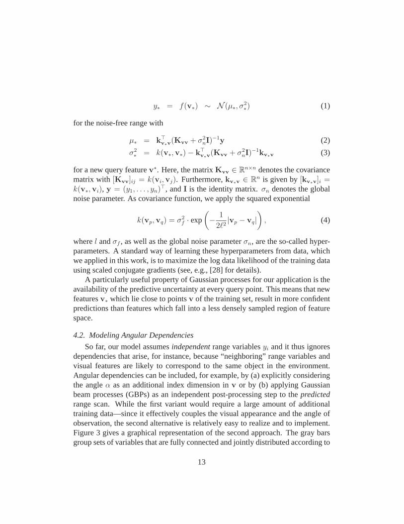
We applied this extended reflection probability mapping approach to the tra-jectories and range predictions that resulted from the experiments reported above.Figure 13 presents the laser-based maps using a standard reflection probabilitymapping system (left column) and our extended variant usingthe predicted ranges(right column) for the two environments (Freiburg on top andSaarbrucken below).In both cases, it is possible to build an accurate map, which is comparable to mapsobtained with infrared proximity sensors [36] or sonars [21].

6. Conclusion

This paper presents a new approach to estimating the free space around a robotbased on single images recorded with an omnidirectional camera. The task of es-timating the range to the closest obstacle is achieved by applying a Gaussian pro-cess model for regression, utilizing edge-based features extracted from the imageor, alternatively, using PCA or LDA to find a low-dimensional representation ofthe visual input in an unsupervised manner. All learned models outperform theoptimized individual features.

We furthermore showed in experiments with a real robot that the range pre-dictions are accurate enough to feed them into a mapping algorithm consideringpredictive range distributions and that the resulting mapsare comparable to mapsobtained with infrared or sonar sensors.

Acknowledgments

We would like to thank Andrzej Pronobis and Jie Luo for creating the CoSydata sets. This work has partly been supported by the EC undercontract numberFP7-231888-EUROPA and FP6-004250-CoSy, by the DFG under contract num-ber SFB/TR-8, and by the German Ministry for Education and Research (BMBF)through the DESIRE project.

23

Figure 13: Maps of the Freiburg AIS lab (top row) and DFKI Saarbrucken (bottom row) using reallaser data (left) and the predictions of theFeature-GP(right).

References

[1] G. Swaminathan, S. Grossberg, Laminar cortical mechanisms for the percep-tion of slanted and curved 3-D surfaces and their 2-D pictorical projections,Journal of Vision 2 (7) (2002) 79–79.

[2] A. Saxena, S. Chung, A. Ng., 3-d depth reconstruction froma single stillimage, Int. Journal of Computer Vision (IJCV).

[3] C. Plagemann, K. Kersting, P. Pfaff, W. Burgard, Gaussian beam processes:A nonparametric bayesian measurement model for range finders, in: Proc.of Robotics: Science and Systems (RSS), 2007.

[4] F. Sinz, J. Quinonero-Candela, G. Bakir, C. Rasmussen, M. Franz, Learningdepth from stereo, in: 26th DAGM Symposium, 2004.

24

[5] D. Lowe, Distinctive image features from scale-invariant keypoints, Interna-tional Journal of Computer Vision 60 (2) (2004) 91–110.

[6] H. Bay, A. Ess, T. Tuytelaars, L. Van Gool, SURF: Speeded up robust fea-tures, Computer Vision and Image Understanding (CVIU) 110 (3)(2008)346–359.

[7] A. Davision, I. Reid, N. Molton, O. Stasse, Monoslam: Real-time singlecamera slam, IEEE Transaction on Pattern Analysis and Machine Intelli-gence 29 (6).

[8] H. Strasdat, C. Stachniss, M. Bennewitz, W. Burgard, Visualbearing-onlysimultaneous localization and mapping with improved feature matching, in:Fachgesprache Autonome Mobile Systeme (AMS), 2007.

[9] B. Micusik, T. Pajdla, Structure from motion with wide circular field of viewcameras, IEEE Transactions on Pattern Analysis and MachineIntelligence28 (7) (2006) 1135–1149.

[10] R. Sim, J. J. Little, Autonomous vision-based exploration and mapping us-ing hybrid maps and Rao-Blackwellised particle filters, in: Proc. of theIEEE/RSJ Int. Conf. on Intelligent Robots and Systems (IROS), 2006, pp.2082–2089.

[11] P. Favaro, S. Soatto, A geometric approach to shape fromdefocus, IEEETrans. Pattern Anal. Mach. Intell. 27 (3) (2005) 406–417.

[12] A. Torralba, A. Oliva, Depth estimation from image structure, IEEE Trans-actions on Pattern Analysis and Machine Learning.

[13] H. Dahlkamp, A. Kaehler, D. Stavens, S. Thrun, G. Bradski, Self-supervisedmonocular road detection in desert terrain., in: Proc. of Robotics: Scienceand Systems (RSS), 2006.

[14] J. Michels, A. Saxena, A. Ng, High speed obstacle avoidance using monoc-ular vision and reinforcement learning, in: Int. Conf. on Machine Learning(ICML), 2005, pp. 593–600.

[15] E. Menegatti, A. Pretto, A. Scarpa, E. Pagello, Omnidirectional vision scanmatching for robot localization in dynamic environments, IEEE Transactionson Robotics 22 (3) (2006) 523–535.

25

[16] D. Hoiem, A. Efros, M. Herbert, Recovering surface layout from an image,Int. Journal of Computer Vision (IJCV) 75 (1).

[17] F. Han, S.-C. Zhu, Bayesian reconstruction of 3d shapes and scenes from asingle image, in: IEEE Int. Workshop on Higher-Level Knowledge in 3DModeling and Motion Analysis, Washington, DC, USA, 2003, p. 12.

[18] E. Delage, H. Lee, A. Ng., Automatic single-image 3d reconstructions ofindoor manhattan world scenes., in: Proceedings of the 12thInternationalSymposium of Robotics Research (ISRR), 2005.

[19] R. Ewerth, M. Schwalb, B. Freisleben, Using depth features to retrievemonocular video shots, in: Proceedings of the 6th ACM international con-ference on Image and video retrieval (CIVR), ACM, New York, NY, USA,2007, pp. 210–217.

[20] H. Moravec, A. Elfes, High resolution maps from wide angle sonar, in:Proc. of the IEEE Int. Conf. on Robotics & Automation (ICRA), St. Louis,MO, USA, 1985, pp. 116–121.

[21] S. Thrun, A. Bucken, W. Burgard, D. Fox, T. Frohlinghaus, D. Hennig,T. Hofmann, M. Krell, T. Schimdt, Map learning and high-speed navigationin RHINO, in: AI-based Mobile Robots: Case studies of successful robotsystems, MIT Press, Cambridge, MA, 1998.

[22] K. Sabe, M. Fukuchi, J.-S. Gutmann, T. Ohashi, K. Kawamoto, T. Yoshiga-hara, Obstacle avoidance and path planning for humanoid robots using stereovision, in: Proc. of the IEEE Int. Conf. on Robotics & Automation (ICRA),New Orleans, LA, USA, 2004.

[23] P. Elinas, R. Sim, J. J. Little,σSLAM: Stereo vision SLAM using the rao-blackwellised particle filter and a novel mixture proposal distribution, in:Proc. of ICRA, 2006.

[24] C. Plagemann, F. Endres, J. Hess, C. Stachniss, W. Burgard,Monocularrange sensing: A non-parametric learning approach, in: Proc. of the IEEEInt. Conf. on Robotics & Automation (ICRA), Pasadena, CA, USA, 2008.

[25] E. Alpaydin, Introduction To Machine Learning, MIT Press, 2004.

26

[26] E. R. Davies, Laws texture energy in texture, in: MachineVision: Theory,Algorithms, Practicalities, Acedemic Press, 1997.

[27] F. Canny, A computational approach to edge detection, IEEE Trans. PatternAnalysis and Machine Intelligence (1986) 679–714.

[28] C. Rasmussen, C. Williams, Gaussian Processes for MachineLearning, MITPress, 2006.

[29] C. Stachniss, C. Plagemann, A. Lilienthal, W. Burgard, Gasdistributionmodeling using sparse gaussian process mixture models, in:Proc. ofRobotics: Science and Systems (RSS), Zurich, Switzerland, 2008.

[30] V. Tresp, Mixtures of gaussian processes, in: Proc. of the Conf. on NeuralInformation Processing Systems (NIPS), 2000.

[31] EU Project CoSy. [link].URL http://www.cognitivesystems.org/

[32] S. Roweis, L. Saul, Nonlinear dimensionality reductionby locally linear em-bedding, Science 290 (5500) (2000) 2323–2326.

[33] J. Tenenbaum, V. de Silva, J. Langford, A global geometric framework fornonlinear dimensionality reduction., Science 290 (5500) (2000) 2319–2323.

[34] H. Chang, D.-Y. Yeung, Robust locally linear embedding, Pattern Recogni-tion 39 (6) (2006) 1053–1065.

[35] W. Burgard, C. Stachniss, D. Haehnel, Autonomous Navigation in Dy-namic Environments, Vol. 35 of STAR Springer tracts in advanced robotics,Springer Verlag, 2007, Ch. Mobile Robot Map Learning from RangeDatain Dynamic Environments.

[36] Y. Ha, H. Kim, Environmental map building for a mobile robot using infraredrange-finder sensors, Advanced Robotics 18 (4) (2004) 437–450.

27