42nd AIAA Aerospace Sciences Meeting and Exhibit 5-8 January 2004/ Reno, NV

1 American Institute of Aeronautics and Astronautics

A NON-BODY CONFORMAL GRID METHOD FOR SIMULATION OF COMPRESSIBLE FLOWS WITH COMPLEX IMMERSED BOUNDARIES

Reza Ghias*, Rajat Mittal†

Department of Mechanical and Aerospace Engineering The George Washington University, Washington, DC 20052

and Thomas S. Lund‡

Department of Aerospace Engineering Sciences The University of Colorado at Boulder, Boulder, CO 80309-0429

ABSTRACT

A compressible non-body conformal grid method is presented. The method is designed to simulate a large variety of subsonic compressible flows with complex geometries. A hybrid implicit-explicit time-discretization scheme is chosen. The diagonal viscous terms are treated implicitly and all other terms including the convective terms and cross-terms are treated explicitly using a low-storage, 3rd-Order Runge-Kutta scheme. A mixed second-order central difference-QUICK scheme has been used which allows us to precisely control the numerical damping. A ghost-cell approach is employed in conjunction with a bilinear interpolation scheme so as to satisfy the boundary conditions on the immersed boundaries while preserving second-order accuracy. Numerical results are validated by comparing against experimental data and other established simulation results.

INTRODUCTION

The conventional structured-grid approach to simulating flows with complex immersed boundaries is to discretize the governing equations on a curvilinear grid that conforms to the boundaries. Since the boundary itself becomes a grid line, the imposition of boundary conditions is greatly simplified and solver can be easily designed to maintain adequate accuracy and conservation properties. However depending on geometrical complexity of the immersed boundary, grid generation and grid quality can be major issues and one has resort to multi-block or other such approaches in order to handle anything but the simplest geometries. A different approach is to use simple Cartesian grids which do not conform to the immersed boundaries. This greatly simplifies the grid generation and moreover has * Student Member AIAA, Graduate Research Assistant † Associate Professor, Senior Member AIAA. ‡ Visiting Professor, Member AIAA.

great advantages with respect to conventional body- fitted methods in simulating flows with moving boundaries, complicated shapes, or topological changes1. Since the immersed boundary can cut through the underlying mesh in an arbitrary manner, the main challenge is to treat the boundary in a way that does not adversely impact the accuracy and conservation property of the underlying solver2. This is especially critical for viscous flows where inadequate resolution of boundary layers which form on the immersed boundaries, can reduce the fidelity of the numerical solution. The immersed boundary method (IBM) has recently gained popularity for simulating flows with complex geometries. In the original version of this method3, a localized body force was introduced in order to simulate the presence of boundaries without altering the computational grid. Subsequently a number of different variations of this methodology have been proposed4,5,6,7 and employed successfully to simulate a variety of flows. A somewhat different approach to simulating flows with complex immersed boundaries is to account for the boundary through direct modification of the discretized equations near the immersed boundary. So called “Cartesian grid methods”8 fall in this category. A finite-volume version of this method for simulating two-dimensional, unsteady, viscous, incompressible flows over complex geometries was developed by Ye et al.9 In these methods, instead of using the concept of momentum forcing, the finite-volumes near the body were reshaped into a mosaic of boundary-fitted trapezoidal cells. An interpolation procedure was then employed that maintained local and global second-order spatial accuracy. Furthermore, mass and momentum conservation were satisfied exactly irrespective of the mesh resolution. One issue faced with Cartesian grid based immersed boundary methods is that the grid size can grow much more rapidly with Reynolds number than a

2 American Institute of Aeronautics and Astronautics

corresponding structured curvilinear body-conformal mesh. Thus, for high Reynolds number simulations, it is worthwhile to develop immersed boundary type methods that can be employed in conjunction with curvilinear structured grids. Such methods allow us to provide localized resolution to the boundary layers on the immersed boundary while still retaining the flexibility of a non-body conformal grid. In the current paper, we describe a finite-difference based method that allows us to simulate subsonic compressible flows with complex immersed boundaries on Cartesian or curvilinear grids that do not conform to the immersed boundary. The method is based on the calculation of the variables on “ghost-cells” inside the body such that the boundary conditions are satisfied on the immersed boundary. There are no ad-hoc constants introduced in this procedure and neither is any momentum forcing employed in any of the fluid cells. Two and three-dimensional flow past a circular cylinder has been simulated over a range of Reynolds numbers in order to validate the approach and numerical procedure. Since the ultimate objective of this work is to simulate tip-flow of a helicopter rotor in hover, we present some results of flow past airfoils and wings as well. Governing Equations The governing equations are unsteady, viscous, compressible Navier-Stokes equations written in terms of conservative variables. The continuity, momentum and energy equations are:

( ) 0=∂∂

+∂∂

kk

uxt

ρρ

( ) ( ) 0=−+∂∂

+∂∂

ikikkkk

i puux

ut

σδρρ

( )[ ] 0=+−+∂∂

+∂∂

kiikkk

Qupeux

et

σ

where, the molecular heat flux and stress tensor are given by

( ) kk x

TQ

∂∂

−−=

PrRe1γγ

j

jik

i

k

k

iik x

u

xu

xu

∂

∂−

∂∂+

∂∂= δσ

Re1

32

Re1

respectively. In the above equations, Pr is the Prandtl number and Re is the Reynolds number. The velocity components and the pressure are related to the total energy per unit volume through the equation of state for a perfect gas by

( ) kk uup

e ργ 2

11

+−

=

The equations are transformed to a generalized curvilinear coordinate system, ( )ζηξ ,, while maintaining strong conservation form10.of the equations.

NUMERICAL METHODOLOGY

The equations are discretized in the computational domain with a cell-centered arrangement using a hybrid second-order central-difference-QUICK scheme11, which allows us to precisely control the numerical dissipation. The diagonal viscous terms are treated implicitly using a Crank-Nicolson scheme wherein all the other terms including the convective terms and cross-terms are treated explicitly using a low-storage, 3rd –order Runge-Kutta scheme.12 Use of this mixed implicit-explicit scheme virtually eliminates the viscous stability constraint which can be quite severe in simulation of viscous flows. The resulting equations are solved by a LSOR 12 iterative method Inclusion of Immersed Boundaries The geometry of immersed boundary is defined by a set of marker points. Cells whose centers lie inside the immersed body and have at least one neighboring cell whose cell-center lies outside the body, are marked as “ghost-cells”. The rest of the cells with centers inside the body, which are not adjacent to immersed boundary, are marked as “solid” cells. Fig.1 shows the marker points, fluid cells, ghost cells and solid cells for an immersed boundary on a Cartesian grid. The basic idea in this method is to compute the flow variables for the ghost cells such that boundary conditions on the immersed boundary in the vicinity of the ghost cell are satisfied. To compute the value at ghost cell center, a “normal probe” is extended from this node to the immersed boundary (to a point called “boundary-intercept” point) and is extended further into the fluid to a point which we call the “probe-tip”. Four cell centers (in 2D) which surround the probe-tip are then identified and a bilinear interpolation is employed in the computational domain to calculate the values at the probe-tip. The variables at the corresponding ghost node are subsequently computed by extrapolating them from the probe-tip and boundary-intercept points such that they satisfy appropriate Dirichlet or Neumann’s boundary conditions on the boundary-intercept point. Two approaches are used based on if four cell centers which surround the tip- marker point include the ghost cell center or not. Figs. 2.a and 2.b show these two approaches schematically. A systematic grid refinement study showed that this methodology maintains local and global second-order accuracy.

3 American Institute of Aeronautics and Astronautics

For flow with complex but stationary boundaries, generalization of the Cartesian grid approach to non body-conformal curvilinear grids can significantly enhance the power of the Cartesian grid approach. On the other hand, by not requiring the grid to conform precisely to the boundary, the grid generation requirements for complex geometries can be eased significantly and, the use of a curvilinear mesh can allow more control over the grid resolution in localized regions such as boundary layers. Consider for example the tip-flow of a rotor in hover which is the ultimate objective of the current project. Such flows are typically simulated on relatively complex multi-block C-H type of grids13, which conform to the shape of the rotor. However by using a non body-conformal grid, the grid topology can be greatly simplified (Fig. 3). This has been demonstrated in tip-clearance flow simulations carried out by You et al.14, where an immersed boundary method is used in conjunction with an incompressible flow solver to simulate tip-clearance flow in an axial turbo machine. Flow Configurations A circular cylinder is placed inside a large rectangular domain so as to minimize the boundary effects on the flow development. The flow is compressible with constant viscosity and specific heat ratio. At the inflow, all velocity components as well as the temperature are imposed, while the density is extrapolated from the domain and pressure is calculated by using the equation of state. At the outflow, a non-reflecting Navier-Stokes characteristic boundary condition15 (NSCB), is used which allows vortex structures to exit the computational domain with minimal spurious reflections. The lateral boundaries are treated as moving walls and density and temperature are determined by assuming adiabatic wall condition. The no-slip condition is imposed at the surface of circular cylinder. A periodic boundary condition is employed in the spanwise direction in the 3D circular cylinder simulations.

NUMERICAL RESULTS AND DISCUSSION

In this section we present results of 2D and 3D simulations of flow past a circular cylinder as well as airfoil and wing-tip simulations. 2D Cylinder Simulations Two-dimensional flow past a circular cylinder is simulated at Reynolds number of 100, 300 and 3900. The freestream Mach number for all these simulations is kept at a relatively low value of 0.3. For Re=100 and 300, a curvilinear grid with 459× 261(Fig.4) grid points was employed whereas for Re=3900 , a

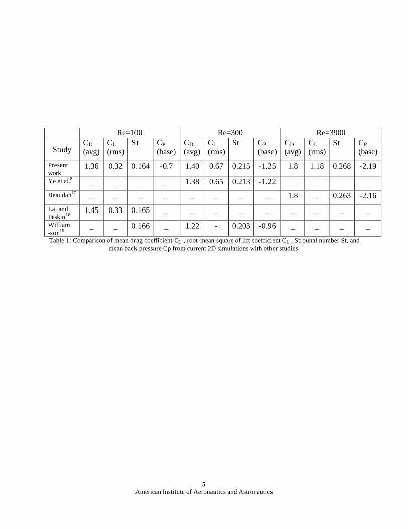
549× 385 curvilinear grid was used. Note that at Reynolds number greater than about 180, the flow past a circular cylinder is intrinsically three-dimensional and therefore 2D simulations at these Reynolds are not expected to produce flow fields that would match corresponding experiments. The computed flow can however still be validated against other 2D simulations. Fig. 5 shows the instantaneous vorticity contours plots in the near the wake of the circular cylinder for Re=100, 300 , and 3900. Distinct vortices associated with the Karman vortex street are observed and these visualizations indicate that the current methodology does reproduce the evolution of the vorticity fields with minimal spurious dissipation. Fig 6, 7, and 8 show the variation of lift and drag coefficients with time for Re=100,300 , and 3900 respectively. The lift and drag forces have been time averaged over a number of shedding cycles. Table 1, summarizes some key results obtained from the current 2D simulations and comparison with other corresponding experimental and numerical results. Note that in this table, the vortex shedding Strouhal number St is defined as

∞= UdfSt /

where f is the vortex shedding frequency. The results for Re=100 are found to be in good agreement with the experimental results. For Re=300 and 3600, the results are seen to be in reasonable agreement with other 2D simulations. This provides some quantitative validation of the current numerical methodology. 3D Cylinder Simulation One 3D simulation of flow past a circular cylinder at Re=300 have been carried out on a 143× 97× 49 (Fig. 9 ) Cartesian grid. The spanwise domain size is chosen to be 3d. The 3D simulation is initiated by using a corresponding 2D flow field and introducing a small amplitude spanwise perturbation in the flow field for a very short time. The 3-D perturbations evolve naturally and a saturated three-dimensional state is reached. Fig 10 shows iso-surfaces of enstrophy in the wake at one time-instant and flow structures similar to those in the DNS by Mittal and Balachandar16.are observed. Fig 11 shows a similar plot for the Re=3900 simulation. For this simulation, the spanwise domain size was d and a 549× 385× 33 grid was employed. It should be pointed out that a grid refinement study was performed to analyze the accuracy of the current method. Grid sizes of 1260× 1260, 420× 420, 252× 252, and 84× 84 were employed to simulate flow past a circular cylinder on a Cartesian grids at Re= 20. Fig.12 shows the log-log of the error for u component

4 American Institute of Aeronautics and Astronautics

velocity versus grid space. The plot clearly shows that second-order spatial accuracy is maintained. Airfoil and Wing-Tip Simulations Our goal in developing this numerical solver is to simulate the tip-flow of a rotor in hover. Therefore, in order to examine the performance of this method for airfoil-type geometries we have performed some preliminary simulations of 2D airfoil flows as well as well as wing-tip flow. Fig.13 shows a sequence of vorticity plots for a 2D NACA0012 airfoil flow at chord Reynolds number of 1.5×104 and M = 0.4 with 8 degree angle-of-attack. This simulation has been carried out on a 455 x 230 (Fig. 14) curvilinear grid. A tip-flow simulation was carried out at a relatively low Reynolds number of 5000 The X-Y grid (fig.3) was extended in spanwise direction and a 455× 230× 61 grid was employed. Fig.15 shows the tip-vortices contours at x=0.05 from the tail and Fig. 16 shows the streamlines for this simulation. The solver has recently been parallelized using Message Passing Interface (MPI) and this allows us to run the simulations on Pentium based Beowulf clusters with massively distributed memory . Using clusters with up to 16 CPU, we are currently carrying out simulations of the tip-flow at higher Reynolds number and results from these simulations will be presented in the future.

ACKNOWLEDGEMENT This research is being supported by the U.S. Army Research Office Grant No. 19-01-1-0704 monitored by Dr. T. Doligalski.

REFERENCES 1W. Shyy, H. S. Udaykumar, M. M. Rao, and R. W.

Smith, Computational Fluid Dynamics with Moving Boundaries,Taylor & Francis, London, 1996.

2Ye, R. Mittal, H.S. Udaykumar, W. Shyy, A Cartesian grid method for simulation of viscous incompressible flow with complex immersed boundaries, AIAA 99-3312

3Peskin, C. S., Flow patterns around the heart valves, J. Comput. Phys. , 10 (1972), 252-271.

4Goldstine, D., Handler, R., and Sirovich, L. , Modeling an no-slip flow boundary with an external

force field., J. Comput. Phys., 105 (1993), 345-366. 5Saiki, E. M., and Biringen, S., Numerical simulation of

a cylinder in uniform flow: application of a virtual boundary method., J. Comput. Phys., 123 (1996), 450-465.

6Mohd-Yusof, J., Combined immersed boundary /B-Spline methods for simulations of flow in complex geometries, CTR Annual Research Briefs, NASA Ames/Stanford University, (1997), 317-327.

7Fadlun, E. A., Verzicco, R., Orlandi, P., and Mohd-Yusof, J., Combined immersed boundary finite-difference methods for three-dimensional complex flow simulations., J. Comput. Phys., 161 (2000), 30-60.

8Ye. T., Mittal R., Udaykumar H. S., Shyy, W. Cartesian Grid Method for Simulation of Viscous Incompressible Flow with Complex Immersed Boundaries, AIAA 99-3312.

9Ye. T., Mittal, R., Udaykumar, H. S., and Shyy, W., An accurate Cartesian grid method for viscous incompressible flows with complex boundaries., J. Comput. Phys., 156 (1999), 209.

10Anderson, A.D., Tannehill, C.J., and Pletcher, R.H., Computational Fluid Mechanics and Heat Transfer, Hemispher Publishing Corporation, New York, 1984, 479-482.

11Leonard, B. P., A stable and accurate on convection modeling procedure based on quadratic upstream interpolation. Computer Methods in Applied Mechanics and Engineering , 19 (1979), 59-98

12Kennedy, C. A., Carpenter, M. A., and Lewis, R. M., Low-storage, explicit Runge-Kutta scheme for the compressible Navier-Stokes equations. ICASE Report No. 99-22(1999)

13Strawn, R. C., Duque, E. P., and Ahmad, J.,Rotorcraft aeroacoustics computations with overset-grid CFD methods., J. of the American Helicopter Socity, 44,(2) 1999, 132-140.

14You, D., Wang, M., Mittal, R., Moin, P., Study of rotor tip-clearance flow using large eddy simulation, AIAA (2003)- 838

15Poinsot, T. J., and Lele, S. K., Boundary conditions for direct simulations of compressible viscous flows, J. Comput. Phys., 101(1992), 104-129

16Mittal, R., Balachandar, S., On the inclusion of three-dimensional effects in simulations of two-dimensional bluff-body wake flows., Symposium on separated and complex flows, ASME Summer meeting , Vancouver, (1997).

17Beaudan, P., and Moin, P., Numerical experiments on the flow past a circular cylinder at sub-critical Reynolds number., report No. TF-62, Thermo-sciences Division, Department of Mechanical Engineering, Stanford University, (1994).

18Lai, M. C., and Peskin, C. S., An immersed boundary method with formal second-order accuracy and reduced numerical viscosity., J. Comput. Phys., 160 (2000), 705-719.

19Williamson, C. H. K., Vortex dynamics in the cylinder wake, Ann. Rev. Fluid Mech., 8(1996), 477-539.

5 American Institute of Aeronautics and Astronautics

Re=100 Re=300 Re=3900

Study CD (avg)

CL (rms)

St CP (base)

CD (avg)

CL (rms)

St CP (base)

CD (avg)

CL (rms)

St CP (base)

Present work

1.36 0.32 0.164 -0.7 1.40 0.67 0.215 -1.25 1.8 1.18 0.268 -2.19

Ye et al.8 _ _ _ _ 1.38 0.65 0.213 -1.22 _ _ _ _

Beaudan17 _ _ _ _ _ _ _ _ 1.8 _ 0.263 -2.16

Lai and Peskin18

1.45 0.33 0.165 _ _ _ _ _ _ _ _ _

William -son19

_ _ 0.166 _ 1.22 - 0.203 -0.96 _ _ _ _

Table 1: Comparison of mean drag coefficient CD , root-mean-square of lift coefficient CL , Strouhal number St, and mean back pressure Cp from current 2D simulations with other studies.

AIAA 2004-0080

6 American Institute of Aeronautics and Astronautics

Figure 1: Marker points, flow nodes, ghost nodes and solid nodes in a Cartesian grid

( a ) (b) Figure.2:(a): Tip marker point is surrounded by four nodes including ghost node. (b): Tip marker point is surrounded

by four nodes not including ghost node.

Marker pointFlow node

Ghost node Solid node

Tip marker

Normal point

Normal line

Tip marker

Normal point

Normal line

AIAA 2004-0080

7 American Institute of Aeronautics and Astronautics

Fig.3: The non-body conformal grid used in the tip-flow Fig.4: The Rectangular curvilinear domain in X-Y plan. Grid size is 459× 261× 33. Fig. 5: Vorticity contours at one time -instant for Fig.6: The lift and drag coefficients at Re=100 as a (a) Re=100, (b) Re=300, (c) Re=3900. function of time, where time =tU8 /d and M =0.3

-15

-10

-5

0

5

10

15

Y

-20 -10 0 10 20X

X

Y

Z

XZ

X

Y

Z

time

CL/

CD

Coe

ff.

100 120 140 160 180 200-1

-0.5

0

0.5

1

1.5

AIAA 2004-0080

8 American Institute of Aeronautics and Astronautics

Fig. 7: The lift and drag coefficients at Re=300 as a Fig. 8: The lift and drag coefficients at Re=3900 as function of time, where time =tU8 /d and M =0.3 function of time, where time= tU8 /d and M =0.3

Fig.9: The rectangular Cartesian grid domain Fig. 10: Isosurface of instantaneous cross vorticity

in X-Y plan. Grid size is 143 × 97× 49 22yx ωω + at Re=300, and M=0.3

time

CL/

CD

Coe

ff.

200 220 240-2

-1.5

-1

-0.5

0

0.5

1

1.5

2

ClCD

timeC

L/C

DC

oeff.

35 40 45-3

-2

-1

0

1

2

3

ClCD

X

Y

Z

X

Y

Z

AIAA 2004-0080

9 American Institute of Aeronautics and Astronautics

Fig. 11: Iso-surface of instantaneous cross vorticity Fig. 12: Log-log error of u velocity component

22yx ωω + at Re=3900, and M = 0. 3 versus grid spacing.

Fig.13: Sequence of spanwise vorticity contours, Fig.14: The Rectangular curvilinear domain showing the unsteady separation in for tip- flow simulation in X-Y plan . NACA0012 airfoil at Red = 1.5 ×104, Grid size is 455× 230× 61 M = 0.4, and angle-of-attack of 8 degrees.

X

Y

Z

AIAA 2004-0080

10 American Institute of Aeronautics and Astronautics

Fig15: Tip-flow cross vorticity contours of 22

yx ωω + Fig. 16: Stream lines for tip-flow in rectangular

at x=0.05 for rectangular NACA0012, NACA0012, Re=5000, M =0.4 Re = 5000, M =0.4, and angel of attack=8°. Contours from 0.2 to 4.

X

Y

Z

X

Y

Z