A New View of the Bacterial Cytosol Environment

A New View of the Bacterial Cytosol EnvironmentBenjamin P. Cossins1, Matthew P. Jacobson2, Victor Guallar1*

1 Department of Life Science, Barcelona Supercomputer Center, Barcelona, Spain, 2 Department of Pharmaceutical Chemistry, University of California San Francisco, San

Francisco, California, United States of America

Abstract

The cytosol is the major environment in all bacterial cells. The true physical and dynamical nature of the cytosol solution isnot fully understood and here a modeling approach is applied. Using recent and detailed data on metaboliteconcentrations, we have created a molecular mechanical model of the prokaryotic cytosol environment of Escherichia coli,containing proteins, metabolites and monatomic ions. We use 200 ns molecular dynamics simulations to compute diffusionrates, the extent of contact between molecules and dielectric constants. Large metabolites spend ,80% of their time incontact with other molecules while small metabolites vary with some only spending 20% of time in contact. Large non-covalently interacting metabolite structures mediated by hydrogen-bonds, ionic and p stacking interactions are commonand often associate with proteins. Mg2+ ions were prominent in NIMS and almost absent free in solution. K+ is generally notinvolved in NIMSs and populates the solvent fairly uniformly, hence its important role as an osmolyte. In simulationscontaining ubiquitin, to represent a protein component, metabolite diffusion was reduced owing to long lasting protein-metabolite interactions. Hence, it is likely that with larger proteins metabolites would diffuse even more slowly. Thedielectric constant of these simulations was found to differ from that of pure water only through a large contribution fromubiquitin as metabolite and monatomic ion effects cancel. These findings suggest regions of influence specific to particularproteins affecting metabolite diffusion and electrostatics. Also some proteins may have a higher propensity for associationswith metabolites owing to their larger electrostatic fields. We hope that future studies may be able to accurately predicthow binding interactions differ in the cytosol relative to dilute aqueous solution.

Citation: Cossins BP, Jacobson MP, Guallar V (2011) A New View of the Bacterial Cytosol Environment. PLoS Comput Biol 7(6): e1002066. doi:10.1371/journal.pcbi.1002066

Editor: Emad Tajkhorshid, University of Illinois, United States of America

Received November 13, 2010; Accepted April 9, 2011; Published June 9, 2011

Copyright: � 2011 Cossins et al. This is an open-access article distributed under the terms of the Creative Commons Attribution License, which permitsunrestricted use, distribution, and reproduction in any medium, provided the original author and source are credited.

Funding: This work was supported by computational resources and funds from the Barcelona Supercomputer Center and through the Spanish Ministry ofEducation and Science through the project CTQ2007-62122/BQU. The funders had no role in study design, data collection and analysis, decision to publish, orpreparation of the manuscript.

Competing Interests: The authors have declared that no competing interests exist.

* E-mail: [email protected]

Introduction

The composition of metabolites, ions and proteins, and

processes such as metabolism and signalling which take place in

the E.coli cytosol are largely well defined [1,2]. However, the

structure and dynamical nature of the cytosol solution is less well

understood whether on the local or cytosol-wide levels. Current

perception of the cytosol solution is often of a unstructured

mixture with behaviour that differs quantitatively but not

qualitatively from an ideal solution. Alternatively, there are

theoretical descriptions of a cytosol organised into functionally

specific regions and even separated protein and small molecule

regions linked by metabolite transit pathways [3,4].

Cytosolic metabolites are extremely varied, but a large majority

of these molecules are negatively charged. Assumed electro-

neutrality is maintained by a large concentration of potassium ions

and to a lesser degree by magnesium and poly-amines such as

putrescine and spermidine. The large amount of charge in the

cytosol suggests that electrostatics is a dominant force. However,

the Debye length at physiological ionic strength is very short (less

than 1 nm) [3,4]. This electrostatic screening is probably essential

for the observed extent of macromolecular crowding [5].

The charge distribution and dynamics of the solution also

determines the dielectric constant (e), which is reduced by

increasing concentration of monatomic ions [6,7] while

Zwitterionic metabolites are thought to increase e [8–10]. The

effect of proteins seems to vary, with some studies suggesting an

increment [11–13] and others a decrement [14,15]. Experi-

mental data on e of the cytosol is sparse but in general it suggests

that cytosolic e is significantly larger than that for pure water

[16–19].

The hydrophobic effect is also significantly modulated by ionic

strength. Increasing salt concentration increases the strength of the

hydrophobic effect [20] possibly through the weakening of water

hydrogen bonding [21]. Almost all theoretical treatments of these

issues assume simple solutions of monatomic ions and water,

sometimes at infinite dilution. There has been little examination of

differences in solutions containing positive monatomic ions and

larger, negatively charged solutes.

Given the complexity of the cytosol environment it is very

difficult to predict the true nature of structure, dynamics and

thermodynamics. With a high level of electrostatic screening and

heightened hydrophobicity, is it likely that metabolites and

proteins engage in significant and long lasting interactions? A

recent theoretical study has attempted to make sense of non-ideal

behaviour for two component solutions of some common organic

molecules [22]. For some mixtures it was shown that activity can

actually decrease with increasing concentration, suggesting a high

level of non-ideal behavior. Another study found significantly

lower thermodynamic activities between in vivo like and standard

PLoS Computational Biology | www.ploscompbiol.org 1 June 2011 | Volume 7 | Issue 6 | e1002066

conditions for enzyme-inhibitor assays, again suggesting significant

non-ideal behaviour [23].

Using a recent extensive list of metabolites and their

concentrations from exponentially growing E. coli [24], we have

produced two types of atomistic molecular dynamics simulations of

a simplified cytosolic model. One included metabolites only and

another also included a protein component, for which we used

ubiquitin. Although ubiquitin (PDB code 1UBQ) is a eukaryotic

protein, it was chosen owing to its small size and large amount of

literature dedicated to its study [25–27]. Molecular dynamics

allowed us to compute several properties of interest, including e,

amount of contact between cytosolic molecules and diffusion

coefficients. The simulations indicate that metabolites spend a

large proportion of their time as part of ‘non-covalently interacting

metabolite structures’ (NIMS). Our results also indicate that the

cytosolic e is larger than that of water with monatomic ions. These

data allow us to make suggestions about the global structure of the

cytosol and the amount of time different metabolites spend free in

solution.

Results

Structural analysisThis study involved two large cytosol simulations with cubic

boxes of 100 A dimensions, one containing metabolites with

monatomic ions (100M) and another with four additional

ubiquitin molecules (100MP). Two smaller cytosol simulations

(50M and 50MP), a pure water (tip3p) and water + KCl

(tip3p+KCl) all with *50 A dimensions were produced for the

dielectric analysis. For a complete list of the simulations of this

study and their simplified labels it is instructive to refer to table 1

and the methods section.

The structure of cytosol simulations quickly collapsed from

almost equal spacing of metabolites to a series of non-covalently

interacting metabolite structures (NIMS) inter-spaced with solvent,

ions and fully solvated metabolites. This process was conveniently

measured through solvent accessible surface area (SASA) of all

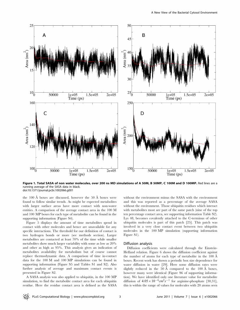
metabolites except monatomic ions (Figure 1).

Both 50 A simulations were deemed equilibrated after 30 ns

(Figure 1) while the 100M and 100 MP were equilibrated after 35

and 50 ns respectively. Hence, all analyses were carried out only

on this structurally equilibrated data (see supporting information

Figure S7). Around 16.7% of SASA is lost within the 50 MP

system which is similar to the 100 MP box where around 16.4% is

lost. These percentage values were calculated using the running

averages shown in red in Figure 1. The effect of the box size on

metabolite behaviour and general size of NIMS is difficult to gauge

but the fact that there is little relative difference between 100 and

50 A may suggest that smaller box sizes can be used for

computationally expensive calculations.

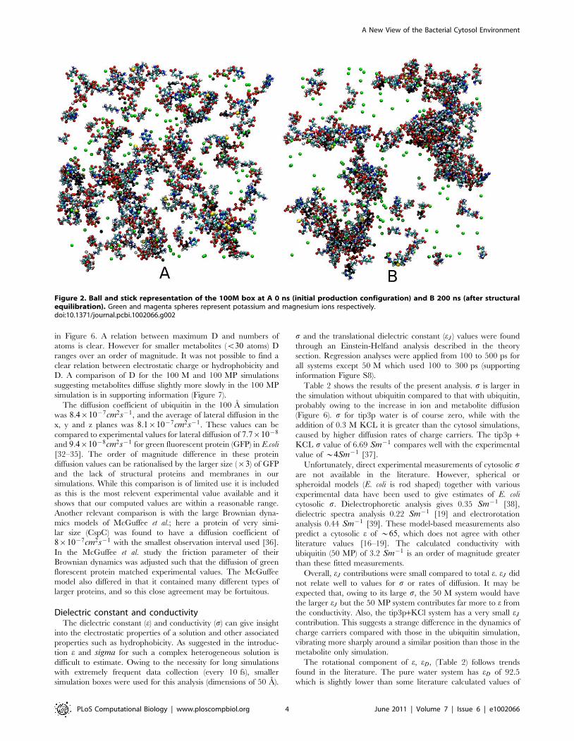
Figure 2 shows a view through the 100 M box at the beginning

of the production simulation and after 200 ns. It is clear that after

equilibration there is a significant difference in structure. Within

the 200 ns simulation of the 100 A boxes many NIMS were

formed which were stable over relatively long time periods. The

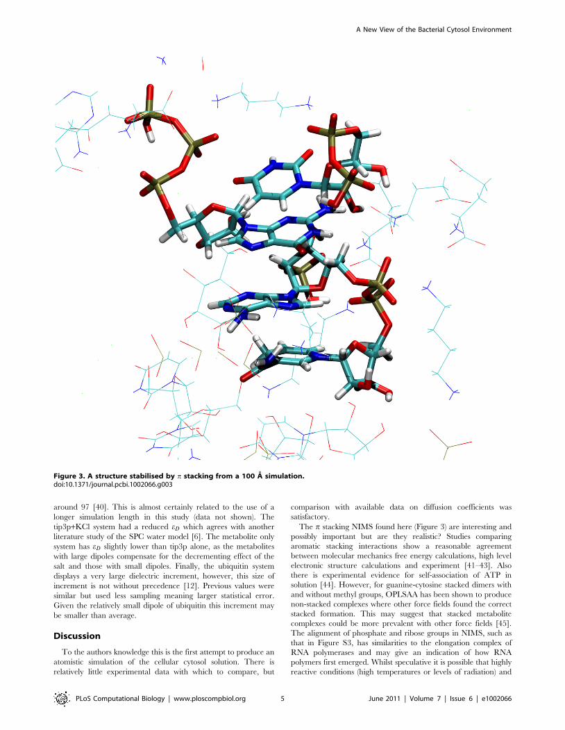
most interesting of these NIMS were those with a p stacking core

of nucleotide base like groups (Figure 3 A). These p stacks

continuously gain and lose bases and persist as long as 50 ns. Some

p stack NIMS seem reminiscent of RNA and we speculate that

these structures often show similarities with the elongation

complex of RNA polymerases [28] in the way phosphates are

aligned with ribose rings (Figure S3).

The inclusion of four ubiquitin molecules perturbed the

metabolite structures. Many large NIMSs became attached to

protein surface areas containing positively charged residues

(Figure 4), in many cases for time periods of 50–100 ns. The

attachment or detachment of large NIMS from the protein may

contribute to the large SASA fluctuations of Figure 1. These

protein-connected NIMSs can also form bridges connecting two

proteins which correlates their motions (Figure 4).

Interactions among metabolites and proteinsSASA analysis was used to investigate any propensity for

metabolites to interact. For the SASA and diffusion analyses, only

Table 1. Details of the size and numbers of molecules and atoms in each of four simulations used in this study.

Box dimension metabolites proteins K+ Mg2+ atoms

50M 45.4 19 0 22 3 9241

100M 90.85 157 0 175 27 73124

50MP 50.0 19 1 22 3 13636

100MP 100.0 157 4 175 27 98619

tip3p 50.0 0 0 0 0 13226

tip3pzKCl 50.0 0 0 26 0 13098

doi:10.1371/journal.pcbi.1002066.t001

Author Summary

The cytosol is the major cellular environment housing themajority of cellular activity. Although the cytosol is anaqueous environment, it contains high concentrations ofions, metabolites, and proteins, making it very differentfrom dilute aqueous solution, which is frequently used forin vitro biochemistry. Recent advances in metabolomicshave provided detailed concentration data for metabolitesin E.coli. We used this information to construct accurateatomistic models of the cytosol solution. We find that,unlike the situation in dilute solutions, most metabolitesspend the majority of their time in contact with othermetabolites, or in contact with proteins. Furthermore, wefind large non-covalently interacting metabolite structuresare common and often associated with proteins. Thepresence of proteins reduced metabolite diffusion owingto long lasting correlations of motion. The dielectricconstant of these simulations was found to differ fromthat of pure water only through a large contribution fromproteins as metabolite and monatomic ion effects largelycancel. These findings suggest specific protein spheres ofinfluence affecting metabolite diffusion and the electro-static environment.

A New View of the Bacterial Cytosol Environment


the 100 A boxes are discussed, however the 50 A boxes were

found to follow similar trends. As might be expected metabolites

with larger surface areas have more contact with non-water

entities. A comparison of the average contact area in the 100 M

and 100 MP boxes for each type of metabolite can be found in the

supporting information (Figure S4).

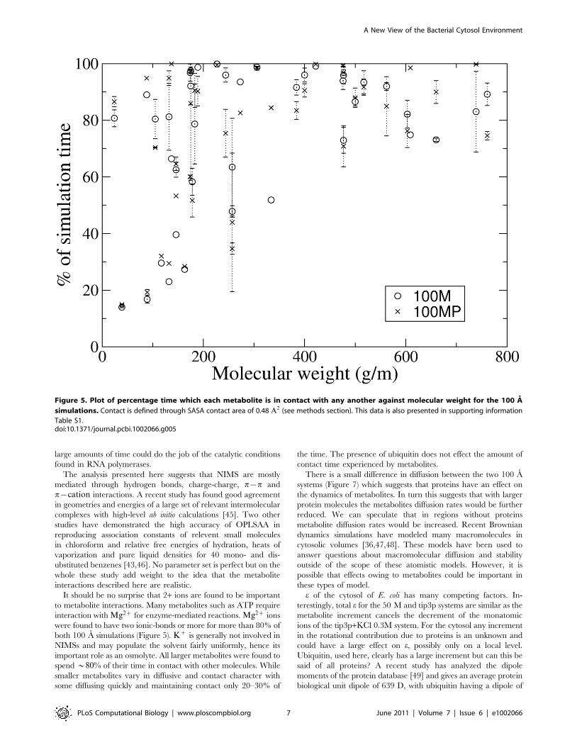
Figure 5 displays the amount of time metabolites spend in

contact with other molecules and hence are unavailable for any

specific interactions. The threshold for our definition of contact is

two hydrogen bonds or more (see methods section). Larger

metabolites are contacted at least 70% of the time while smaller

metabolites show much larger variability with some as low as 20%

and other as high as 95%. This analysis gives an indication of

metabolites availability for metabolism but of course cannot

replace thermodynamic data. A comparison of time in-contact

data for the 100 M and 100 MP simulations can be found in

supporting information (Figure S5 and Tables S1 and S2). Also

further analysis of average and maximum contact events is

presented in Figure S2.

A SASA analysis was also applied to ubiquitin, in the 100 MP

simulation, to find the metabolite contact area for each ubiquitin

residue. Here the residue contact area is defined as the SASA

without the environment minus the SASA with the environment

and this was reported as a percentage of the average SASA

without the environment. Those ubiquitin residues which interact

with metabolites most are part of the same patch (nine of the top

ten percentage contact area, see supporting information Table S2).

Lys 48, becomes covalently attached to the C-terminus of other

ubiquitin molecules is part of this patch [25]. This patch was

involved in a very close contact event between two ubiquitin

molecules in the 100 MP simulation (supporting information

Figure S1).

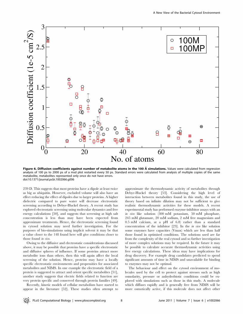
Diffusion analysisDiffusion coefficients were calculated through the Einstein-

Helfand relation. Figure 6 shows the diffusion coefficient against

the number of atoms for each type of metabolite in the 100 A

boxes. Recent work has shown a periodic box size dependence for

water diffusion in water [29]. Here some diffusion rates were

slightly reduced in the 50 A compared to the 100 A boxes,

however many were identical (Figure S6 of supporting informa-

tion). We have identified only one literature value for metabolite

diffusion of 4:05|10{6cm2s{1 for arginine-phosphate [30,31],

this is within the range of values for molecules with 20 atoms seen

Figure 1. Total SASA of non water molecules, over 200 ns MD simulations of A 50M, B 50MP, C 100M and D 100MP. Red lines are arunning average of the SASA data in black.doi:10.1371/journal.pcbi.1002066.g001



in Figure 6. A relation between maximum D and numbers of

atoms is clear. However for smaller metabolites (v30 atoms) D

ranges over an order of magnitude. It was not possible to find a

clear relation between electrostatic charge or hydrophobicity and

D. A comparison of D for the 100 M and 100 MP simulations

suggesting metabolites diffuse slightly more slowly in the 100 MP

simulation is in supporting information (Figure 7).

The diffusion coefficient of ubiquitin in the 100 A simulation

was 8:4|10{7cm2s{1, and the average of lateral diffusion in the

x, y and z planes was 8:1|10{7cm2s{1. These values can be

compared to experimental values for lateral diffusion of 7:7|10{8

and 9:4|10{8cm2s{1 for green fluorescent protein (GFP) in E.coli

[32–35]. The order of magnitude difference in these protein

diffusion values can be rationalised by the larger size (|3) of GFP

and the lack of structural proteins and membranes in our

simulations. While this comparison is of limited use it is included

as this is the most relevent experimental value available and it

shows that our computed values are within a reasonable range.

Another relevant comparison is with the large Brownian dyna-

mics models of McGuffee et al.; here a protein of very simi-

lar size (CspC) was found to have a diffusion coefficient of

8|10{7cm2s{1 with the smallest observation interval used [36].

In the McGuffee et al. study the friction parameter of their

Brownian dynamics was adjusted such that the diffusion of green

florescent protein matched experimental values. The McGuffee

model also differed in that it contained many different types of

larger proteins, and so this close agreement may be fortuitous.

Dielectric constant and conductivityThe dielectric constant (e) and conductivity (s) can give insight

into the electrostatic properties of a solution and other associated

properties such as hydrophobicity. As suggested in the introduc-

tion e and sigma for such a complex heterogeneous solution is

difficult to estimate. Owing to the necessity for long simulations

with extremely frequent data collection (every 10 fs), smaller

simulation boxes were used for this analysis (dimensions of 50 A).

s and the translational dielectric constant (eJ ) values were found

through an Einstein-Helfand analysis described in the theory

section. Regression analyses were applied from 100 to 500 ps for

all systems except 50 M which used 100 to 300 ps (supporting

information Figure S8).

Table 2 shows the results of the present analysis. s is larger in

the simulation without ubiquitin compared to that with ubiquitin,

probably owing to the increase in ion and metabolite diffusion

(Figure 6). s for tip3p water is of course zero, while with the

addition of 0.3 M KCL it is greater than the cytosol simulations,

caused by higher diffusion rates of charge carriers. The tip3p +KCL s value of 6.69 Sm{1 compares well with the experimental

value of *4Sm{1 [37].

Unfortunately, direct experimental measurements of cytosolic sare not available in the literature. However, spherical or

spheroidal models (E. coli is rod shaped) together with various

experimental data have been used to give estimates of E. coli

cytosolic s. Dielectrophoretic analysis gives 0.35 Sm{1 [38],

dielectric spectra analysis 0.22 Sm{1 [19] and electrorotation

analysis 0.44 Sm{1 [39]. These model-based measurements also

predict a cytosolic e of *65, which does not agree with other

literature values [16–19]. The calculated conductivity with

ubiquitin (50 MP) of 3.2 Sm{1 is an order of magnitude greater

than these fitted measurements.

Overall, eJ contributions were small compared to total e. eJ did

not relate well to values for s or rates of diffusion. It may be

expected that, owing to its large s, the 50 M system would have

the larger eJ but the 50 MP system contributes far more to e from

the conductivity. Also, the tip3p+KCl system has a very small eJ

contribution. This suggests a strange difference in the dynamics of

charge carriers compared with those in the ubiquitin simulation,

vibrating more sharply around a similar position than those in the

metabolite only simulation.

The rotational component of e, eD, (Table 2) follows trends

found in the literature. The pure water system has eD of 92.5

which is slightly lower than some literature calculated values of

Figure 2. Ball and stick representation of the 100M box at A 0 ns (initial production configuration) and B 200 ns (after structuralequilibration). Green and magenta spheres represent potassium and magnesium ions respectively.doi:10.1371/journal.pcbi.1002066.g002



around 97 [40]. This is almost certainly related to the use of a

longer simulation length in this study (data not shown). The

tip3p+KCl system had a reduced eD which agrees with another

literature study of the SPC water model [6]. The metabolite only

system has eD slightly lower than tip3p alone, as the metabolites

with large dipoles compensate for the decrementing effect of the

salt and those with small dipoles. Finally, the ubiquitin system

displays a very large dielectric increment, however, this size of

increment is not without precedence [12]. Previous values were

similar but used less sampling meaning larger statistical error.

Given the relatively small dipole of ubiquitin this increment may

be smaller than average.

Discussion

To the authors knowledge this is the first attempt to produce an

atomistic simulation of the cellular cytosol solution. There is

relatively little experimental data with which to compare, but

comparison with available data on diffusion coefficients was

satisfactory.

The p stacking NIMS found here (Figure 3) are interesting and

possibly important but are they realistic? Studies comparing

aromatic stacking interactions show a reasonable agreement

between molecular mechanics free energy calculations, high level

electronic structure calculations and experiment [41–43]. Also

there is experimental evidence for self-association of ATP in

solution [44]. However, for guanine-cytosine stacked dimers with

and without methyl groups, OPLSAA has been shown to produce

non-stacked complexes where other force fields found the correct

stacked formation. This may suggest that stacked metabolite

complexes could be more prevalent with other force fields [45].

The alignment of phosphate and ribose groups in NIMS, such as

that in Figure S3, has similarities to the elongation complex of

RNA polymerases and may give an indication of how RNA

polymers first emerged. Whilst speculative it is possible that highly

reactive conditions (high temperatures or levels of radiation) and

Figure 3. A structure stabilised by p stacking from a 100 A simulation.doi:10.1371/journal.pcbi.1002066.g003



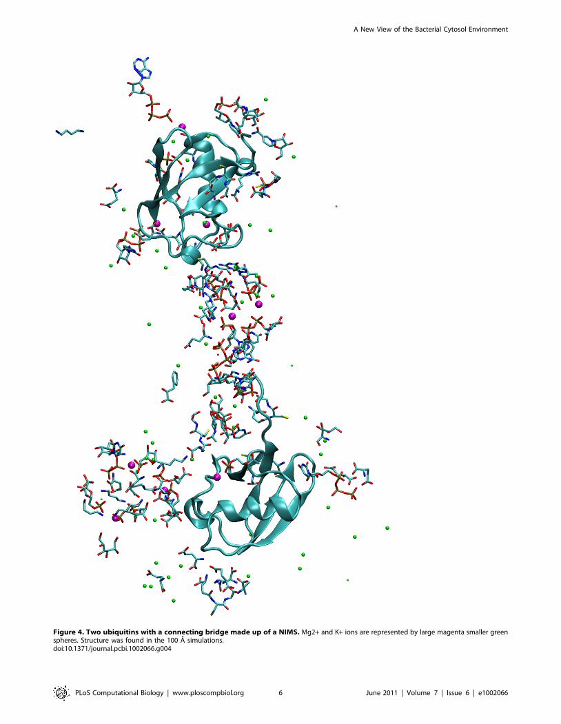
Figure 4. Two ubiquitins with a connecting bridge made up of a NIMS. Mg2+ and K+ ions are represented by large magenta smaller greenspheres. Structure was found in the 100 A simulations.doi:10.1371/journal.pcbi.1002066.g004



large amounts of time could do the job of the catalytic conditions

found in RNA polymerases.

The analysis presented here suggests that NIMS are mostly

mediated through hydrogen bonds, charge-charge, p{p and

p{cation interactions. A recent study has found good agreement

in geometries and energies of a large set of relevant intermolecular

complexes with high-level ab initio calculations [45]. Two other

studies have demonstrated the high accuracy of OPLSAA in

reproducing association constants of relevent small molecules

in chloroform and relative free energies of hydration, heats of

vaporization and pure liquid densities for 40 mono- and dis-

ubstituted benzenes [43,46]. No parameter set is perfect but on the

whole these study add weight to the idea that the metabolite

interactions described here are realistic.

It should be no surprise that 2+ ions are found to be important

to metabolite interactions. Many metabolites such as ATP require

interaction with Mg2z for enzyme-mediated reactions. Mg2z ions

were found to have two ionic-bonds or more for more than 80% of

both 100 A simulations (Figure 5). Kz is generally not involved in

NIMSs and may populate the solvent fairly uniformly, hence its

important role as an osmolyte. All larger metabolites were found to

spend *80% of their time in contact with other molecules. While

smaller metabolites vary in diffusive and contact character with

some diffusing quickly and maintaining contact only 20–30% of

the time. The presence of ubiquitin does not effect the amount of

contact time experienced by metabolites.

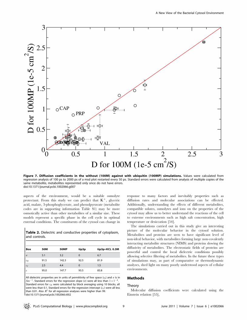
There is a small difference in diffusion between the two 100 A

systems (Figure 7) which suggests that proteins have an effect on

the dynamics of metabolites. In turn this suggests that with larger

protein molecules the metabolites diffusion rates would be further

reduced. We can speculate that in regions without proteins

metabolite diffusion rates would be increased. Recent Brownian

dynamics simulations have modeled many macromolecules in

cytosolic volumes [36,47,48]. These models have been used to

answer questions about macromolecular diffusion and stability

outside of the scope of these atomistic models. However, it is

possible that effects owing to metabolites could be important in

these types of model.

e of the cytosol of E. coli has many competing factors. In-

terestingly, total e for the 50 M and tip3p systems are similar as the

metabolite increment cancels the decrement of the monatomic

ions of the tip3p+KCl 0.3M system. For the cytosol any increment

in the rotational contribution due to proteins is an unknown and

could have a large effect on e, possibly only on a local level.

Ubiquitin, used here, clearly has a large increment but can this be

said of all proteins? A recent study has analyzed the dipole

moments of the protein database [49] and gives an average protein

biological unit dipole of 639 D, with ubiquitin having a dipole of

Figure 5. Plot of percentage time which each metabolite is in contact with any another against molecular weight for the 100 A

simulations. Contact is defined through SASA contact area of 0.48 A2 (see methods section). This data is also presented in supporting information

Table S1.doi:10.1371/journal.pcbi.1002066.g005



239 D. This suggests that most proteins have a dipole at least twice

as big as ubiquitin. However, excluded volume will also have an

effect reducing the effect of dipoles due to larger proteins. A higher

dielectric compared to pure water will decrease electrostatic

screening according to Debye-Huckel theory. A recent study has

explored electrostatic screening using molecular dynamics and free

energy calculations [50], and suggests that screening at high salt

concentration is less than may have been expected from

approximate treatments. Hence, the electrostatic screening found

in cytosol solution may need further investigation. For the

purposes of bio-simulations using implicit solvent it may be that

a value closer to the 148 found here will give conditions closer to

those found in vivo.

Owing to the diffusive and electrostatic considerations discussed

above, it may be possible that proteins have a specific electrostatic

and diffusive spheres of influence. If some proteins attract more

metabolite ions than others, then this will again affect the local

screening of the solution. Hence, proteins may have a locally

specific electrostatic environments and propensities for associated

metabolites and NIMS. In one example the electrostatic field of a

protein is suggested to attract and orient specific metabolites [51],

another study suggests that electric fields related to function are

very protein specific and conserved through protein families [49].

Recently, kinetic models of cellular metabolism have started to

appear in the literature [52]. These studies often attempt to

approximate the thermodynamic activity of metabolites through

Debye-Huckel theory [53]. Considering the high level of

interaction between metabolites found in this study, the use of

theory based on infinite dilution may not be sufficient to give

realistic thermodynamic activities for these models. A recent

experimental study has performed enzyme-inhibitor assays with an

in vivo like solution (300 mM potassium, 50 mM phosphate,

245 mM glutamate, 20 mM sodium, 2 mM free magnesium and

0.5 mM calcium, at a pH of 6.8) rather than a standard

concentration of the inhibitor [23]. In the in vivo like solution

some enzymes have capacities (Vmax) which are less than half

those found in optimised conditions. The solutions used are far

from the complexity of the real cytosol and so further investigation

of more complex solutions may be required. In the future it may

be possible to calculate accurate thermodynamic activities using

free energy calculations. These ideas may have implications for

drug discovery. For example drug candidates predicted to spend

significant amounts of time in NIMS and unavailable for binding

to enzymes may not be optimal.

The behaviour and effect on the cytosol environment of mo-

lecules used by the cell to protect against stresses such as high

osmolarity, pressure or anhydrobiotic conditions could be ex-

plored with simulations such as those in this study. A molecule

which diffuses rapidly and is generally free from NIMS will be

more osmotically active, if this molecule does not affect other

Figure 6. Diffusion coefficients against number of metabolite atoms in the 100 A simulations. Values were calculated from regressionanalysis of 100 ps to 2000 ps of a msd plot restarted every 50 ps. Standard errors were calculated from analysis of multiple copies of the samemetabolite, metabolites represented only once do not have errors.doi:10.1371/journal.pcbi.1002066.g006



aspects of the environment, would be a suitable osmolyte

protectant. From this study we can predict that Kz, glyceric

acid, malate, 3-phosphoglycerate, and phenolpyruvate (metabolite

codes are in supporting information Table S1) may be more

osmotically active than other metabolites of a similar size. These

models represent a specific phase in the cell cycle in optimal

external conditions. The constituents of the cytosol can change in

response to many factors and inevitably properties such as

diffusion rates and molecular associations can be effected.

Additionally, understanding the effects of different metabolites,

compatible solutes, osmolytes and ions on the properties of the

cytosol may allow us to better understand the reactions of the cell

to extreme environments such as high salt concentration, high

temperature or desiccation [54].

The simulations carried out in this study give an interesting

picture of the molecular behavior in the cytosol solution.

Metabolites and proteins are seen to have significant level of

non-ideal behavior, with metabolites forming large non-covalently

interacting metabolite structures (NIMS) and proteins slowing the

diffusivity of metabolites. The electrostatic fields of proteins are

powerful and control the local dielectric conditions possibly

allowing selective filtering of metabolites. In the future these types

of simulations may, as part of comparative or thermodynamic

analyses, shed light on many poorly understood aspects of cellular

environments.

Methods

TheoryMolecular diffusion coefficients were calculated using the

Einstein relation [55],

Figure 7. Diffusion coefficients in the without (100M) against with ubiquitin (100MP) simulations. Values were calculated fromregression analysis of 100 ps to 2000 ps of a msd plot restarted every 50 ps. Standard errors were calculated from analysis of multiple copies of thesame metabolite, metabolites represented only once do not have errors.doi:10.1371/journal.pcbi.1002066.g007

Table 2. Dielectric and conductive properties of cytoplasm,and controls.

Box 50M 50MP tip3p tip3p+KCL 0.3M

s 5.1 3.2 0 6.7

eD 91.5 142.3 92.5 81.9

eJ 2.5 4.4 0 1.5

e 95.0 147.7 93.5 83.8

All dielectric properties are in units of permittivity of free space (e0) and s is inSm{1 . Standard errors for the regression slope (s) were all less than 1|1{4 .Standard errors for eD were calculated by block averaging using 10 blocks, allwere less than 0.1. Standard errors for the regression intercept (eJ ) were all lessthan 0.01. Also R2 for all regression analyses were higher than 99.doi:10.1371/journal.pcbi.1002066.t002



2dD~Lvdisp(t)2

w

Lt, ð1Þ

where disp(t) is the displacement of the atoms of a molecule over

time t, D is the diffusion coefficient and d is the number of

dimensions of the position data. The Einstein relation was chosen

over the velocity correlation function owing to better convergence

behavior and the lack of a need to store velocity data. Mean

squared displacement (msd) plots were averaged over replicas of

the data with 50 ps removed from the start of each successive

replica and the linear regression was applied from 1000 to

3000 ps.

Solvent accessible surface area (SASA) was employed to show

the amount of time each molecule spends free in solution or as

part of a larger non-covalently interacting structures. SASA

was calculated, using the ‘‘Double Cube Lattice Method’’ of

Eisenhaber et. al. [56], for each molecule with and without the

surrounding environment and the difference taken in order that

the average molecular surface area in contact with other non-

water molecules is found (average contact area). This average

contact area was then displayed as a percentage of the average

SASA of the metabolite or residue without the surrounding en-

vironment, the percentage contact area.

Another analysis calculates percentage of simulation which

metabolites are in contact with other non-water molecules. Here

only a thermodynamically significant contact was of interest. The

average excluded SASA found when two hydrogen bonds were

present for all metabolites was calculated from the 100 M

simulation. Hence, here contact was defined by an excluded

SASA threshold of 0.48 A2. The use of SASA to define this

contact means that other types of interaction such as those

involving p clouds are also included.

The calculation of e using computer simulation was originally

reported by Neumann and Steinhauser [57]. The dielectric

constant of water models in molecular mechanics simulations

has often been calculated in the literature [58,59]. These studies

generally calculate the static dielectric constant e via the

fluctuations of the system dipole M,

M~X

m

Xa

qm,a:rm,a, ð2Þ

e~1z4p

3kBTVvM2

w{vMw2

� �, ð3Þ

where m represents molecules and a atoms in a molecule, kB is the

Boltzmann constant, T is the temperature and V is the volume.

rm,a is generally the origin of the coordinate system or the center of

mass of the system.

In the present study the use of equation 3 is difficult due to the

presence of molecules with net charge. For a charged molecule the

choice of reference position r directly affects the molecular dipole.

For an overall neutral system these differences are thought to

cancel, however convergence can be extremely slow [60]. A

recently developed methodology decomposes M into rotational

(MD) and translational (MJ) contributions [61],

M~MJzMD, ð4Þ

MJ~X

m

qm:rm,com, ð5Þ

MD~X

m

Xa

qm,a:(rm,a{rm,com), ð6Þ

where qm is the total charge of a molecule and rm,com is the center

of mass of a molecule. MJ describes the position of charge centers

through the system and MD is the sum of molecular dipoles with

respect to their center of mass. Combining equations 3 and 4 gives

an equation for e which may overcome some of the problems of

equation 3 alone,

e~1z4p

3kBTVvM2

Dw{vMDw2zvM2

J w{�

vMJw2z2 vMDMJw{vMDwvMJwð Þ�:

ð7Þ

This can be further simplified this by assuming that we use

enough data such that vMJw2~vMDw

2~0 giving,

e~1z4p

3kBTVvM2

DwzvM2Jwz vMDMJwð Þ

� �: ð8Þ

For convenience the rotational, translational and cross term

contributions to e are denoted eD, eJ and eDJ respectively with,

e~1zeDzeJzeDJ . eD is calculated through a simple ensemble

average of vM2Dw. vMJw is directly related to the electrical

current (J(t)~(d=dt)MJ) and therefore the static conductivity,

s~1

3kBTV

ðinf

0

vJ(0):J(t)w: ð9Þ

This means there are possible alternative routes to finding eJ as

J(t) is also easily obtainable from molecular simulation. These

possibilities have recently been explored in the case of simple ionic

liquids [60,62,63]. Hence, in the present study vM2Jw is found

using the Einstein-Helfand method, as

limt&tcvMJ(t){MJ(0)w~6kBTVstz2vM2Jw, ð10Þ

where tc is the correlation length of current auto-correlation

function. A linear regression fit of the resulting curve gives the

static conductivity s from the slope and vM2Jw from the y-axis

intercept. The cross term eDJ is certain to be very small. Recent

studies have evaluated eDJ for a series of ionic liquids made up of

molecules which all have both translational and rotational dipoles

[62,63]. All of these studies have found very small eDJ . In the

present study, a very small minority of molecules have both a

translational and rotational dipoles, hence eDJ will be very small

and has not been calculated.

Simulation methodsAll simulations used the GROMACS MD package [64], the

OPLS force-field [65] was used for Zwitterionic protein residues

and parameters for non-standard molecules were generated using

hetgrpffgen provided with the Schrodinger Suite (Schrodinger

LLC). This parameter generation method has recently been



explored using solvation free energies of small, neutral molecules

and was generally found to be of a high quality [66]. The

development of the OPLSAA force field has focused on

reproducing experimental measurements of thermodynamic

properties for representative small molecules and was recently

found to be the best at reproducing geometries and energies of

inter-molecular complexes along with MMFF [45]. The recently

developed Bussi et. al. thermostat was used, owing to its good

reproduction of real dynamics and diffusive properties [67,68].

The Parrinello-Rahman barostat was used for all production

calculations. Temperature was set to 37 degrees Celsius.

Equation 8 must be applied to a periodic simulation using

a long range electrostatic lattice summation and conducting

boundary conditions, therefore periodic boundaries and particle

mesh Ewald [69] was used throughout this study. Coulombic

cutoffs at 1 nm have been shown to give more accurate dielectric

calculations and were used throughout this study [57]. Lennard-

Jones interactions were truncated with a switching function from

0.8 to 0.9 nm. System configurations were stored every 4 ps for

the longer, 200 ns simulations. Subsequently, shorter 100 ns

simulations were carried out storing configurations every 10 fs for

the e analysis.

Two box sizes were used, with dimensions of 50 A and 100 A,

to assess possible size effects and provide a more tractable

simulation for the eJ analysis. The numbers of metabolite

molecules used in each box was calculated from concentrations

measured by Bennett et. al. [24]. Metabolites with concentrations

sufficiently low such that less than 0.5 metabolites would be found

in a particular box size were not automatically included. However,

the total observed intracellular metabolite concentration given by

Bennett et. al. was *0:3M. This total is a higher concentration

than that found through automatically included metabolites

(0.23 M). We chose to increase the total metabolite concentration

to 0.28 M, by randomly selecting from a list of less abundant

metabolites with a probability biased by their concentration.

It is not possible to accurately estimate from published

metabolomics data the concentrations of free metabolities as

opposed to the total metabolite concentration. However, partic-

ularly for the most abundant species, Bennett et. al. [24] suggest

that the concentrations are well in excess of the Km of enzymes

that consume the metabolites, ensuring saturation of the enzymes

(which will generally have much lower concentrations), and

suggesting that a significant portion of the high-concentration

metabolites will be free in solution. Nonetheless, the concentra-

tions we use may overestimate the free concentrations of the

various metabolites to unknown and variable extents, which is a

limitation of the current study.

All metabolites were protonated according to pKas at pH 7.6

[70] found either though experimental data or calculation with

Epik (Schrodinger LLC). The methods used by Bennett et. al. were

not able to detect putrescine (JD Rabinowitz, personal commu-

nication, 2010). Putrescine has a 2+ charge at pH 7.6 and thus was

used to give a neutralising charge along with potassium and

magnesium ions (magnesium was used to represent all 2+ mono-

atomic ions). Concentrations of putrescine (28 mM), magnesium

(40 mM) and potassium (290 mM) ions in line with literature

studies [71–78] were added such that the system was neutralised.

Putrescine and magnesium are often found interacting with DNA,

RNA and other large macromolecules [79–81] and therefore are

less likely to be found free in the cytosol and in our simulation

boxes. While potassium may be more likely to be found free in the

cytosol and is more osmotically active [82–84]. Hence, the amount

of potassium ions should be more related to the osmotic strength of

the external medium compared to other ions or metabolites.

Larger macromolecules (proteins) were also considered, and to

this end 50 and 100 A boxes containing ubiquitin were also

constructed. Ubiquitin (PDB code 1UBQ) is a eukaryotic protein,

it was chosen owing to its small size and large amount of literature

dedicated to its study [25–27]. A protein concentration of *7mMwas assumed along with possible protein volume of *25%[5,76,85]. Table 1 shows the details of the four simulation boxes

created for this study.

The effective concentration of the single ubiquitin in the 50 A is

around 13mM which is higher than desired, however making this

box larger would have prohibited running simulations long

enough for the e analysis. 50 A boxes of tip3p water and tip3p

with 0.3 M KCl (tip3p+KCl) were also created and equilibrated as

part of the dielectric analysis. Types and numbers of metabolites

used for each box are listed in supporting information, Table S1.

Model cytosol boxes were constructed through a simple Monte

Carlo procedure. Each metabolite to be added to a box was

treated as a buffered sphere and random positions were trialled

until one was found which did not clash with the edge of the box

or any other metabolite. Consequently, the initial structure of the

boxes had no contact between any of the constituent metabolites.

Owing to these considerations structural equilibration of the

boxes was closely monitored before any analysis could be carried

out. The use of a barostat throughout the structural equilibration

is essential as the actual size of the simulation box reduces

slightly.

Acknowledgments

The authors thanks Dr. Andrew Cossins and Dr. Olga Vasieva

for useful discussions over the biological issues discussed in this

work.

Supporting Information

Figure S1 Metabolite structures found in the 100 A boxes.

Panal A is a structure stabilised by p stacking from a 100 A

simulation without mg2+ ions. A structure stabilised by p stacking

between purine type groups. Panel B is a large NIMS stabilised by

many mg2+ ions. mg2+ ions are enlarge pink blobs. Panel C is a

small NIMS stabilised by four metabolites in a p stacking

formation. Panel D is two ubiquitin molecules in close contact

with the charged patch of one interacting with the other. This view

has been clipped in the far distance for clarity. mg2+ ions are

depicted as large pink spheres.

(TIFF)

Figure S2 Bar-plot of average and maximum time of (A and C)

contact and (B and D) full solvation events for all metabolites of the

100M (A and B) and 100U (C and D) simulation. Metabolites are

listed in order of the number of atoms which they contain. A

contact event is defined as a time period (consecutive frames of

MD with frames every 4 ps) where the SASA excluded by other

metabolites is greater than 0.48 A2 (see methods section).

Conversely a full solvation event is a time period where the SASA

excluded by other metabolites is less than than 0.48 A2. It seems

that in general the smaller molecules spend more time free in the

solvent than larger molecules. From this data we can build a

picture of the behaviour of individual molecules. For example

arginine (ARG) spends almost all of its time in contact with other

metabolites further to this it probably is generally part of large,

long lasting NIMS as its average and maximum contact event is

very high. Of course this is no surprise as in these simulations

ARG is one of only a few positively charged metabolites. Glyceric

acid (GCC) seems to spend most of its time free in solution and its



contact events are generally very short, suggesting it diffuses very

quickly, momentarily interacting with many different entities.

(TIFF)

Figure S3 A stacking NIMS remeniscent of the RNA polymer-

ase elongation complex from a 100 A simulation.

(TIFF)

Figure S4 Average contact area for the 100M against 100MP

simulations for all types of metabolite. The red line represents

contact area equality between 100M and 100MP simulations. The

green and blue lines show the points at which, the 100MP and

100M simulations respectively, have 50% more contact area.

NDP, ADP, CAP, PRP and CEA denote data points for NADPH,

Adenosine Diphophate, Carbamylaspartate, Phosphoribosyl pyro-

phosphate, Co enzyme A-sh respectively.

(EPS)

Figure S5 A comparison of percentage time which each

metabolite is in contact with any another for the 100M and

100MP simulations. Contact is defined through SASA contact

area of 0.48 A2 (see methods section).

(EPS)

Figure S6 Plot of 50M against 100M diffusion coefficients.

Values were calculated from regression analysis of 100 ps to 2000

ps of a msd plot restarted every 50 ps. Standard errors were

calculated from analysis of multiple copies of the same metabolite,

metabolites represented only once do not have errors.

(EPS)

Figure S7 Plot of diffusion coefficients for glutamate in

successive regions of the 100M simulation. Values were calculated

from regression analysis of 100 ps to 2000 ps of a msd plot

restarted every 50 ps. Standard errors were calculated from

analysis of multiple copies of the same metabolite.

(EPS)

Figure S8 Einstein-Helfand plot of the MSD of MJ for 50M,

50MP and the tip3p + KCL systems. These plots were scaled by

1=6VKBT to aid comparison to s values of Table 2 in the main

document. Y-axis intercept of these plots is equal to 2vM2Jw.

(EPS)

Table S1 Numbers of metabolites used in each cytoplasm

simulation box. Types and numbers of metabolites used in each

cytoplasm simulation box along with percentage contact time (as

defined in the methods section) for 100M and 100MP simulations.

The percentage contact time is also presented in Figure 5 of the

main document. Also, diffusion coefficients (D) are presented to

complement Figure 7 of the main document.

(TIFF)

Table S2 Percentage SASA contact area for residues of ubiqitin.

Percentage SASA contact for residues of ubiqitin averaged over

the four ubiquitin molecules of the 100U simulation. Data is

arranged in order of percentage SASA contact.

(TIFF)

Author Contributions

Conceived and designed the experiments: BPC MPJ VG. Performed the

experiments: BPC. Analyzed the data: BPC. Wrote the paper: BPC.

References

1. Edwards JS, Ibarra RU, Palsson BO (2001) In silico predictions of escherichia

coli metabolic capabilities are consistent with experimental data. Nat Biotechnol

19: 125–130.

2. Durot M, Bourguignon P, Schachter V (2009) Genome-scale models of bacterial

metabolism: reconstruction and applications. FEMS Microbiol Rev 33:

164–190.

3. Spitzer JJ, Poolman B (2005) Electrochemical structure of the crowded

cytoplasm. Trends Biochem Sci 30: 536–541.

4. Spitzer JJ, Poolman B (2009) The role of biomolecular crowding, ionic strength

and physicochemical gradients in the complexities of life’s emergence. Trends

Biochem Sci 73: 371–388.

5. Zimmerman SB, Trach SO (1991) Estimation of macromolecule concentrations

and excluded volume effects for the cytoplasm of escherichia coli. J Mol Biol 222:

599–620.

6. Chandra A (2000) Static dielectric constant of aqueous electrolyte solutions: Is

there any dynamic contribution? J Chem Phys 113: 903–905.

7. Zasetsky AY, Svishchev IM (2001) Dielectric response of concentrated NaCl

aqueous solutions: Molecular dynamics simulations. J Chem Phys 115:

1448–1454.

8. Boresch S, Willensdorfer M, Steinhauser O (2004) A molecular dynamics study

of the dielectric properties of aqueous solutions of alanine and alanine dipeptide.

J Chem Phys 120: 3333–3347.

9. Reichmuth DS, Chirica GS, Kirby BJ (2003) Increasing the performance of

high-pressure, highefficiency electrokinetic micropumps using zwitterionic solute

additives. Sensor Actuat B-Chem 92: 37–43.

10. Baigl D, Yoshikawa K (2005) Dielectric control of counterion-induced single-

chain folding transition of DNA. Biophys J 88: 3486–3493.

11. Kirkwood JG, Shumaker JB (1952) The influence of dipole moment fluctuations

on the dielectric increment of proteins in solution. P Natl Acad of Sci USA 38:

855–862.

12. Boresch S, Hochtl P, Steinhauser O (2000) Studying the dielectric properties of a

protein solution by computer simulation. J Phys Chem B 104: 8743–8752.

13. Miura N, Asaka N, Shinyashiki N, Mashimo S (1994) Microwave dielectric study

on bound water of globule proteins in aqueous solution. Biopolymers 34:

357–364.

14. Yang L, Weerasinghe S, Smith P, Pettitt B (1995) Dielectric response of triplex

DNA in ionic solution from simulations. Biophys J 69: 1519–1527.

15. Lffler G, Schreiber H, Steinhauser O (1997) Calculation of the dielectric

properties of a protein and its solvent: theory and a case study. J Mol Biol 270:

520–534.

16. Huang Y, Wang XB, Hlzel R, Becker FF, Gascoyne PR (1995) Electrorotationalstudies of the cytoplasmic dielectric properties of friend murine erythroleukae-

mia cells. Phys Med Biol 40: 1789–1806.

17. Gimsa J, Mller T, Schnelle T, Fuhr G (1996) Dielectric spectroscopy of single

human erythrocytes at physiological ionic strength: dispersion of the cytoplasm.Biophys J 71: 495–506.

18. Wanichapichart P, Bunthawin S, Kaewpaiboon A, Kanchanapoom K (2002)Determination of cell dielectric properties using dielectrophoretic technique.

ScienceAsia 28: 113–119.

19. Bai W, Zhao K, Asami K (2006) Dielectric properties of e. coli cell as simulated

by the three-shell spheroidal model. Biophys Chem 122: 136–142.

20. Choudhury N (2009) Effect of salt on the dynamics of aqueous solution ofhydrophobic solutes: A molecular dynamics simulation study. J Chem Eng Data

54: 542–547.

21. Thomas AS, Elcock AH (2007) Molecular dynamics simulations of hydrophobic

associations in aqueous salt solutions indicate a connection between waterhydrogen bonding and the hofmeister effect. J Am Chem Soc 129:

14887–14898.

22. Rsgen J, Pettitt BM, Bolen DW (2004) Uncovering the basis for nonideal

behavior of biological molecules. Biochemistry 43: 14472–14484.

23. van Eunen K, Bouwman J, Westerhoff HV, Bakker BM (2010) Measuring

enzyme activities under standardized in vivo-like conditions for systems biology.FEBS J 277: 749–760.

24. Bennett BD, Kimball EH, Gao M, Osterhout R, Dien SJV, et al. (2009)Absolute metabolite concentrations and implied enzyme active site occupancy in

escherichia coli. Nat Chem Biol 5: 593–599.

25. Thrower JS, Hoffman L, Rechsteiner M, Pickart CM (2000) Recognition of the

polyubiquitin proteolytic signal. EMBO J 19: 94–102.

26. Nath D, Shadan S (2009) The ubiquitin system. Nature 458: 421.

27. Parvatiyar K, Harhaj EW (2010) Anchors away for ubiquitin chains. Science

328: 1244–1245.

28. Cheetham GM, Steitz TA (1999) Structure of a transcribing t7 RNA polymerase

initiation complex. Science 286: 2305–2309.

29. Yeh I, Hummer G (2004) System-Size dependence of diffusion coefficients and

viscosities from molecular dynamics simulations with periodic boundaryconditions. J Phys Chem B 108: 15873–15879.

30. Ellington WR, Kinsey ST (1998) Functional and evolutionary implications of the

distribution of phosphagens in Primitive-Type spermatozoa. Biol Bull 195:

264–272.

31. Kinsey ST, Moerland TS (2002) Metabolite diffusion in giant muscle fibers ofthe spiny lobster panulirus argus. J Exp Biol 205: 3377–3386.



32. Elowitz MB, Surette MG, Wolf P, Stock JB, Leibler S (1999) Protein mobility in

the cytoplasm of escherichia coli. J Bacteriol 181: 197–203.33. Mullineaux CW, Nenninger A, Ray N, Robinson C (2006) Diffusion of green

fluorescent protein in three cell environments in escherichia coli. J Bacteriol 188:

3442–3448.34. Kumar M, Mommer MS, Sourjik V (2010) Mobility of cytoplasmic, membrane,

and DNA-binding proteins in escherichia coli. Biophys J 98: 552–559.35. Nenninger A, Mastroianni G, Mullineaux CW (2010) Size dependence of

protein diffusion in the cytoplasm of escherichia coli. J Bacteriol 192:

4535–4540.36. McGuffee SR, Elcock AH (2010) Diffusion, crowding & protein stability in a

dynamic molecular model of the bacterial cytoplasm. PLoS Comput Biol 6:e1000694.

37. Pratt KW, Koch WF, Wu YC, Berezansky PA (2001) Molality-based primarystandards of electrolytic conductivity. Pure Appl Chem 73: 1783–1793.

38. Hoettges KF, Dale JW, Hughes MP (2007) Rapid determination of antibiotic

resistance in e. coli using dielectrophoresis. Phys Med Biol 52: 6001.39. Hlzel R (1999) Non-invasive determination of bacterial single cell properties by

electrorotation. BBA-Mol Cell Res 1450: 53–60.40. Hochtl P, Boresch S, Bitomsky W, Steinhauser O (1998) Rationalization of the

dielectric properties of common three-site water models in terms of their force

field parameters. J Chem Phys 109: 4927.41. Jorgensen WL, Severance DL (1990) Aromatic-aromatic interactions: Free

energy profiles for the benzene dimer in water, chloroform and liquid benzene.J Am Chem Soc 112: 4768–4774.

42. Chipot C, Jaffe R, Maigret B, Pearlman DA, Kollman PA (1996) Benzenedimer: A good model for P 2 P interactions in proteins? a comparison between

the benzene and toluene dimers in the gas phase and in aqueous solution. J Am

Chem Soc 118: 11217–11224.43. Price DJ, Brooks CL (2005) Detailed considerations for a balanced and broadly

applicable force field: a study of substituted benzenes modeled with OPLS-AA.J Comp Chem 26: 1529–1541.

44. Weaver JL, Williams RW (1988) Raman spectroscopic measurement of base

stacking in solutions of adenosine, AMP, ATP, and oligoadenylates. Biochem-istry 27: 8899–8903.

45. Paton RS, Goodman JM (2009) Hydrogen bonding and Pi-Stacking: howreliable are force fields? a critical evaluation of force field descriptions of

nonbonded interactions. J Chem Inf Mod 49: 944–955.46. Peng Y, Kaminski GA (2005) Accurate determination of Pyridine-Poly(amidoa-

mine) dendrimer absolute binding constants with the OPLS-AA force field and

direct integration of radial distribution functions. J Phys Chem B 109:15145–15149.

47. Ridgway D, Broderick G, Lopez-Campistrous A, Ru’aini M, Winter P, et al.(2008) Coarse-grained molecular simulation of diffusion and reaction kinetics in

a crowded virtual cytoplasm. Biophys J 94: 3748–3759.

48. Ando T, Skolnick J (2010) Crowding and hydrodynamic interactions likelydominate in vivo macromolecular motion. P Natl Acad of Sci USA 107:

18457–18462.49. Felder CE, Prilusky J, Silman I, Sussman JL (2007) A server and database for

dipole moments of proteins. Nucleic Acids Res 35: W512–521.50. Thomas AS, Elcock AH (2006) Direct observation of salt effects on molecular

interactions through explicit-solvent molecular dynamics simulations: differential

effects on electrostatic and hydrophobic interactions and comparisons toPoisson-Boltzmann theory. J Am Chem Soc 128: 7796–7806.

51. Shikata T, Hashimoto K (2003) Dielectric features of neurotransmitters,c-aminobutyric acid and l-Glutamate, for molecular recognition by receptors.

J Phys Chem B 107: 8701–8705.

52. Feist AM, Herrgard MJ, Palsson BO (2009) Reconstruction of biochemicalnetworks in microorganisms. Nat Rev Microbiol 7: 129–143.

53. Vojinovic; V, von Stockar U (2009) Influence of uncertainties in pH, pMg,activity coefficients, metabolite concentrations, and other factors on the analysis

of the thermodynamic feasibility of metabolic pathways. Biotechnol Bioeng 103:

780–795.54. Yancey PH (2005) Organic osmolytes as compatible, metabolic and counter-

acting cytoprotectants in high osmolarity and other stresses. J Exp Biol 208:2819–2830.

55. Frenkel D, Smit B (1996) Understanding molecular simulation. Academic Press.56. Eisenhaber F, Lijnzaad P, Argos P, Sander C, Scharf M (1995) The double cubic

lattice method: Efficient approaches to numerical integration of surface area and

volume and to dot surface contouring of molecular assemblies. J Comp Chem16: 273–284.

57. Neumann M, Steinhauser O (1983) On the calculation of the frequency-dependent dielectric constant in computer simulations. Chem Phys Letts 102:

508–513.

58. Ren P, Ponder JW (2003) Polarizable atomic multipole water model formolecular mechanics simulation. J Phys Chem B 107: 5933–5947.

59. Price DJ, III CLB (2004) A modified TIP3P water potential for simulation withewald summation. J Chem Phys 121: 10096–10103.

60. Schrder C, Wakai C, Weingrtner H, Steinhauser O (2007) Collective rotational

dynamics in ionic liquids: a computational and experimental study of 1-butyl-3-

methyl-imidazolium tetrafluoroborate. J Chem Phys 126: 084511.

61. Schroder C, Rudas T, Neumayr G, Gansterer W, Steinhauser O (2007) Impact

of anisotropy on the structure and dynamics of ionic liquids: A computational

study of 1-butyl-3-methyl-imidazolium trifluoroacetate. J Chem Phys 127:044505–10.

62. Dommert F, Schmidt J, Qiao B, Zhao Y, Krekeler C, et al. (2008) A

comparative study of two classical force fields on statics and dynamics of[EMIM][BF[sub 4]] investigated via molecular dynamics simulations. J Chem

Phys 129: 224501–10.

63. Schroder C, HaberlerM, Steinhauser O (2008) On the computation andcontribution of conductivity in molecular ionic liquids. J Chem Phys 128:

134501–10.

64. Spoel DD, Lindahl E, Hess B, Groenhof G, Mark AE, et al. (2005) Gromacs:Fast, flexible, and free. J Comput Chem 26: 1701–1718.

65. Kaminski G, Friesner RA, Tirado-Rives J, Jorgensen WL (2001) Evaluation and

reparametrization of the opls-aa force field for proteins via comparison withaccurate quantum chemical calculations on peptides. J Phys Chem B 105:

6474–6487.

66. Shivakumar D, Williams J, Wu Y, DammW, Shelley J, et al. (2010) Prediction ofabsolute salvation free energies using molecular dynamics free energy

perturbation and the OPLS force field. J Chem Theory Comp 6: 1509–1519.

67. Bussi G, Donadio D, Parrinello M (2007) Canonical sampling through velocity

rescaling. J Chem Phys 126: 014101.

68. Bussi G, Parrinello M (2008) Stochastic thermostats: comparison of local and

global schemes. Comput Phys Commun 179: 26–29.

69. Darden T, Perera L, Li L, Pedersen L (1999) New tricks for modelers from thecrystallography toolkit: the particle mesh ewald algorithm and its use in nucleic

acid simulations. Structure 7: R55–R60.

70. Slonczewski JL, Rosen BP, Alger JR, Macnab RM (1981) pH homeostasis in

escherichia coli:measurement by 31P nuclear magnetic resonance of methylpho-sphonate and phosphate. P Natl Acad of Sci USA 78: 6271–6275.

71. Hurwitz C, Rosano CL (1967) The intracellular concentration of bound and

unbound magnesium ions in escherichia coli. J Biol Chem 242: 3719–3722.

72. Munro GF, Hercules K, Morgan J, Sauerbier W (1972) Dependence of the

putrescine content of escherichia coli on the osmotic strength of the medium.

J Biol Chem 247: 1272–1280.

73. Nanninga N (1985) Molecular Cytology of Escherichia Coli. Academic Press. pp

325.

74. Neidhardt FC (1987) Escherichia coli and Salmonella typhimurium: Cellular

and Molecular Biology. ASM Press. 1654 p.

75. Albe KR, Butler MH, Wright BE (1990) Cellular concentrations of enzymes and

their substrates. J Theor Biol 143: 163–195.

76. Cayley S, Lewis BA, Guttman HJ, Record MT (1991) Characterization of thecytoplasm of Escherichia coli k-12 as a function of external osmolarity.

implications for protein-DNA interactions in vivo. J Mol Biol 222: 281–300.

77. Tkachenko AG, Salakhetdinova OI, Pshenichnov MR (1997) [Exchange of

putrescine and potassium between cells and media as a factor in the adaptationof escherichia coli to hyperosmotic shock]. Mikrobiologia 66: 329–334.

78. Jr MR, Courtenay ES, Cayley D, Guttman HJ (1998) Responses of e. coli to

osmotic stress: large changes in amounts of cytoplasmic solutes and water.Trends Biochem Sci 23: 143–148.

79. Frydman B, Frydman RB, de Los Santos C, Garrido DA, Goldemberg SH, et al.

(1984) Putrescine distribution in escherichia coli studied in vivo by 13C nuclearmagnetic resonance. BBA-Mol Cell Res 805: 337–344.

80. Deng H, Bloomfield VA, Benevides JM, Jr GJT (2000) Structural basis of

polyamine-DNA recognition: spermidine and spermine interactions withgenomic B-DNAs of different GC content probed by raman spectroscopy. Nucl

Acids Res 28: 3379–3385.

81. Ouameur AA, Tajmir-Riahi H (2004) Structural analysis of DNA interactionswith biogenic polyamines and cobalt(III)hexamine studied by fourier transform

infrared and capillary electrophoresis. J Biol Chem 279: 42041–42054.

82. Gowrishankar J (1987) A model for the regulation of expression of thepotassium-transport operon, kdp, in Escherichia coli. J Genet 66: 87–92.

83. Dinnbier U, Limpinsel E, Schmid R, Bakker EP (1988) Transient accumulation

of potassium glutamate and its replacement by trehalose during adaptation ofgrowing cells of escherichia coli k-12 to elevated sodium chloride concentrations.

Arch Microbiol 150: 348–357.

84. Booth I, Higgins C (1990) Enteric bacteria and osmotic stress: Intracellular

potassium glutamate as a secondary signal of osmotic stress? FEMS MicrobiolLett 75: 239–246.

85. Goodsell DS (1991) Inside a living cell. Trends Biochem Sci 16: 203–206.



Documents

A New View of the Bacterial Cytosol Environment