A New Test of Economy-wide Factor MobilityPreliminary Draft

Eric O’N. Fisherefisher@calpoly.edu

Kathryn G. Marshallkmarsh@ucr.edu

September 17, 2015

Abstract

A standard assumption in many models of international trade is that all factors of pro-duction are mobile between sectors. This paper constructs a simple Wald test based uponthat hypothesis using consistent data from the World Input-Output Database that covers 35industries and up to 4 factors in 40 countries. The null hypothesis of frictionless factor mar-kets cannot be rejected in 24 countries in the benchmark year 2005 for two factors, labor andcapital. We also evaluate a breakdown of skilled and unskilled labor based on college edu-cation. In 19 countries we cannot reject the null hypothesis of factor mobility at this moredisaggregated level. In those 16 countries in which labor and capital are immobile, we showsubstantial distortions reflected in excess earnings by either labor or capital, depending onthe country.

1 Introduction

A long-standing debate in international trade is the degree to which various factors of produc-tion, such as skilled and unskilled labor and capital, are industry-specific or are free to movebetween sectors. If factors are specific to industries, one would expect to find substantial differ-ences in factor returns across industries. If they are mobile between sectors, one would expectto find similar factor returns across industries. Hence, the degree of factor mobility has hugeimplications for how the benefits of trade are distributed, and it is the basis for a large theoreti-cal and empirical literature on the political economy of trade. The implication of interindustryfactor price equalization extends well beyond debates on the impact of international trade. Forinstance, it informs Baumol (1967)’s famous cost disease argument that productivity growth inmanufacturing will raise wages and hence costs in service sectors.

There is no shortage of theoretical models which examine the implications of differing as-sumptions about inter-industry factor mobility; what is lacking is an empirical test of factormobility derived from standard trade theory. The main contribution of this paper is to presentsuch a test based on the simplest implication of neoclassical trade theory: that factor payments

1

reflect goods’ prices, conditional on the local technology. We perform a novel Wald test onconsistent data from forty countries in 2005. These data record four factors: high skilled labor,medium skilled labor, low skilled labor, and capital. The designations of skills are based on dif-fering levels of education. We find that at the highest level of aggregation–with one type of laborand capital–about two-thirds of our sample countries exhibit economy-wide factor mobility. Forall but five of these countries, we are able to confirm mobility that distinguished skilled labor bycollege education. We find a diverse group of 16 countries that do not exhibit factor mobility in2005 and we verify that these countries have substantial excess earnings to labor or capital.

Hiscox, a prominent scholar of the political economy of trade, infers the degree of factormobility by changes in the coefficient of variation of wages and rents over time, but he cautionsthat factor returns may vary across industries for many reasons even in the presence inter-sectoralmobility. We confirm a high degree of variability of factor payments between industries, but itis in just this sort of environment that a statistical test is appropriate to sort out random variationfrom economically meaningful payment differentials. Our Wald test also combines payments toboth capital and labor based on the local technology of production, which can differ substantiallybetween countries.

In the following section we briefly review the extensive economic and political science liter-ature on the topic of factor mobility. We then present the theoretical foundations of our statisticaltest in the framework of the famous Lerner diagram. Next we discuss the main features of theextensive World Input-Output Database that allows us to apply our statistical test using detailedindustry data for a wide sample of countries. We then present our results followed by a briefconclusion.

2 Review of the literature

The seminal work of Heckscher and Ohlin established the neoclassical foundations of moderntrade theory almost one hundred years ago and has spawned a vast literature. A key result ofthe Heckscher-Ohlin model, the Stolper-Samuelson theorem, shows how goods prices determinefactor prices when factors are free to move between industries, thereby equilibrating the returnto each factor regardless of sector of employment. To the extent that world trade determinesgoods prices, the Stolper-Samuelson theorem introduces a strong political motivation for tradepolicy, since payments to the factor owners, e.g. landowners, workers and capitalists, will bealtered by trade with some losers and some winners.

In an important modification of the basic neoclassical trade model, Samuelson (1971) andJones (1971) note that at least some factors, typically distinct forms of capital, may be immobilebetween sectors for some period of time, and hence may earn a different rate of return. Labeledby Samuelson as the Ricardo-Viner model, this alternative to the Heckscher-Ohlin frameworkraises the question of whether in a given country in a given time, factors are mobile or immo-bile. The textbook answer, that factors are immobile in the short-run and mobile in the long-run,ignores the possibility that coalitions of interest groups can impose industry protections that rein-force factor immobility and amplify its attendant payment differentials. For example, Grossman& Helpman (1994) build a detailed model of endogenous trade policy by assuming that produc-tion in each industry combines labor with an industry-specific form of capital, and owners of the

2

specific capital make political contributions to win trade protection for their own industry.In the political science literature, Rogowski (1990) elaborates the standard Heckscher-Ohlin

trade model into a vivid foundation of class conflict based on ownership of factors of production,with illustrations of consequent political battles from over the course of human history. Hiscox(2001, 2002) notes that Rogowski simply assumes that political cleavages fall along class lines,whereas Hiscox devises several indicators of factor mobility to help determine whether tradepolicy will be shaped by class or industry interest groups. In a sample of six industrial countriesover almost two centuries, Hiscox documents a complex picture of factor mobility across coun-tries and over time based primarily on changes in the coefficient of variation of the wage andprofit rate across industries. He describes a variety of influences on the degree of factor mobil-ity, including a country’s level of economic development, the nature of technological innovation,and the regulatory regime.

Hiscox’s detailed studies continue to inspire research on how the degree of factor mobil-ity shapes and is in turn shaped by government policies. Focusing on the US, Ladewig (2006)acknowledges the difficulty of independently measuring factor mobility and uses political out-comes to determine whether factors are mobile or not, concluding that factor mobility in theUS has increased over the course of the 1980s and 1990s. Hwang & Lee (2014) consider howlabor mobility influences government spending through social welfare or industry subsidies in31 OECD countries, relying on a measure of job switching between sectors to indicate the de-gree of mobility. In an international comparison of 77 countries, Pennock (2014) argues thatlandowners deliberately reduce the educational access of rural workers to limit their options forindustrial employment, thereby assuring low wages for agricultural production.

Baumol’s 1967 conjecture that high wages in manufacturing will spill over to higher cost inthe service sector continues to inform studies of the United States economy, such as Nordhaus(2008) and Autor & Dorn (2013). In a recent popular account of his earlier academic work,Baumol & Ferranti (2012) gives a convincing account of the cost disease that highlights thesimple but appealing logic of factor mobility: workers of the same general skill level shouldexpect to earn the same general wage level regardless of the industry of employment. Neverthe-less, labor economists such as Dickens & Katz (1987) and Gittleman & Wolff (1993) have longdocumented distinctive patterns of wage differentials across industries.

These studies collectively document the importance and difficulty of measuring factor mo-bility. Our unique approach relies on an analysis of production technology that considers thecost of both labor and capital in a given industry. We explicitly recognize that factor paymentswill vary to some degree across industries, and we sort out the degree of variability with standardstatistical procedures in the context of a null hypothesis derived in a straight-forward way fromthe Stolper-Samuelson theorem.

3

3 The Theory

3.1 Unit-value technology matrices

The usual starting point for the analysis of a country’s technology is the n × f matrix of directand indirect unit input requirements:

A(w)

where w is the f × 1 vector of local factor prices. Its canonical element

aij(w)

is the direct and indirect input requirement of factor j per unit of output of sector i. These arephysical units, such as hours of unskilled labor per kilograms of apples or real dollars of capitalper kilogram of apples.

Under the assumption of constant returns to scale and no joint production, this matrix isa complete description of the supply side of an economy. The matrix A(w), however, is notobservable because input-output data are recorded as flows of dollars between sectors, and theonly natural definition of a unit of good i is actually a dollar’s worth of that good. Almost everyempiricist who works with these matrices actually observes a point on the unit-value isoquant,not the unit-quantity isoquant.

For many practical purposes, this point is moot. It amounts simply to rescaling the rows ofthe matrix A(w), a point that Leontief (1951) emphasized. Indeed, the unit-value isoquants canbe constructed from the physical matrix A(w). Local unit costs are the n× 1 vector

p = A(w)w.

Write P = diag(p). Then the observable unit-value matrix is:

V (w) = P−1A(w)

The unit value matrix actually contains more information than the physical technology matrixitself. It allows factor prices to be computed from local factor uses, even when goods prices arenot observable. Our statistical tests are based upon this remarkable fact. In other words, as longas one defines physical units exactly according to local units costs p = A(w)w, then the unitvector is in the column space of V (w). Since V (w) is observable, so is its column space. Theconsistency of the local input-output matrix can be checked, if one is willing to maintain theancillary assumption of homogenous factors that are mobile between sectors.

This approach to input-output accounting has an added bonus. For the moment, let us dropthe dependence of V (·) on factor prices. If local factor prices are not observable, then they canbe calculated using the Moore-Penrose pseudo-inverse of the unit-value matrix:

w = V +1n×1 + (I − V +V )z (1)

where z ∈ Rf is arbitrary. Equation (1) actually gives the set of all factor prices that areconsistent with a given unit-value matrix V . This formula works in all cases, even when there

4

are more factors than goods or the unit value matrix is singular. Still, in almost all empiricalapplications, the number of sectors n is much larger than the number of factors f . This meansthat I − V +V = 0, as long as V has full rank f . In this case, factor prices are uniquely definedby (1). When V TV has full rank, there is a simple equation for the pseudo-inverse:

V + = (V TV )−1V T .

The Moore-Penrose pseudo inverse is intimately related to the least squares estimator!This fact has important applied theoretical implications that are not yet widely appreciated.

The relationV (w)w = 1n×1 (2)

actually constitutes an over-determined system of n equations in f local factor prices. Thismeans that the consistency of the unit-value matrix can be checked statistically. One can run aregression of the unit vector on the columns of V (·) to see how closely it fits into that columnspace. The coefficients from that regression are the best estimates of local factor prices. Sincewe observe the economy-wide factor prices in the macroeconomic data, we can test whether theestimated coefficients from this regression are equal to the hypothesized values. This simpleWald test is the basis for our statistical analysis.

3.2 Rethinking the Lerner diagram

This subsection will use two diagrams to illustrate the ideas we have just adumbrated. It isbased on the notion that a regression of a vector of ones onto factor uses by sector gives the bestestimate of local factor prices.

Trade theorists owe a great debt to Lerner (1952), who created the canonical diagram relatingfactor costs and output prices. Figure 1 depicts this unit-value matrix:

V =

3 12 21 3

.

There are n = 3 goods, and f = 2 factors. The first column shows inputs of labor per dollarof output in each sector, and the second column shows inputs of capital per dollar of output.The actual elements of V (w) are given by the points of tangency, and we have depicted threeunit-value isoquants to show that the input mixes minimize unit costs in each industry. We havenot included numerical coordinates so that diagram will not be cluttered. Figure 1, the classicLerner diagram, shows how marginal revenue in a perfectly competitive industry just coversfactor costs when firms operate at minimum efficient scale in the long run. It is the fundamentalpedagogical tool in discussing the simplest extension of the Heckscher-Ohlin model to the casewhere there are more goods than factors.

We would like to make two points. First, the factor prices in this diagram are calculated asw = V +13×1. This point was not known to Lerner, and it is not yet widely understood amongtrade theorists. We first showed how to calculate local factor prices using the Moore-Penroseinverse in a different framework in Fisher & Marshall (2011), but our big advantage now is that

5

L

K

1/w1 = 4

1/w2 = 4 1/p3

1/p2

1/p1

Figure 1: The Lerner diagram with three goods

we are using unit-value matrices, not factor cost shares in every industry. Second, the econome-trician can check immediately whether the technology matrix V is measured consistently. Allthe unit input coefficients must lie in its column space; in this two-dimensional diagram, theymust line up exactly.

Let us now consider a more realistic and typical case. Figure 2 depicts a slightly differentunit-value matrix:

V ′ =

2.9 0.92.2 2.20.9 2.9

Simple calculation shows that the new factor prices are

w′ =

[0.2490.249

]= V ′+13×1.

Since the data on factor uses do not lie on the same line, the econometrician must conclude thateither unit values or factor uses or both are being measured inconsistently

The cost-minimizing inputs of capital and labor are drawn for each sector for the actualwage-rentals ratio of unity. These input choices emphasize that we are depicting a long-run situ-

6

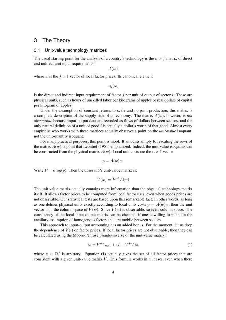
ation; the tangents to these isoquants (not shown) actually have the same slope as the economy-wide wage-rentals ratio. The unit value isoquants have curvature, and we are not depicting atechnology with fixed coefficients for good reason. The representative firm in every sector isminimizing costs by its choices of capital and labor, but the unit values in each sector may bemeasured with error by the econometrician.

The usual theoretical analysis would explain that the prices of the first and third goods haverisen and that of the second good has fallen; given the factor prices shown in the diagram, thesecond sector is not competitive, and it will shut down. Also the first and third sectors are makingpure economic rents, and those sectors will drive up local factor prices or drive down outputprices until the economy-wide zero-profit conditions in both remaining sectors are achieved.The general result is this: in an economy with f factors and n > f sectors, it will generally bethe case that only f sectors are actually active for an arbitrary specification of output prices p.Our data consist of unit-value matrices with n = 35 sectors and at most f = 4 factors in eachcountry.

Of course, in the data, almost every sector in every country actually produces positive output.In input-output data, one actually does see sectors that are shut down, where the relevant rowof the technology matrix consists of zeros. But this occurs at most in two or three of thirty-fivesectors for any country in our data. If the theory were completely correct, then this outcomewould be impossible (unless local prices satisfied very many over-identifying restrictions). Onthe other hand, this situation might occur if the econometrician is measuring the unit-valuematrix with error. Perhaps aggregation across firms in each industry introduces measurementerror. Perhaps different sectors have slightly different profit margins that are not recorded in unitinput costs. It might be the case that factors are not perfectly mobile across sectors, or factors arenot actually homogeneous. Indeed, capital or labor may be specific in many different sectors.

This measurement error has nothing to do with the observation of Melitz (2003) that efficientfirms tend to export. We are using the simple fact that aggregation schemes in macroeconomicaccounts record many more active sectors than factors of production. In fact, since we computerobust standard errors, we are quite agnostic about the sources of measurement error in thesetechnology matrices. But there can be no doubt that average factor use in each sector is mea-sured with error in the data that are typically used in computable general equilibrium models orempirical international trade.

3.3 Our Wald test

In this subsection, we show exactly how we conduct the Wald test for factor mobility and homo-geneity. Assume that the observed economy-wide factor prices w = (0.25, 0.25)T are consistentwith those in Figure 1, but the econometrician observes the data on factor use in Figure 2. Thepredicted unit costs for technology

V ′ =

2.9 0.92.2 2.20.9 2.9

7

L

K

1/w′1 = 4.02

1/w′2 = 4.021/p′3

1/p′2

1/p′1

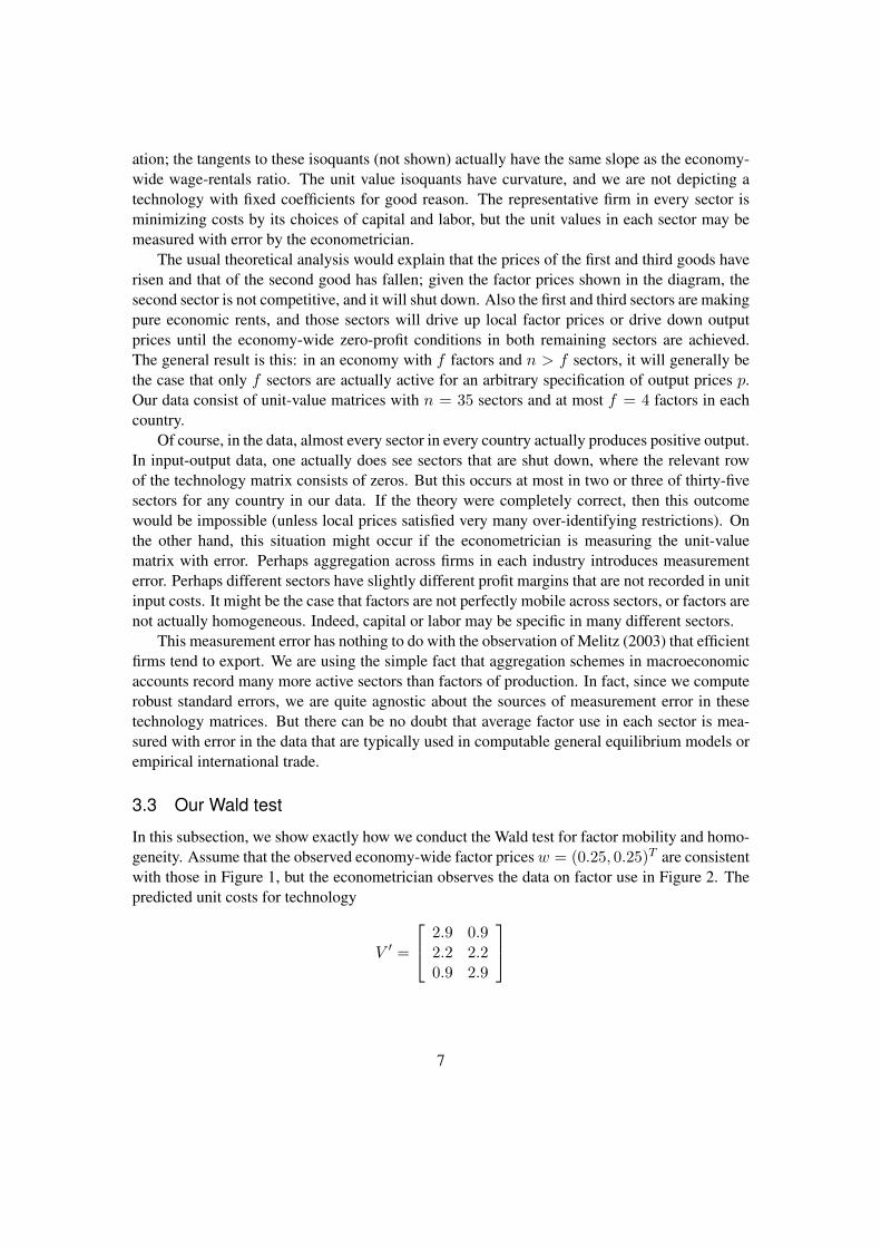
Figure 2: Three unit-value isoquants without a common tangency. Factor prices are the estimatedcoefficients from a regression of a vector of ones onto factor uses by sector.

are

p = V ′V ′+13×1 =

0.94531.09450.9453

.

The residual sum of squares is:

RSS1 = (p− 13×1)T (p− 13×1) = 0.0149

The predicted local unit costs under the restriction that w = (0.25, 0.25)T are:

p = V ′w =

0.951.10.95

and the restricted sum of squares is:

RSS2 = (p− 13×1)T (p− 13×1) = 0.015

8

Since the restricted sum of squares imposes f = 2 restrictions and the factor prices are estimatedfrom a regression with n− f = 3− 2 = 1 degree of freedom, the Wald test is constructed fromthe simple ratio:

F (f, n− f) =(RSS2 −RSS1)/f

RSS1/(n− f)=

(0.015− 0.0149)/2

0.0149/1= 0.0034. (3)

For a test of any reasonable size, one could not reject the null hypothesis that all factors weremobile, even though by inspection of Figure 2, the econometrician knows that the unit vectordoes not lie in the column space of V ′. In this case, the slight measurement error in V ′ is of nostatistical significance, and the maintained hypothesis of homogeneous factors earning identicalreturns in every sector is not rejected. Our actual tests use robust standard errors, so there isa slight modification to (3) using the estimated variance-covariance matrix from the regressionbased on (2).

Our null hypothesis is that factors are homogenous and mobile across sectors. Our alter-native hypothesis is that unit value isoquants may be so distant from the isocost line based onthe best estimate of common factor payments that random variations and measurement error areimplausible explanations. In other words, when we reject the null hypothesis we claim that itis more likely that factors earn distinct payments in different sectors, as would be predicted ina non-mobile world. However, we assess this variability with a carefully constructed statisticalhypothesis test and we have combined factors in a given industry in an economically meaningfulmanner.

4 The data

To implement our Wald test, we need to observe the unit value technology matrix and theeconomy-wide factor payments in a given country. The recently released World Input-OutputDatabase (WIOD) provides such data for forty countries, representing about seventy-five percentof world GDP.1 These countries include all the large developed economies and also major de-veloping economies such as China, India, and Indonesia. A novel feature of this database is thecombination of consistent input-output tables with extensive social and economic data includingthree types of labor and physical capital employed in thirty-five sectors.

We convert the input-output data into the unit value technology matrix in the followingfashion. First we construct an n × f matrix of direct factor usages. The units are hours ofunskilled labor per year, hours of middle skilled labor, hours of high skilled labor, and realdollars of capital. The skill category refers to levels of education where high skilled is tertiary orcollege education, medium school is secondary or high school education, and low skill is primaryor elementary school education. We consider several aggregations of these skill categories,described in greater detail later. Factor usage is recorded for 35 sectors encompassing 14 distinctmanufacturing sectors and a wide range of other goods and services sectors.

Intermediate goods flows between sectors are recorded in an n×n matrix whose typical ele-ment is dollars per year.2 Reading down a column, one sees dollars of different goods purchased

1See Timmer (2012) for complete details.2Conversions from local currency to US dollars are made with market exchange rates.

9

by an industry for its intermediate inputs. Reading across a row, one sees dollars of differentgoods sold to an industry. The row sums and column sums of these matrices must be equal,and an important part of national accounts is balancing these tables. The commodity flows arevalues; it is impossible to distinguish quantities from prices without further assumptions aboutthe data.

One must divide the elements of the commodity flow matrix by its column sums. Thisnormalization entails that one has now defined intermediate inputs per dollar of input in a sector.In particular, the commodity flow matrix now has no units. Its elements are scalars. The logicof Leontief’s algebra then allows one to calculate easily the infinite recursion of all the roundsof intermediate goods usages, and one inverts a simple matrix. Each element of this invertedmatrix again is a scalar.

Now comes the key step in defining a unit-value matrix. The direct factor uses are recordedin physical units of a factor per year. The input-output table’s column sums are dollars of outputper year. In constructing the Leontief matrix, one normalizes by these column sums. The samenormalization must be applied to direct factor uses. For example, one divides hours of lowskilled labor per year by dollars of output per year, and the resulting units are hours of lowskilled labor per dollar of output. This is a unit value. There is a nice subtlety; since directcapital input is measured in real dollars per year, its unit value is a scalar and should be properlyinterpreted as a gross rate of return.

The final step is to multiply the n × n Leontief matrix by the n × f matrix of unit values.This is how one constructs a consistent matrix V (w). One other minor comment is in order.Since one multiplies on the left by the square Leontief matrix, V (w) is linear in the columns ofthe direct factor use matrix. That means that it is completely consistent to aggregate hours oflow skilled labor per dollar of apple output with hours of middle skilled labor per dollar of appleoutput. In brief, our aggregation of labor into one broad category is economically sound.

We also construct the economy-wide payments for each factor in each country by dividingthe total value-added payments to that factor, reported in the WIOD, by the total factor usage ofthat factor. Figure 3 shows these observable factor payments in our sample countries, mappedagainst GDP per hour worked, also derived from WIOD values. Figure 3 shows the most aggre-gated verion of labor inputs, but we can easily disaggregate these labor payments into wages bythree educational categories.

We can also observe the variation of factor payments across 35 different sectors in each of the40 countries. We depict this variation for several large economies in Figures 4 and 5. Figure 4compares Germany to Spain, showing that in both countries there is noticeable variation in factorpayments. For example in both Germany and Spain, workers earn more than twice the averagewage in the petroleum refining sector and less than half the average wage in the agriculturesector. In both countries the return to capital is more variable across sectors than the averagewage. While the degree of variation by sector is again similar, Spain has an unusually high returnto capital in financial intermediation, reaching almost 4 times the average of all sectors. Figure5 depicts and compares the same variation in two large developing nations, China and India.

We present these detailed depictions of factor payments across sectors in these four countriesto highlight the level of detail the WIOD provides and the types of industries we observe. Tosummarize all 40 countries more succinctly, Figure 6 presents the coefficient of variation of the

10

average wage and return to capital. The coefficient of variation has been a standard measureof the degree of factor mobility in the literature, yet our wealth of data brings into focus thechallenge of using this single summary statistic to determine factor mobility. Looking at Figure6, there are certainly some countries with a higher coefficient of variation, but where would onedraw the line to separate countries with mobile factors (low coefficient of variation) from thosewith immobile factors (high coefficient of variation)? Likewise, how should one treat the twodistinct factors of capital and labor, when clearly capital has a higher coefficient of variationacross all countries? Rather than make arbitrary cut-offs for each factor, our approach brings theproduction economics of the Lerner diagram together with a straight-forward statistical test ofsignificance, allowing us to apply a uniform analysis to this diverse group of countries.

5 The results

Our Wald test is based on a comparison of the observable factor payments to the predictedpayments from the estimated coefficients in a regression of a vector of ones onto factor usesby sector as recorded in the technology matrix V . Our first test focuses on two factors, capitaland labor, for the year 2005. We show that for 24 of 40 countries, the null hypothesis of factormobility cannot be rejected. We then discuss the wage premium for college-educated workersand consider how more refined measures of labor perform in our mobility tests. Finally, wecompare the economic features of the countries whose factors are immobile to those countrieswhose factors are mobile.

5.1 Two factor mobility

Figure 7 depicts the results of our first test with aggregated labor and capital. Since our samplecountries have very different payment magnitudes, we present the ratio of the observed averagewage and the ratio of the observed rental rate to our estimated wage and rental rate. We are ableto accept the null hypothesis of factor mobility for 24 countries.3 As indicated in the figure,countries for which the null hypothesis is rejected fall roughly equally into two camps: thosewhose observed wage is above our estimates and those whose observed rental rate is above ourestimate.4

We present the standard statistical results of each of the 40 regressions in the data appendix.Almost all of the coefficients are statistically significant and greater than zero. Even for thosecountries for which we reject the null hypothesis of factor mobility, the coefficients of theseregressions offer a useful proxy for the economy-wide opportunity cost of labor and capital, afacet of our analysis that we explore later.

Many of the important issues relating to trade and factor mobility hinge on more refinedmeasures of skilled and unskilled labor. For example, do cheap clothing imports reduce the

3The countries with two mobile factors are Australia, Austria, Brazil, Canada, China, Denmark, Estonia, Fin-land, France, Germany, Greece, Hungary, Japan, Korea, Lithuania, Netherlands, Poland, Portugal, Romania, Russia,Slovenia, Sweden,Turkey, and the USA.

4The countries with immobile factors are Belgium, Bulgaria,the Czech Republic, India, Indonesia, Ireland, Italy,Latvia, Malta, Mexico, The Slovak Republic, Spain, Taiwan, and the United Kingdom.

11

wages of all unskilled workers or only those in the clothing industry? The considerable chal-lenge to this line of inquiry lies in accurately measuring labor skills across industries and, forinternational comparisons, across countries. Before considering disaggregated labor tests, wewould like to emphasize that our two factor test is not invalidated by unobserved differences inlabor quality. Even if we cannot separate different skill types, we are basing our estimated wageon the sum of labor inputs of all skill types captured in the respective column of the technologymatrix V . By way of contrast, it is easy to demonstrate that the coefficient of variation of averagewages across sectors will increase if the unobserved skill premium increases, even if the moreskilled workers earn the same wage in different industries. Likewise, in our test the technologymatrix incorporates the inputs of both labor and capital so that we can combine both factors inan economically meaningful way. Figure 7 highlights this distinctive feature by showing the twofactors on the same axes.

5.2 Disaggregating worker skill levels

We now evaluate factor mobility for disaggregated skill categories based on educational attain-ment. We begin by describing the salient features of the WIOD educational data. The WIODreports worker hours by three levels of educational attainment: high (college-degree or above),medium (high school and vocational school), and low (elementary school and some high school).Of the three educational categories, the share of college-educated hours, shown in Panel (a) ofFigure 8, is the most strongly correlated with GDP per worker. The share of medium and loweducation varies idiosyncratically among countries at similar income levels. For example, Mex-ico and Turkey have a similar level of GDP per worker and both have about 12 percent of collegeeducated workers. However, Mexico has 40 percent medium educated workers while Turkey hasonly 20 percent.

Panel (b) of Figure 8 shows that the college wage premium is decisively higher in low incomecountries. Among very low income countries such as Indonesian and India, college educatedworkers earn four to five times as much as those with no college. Even in the countries with thelowest premium, Denmark and Sweden, college educated workers earn about 30 percent morethan non-college educated workers.

Our analysis of factor mobility among different educational levels depends on detailed in-dustry level statistics of these educational categories. The statisticians who compile the WIODsocio-economic accounts apply Herculean efforts to obtain a disaggregated picture of wages andeducational level by industry from a range of national sources, as detailed in Erumban et al.(2012). Even for those European countries included in the extensive EU-KLEMS database, agreat deal of extrapolation is involved. For example, the EU-KLEMS data report education andwage breakdowns for at most 14 sectors, so that further disaggregation to 35 industries simplyassumes the same portions and relative wages in the corresponding sub-sectors. For seven coun-tries, data on the educational composition by industry simply does not exist, so the statisticiansinstead apply the educational distribution from another country.5

An additional complication is whether the educational level is an accurate indicator for skill-5These seven countries are Bulgaria, Estonia, Lithuania, Latvia, Malta, and Roumania, for which the educational

breakdown of Portugal is applied, and Russia, for which the educational breakdown of the Czech Republic is applied.

12

based wage premia. Among labor economists focusing on the United States economy, the degreeof correspondence between educational level and the particular skills or occupations which dis-tinguish high earners from low earners has been subjected to detailed scrutiny. Kambourov &Manovskii (2009) finds that occupational category is a more accurate determinant of wages thaneither education or industry. This assumption is echoed by Autor & Dorn (2013) who correlateover 300 occupational categories to a smaller set of skills including abstract, manual and rou-tine, skills. Among many of the developing countries in our sample, Pritchett (2013) raises avery different consideration. He documents extensively how the quality of education in manydeveloping countries is so poor that it may not even lead to literacy, let alone marketable jobskills.

With these caveats in mind, we first apply our Wald test to the most disaggregated measureof labor together with capital. At this detailed level of disaggregation, we can accept the nullhypothesis for 13 countries, all but two of which also show factor mobility when measured byaggregate labor. While these results seem reasonable, the coefficient estimates of the individ-ual types of labor are widely dispersed and often negative. However, if we combine low andmedium levels of education and conduct the test for 3 factors including capital, our coefficientsare generally well-behaved and we can accept the null hypothesis for 19 countries, all of whichalso show factor mobility with aggregate labor. We present the results of the 3 factor test inFigure 9.

The 5 countries which show mobility for aggregate labor and capital but not for either versionof disaggregated labor are Brazil, Japan, Portugal, Russia, and the United States. There are atleast two contributing factors to this outcome: the relatively poor quality of educational data byindustry, especially for Russia to which a proxy country was applied, and the poor correlationof labor skills with educational level. Of course the United States is of particular interest as theworld’s largest industrial economy. Since the United States is also one of the most accuratelymeasured economies in the world, we hope that our method can form the foundation for a moredetailed case study using different breakdowns of skills such those described in Autor & Dorn(2013).

5.3 Countries whose factors are immobile in 2005

We have identified 16 countries for which factors are immobile in 2005. For all of these coun-tries, we can reject the null hypothesis of factor mobility at both the 2 factor (labor and capital)and 3 factor level (college educated, non-college educated labor and capital). In the 2 factor case,our regression analysis provides an estimate of the average wage (w) and return to capital (r)that comes closest to equating unit costs of production in each sector to the unit price (assumedto be one dollar in all sectors). We can interpret these estimates as proxies for the economy-wideopportunity cost of labor and capital. This interpretation allows us to assess the magnitude ofthe distortions resulting from factor immobility.6

Let TL represent the observed total payments to labor in a given country, and TK representthe observed total payments to capital, and let K represent the total stock of capital and L the

6Since the sources of factor immobility are many, lumping together sector-specific human capital with regulatorybarriers to entry, we recognize that at least some of this measure may reflect healthy market forces.

13

total hours of labor employed. Our measure of the excess (deficit) payment to labor is givenby TL − wL and the excess (deficit) payment to capital is given by TK − rK. To compare themagnitudes among different countries, we normalize each excess factor payment by the totalpayment to that factor.

Figure 10 shows the results of this analysis for the 14 countries with immobile factors,compared to the 26 countries with mobile factors. The size of the distortion is substantial,representing on order of 50 percent of factor payments for countries with immobile factors.Although the number of countries is relatively small, there is considerable diversity in the sensethat nine of the countries have large excess payments to capital while seven have large excesspayments to labor.

6 Conclusion

Economists and political scientists alike have long been engaged in a debate about who benefitsand who looses from international trade. This debate often hinges on whether factors are mobilebetween industries, but what has been lacking is a statistically well-grounded measure of factormobility. We recognize that the solution we present in this paper demands a substantial amountof information on the technology of production in each country to which it is applied, but weshow that such information is necessary to discern whether or not the normal variability infactor payments across industries obscures an equilibrium consistent with factor mobility. Weshow that in a slim majority of countries, 24 out of 40, factors are mobile across sectors whenwe combine all educational levels of labor. In these countries, the evidence substantiates thestandard Heckscher-Ohlin results that trade has differential impacts on factor owners. Becauseour data encompass a detailed 35 industry structure over the entire economy, these results alsosubstantiate broader claims about labor market outcomes, such as Baumol’s well-known cost-disease argument.

In 16 countries our two factor test confirms that factors are immobile. The aggregate ef-fects of this immobility are substantial, typically representing around 50 percent of total factorpayments. This finding in turn justifies the interest of political scientists in the type of politicalcoalitions that might contribute to industry-specific protections. While we do not explore the po-litical dimensions of the economic outcomes we observe, we hope that our empirical test resultswill contribute to a better understanding of factor mobility and its implications for trade policyin both the economic and political realms.

Our approach is readily applicable to more refined measures of factor inputs by sector, andthe results of our test with skilled labor measured by college education is broadly consistent withour two factor tests. Of the 24 countries with two factor mobility, we confirm that 19 countriesexhibit factor mobility for skilled (college-educated) and unskilled labor and capital. However,we cannot confirm this finding for five countries including the U.S. and Russia. While this paperhas focused on a large international comparison in one year, our framework is readily applicableto more detailed case studies that can explore different measures of labor skills and evaluatechanges in mobility over time.

14

Table A1: SectorsNo. ISIC Rev. 3 Description1 A,B Agriculture, hunting, forestry and fishing2 C Mining and quarrying3 15,16 Food, beverages, and tobacco4 17,18 Textiles, textile products, leather and footwear5 19 Leather and footwear6 20 Wood and products of wood and cork7 21,22 Pulp, paper, paper products, printing and publishing8 23 Coke, refined petroleum products and nuclear fuel9 24 Chemicals and chemical products10 25 Rubber & plastics11 26 Other non-metallic mineral products12 27,28 Basic metals and fabricated metal13 29 Machinery, Nec14 30-33 Electrical and optical equipment15 34,35 Transport equipment16 36,37 Manufacturing, Nec; Recycling17 E Electricity, gas, and water supply18 F Construction19 50 Sale, maintenance and repair of motor vehicles; Retail sale of fuel20 51 Wholesale trade21 52 Retail trade22 H Hotels and restaurants23 60 Inland transport24 61 Water transport25 62 Air transport26 63 Other transport activities27 64 Post and telecommunications28 J Financial intermediation29 70 Real estate activities30 71-74 Renting of machinery & equipment and other business activities31 L Public administration and defense32 M Education33 N Health and social work34 O Other community, social and personal services35 P Private households with employed persons

15

Table A2: CountriesName Abbreviation GDP per hour workedAustralia AUS $39.04Austria AUT $43.66Belgium BEL $59.23Brazil BRA $4.30Bulgaria BGR $4.31Canada CAN $38.48China CHN $1.55Cyprus CYP $22.97Czech Republic CZE $12.35Denmark DNK $47.71Estonia EST $10.94Finland FIN $44.93France FRA $54.73Germany DEU $54.92Greece GRC $23.85Hungary HUN $12.41India IND $1.91Indonesia IDN $0.75Ireland IRL $51.63Italy ITA $38.12Japan JPN $39.23Korea KOR $15.07Latvia LVA $9.54Lithuania LTU $8.93Luxembourg LUX $70.93Malta MLT $19.23Mexico MEX $8.72Netherlands NLD $53.05Poland POL $11.19Portugal PRT $18.48Romania ROU $5.45Russia RUS $4.69Slovak Republic SVK $12.63Slovenia SVN $20.23Spain ESP $33.48Sweden SWE $50.14Turkey TUR $10.71United Kingdom GBR $45.44United States USA $47.42

16

Figure 3: Observable rate of return to capital and average hourly wage in 2005 for forty countries

17

(a) Return to capital

(b) Average wage

Figure 4: A comparison of factor payments across sectors in Germany and Spain in 2005

18

(a) Return to capital

(b) Average wage

Figure 5: A comparison of factor payments across sectors in China and India in 2005

19

Figure 6: The coefficient of variation in wages and return to capital in 2005 for 40 countries

20

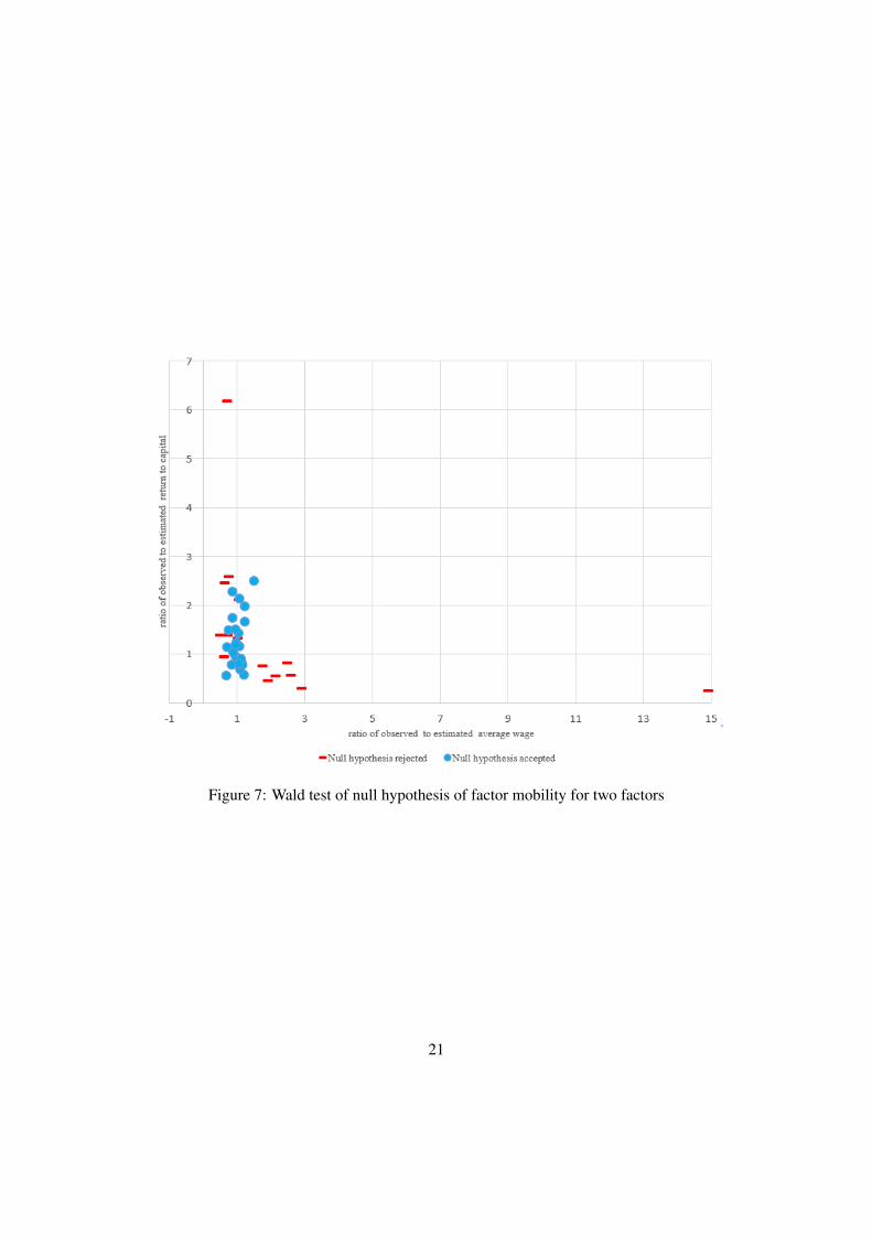
Figure 7: Wald test of null hypothesis of factor mobility for two factors

21

(a) College-educated worker hours, percent of total

(b) College wage premium

Figure 8: Share and earnings of college-educated workers in 2005

Note: College wage premium is the log of the ratio of the average hourly wage of college-educated workers to non-college educated workers.

22

(a) College wage and return to capital

(b) High school and below wage and return to capital

Figure 9: Wald test of null hypothesis of factor mobility for three factors

23

Figure 10: A comparison of select countries whose factors are mobile to those whose factors areimmobile in 2005

Note: The “immobility ratio” compares direct inputs (capital and labor) at sector-specific fac-tor payments to the hypothetical unit costs if factors had earned the observed economy-widepayments.

24

Bibliography

Autor, D. H. & Dorn, D. (2013), ‘The growth of low-skill service jobs and the polarization ofthe US labor market’, American Economic Review 103(5), 1553–1597.

Baumol, W. J. (1967), ‘Macroeconmics of unbalanced growth: The anatomy of urban crisis’,The American Economic Review 57(3), 415–426.

Baumol, W. J. & Ferranti, D. d. (2012), The Cost Disease: Why Computers Get Cheaper andHealth Care Doesn’t, Yale University Press, New Haven.

Cappelli, P. (2014), ‘Skill gaps, skill shortages and skill mismatches: Evidence for the US’.

Dickens, W. T. & Katz, L. F. (1987), Inter-industry wage differentials and industry character-istics, in K. Lang & J. Leonard, eds, ‘Unemployment and the Structure of Labor Markets’,Basil Blackwell Inc., Oxford.

Erumban, A., Gouma, R., de Vries, G., de Vries, K. & Timmer, M. (2012), ‘WIOD socio-economic accounts (SEA): Sources and methods’, Seventh Framework Programme .

Fisher, E. O. & Marshall, K. G. (2011), ‘The structure of the American economy’, Review ofInternational Economics 19(1), 15–31.

Gittleman, M. & Wolff, E. N. (1993), ‘International comparisons of inter-industry wage differ-entials’, Review of Income and Wealth 39(3), 295–312.

Grossman, G. M. & Helpman, E. (1994), ‘Protection for sale’, The American Economic Review84(4), 833–850.

Hiscox, M. J. (2001), ‘Class versus industry cleavages: Inter-industry factor mobility and thepolitics of trade’, International Organization 55(1), 1–46.

Hiscox, M. J. (2002), ‘Interindustry factor mobility and technological change: Evidence on wageand profit dispersion across U.S. industries, 1820-1990’, The Journal of Economic History62(02), 383–416.

Hwang, W. & Lee, H. (2014), ‘Globalization, factor mobility, partisanship, and compensationpolicies’, International Studies Quarterly 58(1), 92–105.

Jones, R. W. (1971), A three factor model in trade, theory, and history, in J. Bhagwati, R. Jones &R. A. Mundell, eds, ‘Trade, Balance of Payments, and Growth’, North-Holland, Amsterdam,pp. 3–12.

Kambourov, G. & Manovskii, I. (2009), ‘Occupational specificity of human capital’, Interna-tional Economic Review 50(1), 63–115.

Ladewig, J. W. (2006), ‘Domestic influences on international trade policy: Factor mobility inthe United States, 1963 to 1992’, International Organization 60(1), 69–103.

25

Leontief, W. (1951), The Structure of the American Economy, 1919-1939: An Empirical Appli-cation of Equilibrium Analysis, Oxford University Press, Oxford.

Lerner, A. P. (1952), ‘Factor prices and international trade’, Economica 19(73), pp. 1–15.

Melitz, M. J. (2003), ‘The impact of trade on intra-industry reallocations and aggregate industryproductivity’, Econometrica 71(6), 1695–1725.

Nordhaus, W. D. (2008), ‘Baumol’s diseases: A macroeconomic perspective’, The B.E. Journalof Macroeconomics 8(1).

Pennock, A. (2014), ‘The political economy of domestic labor mobility: Specific factors,landowners, and education’, Economics & Politics 26(1), 38–55.

Pritchett, L. (2013), The Rebirth of Education: Schooling Ain’t Learning, Center for GlobalDevelopment, Washington, D.C.

Rogowski, R. (1990), Commerce and Coalitions: How Trade Affects Domestic Political Align-ments, Princeton University Press, Princeton, N.J.

Samuelson, P. (1971), ‘Ohlin was right’, Swedish Journal of Economics 76(4), 35–84.

Timmer, M. P. (2012), The world input-output database (WIOD): Contents, sources and meth-ods, Technical Report Working Paper Number: 10.

26