Embed Size (px)
Citation preview

INTERNATIONAL JOURNAL FOR NUMERICAL METHODS IN ENGINEERINGInt. J. Numer. Meth. Engng 2015; 102:1784–1814Published online 9 January 2015 in Wiley Online Library (wileyonlinelibrary.com). DOI: 10.1002/nme.4865
A new sparse matrix vector multiplication graphics processing unitalgorithm designed for finite element problems
J. Wong, E. Kuhl and E. Darve*,†
Department of Mechanical Engineering, Stanford University, 496 Lomita Mall, Durand Rm 226, Stanford,CA 94305, USA
SUMMARY
Recently, graphics processing units (GPUs) have been increasingly leveraged in a variety of scientificcomputing applications. However, architectural differences between CPUs and GPUs necessitate the devel-opment of algorithms that take advantage of GPU hardware. As sparse matrix vector (SPMV) multiplicationoperations are commonly used in finite element analysis, a new SPMV algorithm and several variations aredeveloped for unstructured finite element meshes on GPUs. The effective bandwidth of current GPU algo-rithms and the newly proposed algorithms are measured and analyzed for 15 sparse matrices of varying sizesand varying sparsity structures. The effects of optimization and differences between the new GPU algorithmand its variants are then subsequently studied. Lastly, both new and current SPMV GPU algorithms are uti-lized in the GPU CG solver in GPU finite element simulations of the heart. These results are then comparedagainst parallel PETSc finite element implementation results. The effective bandwidth tests indicate that thenew algorithms compare very favorably with current algorithms for a wide variety of sparse matrices and canyield very notable benefits. GPU finite element simulation results demonstrate the benefit of using GPUs forfinite element analysis and also show that the proposed algorithms can yield speedup factors up to 12-foldfor real finite element applications. Copyright © 2015 John Wiley & Sons, Ltd.
Received 22 October 2013; Revised 18 July 2014; Accepted 7 December 2014
KEY WORDS: biomechanics; finite element methods; linear solvers; parallelization
1. INTRODUCTION
The recent use of graphics processing units (GPUs) for scientific applications has opened up pos-sibilities in achieving real-time simulations and has been shown to provide remarkable speedupfactors for many different applications. Scientific applications using GPUs range from computingthe flow over hypersonic vehicles [1] to finite element simulations of virtual hearts [2] and of vis-coelastic properties of soft tissue [3] to medical applications [4–6]. There is a developing body ofliterature concerning GPU implementation of finite element analysis codes.
Early papers investigating the use of GPUs for scientific computing focused on conjugate gradi-ent (CG) and multigrid solvers [7–9]. Several studies in the area of finite element method (FEM)have focused on the solution of the sparse linear system of equations Ax D b resulting from aFEM discretization [10–12], mainly because the solution stage is often the most computationallyintensive step. Some assembly strategies for the GPU have been mentioned as well. Often, specificapplications have allowed special approaches for FEM assembly. The methods described in [12]for geometric flow on an unstructured mesh and in [13] for FEM cloth simulation derive relatively
*Correspondence to: E. Darve, Department of Mechanical Engineering, Stanford University, 496 Lomita Mall, DurandRm 226, Stanford, CA 94305, USA.
†E-mail: [email protected]
Copyright © 2015 John Wiley & Sons, Ltd.

A NEW SPARSE MATRIX VECTOR MULTIPLICATION GPU ALGORITHM 1785
simple expressions for each non-zero in the system of equations. The relative simplicity and theinherent parallelism of computing each non-zero independently make these approaches well suitedfor GPUs. The PhD thesis of Göddeke [14] has an extensive discussion of the history behind GPUcomputing and the application of multigrid to FEM and its optimization for GPUs. Applications tothe FEM package FEAST [15] are discussed in [14].
Formulations have been considered in connection with discontinuous Galerkin methods. See [16]where the method is applied to Maxwell’s equations. For high-order, continuous Galerkin meth-ods, an assembly strategy is proposed in [17, 18]. Other successful approaches, such as [19] fordeformable body simulation, took advantage of vertex and fragment shaders on the GPU to per-form the assembly. New hardware and a more general computing environment appear to have madesome of these techniques obsolete. Markall et al. [20] compare FEM implementations on CPUs andGPUs. This paper includes a discussion of FEM along with spectral element methods and low-orderdiscontinuous Galerkin methods. Recent investigations include [21–24].
The difficulty in optimizing FEM calculations for GPUs has led some groups to develop spe-cial purpose languages and compilers to automate part of the process and separate the task ofimplementing novel numerical methods from the task of optimizing the computer implementation.Markall et al. [25] discusses the Unified Form Language for this purpose.
While GPUs are already used for many inherently parallel operations, such as material pointODE solvers for finite elements [26, 27] and for finite differences [28], total performance gains forfinite elements on GPUs can only be realized by efficiently combining all aspects of the calculation:element calculations, global assembly, and solver.
In this work, one of the focuses is the sparse matrix solver that is used as part of FEM. How-ever, it is generally not possible to simply ‘port’ CPU algorithms to the GPU. Typically, suchimplementations result in a GPU code that may be slower than the CPU code. Differences in GPUmemory architecture, speed of individual GPU cores, and the communication between GPU cores,GPU memory, and host (CPU) memory can greatly impact the performance of GPU algorithms.Because of these differences, much effort has been spent in developing new algorithms designed forgeneral-purpose use.
The performance of many of these algorithms is dependent on the structure of the data. In partic-ular, sparse matrices can be represented by a variety of formats, and the computational performancemay differ greatly depending on the format used [29]. There is a large body of literature on theinvestigation of various formats and their efficiency.
A sparse matrix contains mostly null entries. As a result it is advantageous to store only the non-zero entries along with their location in the matrix. The difficulty with such a storage is that it leadsto a random access to memory, such that the performance is heavily limited by memory bandwidthand often very low. As a result, several storage schemes attempt to make the memory access muchmore regular such that the effective memory bandwidth increases. This is crucial on GPUs wherecoalesced [30] memory access (i.e., accessing a 128-byte aligned segment in the device memory)is crucial for best performance. The study of Bell et al. [29, 31] was an early paper on SMPV anddiscusses all the key sparse matrix formats including the diagonal format (DIA); ELLPACK, inwhich all non-zero entries are stored in an N � K dense matrix (N is the number of rows in thematrix and K the maximum number of non-zeros per row); the coordinate format (COO, with asimple row, col, and data format); compressed sparse row (CSR) format (this is a popular formaton CPUs); and the hybrid format that combines ELLPACK with COO. At the end of the paper, thepacket format (PKT) is discussed. In this format, the matrix is decomposed into blocks with a highdensity of non-zero entries, and a type of ‘local’ CSR format is used to store entries associated witheach block (offsets from the base index are stored using 16-bit integers).
Before exploring in more details various papers that followed the footsteps of Bell, we mentionthe CUSP library [32] by Bell and Dalton, which implements various matrix formats and itera-tive schemes. cuSPARSE [33] is a library released by NVIDIA, which contains code for SPMV,sparse matrix-matrix addition and multiplication, sparse triangular solve, a tri-diagonal solver, andincomplete factorization preconditioners.
Among the newer implementations, we start with a series of papers on variants of the ELLPACKformat. ELLPACK-R [34] uses an ELLPACK format, and each thread computes a single row. An
Copyright © 2015 John Wiley & Sons, Ltd. Int. J. Numer. Meth. Engng 2015; 102:1784–1814DOI: 10.1002/nme

1786 J. WONG, E. KUHL AND E. DARVE
additional array is used to store information about the true number of non-zero elements per row (notaccounting for the ELLPACK padding), such that each thread is not required to do more floating-point operations than strictly necessary. This reduces the number of extra flops usually found inELLPACK. Vazquez et al. [35] revised his original algorithm and renamed it ELLR-T in 2010. Inthis work, he uses T threads to compute a single row in SPMV. The Sliced ELLPACK [36] formatis similar to ELLPACK. However, it is more flexible and uses a storage scheme that varies thenumber of non-zero entries stored across CUDA warps. This amounts to an ELLPACK where K isa function of the warp index or slice. The Sliced ELLPACK and ELLR-T (many threads per row)ideas are combined in the Sliced ELLR-T scheme of Dziekonski et al. [37].
A series of papers considered the block CSR (BCSR) format. BCSR stores the non-zero entriesas a sequence of fixed-size r � c dense blocks. BCSR uses one integer index of storage per blockinstead of one per non-zero as in CSR, reducing the index storage by 1=.rc/. Moreover, fixed-sizedblocks enable unrolling and register-level tiling of each block multiply. The speedup achieved isunfortunately mitigated by fill-in of explicit zeros resulting from this storage. Vuduc and Moon [38]mitigated these issues by splitting the matrix into a small set of matrices, each with its own .r; c/and using a more flexible storage scheme called unaligned BCSR. In [7], the BCSR scheme (calledin that paper BCRS—block compressed row storage) is used to implement a sparse general-purposelinear solver (i.e., Jacobi-preconditioned CG). Monakov and Avetisyan [39] explored a variant with ahybrid BCSR/BCOO format. BCSR uses a CSR-like format to store blocks. The column coordinatefor each block is stored, and the row coordinate is implicitly encoded by sorting blocks by rowsand then storing the index of the first block in each row in a CSR-like format. On the other hand,BCOO uses a blocked coordinate format where both coordinates of a block are stored. This providesadditional flexibility in comparison with a pure BCSR format.
We mention a separate line of research by Baxter [40]. In the ModernGPU library, Baxter consid-ers an SPMV as a sequence of two steps. Step 1 is comprised of element-by-element multiplicationof matrix entries by vector entries. This step is extremely parallelizable and runs near peak per-formance on GPUs. Step 2 is comprised of a segmented reduction (i.e., a large sequence of shortreductions) to produce the final output vector. The focus is therefore on implementing an effi-cient segmented reduction. The resulting algorithm has high efficiency but is also very complex toimplement and modify. The overall approach is very different compared with other SPMV papers.Nonetheless, it has produced some of the fastest SPMV GPU codes currently available.
Our new algorithm follows in the footsteps of the ‘padded jagged diagonals storage’ (pJDS)scheme [41]. This is one of the most efficient storage formats available. It reduces the memoryfootprint by up to 70% and achieves 95–130% of the ELLPACK-R performance. A main drawbackof ELLPACK-R and its sliced version is that when rows are highly inhomogeneous (the number ofnon-zeros varies significantly), memory and floating-point operations are wasted, and this overheadmay become notable. In contrast, pJDS sorts all the rows from longest to shortest. The rows are thengrouped into slices (as in sliced ELLPACK-R) and then packed with zeros up to the longest row.Because of the sorting, the extra padding is minimal, and most floating-point operations becomemore efficient. Here is the pseudo-code for this algorithm:
Copyright © 2015 John Wiley & Sons, Ltd. Int. J. Numer. Meth. Engng 2015; 102:1784–1814DOI: 10.1002/nme

A NEW SPARSE MATRIX VECTOR MULTIPLICATION GPU ALGORITHM 1787
The permutation on the rows of the matrix means that entries in the vector should be permutedas well. There is a computational cost associated with that. However, in the context of iterativemethods, this overhead is mitigated. The approach in this paper has a similar drawback.
In developing a GPU-based finite element code for real-time heart simulations, we developed avariant of pJDS. We found that it works very well for finite element unstructured grids as well asa variety of other sparse matrices as found in the benchmark suite of Williams et al. [42, 43]. Ouralgorithms take a novel approach by systematically addressing issues with current GPU algorithmsrelated to row length irregularity, padding efficiency of matrices, and data localization for GPUs.While other algorithms have similar insights in gaining additional performance for finite elementSPMV operations by grouping rows with the same row structure [38, 41], encoding sparse matricesin blocks [7, 36, 37], or utilizing data coalescing repacking algorithms [35, 40], our algorithms weredesigned to reduce GPU data locality issues, increase memory throughput, and perform well onrelatively unstructured meshes with a substantial degree of irregularity in row lengths distributions.
Compared with the pJDS scheme (row sorting) discussed earlier, our algorithm differs in a fewways. We use a warp optimized storage. As in pJDS, rows are grouped together into sets (slice)such that a single warp processes a given set. Inside a set, the number of non-zero entries is takento be constant and is set to be equal to the maximum exact number of non-zeros in the row set.Entries for a given set are stored contiguously in memory such that the memory access by threads isperfectly coalesced. A varying number of threads are assigned to a given row. This allows optimizingsituations in which few rows are significantly longer than others. In that case, a large number ofthreads (or all 32 threads in a warp) can be assigned to that row. As a result, per warp, we basicallyonly need to know three integers for memory access: the starting address in the matrixA, the numberof rows processed by the warp, and the number of non-zero entries per thread. Because of thepermutation on the rows of the matrix (as in pJDS), the sequence of column indices inside a givenrow is typically ‘random’. We sorted them in order to improve cache performance when accessingthe right-hand side vector x. In some sense, our algorithm combines insights from ELLPACK-R(varying the number of non-zeros K), sliced format (reduced storage), ELLR-T (many threads perrow; in our case, the number of threads per row is not even constant and is adjusted for load-balancing), and pJDS (sorting of rows). We called our new scheme ELL-WARP.
An algorithm called SELL-C -� was proposed in a recent paper submitted for publication andavailable via ArXiv [44]. This publication compares Intel, Intel Phi, and Nvidia architectures, andthey examine different metrics with which to evaluate their SELL-C -� algorithm. We developed ouralgorithms independently. Our algorithm K1 is equivalent to SELL-C -� . Their paper also highlightsdifficulties in addressing certain types of matrices. Some of these concerns are in fact addressed wellby our K2 algorithm. In contrast with [44], this paper concentrates on examining the GPU aspectsof the algorithm, important details regarding the necessary reordering costs of these classes of algo-rithms, and also proposes some techniques of ameliorating those issues. Lastly, while this paperconfirms some of the observations of the aforementioned paper, we also provide further insight intoother important aspects of SPMV computational performance differences by detailing the impact ofthe various optimizations considered in our GPU kernels.
We also note that within the context of the FEM, our novel SPMV routines can be leveragedboth for the global assembly operation and within the solver to gain additional computationalperformance.
In this paper, we first describe the computational heart simulation problem within the context of atraditional finite element framework. We then highlight computational costs for both the assemblerand solver and highlight differences between CPU and GPU implementations. A survey of differentGPU SPMV algorithms then follows. A new set of SPMV algorithms is introduced, and a variety ofSPMV algorithms are benchmarked against our novel algorithms. Different aspects of optimizationsused in the development of our algorithms are investigated. We discuss the utility of our SPMValgorithms in the contexts of finite elements and general computational settings. Lastly, we end withconcluding remarks where we highlight possible future improvements to our algorithms and alsodiscuss possible improvements in leveraging GPUs for finite element simulations.
Copyright © 2015 John Wiley & Sons, Ltd. Int. J. Numer. Meth. Engng 2015; 102:1784–1814DOI: 10.1002/nme
1788 J. WONG, E. KUHL AND E. DARVE
2. DESCRIPTION OF THE PHYSICAL PROBLEM
Our original aim was to utilize GPUs for achieving real-time electrophysiological simulations ofthe heart. The electrical propagation of voltage within the heart is described by the followingtwo-variable phenomenological governing differential equations for non-linear mono-domainexcitable tissues.
P� D div q.�/C f �.�; r/ (1)
Pr D f r.�; r/ (2)
The transmembrane voltage, �, is the voltage difference across the cell membrane, while thephenomenological variable, r , describes the recovery behavior of cardiac tissue. To account forconduction throughout the tissue, a phenomenological potential flux term div q is added.
q D D � r� (3)
A phenomenological diffusion tensor D D disoI C danin ˝ n allows for cell-to-cell electricalcoupling across cellular gap junctions. diso and dani are the respective isotropic and anisotropicconduction terms, and n is the preferred direction of anisotropic conduction.
In this paper, we will use the classical Aliev–Panfilov model [45] for convenience to evaluate theeffectiveness of our GPU algorithms. The source terms for the Aliev–Panfilov model are
f � D c � Œ� � ˛�Œ1 � �� � r � (4)
f r D
�� C
�1 r
�2 C �
�Œ�r � c � Œ� � b � 1�� (5)
While the mono-domain Equations (1) and (2) can be solved simultaneously, a global–local internalvariable splitting approach [46, 47] is taken because it yields a global symmetric tangent matrix forthe global degree of freedom, �, such that a fast iterative GPU solver can be effectively employed.In our splitting approach, we take the transmembrane voltage, �, to be our global variable and r tobe our local variable. r is local in the sense that the value of r at a given point in time is not directlyaffected by the current values at the neighboring points. r at a given point is affected by neighboringpoints through coupling through �.
An implicit semi-discretization approach is taken where backward Euler time integration is used,and the mesh is discretized spatially using Lagrangian shape functions. The heart mesh is discretizedin space using isoparametric tetrahedral elements in this paper using Equation (6). N is a tetrahe-dral shape function, while ı�i and �j are the respective test function local nodal values and localnodal solution values. Be is the domain of the element, and nen is the number of nodes within aparticular element.
ı�hjBe D
nenXiD1
N i ı�i �hjBe D
nenXjD1
N j �j (6)
After the initial spacial discretization has been performed, initial values are set for the global vari-ables, �J , at the finite element nodes, while the internal variable r is initialized at each integrationpoint within each element. As the coupled non-linear problem is stiff, backward Euler implicit timeintegration is used where �n denotes the fully converged solution at the previous timestep.
P� �1
�tŒ � � �n �
For a given timestep, n C 1, Newton’s method is applied over the finite element nodal values,�J , such that the global residual, R� is fulfilled. In order to ensure that the residual for the internalvariable, Rr , is also fulfilled over the whole domain, we apply Newton’s method at every integrationpoint within every element and update r such that Rr is fulfilled at every point. Therefore, the
Copyright © 2015 John Wiley & Sons, Ltd. Int. J. Numer. Meth. Engng 2015; 102:1784–1814DOI: 10.1002/nme

A NEW SPARSE MATRIX VECTOR MULTIPLICATION GPU ALGORITHM 1789
non-linear rate Equation (2) is first solved locally using Equation (7). The tangent matrix Kr andresidual Rr are constructed at each integration point and used to iteratively determine the convergednon-linear solution for the given timestep, nC 1.
Rr D Pr � f r.�; r/ Kr D drRr D
dRr
dr(7)
With r updated based on the �J values of the current time step and current Newton iteration, theterms for the global residual,R�I , can be calculated using Equation (8). The tangent term d�f �.�; r/necessary for computing R
� eI , the global residual contributions from each element, can be computed
in a straightforward manner, and the tangent term is used to obtain the completed global elementtangent matrix K� e
IJ for each element. The details for this procedure can be found in [47]. Theglobal element residuals R� e
I are then calculated and together with the element tangent matrices areassembled to form the global tangent matrix K�IJ and global residual vector R�I , as is performednormally in non-linear finite elements.
R� eI D
P�e � div q.�e/ � f �.�e; re/ K� eIJ D d�e
JR� eI D
dR� eI
d�eJ
(8)
With the global tangent matrix and residual, the global finite element problem is solved iterativelyusing Newton’s method over the domain. Both the local and global degrees of freedom are updatedat each global Newton–Raphson iteration to ensure the consistency of the solution. This process isrepeated until convergence is reached at each timestep.
The scheme is summarized in Table I.
Implicit time integration can be further leveraged by using adaptive time-stepping schemes tofurther reduce the computation time. Lastly reduced-order integration is used, whereby a lineartetrahedral element will only have one integration point. All implementations developed in this studyare scientifically accurate and run at double precision.
Table I. An algorithmic treatment of the transmembrane voltage in excitable cardiac tissue based on finiteelement discretization in space and implicit finite difference discretization in time embedded in two nested
Newton–Raphson iterations.
The electrical unknown, the membrane potential �, is introduced globally on the node point level, whereas thephenomenological recovery variable, r , is introduced locally on the integration point level. Element assembly is
highlighted in blue, and the solution update is highlighted in red.
Copyright © 2015 John Wiley & Sons, Ltd. Int. J. Numer. Meth. Engng 2015; 102:1784–1814DOI: 10.1002/nme
1790 J. WONG, E. KUHL AND E. DARVE
2.1. Computational cost of the finite element method
While the biophysical problem may initially seem rather specific, the problem has been structured inthe standard non-linear solid mechanics finite element framework. For example, such local–global
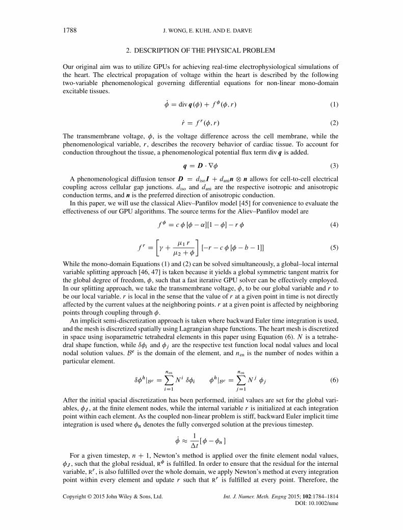
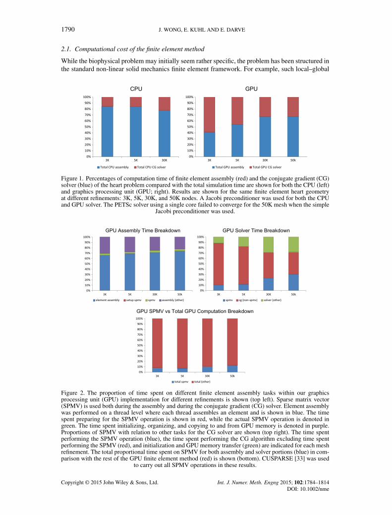
Figure 1. Percentages of computation time of finite element assembly (red) and the conjugate gradient (CG)solver (blue) of the heart problem compared with the total simulation time are shown for both the CPU (left)and graphics processing unit (GPU; right). Results are shown for the same finite element heart geometryat different refinements: 3K, 5K, 30K, and 50K nodes. A Jacobi preconditioner was used for both the CPUand GPU solver. The PETSc solver using a single core failed to converge for the 50K mesh when the simple
Jacobi preconditioner was used.
Figure 2. The proportion of time spent on different finite element assembly tasks within our graphicsprocessing unit (GPU) implementation for different refinements is shown (top left). Sparse matrix vector(SPMV) is used both during the assembly and during the conjugate gradient (CG) solver. Element assemblywas performed on a thread level where each thread assembles an element and is shown in blue. The timespent preparing for the SPMV operation is shown in red, while the actual SPMV operation is denoted ingreen. The time spent initializing, organizing, and copying to and from GPU memory is denoted in purple.Proportions of SPMV with relation to other tasks for the CG solver are shown (top right). The time spentperforming the SPMV operation (blue), the time spent performing the CG algorithm excluding time spentperforming the SPMV (red), and initialization and GPU memory transfer (green) are indicated for each meshrefinement. The total proportional time spent on SPMV for both assembly and solver portions (blue) in com-parison with the rest of the GPU finite element method (red) is shown (bottom). CUSPARSE [33] was used
to carry out all SPMV operations in these results.
Copyright © 2015 John Wiley & Sons, Ltd. Int. J. Numer. Meth. Engng 2015; 102:1784–1814DOI: 10.1002/nme

A NEW SPARSE MATRIX VECTOR MULTIPLICATION GPU ALGORITHM 1791
splitting schemes are commonly used in the field of plasticity [48]. A comparison between the com-putational cost of our heart simulation for various refinements of the same mesh is shown in Figure 1for a single CPU FEM implementation of the electrophysiological problem using a standard scien-tific code, PETSc [49], and for our custom single GPU implementation. A Jacobi preconditionerwas used for both the CPU and GPU solver. Four different mesh refinements were created havingroughly 3000 nodes, 5000 nodes, 30,000 nodes, and 50,000 nodes. These meshes have 11k, 16k,123k, and 218k elements, respectively.
Our GPU implementation utilizes SPMV multiplication operations to assemble the global tangentand residual quantities, and SPMV is also employed in our standard Jacobi preconditioned CGsolver. The use of SPMV within the context of CG solvers is prevalent [7–9, 38, 39]; however,the benefit in using SPMV for global assembly on GPUs is not particularly obvious and will beexplained in more detail in the following sections.
For our GPU heart simulations, the portion of time spent on SPMV during assembly is relativelysmall compared with the total assembly time and increases toward 33% within the CG solver as thelevel of refinement increases (Figure 2). Together, the total time spent in our GPU implementationshows that up to 10% of the computation time is spent purely on SPMV calculation. However, ifother parts of the code are further optimized and accelerated, it is possible that the SPMV calculationcould become a considerable bottleneck. Thus, while general finite element problems may exhibitdifferent solver-to-assembly ratios, improvements to SPMV operations can be beneficial to finiteelement frameworks. In the following sections, we will investigate various improvements and novelmodifications to current SPMV algorithms and highlight their use within the FEM and in othergeneral SPMV applications.
3. GRAPHICS PROCESSING UNIT ARCHITECTURAL ORGANIZATION
As GPUs are architecturally organized differently than traditional CPUs, a brief summary is givenbefore we examine current GPU algorithms. These architectural differences are important in devel-oping a substantially improved SPMV algorithm. Because we are using an Nvidia GPU, we willdescribe the general organization of an Nvidia GPU. The overall work-execution model on the GPUis composed of individual threads that each execute a specified kernel routine concurrently withrespect to other threads Single-Instruction Multiple-Thread (SIMT). Groups of 32 threads, calledwarps, are executed synchronously. Furthermore, up to 32 warps can be grouped into a block (CUDACompute Capability 2.0). Threads from a block have access to shared memory within that block andcan also be forced to synchronize with other threads within that block.
On the GPU, there are basically four types of memory available: global, shared, local, and registermemory. In general, memory that is available to more threads is slower than memory that is sharedwithin a smaller group of threads. For example, global memory can be accessed by all threads on aGPU, but it is also the slowest form of memory available. Shared memory is shared within a block. Itis always faster than global memory. However, memory bank conflicts may occur when threads areaccessing the same shared memory banks simultaneously. Local memory is global memory reservedfor threads where stores are kept in the L1 cache. Generally, its use is specified by the compiler,and it is used when a thread has fully utilized the maximum amount of memory registers available.Registers are the fastest form of memory, and only 63 registers are available for a given thread forthe GPU used in this work. Different memory caches are used to facilitate memory accesses to andfrom the different types of memory to the individual threads. In this paper, the L1 and L2 caches areimplicitly used, and use of the texture cache, which is a special spatial locality-based global memorycache, is also investigated.
4. DESCRIPTION OF CURRENT GRAPHICS PROCESSING UNIT METHODS
In order to achieve real-time finite element heart simulations, ideally both the finite element tangentmatrix assembly and finite element solver will perform a majority of the computations on the GPUto minimize CPU-to-GPU memory transfer overhead. Current GPU approaches and methods aresummarized in the succeeding text.
Copyright © 2015 John Wiley & Sons, Ltd. Int. J. Numer. Meth. Engng 2015; 102:1784–1814DOI: 10.1002/nme
1792 J. WONG, E. KUHL AND E. DARVE
For the finite element assembly of cardiac simulations, efforts have been made at leveragingGPUs to speed up the evaluation of the local ODE problem (2) [26, 27]. Because we have chosena simple phenomenological model, these efforts are not directly applicable to this study. However,several different finite element assembly approaches have been recently investigated [20, 21, 50, 51].In Cecka et al., it is shown that assembly by non-zeros of the finite element tangent matrix is abetter approach compared with assembly by elements, which is the traditional serial finite elementapproach. Furthermore, if we restructure the assembly such that shared memory is used instead ofglobal memory, further speedups are possible. However, this improvement requires a substantialrewrite of the FEM and is dependent on the particular type of element. The method of coloring,where elements are specified in a way such that threads can safely accumulate entries in the globalmatrix without potential race conditions, can also be used, but multiple passes are typically required,and memory traffic may increase. These consequences may affect the overall performance; however,the number of flops is often nearly optimal. Also of note, in Markall et al. [20], a method (similarto ours) for assembly of the residual vector is proposed. In their case, however, they do not actuallyassemble the matrix. Instead, they compute and store the elemental contributions and use those in amatrix-free manner to calculate K� �x D R� .
Much work has also been carried out on finite element CG solvers and multigrid solvers on GPUs[2, 7, 9, 38]. Lastly, both the finite element assembly on the GPU and CG method utilize forms ofSPMV product multiplications.
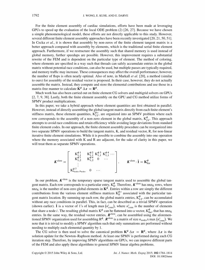
In this paper, we take a hybrid approach where element quantities are first obtained in parallel.However, instead of directly assembling the global tangent matrix directly from each finite element’sstiffness matrix, these element quantities, K� e
IJ , are organized into an SPMV problem where eachrow corresponds to the assembly of a non-zero element in the global matrix, K�IJ . This approachattempts to avoid race conditions and retain efficiency while avoiding large deviations from standardfinite element codes. In our approach, the finite element assembly procedure can be reorganized intotwo separate SPMV operations to build the tangent matrix, K, and residual vector, R, for non-lineariterative finite element simulations. While it is possible to combine the assembly into one operationwhere the memory associated with K and R are adjacent, for the sake of clarity in this paper, wewill treat them as separate SPMV operations.
K elem D
266664
K� 11;1 K� 21;1 K� 31;1 K� 41;1 � � �
K� 11;2 K� 41;2 0 � � �:::
K� 7nnodes;nnodes 0 � � �
377775 ; K elem � N1 D K�
flat
In our problem, K elem is the temporary sparse tangent matrix used to assemble the global tan-gent matrix. Each row corresponds to a particular entry, K�IJ. Therefore,K elem has nnzK rows, wherennzK is the number of non-zero global elements in K� . Entries within a row are simply the differentcontributions from the various element stiffness matrices K� e
IJ associated with the particular tan-gent matrix location. By summing up each row, the global matrix entries, K�IJ , can be accumulatedwithout any race conditions in parallel. This, in fact, can be described as a trivial SPMV operation(shown earlier). N1 is a vector of 1’s of length max
�ni
conn
�, where ni
conn is the number of elementsthat share a node i . The resulting global matrix K� can be flattened into a vector, K�flat, that has nnzK
entries. In the same way, the residual vector entries, Relem, can be assembled using the aforemen-tioned SPMV organization used for assembling R� .Relem is a matrix of size nnodesx max
�ni
conn
�. We
note that it is trivial to modify a SPMV algorithm such that only summations are performed withoutneeding to multiply each elemental quantity by 1.
The CG solver is then used to solve the canonical problem K� �x D R� , where �x is thesolution update for the Newton–Raphson method. At least one SPMV is performed during each CGiteration step. Therefore, by improving SPMV algorithms on GPUs, we can improve different partsof the FEM and also apply these algorithms to general SPMV linear algebra problems.
Copyright © 2015 John Wiley & Sons, Ltd. Int. J. Numer. Meth. Engng 2015; 102:1784–1814DOI: 10.1002/nme

A NEW SPARSE MATRIX VECTOR MULTIPLICATION GPU ALGORITHM 1793
While there are many variations of SPMV product GPU algorithms [7, 38, 39], the majority canbe summarized by the available implementations from several commonly available SPMV libraries:CUSPARSE [33], CUSP-library [32], and ModernGPU [40]. In [29], COO, CSR, ELL, and HYBformats are examined and analyzed. A review of the different formats and algorithms is highlightedin the succeeding text. In this section, we will look at the classical SPMV problemAx D y , wherex is given and the objective is to calculate the vector y .
4.1. COO
The coordinate list (COO) sparse matrix format is composed of three array lists of row indices,column indices, and the corresponding list of matrix values. In the CUSP COO implementation,row indices are sorted in order. Each warp processes a section of the matrix and works over 32 non-zero values at a time. Each thread within the warp performs a multiplication between the thread’svalue and the corresponding value from the vector. The different row segments are summed usingsegmented reduction, which is a method of efficiently distributing the reduction over a warp evenif the warp is computing the sum for different rows. During the initial stage, the product is storedin shared memory, and intra-warp segmented reduction is performed on the element products. Thefirst thread within each warp determines whether to include results from previous warp iteration inits row sum and, if not, updates the solution vector. Intra-block segmented reduction is then used toproperly accumulate rows that span multiple warps.
COO SPMV algorithms generally suffer from poor memory to computation ratios as row, andcolumn indices must be retrieved for each computation. Row indices are also required for row sumreduction, and additional explicit intra-block thread synchronization may be required depending ifrows span multiple warps.
4.2. Compressed sparse row
The CSR matrix storage format is composed of three array lists of values, corresponding columnindices, and corresponding row offsets that index the beginning of each row in the arrays of values.In the CUSP CSR vector implementation, a warp is assigned to each row in the matrix. A warpprocesses a continuous section of values and corresponding column indices in a coalesced manner.Intra-warp reduction is performed, and sums are accumulated in the solution vector.
The main issue with CSR algorithms is that while the storage is space efficient and the memoryaccess pattern is contiguous, memory accesses are not aligned. The CUSP implementation will alsosuffer when the size of a row is less than the warp size. However, unlike an alternative CSR algorithmwhere each thread is assigned to a row, the access pattern in CUSP is coalesced and contiguous.
4.3. ELL and ELL variants
In the ELLPACK (ELL) format, the matrix is again described by two array lists of values andcolumn indices. The maximum size of the longest row in the matrix is allocated for each row in theELL format. Non-zero values are ordered contiguously, and the remaining values are typically zeropadded. Column indices are arranged and padded in a similar manner. Both values and columns arestored in column-major order. The GPU kernel is fairly simple. Each thread is responsible for a row,and matrix vector products are summed in a coalesced manner.
The ELL format performs poorly when the row size varies from row to row resulting in poor workdistribution within each warp. The format also suffers from issues with excess padding when thelongest and shortest rows differ greatly in length and when the average row length is significantlyshorter than the longest row.
There are several variations of the ELL format, which attempt to fix these issues. One is theELL-R format [34] where an extra vector is provided that designates the number of non-zeros eachrow is responsible for. Another is Sliced ELLPACK [36] where the matrix is sliced into groups ofconsecutive rows and then stored in the ELLPACK format. The ELLR-T [35] and sliced ELLR-Tformats [37] use multiple threads per row. Lastly, another variant is the pJDS format [41], which is
Copyright © 2015 John Wiley & Sons, Ltd. Int. J. Numer. Meth. Engng 2015; 102:1784–1814DOI: 10.1002/nme

1794 J. WONG, E. KUHL AND E. DARVE
similar to ELL-R. In this format, the rows are first sorted from the longest to shortest row and thensliced and padded in a manner similar to the ELL-R format.
4.4. HYB
The Hybrid format is similar to the ELL format. To reduce the amount of zero padding due to row-to-row size differences, a certain number of values, determined empirically, are stored in ELL, andthe remaining entries are stored in COO format. The CUSP implementation is simply a combinationof the ELL kernel and the COO kernel.
Because of the more efficient storage scheme, the hybrid format requires launching of two kernelsin order to perform the sum. While the values of the matrix are contiguous in each kernel, the accesspattern for the vector will generally not be so.
4.5. Modern graphics processing unit
ModernGPU takes a different approach with its SPMV implementation called mgpusparse (MGPU).The algorithm is somewhat complicated but is essentially constructed to address several issues withthe aforementioned algorithms. It is a combination of a series of parallel and segmented scans. Dataare partitioned into the list of values, list of corresponding column indices, and several lists are usedto keep track of the ends of rows and row segments. Data are also arranged in a coalesced way similarto column-major storage but for fixed-sized chunks of matrix values. Two kernels are utilized. In thefirst kernel, each thread within a warp is responsible for calculating valuesPerThread partialrow sum entries. A serial scan is performed by each thread, and the sums of different row segmentsare stored in shared memory. A number of flags are associated with each thread, such that eachthread can determine where to store the partial sum for a given row segment in shared memory.An intra-warp parallel scan is then performed to reduce rows within each chunk quickly. Lastly, anintra-block segmented reduction is performed to reduce rows that span multiple blocks.
MGPU also takes advantage of index representation compression and performs other compres-sion tricks to increase efficiency. The algorithm generally performs well in comparison with theaforementioned algorithms. The main drawback, however, is the complexity of the algorithm andthe amount of book-keeping that is necessary. The main benefits are that the workload for threadswithin a block is very well distributed, and very few threads are idle compared with the rest of thethreads within each block.
5. DEVELOPMENT OF NOVEL GRAPHICS PROCESSING UNIT ALGORITHMS
There are several other variations of the previously mentioned algorithms. Most variations concen-trate on increasing padding efficiency, attaining less warp-divergence, and increasing the workloadfor a given block of threads [7, 38]. However, there are several key insights that have been made inModernGPU, ELLPACK, and CSR vector implementations that may yield a better SPMV algorithmfor finite elements. In ELL and MGPU algorithms,‘column-major’ coalesced data interleaving isleveraged to allow threads within a warp to work on different rows and row segments. The interleav-ing results in an efficient coalesced memory access pattern. In MGPU and CSR vector, intra-warpreductions are utilized to avoid unnecessary thread synchronization, which allow warps and blocksto execute without delays due to synchronization.
The variations in row length in ELL are acquiesced in the HYB matrix implementation and areaccounted for by segmented scan flags in MGPU. Both algorithms try to address the padding ineffi-ciency in the simple ELL algorithm. In [29], it is noted that the impact of padding on well-behavedstructured meshes should not be substantial as the row size should not vary excessively. In unstruc-tured finite element meshes of solids, this appears to be partially true. Because the node connectivityof the mesh directly translates into the finite element tangent matrix and element quality is usuallycontrolled by meshing algorithms, the number of non-zeros per row is indirectly controlled by meshquality algorithms. Therefore, the row lengths in a given unstructured mesh are usually constrained;however, there is no guarantee that there is row-to-row uniformity within the matrix for a given
Copyright © 2015 John Wiley & Sons, Ltd. Int. J. Numer. Meth. Engng 2015; 102:1784–1814DOI: 10.1002/nme
A NEW SPARSE MATRIX VECTOR MULTIPLICATION GPU ALGORITHM 1795
unstructured finite element mesh. In the case of assembly, the x vector is simply a vector of ones,and one can simply avoid the multiplication of unity to the corresponding matrix value altogether.
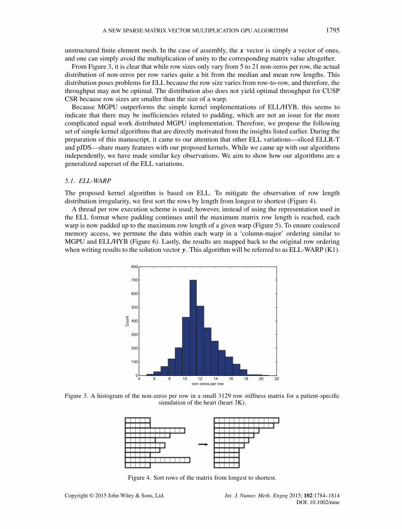
From Figure 3, it is clear that while row sizes only vary from 5 to 21 non-zeros per row, the actualdistribution of non-zeros per row varies quite a bit from the median and mean row lengths. Thisdistribution poses problems for ELL because the row size varies from row-to-row, and therefore, thethroughput may not be optimal. The distribution also does not yield optimal throughput for CUSPCSR because row sizes are smaller than the size of a warp.
Because MGPU outperforms the simple kernel implementations of ELL/HYB, this seems toindicate that there may be inefficiencies related to padding, which are not an issue for the morecomplicated equal work distributed MGPU implementation. Therefore, we propose the followingset of simple kernel algorithms that are directly motivated from the insights listed earlier. During thepreparation of this manuscript, it came to our attention that other ELL variations—sliced ELLR-Tand pJDS—share many features with our proposed kernels. While we came up with our algorithmsindependently, we have made similar key observations. We aim to show how our algorithms are ageneralized superset of the ELL variations.
5.1. ELL-WARP
The proposed kernel algorithm is based on ELL. To mitigate the observation of row lengthdistribution irregularity, we first sort the rows by length from longest to shortest (Figure 4).
A thread per row execution scheme is used; however, instead of using the representation used inthe ELL format where padding continues until the maximum matrix row length is reached, eachwarp is now padded up to the maximum row length of a given warp (Figure 5). To ensure coalescedmemory access, we permute the data within each warp in a ‘column-major’ ordering similar toMGPU and ELL/HYB (Figure 6). Lastly, the results are mapped back to the original row orderingwhen writing results to the solution vector y . This algorithm will be referred to as ELL-WARP (K1).
Figure 3. A histogram of the non-zeros per row in a small 3129 row stiffness matrix for a patient-specificsimulation of the heart (heart 3K).
Figure 4. Sort rows of the matrix from longest to shortest.
Copyright © 2015 John Wiley & Sons, Ltd. Int. J. Numer. Meth. Engng 2015; 102:1784–1814DOI: 10.1002/nme

1796 J. WONG, E. KUHL AND E. DARVE
Figure 5. Arrange rows into groups of warp size and then pad accordingly. In this figure, we use a warpsize = 4 only for purposes of illustration.
Figure 6. Reorder the first warp in Figure 5 in a coalesced column-major ordering.
The code is shown in Listing 2. K1 requires that a list of values and their column indices be paddedper warp, which are then sorted by row length and arranged in ‘column-major’ order. A list of theinitial offsets for each warp is given as well as a row mapping from the sorted row index to theoriginal row index.
The purpose of this arrangement is to exploit the relatively small variances in row lengths perwarp to reduce unnecessary padding in ELL and also to increase the amount of threads performingmeaningful operations. As values and column indices are zero padded, those values and column
Copyright © 2015 John Wiley & Sons, Ltd. Int. J. Numer. Meth. Engng 2015; 102:1784–1814DOI: 10.1002/nme

A NEW SPARSE MATRIX VECTOR MULTIPLICATION GPU ALGORITHM 1797
indices are cached and should not reduce the effectiveness of this algorithm if the variances withineach warp are in fact small. By having a fixed row length for each warp, one can reduce the amountof data needed to compute row sums in comparison with CSR and COO while reducing the numberof trivial instructions executed for padded entries in comparison with ELL. Thus, this kernel aimsto achieve an equally-distributed workload similar to MGPU in cases where there is some degree ofrow length regularity within each warp. Unfortunately, the final non-coalesced memory write to thesolution vector is a potential inefficiency for this kernel, which is otherwise coalesced in terms ofmemory access to values and column indices.
5.2. ELL-WARP with row reordering (K1r)
While reordering the rows of the matrix helps us achieve row length regularity within individ-ual warps, a straightforward SPMV operation with the row permuted matrix will yield a permutedsolution.
Ai;jxj D yi Ap.i/;jxj D yp.i/ (9)
Thus, the final memory store operation undoes this permutation, p.i/, such that the original orderingof the solution is preserved; however, this operation results in a non-coalesced memory storagepattern. To mitigate the necessity of performing a non-coalesced write within our kernel, the columnindices of the matrix and the vector x can be reordered such that the numbering of the correspondingentries in x and the solution vector are consistent. This is commonly performed in finite elementcomputations by renumbering the unknowns during the setup phase of most codes. Reordering thecolumns of the matrix and entries of x does not change the result of the solution vector.
Ai;jxj D yi Ai;f .j /xf .j / D yi (10)
By performing this reordering, we can essentially ignore the original row mapping necessary inK1 as the sorted solution vector is now numbered consistently with the newly arranged x0 vector.Unfortunately, the reordering of the column indices now produces a non-ordered access patternwhen reading values from the x0 vector. While the effects may be mitigated by using a texture cache,this is somewhat undesirable.
To further illustrate the reordering scheme, we considered a CSR ordered matrix for convenience.If xnum is the original ordering for x, then P is the new ordering such that the rows will be sortedaccordingly from longest to shortest.
xnum�1 2 3 4 5 6 7
�P�2 5 7 3 1 4 6
�The reordered vector, x0, and the reordered column indices, c0, are defined in the succeeding text,
where P is a permutation operator:
x0.�/ D x.P.�// (11)
c0.�/ D c.P�1.�// (12)
.�/ D P.P�1.�// (13)
Given the following single-row CSR matrix A, a dense vector of column indices c, and a densevector x
A D�7 8 9 10 2
�c D
�1 2 4 5 6
�x D
�1 2 3 4 5 6 7
�the K1r scheme described earlier will re-arrange the data such that the following results.
c0 D�5 1 6 2 7
�x0 D
�2 5 7 3 1 4 6
�This reordering scheme does not require that A be ordered but results in non-ordered columnindices, c0, which is possibly detrimental to maintaining ordered access from x0.
Copyright © 2015 John Wiley & Sons, Ltd. Int. J. Numer. Meth. Engng 2015; 102:1784–1814DOI: 10.1002/nme

1798 J. WONG, E. KUHL AND E. DARVE
5.3. K1r with sorted column index numbering (K1rs)
The following is a variation on K1r that attempts to fix the issue with non-ordered access to the x0
vector. The solution is to renumber the column indices of the matrix A. This requires a reorderingof the values of the matrix in each row such that the reordering of the column indices is sorted inorder after the reordering of the vector x.
Again using the previous single-row CSR matrix as an example, we sort c0 such that it is orderedfrom the smallest to largest indices within each row.
c00 D�1 2 5 6 7
�A00 D
�8 10 7 9 2
�The vector x0 remains the same; however, now, it is necessary to sort the values of A within eachrow to properly account for the changes in c0. The result is a intra-row reordered CSR matrix, A00,and an ordered set of corresponding column indices, c00.
5.4. ELL-WARP v2 (K2)
To accommodate the possibility of larger intra-warp row length variances, a multiple threads per rowvariation of K1 is proposed. For example, if there exist a small number of abnormally long rows, itmay be advantageous to process those rows with more threads while allowing the rest of the rowsin the matrix to be processed by K1.
A threshold value for the maximum number of entries a thread should be assigned is prescribed.If a row does not meet this criterion, the row is subdivided in half recursively until it meets thisrequirement. However, to avoid explicit thread synchronization within a block, if a row is longerthan 32� threshold, one warp will at the least process the entire row to maintain warp-to-warp rowindependence. The subdivision and repacking of the matrix is shown graphically in Figure 7.
The variation inevitably increases the amount of padding in comparison with K1 based on thethreshold value chosen. However, it allows unusually long rows to be processed more efficiently,
Figure 7. A threshold value (purple dashed line) is given, and the original padding in K1 is reorganized intosmaller more evenly distributed warps.
Copyright © 2015 John Wiley & Sons, Ltd. Int. J. Numer. Meth. Engng 2015; 102:1784–1814DOI: 10.1002/nme

A NEW SPARSE MATRIX VECTOR MULTIPLICATION GPU ALGORITHM 1799
Figure 8. Coloring represents the data for a particular thread. In this instance, four threads are used to processthe representative row. Data are arranged in column-major order, and then a parallel reduction step occurs
resulting with the final sum in the first entry of the output row.
while smaller rows retain the same padding as K1. The threshold parameter forces almost all warpsto process the same number of non-zero entries. The kernel now includes a simple parallel reductionloop, which reduces rows in a given warp efficiently using shared memory. This is seen in Figure 8for the first row of the representative warp in our illustrative example.
As rows are sorted initially, it is relatively easy to reprocess the original warp-sized row groupingsfrom K1 and subdivide the numbers of rows per warp as needed to meet the threshold criterion.Extra information per warp is necessary to dictate the row number per warp and also the number ofreductions needed per warp. However, this extra indexing information is minimal and results in twoextra integers retrieved from global memory per warp. The code for ELL-WARP v2 (K2) is shownin Listing 3.
5.5. K2 variations (K2r) and (K2rs)
Lastly, to avoid the final row mapping from sorted to non-sorted rows, the same variations proposedfor K1 can be simply applied directly to K2. The fundamental difference between K1 and K2 isin how the matrix is repackaged into blocks of data. In K2, the packaging is more regular withinblocks, whereas in K1, the packaging is more regular only within a given warp.
6. BENCHMARKS OF SPARSE-MATRIX VECTOR MULTIPLICATION METHODS
Our novel algorithms earlier are compared against several available standard SPMV algorithmsusing a set of sparse matrices commonly used in benchmarking SPMV methods [29, 42, 43].Because the K1 and K2 kernels were developed for finite element simulations of the heart, wehave also included three different refinements of a patient-specific heart mesh as part of the setof benchmark matrices. General information about each of the benchmark matrices is included inTable II.
Matrix structure properties vary substantially from matrix to matrix. It is apparent that cer-tain matrices, such as Circuit and Webbase, have a very skewed non-zero row length distribution.On the other hand, some matrices such as Epidemiology and QCD have very regular row lengthdistributions.
The following kernels were then chosen for comparison: CUSP-CSR and CUSP-HYB [32],CUSPARSE [33], MGPU [40], K1/r/rs, and K2/r/rs. The published MGPU results report the kerneltime by performing a large number of products Ax within a loop and reporting the average run-time per product. It was observed that the performance of the MGPU kernel varies depending on thenumber of iterations, with better performance at a higher number of iterations. However, in practice,
Copyright © 2015 John Wiley & Sons, Ltd. Int. J. Numer. Meth. Engng 2015; 102:1784–1814DOI: 10.1002/nme

1800 J. WONG, E. KUHL AND E. DARVE
a single product Ax is computed followed for some vector operations, after which further prod-ucts Ax are needed. Therefore, it is unclear to what extent the performance of the MGPU kernelreported for a large number of products Ax, computed immediately after one another, is relevant.Therefore, we will show results for one run of the kernels here, while the results for 1200 iterationscan be found in the Appendix A.1.
For each matrix used in the benchmark, kernel times are averaged over a specified number ofiteration runs. For the K1/r/rs kernels, different block sizes are varied from 32 to 256 threads byincrements of 32. Likewise, the same is performed for the K2/r/rs kernels except, in addition, dif-ferent maximum non-zero thresholds are varied from the minimum row length of the matrix to themaximum row length of the matrix. Lastly, for MGPU, the following number of values per thread isused: 4, 6, 8, 10, 12, and 16. After the parameters for K1, K2, and MGPU are acquired, the fastestaveraged times are found. The effective bandwidth is reported in Figure 9 and is defined as the rateof bytes processed from the matrix data by a kernel over time.
Copyright © 2015 John Wiley & Sons, Ltd. Int. J. Numer. Meth. Engng 2015; 102:1784–1814DOI: 10.1002/nme

A NEW SPARSE MATRIX VECTOR MULTIPLICATION GPU ALGORITHM 1801
Table II. Matrix benchmark information.
MatrixName nz nrows bytes minrow maxrow nz/nrows
Circuit 958,936 170,998 19,178,720 1 353 6Economics 1,273,389 206,500 25,467,780 1 44 7Epidemiology 2,100,225 525,825 42,004,500 2 4 4FEMAccelerator 2,624,331 121,192 52,486,620 8 81 22FEMCantilever 4,007,383 62,451 80,147,660 1 78 65FEMHarbor 2,374,001 46,835 47,480,020 4 145 51FEMShip 7,813,404 140,874 156,268,080 24 102 56FEMSpheres 6,010,480 83,334 120,209,600 1 81 73Heart 3K 37,035 3129 740,700 5 21 12Heart 5K 52,715 4563 1,054,300 6 22 12Heart 30K 367,443 28,639 7,348,860 6 24 13Protein 4,344,765 36,417 86,895,300 18 204 120QCD 1,916,928 49,152 38,338,560 39 39 39Webbase 3,105,536 1,000,005 62,110,720 1 4700 4WindTunnel 11,634,424 217,918 232,688,480 2 180 54
The number of non-zeros (nz), the number of rows (nrows), bytes, minimum row length (minrow),maximum row length (maxrow), and average number of non-zero values per row (nz/nrows) isreported for each benchmark matrix. The matrices highlighted (bold) are finite element meshes ofdifferent refinements of a patient-specific heart mesh.
Figure 9. Effective bandwidth benchmark results over matrices for one run are shown for CUSP-CSR (blue),CUSP-HYB (red), CUSPARSE (green), MGPU (purple), K1 (cyan), and K2 (orange).
All benchmarks were run on a single Asus ENGTX480 graphics card (CUDA Compute compati-bility 2.0) and on a PC with an Intel I7 950 CPU and 12 GB of memory. Kernels are compiled withoptimizations enabled (–O3), and kernels use the texture cache when possible. The results for a sin-gle iteration run is shown in Figure 9. The parameters for MGPU, K1, and K2 are shown for eachof the best performing kernels for each matrix in Table III.
The results for a single iteration indicate that our K1 and K2 algorithms perform well overall.For our patient-specific heart meshes, K1 and K2 algorithms perform better than the other testedalgorithms. MGPU performs best for two matrices: Economics and FEMCantilever. Meanwhile, K1and K2 algorithms perform well even for Economics and FEMCantilever and in general providethe best performance over the benchmarked matrices. Lastly, the effective bandwidth results varyslightly with the number of iterations for MGPU and CUSPARSE, where an increase in the number
Copyright © 2015 John Wiley & Sons, Ltd. Int. J. Numer. Meth. Engng 2015; 102:1784–1814DOI: 10.1002/nme

1802 J. WONG, E. KUHL AND E. DARVE
Table III. Benchmark best parameters for MGPU, K1 and K2.
MGPU K1 K2MatrixName valuesPerThread blocksize threshold Blocksize
Circuit 6 64 80 160Economics 6 64 7 96Epidemiology 6 128 4 128FEMAccelerator 6 64 58 64FEMCantilever 10 64 19 224FEMHarbor 10 96 128 96FEMShip 10 96 28 128FEMSpheres 10 96 47 128Heart 3K 12 32 7 256Heart 5K 10 64 10 192Heart 30K 10 64 21 64Protein 10 64 172 96QCD 10 224 39 96Webbase 6 32 658 128WindTunnel 10 96 38 96
of iterations improves performance. These results can be found in the Appendix. Despite thesevariances, the K1 and K2 kernels still outperform or are at least comparable with MGPU.
In many ways, it is quite surprising that a relatively simple kernel algorithm (22 lines) has com-parable performance to a sophisticated segmented scan algorithm in the case of MGPU (145 lines).Unlike other GPU SPMV algorithms, K1 and K2 are monolithic kernels, and extra kernel invoca-tions are unnecessary. However, the thread block size for K1 and K2 are generally different, andthus, their parameters must be found individually.
The effect of warp-level organization versus global data restructuring in HYB can be inferredfrom Figure 9 because K1 and K2 are partially warp-based variations of the ELL SPMV imple-mentation and thus related to the HYB format. The results from the two variations of ELL showdrastically different performance results for the majority of the benchmarked sparse matrices. K1and K2 reduce the amount of padding with respect to ELL and simultaneously reduce the amount ofmemory transactions needed for computing the SPMV operation in comparison with HYB, therebyproviding a dramatic increase in performance. K2 is used when there is a large difference in rowlength regularity and effectively handles outlier rows in a hybrid ELL-CSR-like manner. Together,K1 and K2 are substantially better than ELL and HYB for sparse matrices.
6.1. Cost of reordering matrix values
To determine whether it is beneficial overall to reorder the data in a ‘column-major’ coalesced pat-tern in SPMV applications for finite elements, we consider the following. If K1 and K2 are used tocalculate SPMV multiplications in the CG method, only one initial transpose of values is necessaryat the beginning of each Newton–Raphson iteration with the assumption that the assembler passes aCSR formatted matrix to the solver. Column indices do not need to be reordered, as we assume thatthe connectivity of the Lagrangian mesh does not change during the simulation; therefore, only thevalues of the tangent matrix change while the matrix structure remains constant. We can then deter-mine the number of CG iterations necessary, such that K1 and K2 will outperform CUSPARSE bythe following:
treorder C ˛twpk 6 ˛tcusparse (14)
where ˛ is the number of iterations necessary such that a reordering of data from CSR to ‘column-major’ provides a benefit for the CG solver. treorder is the time to reorder the CSR tangent matrix intoa coalesced K1-compatible and K2-compatible form. twpk and tcusparse are the SPMV operation timesfor K1/K2 and CUSPARSE, respectively. The following data are used to compare the differencesbetween reordering on the GPU and on the CPU. As our algorithm produces a reordering mapping
Copyright © 2015 John Wiley & Sons, Ltd. Int. J. Numer. Meth. Engng 2015; 102:1784–1814DOI: 10.1002/nme

A NEW SPARSE MATRIX VECTOR MULTIPLICATION GPU ALGORITHM 1803
for all non-zero entries during the initial scan, scatter operations are simply performed on the CPUusing a simple for loop, and the thrust::scatter() is used on the GPU [52].
From Table IV, it is fairly clear that CPU reordering is substantially slower than reorderingdirectly on the GPU even for small matrices (Heart, HeartCoarse, etc.). On average, GPU reorderingis five times faster than CPU reordering over all of the tested matrices. GPU reordering still takeslonger than the GPU SPMV kernel for the majority of matrices. However, even when reorderingon the CPU at every Newton–Raphson iteration for the finite element benchmark matrices, ˛CPU, iswithin the general number of iterations for most CG problems. On the other hand, GPU reorderingis very fast, and the benefits should be noticeable within 10 iterations for both K1 and K2 on aver-age. Thus, for the remaining number of iterations, the benefit of K1 and K2 over other kernels willbe evident.
Table IV. Comparison of ˛ ratios for the graphics processingunit and CPU for K1 and K2.
MatrixName ˛GPU,K1 ˛CPU,K1 ˛GPU,K2 ˛CPU,K2
Circuit 3 15 3 12Economics 3 12 3 13Epidemiology 2 20 2 21FEMAccelerator 3 12 3 12FEMCantilever 12 50 9 39FEMHarbor 7 27 7 28FEMShip 8 27 8 24FEMSpheres 10 34 10 34Heart 3K 1 4 1 4Heart 5K 1 5 1 5Heart 30K 3 10 3 10Protein 21 96 21 91QCD 4 17 4 17Webbase 1 1 2 12WindTunnel 8 26 8 24
˛ represents the number of sparse matrix vector operations nec-essary for the benefit of K1/K2 kernels to be apparent over tradi-tional non-reordered sparse matrix vector algorithms. The differentrefinements of our patient-specific meshes are in bold. ˛ D 1means that for that particular matrix, the cost of reordering a com-pressed sparse row matrix into a K1/K2-compatible form cannot beshown because twpk is slower than tcusparse.
Figure 10. Factor of reordering time to kernel time .treorder W twpk/ on the graphics processing unit (GPU) andCPU for K1 and K2 kernels are shown. Factors for K1 for the GPU are shown in blue, and for the CPU are
shown in green. For K2, GPU reordering is shown in red and in purple for the CPU.
Copyright © 2015 John Wiley & Sons, Ltd. Int. J. Numer. Meth. Engng 2015; 102:1784–1814DOI: 10.1002/nme

1804 J. WONG, E. KUHL AND E. DARVE
Table V. Description of the three different approaches to sorting and renumber-ing a kernel X, which is either kernel K1 or K2.
Kernel approach Description
KX Matrix element data are divided into sorted warp-sizedsegments and reordered with ‘column-major’ ordering.
KXr In addition to KX, x is reordered, and the column indicesof the matrix are renumbered accordingly to avoidnon-coalesced assignment.
KXrs In addition to KXr, the column indices are renumbered suchthat access to the x vector is ordered. The matrix values aresubsequently rearranged in a corresponding manner.
From Figure 10, one initially may discount the benefit of using any reordered kernels for globalfinite element tangent assembly. However, the ordering for finite element assembly can be arranged,such that the resulting ordering is already ‘column-major’ ordered. Likewise, the result of the assem-bly of the tangent matrix can also be arranged such that results are already coalesced and orderedproperly; thus, bypassing the need for reordering the matrix A altogether. Only, in this way, canthe performance of the synthetic benchmark results for K1 and K2 be obtained for finite elementassembly in real applications.
7. EFFECT OF INDIVIDUAL OPTIMIZATIONS
In this section, we evaluate different aspects of performance. We first investigate whether differentkernel level optimizations and the variations to K1 and K2 provide an improvement in performance.The cost-effectiveness of GPU data reordering is then compared and evaluated against CPU datareordering implementations.
A subset of the benchmark matrices were chosen to determine the effects of different kernel opti-mizations taken in the development of K1 and K2 and their variants. The matrices chosen wereCircuit, Epidemiology, FEMHarbor, Heart 3K, Heart 5K, Heart 30K, and QCD. The followingfactors were measured for an ELLWARP algorithm (KX): coalesced versus non-coalesced mem-ory access patterns, sorted versus unsorted rows, kernels that involve remapping versus those thatrenumber column indices and reorder the vector x (KX versus KXr), and, lastly, the differencesbetween two possible column numbering schemes (KXr versus KXrs). See Table V for a summaryof our notations for the different kernel variants.
First, we investigate the importance of coalesced memory access in Figure 11. In this test, wecompared our K1 kernel against a kernel where data were left in the standard CSR ‘row-major’ forminstead of a ‘column-major’ ordering that results in coalesced memory access within each warp. Asexpected, coalesced memory access patterns result in a dramatic reduction in computation time incomparison to non-coalesced memory access patterns. In fact, a coalesced memory access patternaccounts for a 1.5-fold to 9-fold increase in speed when using texture memory access and for a1.5-fold to 10-fold increase in speed without textures.
We also tested the effect of sorting matrix rows from longest to shortest (K1) and compared itto the equivalent algorithm where the ordering of rows of the original matrix and x vector are pre-served (non-sorted). As the non-sorted implementations must result in extra zero padding comparedwith the sorted ELLWARP implementations, the table in the succeeding text (Table VI) reports thedifference in padding and also shows the percentage of time difference with respect to a non-rowordered algorithm for K1. The time difference is defined as the K1 kernel time subtracted fromthe non-sorted K1 kernel time. The time-difference percentage is simply the percentage of timedifference with respect to the non-sorted kernel time.
The effect of sorting on performance is not entirely clear. For the majority of matrices, sortingthe matrices resulted in an increase in performance when using the texture memory cache; however,sorting may have detrimental effects on other matrices as shown for Epidemiology even when usingthe texture cache. On the other hand, without texture cache access, preserving the original row
Copyright © 2015 John Wiley & Sons, Ltd. Int. J. Numer. Meth. Engng 2015; 102:1784–1814DOI: 10.1002/nme

A NEW SPARSE MATRIX VECTOR MULTIPLICATION GPU ALGORITHM 1805
Figure 11. Comparison of coalesced ‘column-major’ data versus non-coalesced data ordering kernel timesfor K1.
Table VI. Benchmark data regarding the effects of sorting for K1 are shown in the succeeding text.
Circuit Epidemiology FEMHarbor Heart HeartCoarse HeartRefined QCD
Padding difference percentage (%) 59.89 0.14 33.67 29.60 33.73 30.03 0Time difference (textured; %) 21.16 �2.10 0.00 3.00 22.67 5.79 0.47Time difference (%) �17.38 �4.35 0.00 �28.22 10.42 �46.80 0.49
The padding difference percentage designates the percentage of padding that differs between the padded sorted andnon-sorted rows with the padded non-sorted representation as reference. A positive padding difference percentagemeans that the sorted K1 kernel reduces padding. The time difference percentage is defined as the time difference,the K1 kernel time subtracted from the non-sorted kernel time, divided by the non-sorted kernel time. A positivetime difference means that the K1 kernel is faster when sorted.
ordering results in significantly faster kernel times. Except for the Epidemiology matrix, the texturecache helps significantly, and the row-sorted texture cache kernel times are faster than the non-sorted kernel times without texture cache. However, from Table VI, it is evident that Epidemiologyand QCD have very similar row length regularity, and therefore, the effects of sorting may actuallydisrupt the ordered access pattern for x. Texture access is therefore not as helpful in those cases.Overall, sorting the rows greatly reduces the zero padding necessary, which is important in terms ofapplying SPMV operations in real situations.
Other tests were performed to compare the possible benefits from using the different kernelvariations K.�/r and K.�/rs, and their results can be found in the Appendix. From the results, theperformance improvement gained from reordering x to match the sorting of rows by length can bedirectly attributed to the avoiding of the non-coalesced assignment required in the original kernel.However, each of the variations only provides a small speedup in comparison with the precedingeffects of coalesced ordering for the matrix and longest-to-shortest reordering.
Overall, our results show that column-major coalesced memory access, use of textures, and sort-ing are very important. This corroborates key insights made in developing the ELL, HYB, andMGPU SPMV algorithms [29, 40] where column-major ordering can help achieve optimal memorythroughput while retaining a degree of flexibility with regard to the number of threads and matrixvalues per row. The effect of using the texture cache in accessing values from x is significant incases where access to the x is not already highly ordered, as in the case of Epidemiology. Lastly,while the effects of sorting rows from longest to shortest with the texture cache can be significant,the main benefit of the sorting is to reduce the amount of zero padding, which ultimately allows theK1 and K2 kernels to perform well even on larger highly unstructured meshes.
While the different variations provided additional benefits over the original K1 and K2 algorithms,the effects are less significant in comparison with the effects of column-major ordering and the useof the texture cache. Unfortunately, embedding alternate renumbering schemes adds some additionalcomplexity to the finite element implementation. Therefore, if every bit of performance must beobtained, one would ideally use a pre-reordered x variation (Kr, Krs). While the speedup gains arecompounded between K versus Kr and Kr versus Krs, proper modifications should yield substantial
Copyright © 2015 John Wiley & Sons, Ltd. Int. J. Numer. Meth. Engng 2015; 102:1784–1814DOI: 10.1002/nme

1806 J. WONG, E. KUHL AND E. DARVE
improvements in SPMV computation speed. However, as general drop-in SPMV replacements, K1and K2 seem to perform quite well for many applications.
8. FINITE ELEMENT COMPARISON BETWEEN GRAPHICS PROCESSING UNIT ANDMULTI-CORE
In the final set of results, we compare the performance of our finite element GPU framework againsta multi-core PETSc implementation of the same code. For the GPU SPMV implementation, we usethe best parameters found for K1 and K2 from Tables VIII and IX for 50 iterations. For MGPU(Table VII), we simply have chosen valuesPerThread = 6 and 10 for reference. We look atfour different successive refinements of the Heart mesh: 3k, 5k, 30k, and 50k nodes. The benchmarkresults for the 50k mesh use the same parameters for K1 and K2 SPMV kernels as those foundfor Heart 30K. For simplicity, the GPU finite element assembly implementation uses CUSPARSEfor SPMV to assemble the global tangent matrix and global residual vector. For the multi-corePETSc implementation, we used a Jacobi preconditioned CG solver when possible; however, therewere convergence issues with the simple Jacobi preconditioner for the 50k mesh. However, for thepurposes of comparison, we also show the results of our PETSc implementation using the block-Jacobi preconditioner for all four mesh refinements. In these results, we use a CPU-based reorderingfor MGPU, K1, and K2. On the CPU, the following results are reported for the PETSc Jacobi andblock preconditioners running on 1, 2, 3, and 4 cores. CPU reordering of the matrix was used forthese results.
The resulting speedup for the different tests with a single process PETSc block-Jacobi solver withstandard finite element assembly as reference is shown in Figure 12. Several general observationscan be made. First, the multi-core CPU PETSc implementation does not scale linearly. The block-Jacobi preconditioner CG solver is slightly faster than the Jacobi preconditioner counterpart, butthe parallel speedups on multiple cores are roughly the same. The GPU CG solver with CPU finiteelement assembly implementation is marginally slower than the three-core PETSc implementation.The GPU finite element implementations are at least twice as fast compared with the quad processPETSc implementations.
Overall, the GPU CG solver implementations with finite element assembly start with a twofoldspeedup for the 3129-node mesh and increase to a factor of 2.5 for the 50,000 node heart mesh.CUSP-CSR and CUSPARSE-CSR seem to perform better in comparison with K1 and K2 as thenumber of nodes increases. It should be noted that with GPU reordering, the performance of K1and K2 kernels improves slightly; however, the CUSP-CSR and CUSPARSE-based CG solvers stillinitially perform better that the K1 and K2 kernels. This point will be clarified later in this section.
Table VII. Benchmark best MGPU valuesPerThread parameter.
MatrixName mgpu [1] best mgpu [50] best mgpu [1200] best
Circuit 6 6 4Economics 6 6 6Epidemiology 6 4 4FEMAccelerator 6 6 4FEMCantilever 10 10 10FEMHarbor 10 12 16FEMShip 10 10 10FEMSpheres 10 12 12Heart 3K 12 10 10Heart 5K 10 8 8Heart 30K 10 10 6Protein 10 16 16QCD 10 10 10Webbase 6 4 4WindTunnel 10 10 10
The number of repeated sparse matrix vector iterations is denoted in brackets.
Copyright © 2015 John Wiley & Sons, Ltd. Int. J. Numer. Meth. Engng 2015; 102:1784–1814DOI: 10.1002/nme

A NEW SPARSE MATRIX VECTOR MULTIPLICATION GPU ALGORITHM 1807
Figure 12. The resulting factor of the increase in speed is shown for the graphics processing unit (GPU)conjugate gradient (CG) solver and GPU finite element method. The factor of the increase in speed is definedas the ratio of the computation time of the single core PETSc block-Jacobi CG solver compared with thecomputation time of the highlighted GPU sparse matrix vector (SPMV) algorithms denoted by the differentcolors. Results using a GPU CG solver with a standard single core CPU-based element assembly routine areshown (top). Results for GPU CG solver and GPU element assembly implementations are shown (bottom)
together with multi-core CPU PETSc implementation speedup results.
MGPU also performs well but is the poorest performing kernel in all cases. On the other hand, thefully-GPU finite element implementation for K1 and K2 ranges from a speedup factor of 5 to 12as the mesh is subsequently refined. Again, CUSPARSE-CSR and CUSP perform better relative toMGPU as the mesh size increases; however, K1 and K2 kernels are only initially slower than CUSP-CSR. At larger mesh sizes of 30k and 50k nodes, K1 and K2 outperform CUSP-CSR even whenusing CPU data reordering.
The performance results found in the two finite element implementations do not seem to matchthose predicted by the synthetic benchmark. Namely, CUSP and CUSPARSE kernels scale signifi-cantly better than expected and in general outperform MGPU. It was found that K1 and K2 kernelsactually outperform the best CUSP and CUSPARSE kernels results after adjusting the parametersto the K1 and K2 kernels empirically from the acquired best results for 50 iterations (Tables VIIIand IX) even without GPU reordering. This finding indicates that more work must be carried out in
Copyright © 2015 John Wiley & Sons, Ltd. Int. J. Numer. Meth. Engng 2015; 102:1784–1814DOI: 10.1002/nme

1808 J. WONG, E. KUHL AND E. DARVE
Table VIII. Benchmark best K1 blocksize parameter.
MatrixName K1 [1] best K1 [50] best K1 [1200] best
Circuit 64 64 64Economics 64 64 64Epidemiology 128 128 128FEMAccelerator 64 64 64FEMCantilever 64 64 64FEMHarbor 96 96 96FEMShip 96 96 96FEMSpheres 96 96 96Heart 3K 32 32 32Heart 5K 64 32 64Heart 30K 64 64 64Protein 64 96 96QCD 224 224 224Webbase 32 32 32WindTunnel 96 96 96
The number of repeated sparse matrix vector iterations is denoted inbrackets.
Table IX. Benchmark K2 best threshold and blocksize parameters.
K2 [1] K2 [50] K2 [1200]MatrixName threshold blocksize threshold blocksize threshold blocksize
Circuit 80 160 38 128 112 160Economics 7 96 7 96 7 96Epidemiology 4 128 4 128 4 128FEMAccelerator 58 64 57 64 58 64FEMCantilever 19 224 19 224 19 224FEMHarbor 128 96 132 96 139 96FEMShip 28 128 27 128 27 128FEMSpheres 47 128 81 96 81 96Heart 3K 7 256 7 256 6 192Heart 5K 10 192 13 96 6 192Heart 30K 21 64 17 64 17 64Protein 172 96 167 96 171 96QCD 39 96 39 224 39 128Webbase 658 128 682 128 672 128WindTunnel 38 96 37 96 38 96
The number of repeated sparse matrix vector iterations is denoted in brackets.
developing a better representative benchmark to determine the best parameters for K1 and K2 forfinite element applications because the resulting best parameters for our finite element applicationsapparently do not match closely those found in our synthetic benchmarks.
9. CONCLUSION
While the results have been very promising for our kernels, we believe these algorithms can befurther improved both in terms of analysis and implementation of the algorithms in real applications.Reordering of values is still expensive compared with the actual SPMV computation time. Luckily,it is possible to hide the reordering bottleneck within the assembly routine. This can be performedby first reordering the location where each element stores its elemental stiffness and residual entriessuch that the kernel can directly use the stored matrix to generate a resulting global stiffness andresidual matrix that is already reordered for the CG solver.
Because this particular physical problem is assembly heavy, improvements and optimizations tothe finite element assembly operation will result in very substantial speed improvements in addition
Copyright © 2015 John Wiley & Sons, Ltd. Int. J. Numer. Meth. Engng 2015; 102:1784–1814DOI: 10.1002/nme

A NEW SPARSE MATRIX VECTOR MULTIPLICATION GPU ALGORITHM 1809
to improvements to SPMV operations. The shared-memory non-zero assembly operation [21] canbe used to reduce global memory use and increase computational density. Coloring techniques mayalso be an alternative strategy in gaining additional performance in assembling the matrices fromelement matrices to global matrices. Another alternative is to leverage streaming algorithms to per-form assembly operations and compute element quantities simultaneously to reduce global memoryusage and potential race conditions.
Lastly, the slight differences between the optimal parameters for GPU CG solvers and the optimalparameters for GPU finite element implementations highlight potential avenues of improvement forour novel algorithms. Because the structure and access pattern of each mesh and matrix can beanalyzed beforehand, it would be extremely beneficial to develop a metric for determining goodpartitioning parameters for the K1 and K2 algorithms a priori. Given the relatively simplicity ofthis algorithm, such a study should be possible and would further increase the utility of these ELL-WARP algorithms.
In conclusion, we have shown how key insights from the ELL, HYB, pJDS, and ModernGPUSPMV algorithms have led to the development of new, efficient SPMV algorithms that perform wellover a large range of sparse matrices. The effects of different optimizations have been examined andultimately lead to faster SPMV computation times. Lastly, this study highlights the potential use ofGPUs for general finite element simulations.
ACKNOWLEDGEMENTS
Part of this research was done at Stanford University, and was supported in part by the U.S. Army ResearchLaboratory, through the Army High Performance Computing Research Center, Cooperative AgreementW911NF-07-0027. This material is also based upon work supported by the Department of Energy NationalNuclear Security Administration, under Award Number DE-NA0002373-1. This work was also partlysupported by the National Institutes of Health, grant U01 HL119578.
APPENDIX
The following sections have been included in the appendix to highlight interesting observationsand results that support and add value to this paper yet are not key findings to this work. Theappendix is organized into three subsections: a first section, regarding the optimal parameters foundfor the MGPU, K1, and K2 kernels using our particular hardware; a second section, comparing thedifferences between the kernel variations, and a final section, where GPU reordering is utilized toimprove the performance of K1 and K2 kernels in the context of SPMV operations.
Figure A.1. Effective bandwidth benchmark results of matrices for 1200 iterations.
Copyright © 2015 John Wiley & Sons, Ltd. Int. J. Numer. Meth. Engng 2015; 102:1784–1814DOI: 10.1002/nme
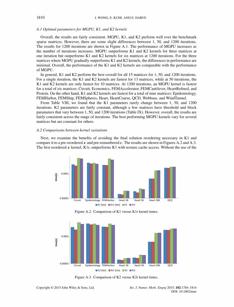
1810 J. WONG, E. KUHL AND E. DARVE
A.1 Optimal parameters for MGPU, K1, and K2 kernels
Overall, the results are fairly consistent. MGPU, K1, and K2 perform well over the benchmarksparse matrices. However, there are some slight differences between 1, 50, and 1200 iterations.The results for 1200 iterations are shown in Figure A.1. The performance of MGPU increases asthe number of iterations increases. MGPU outperforms K1 and K2 kernels for three matrices atone iteration but outperforms K1 and K2 kernels for six matrices at 1200 iterations. For the threematrices where MGPU gradually outperforms K1 and K2 kernels, the differences in performance areminimal. Overall, the performance of the K1 and K2 kernels are comparable with the performanceof MGPU.
In general, K1 and K2 perform the best overall for all 15 matrices for 1, 50, and 1200 iterations.For a single iteration, the K1 and K2 kernels are fastest for 13 matrices, while at 50 iterations, theK1 and K2 kernels are only fastest for 10 matrices. At 1200 iterations, an MGPU kernel is fastestfor a total of six matrices: Circuit, Economics, FEMAccelerator, FEMCantilever, HeartRefined, andProtein. On the other hand, K1 and K2 kernels are fastest for a total of nine matrices: Epidemiology,FEMHarbor, FEMShip, FEMSpheres, Heart, HeartCoarse, QCD, Webbase, and WindTunnel.
From Table VIII, we found that the K1 parameters rarely change between 1, 50, and 1200iterations. K2 parameters are fairly constant, although a few matrices have threshold and blockparameters that vary between 1, 50, and 1200 iterations (Table IX). However, overall, the results arefairly consistent across the range of iterations. The best performing MGPU kernels vary for severalmatrices but are constant for others.
A.2 Comparisons between kernel variations
Next, we examine the benefits of avoiding the final solution reordering necessary in K1 andcompare it to a pre-reordered x and pre-renumbered c. The results are shown in Figures A.2 and A.3.The first reordered x kernel, K1r, outperforms K1 with texture cache access. Without the use of the
Figure A.2. Comparison of K1 versus K1r kernel times.
Figure A.3. Comparison of K2 versus K2r kernel times.
Copyright © 2015 John Wiley & Sons, Ltd. Int. J. Numer. Meth. Engng 2015; 102:1784–1814DOI: 10.1002/nme

A NEW SPARSE MATRIX VECTOR MULTIPLICATION GPU ALGORITHM 1811
Figure A.4. Comparison of kernel times to investigate the cost of the final remapping to the originalreordering versus K1r.
Figure A.5. Comparison of K1r versus K1rs kernel times.
Figure A.6. Comparison of K2r versus K2rs kernel times.
texture cache, K1r outperforms K1, except in the case of the HeartRefined mesh. Likewise, with thetexture cache enabled, K2r outperforms K2 but is sometimes slower without texture cache access.The effect of reordering x is generally beneficial but is similar to the effect of sorting by row lengthwhere texture cache access for the well-ordered matrices such as Epidemiology and QCD result inonly slight differences between texture and non-texture cache results.
To determine the cost of the final solution remapping, the K1r kernel was modified to perform thefinal solution remapping that results in a solution y that matches the original numbering for x andthe results are reported in Figure A.4. In all cases, the cost of remapping is more than K1r. For K1rwith the use of the texture cache, the final solution remapping costs between 1% and 11.5% of thecomputation time of K1r. Whereas without the texture cache, remapping costs between 0.8% and8% of the computation time of K1r. Similar results were found for K2r.
Next, we examine the improvement of K1rs over K1r and K2rs over K2r in Figures A.5 and A.6.Other than the QCD and Epidemiology matrix cases, which are already very well ordered, the values
Copyright © 2015 John Wiley & Sons, Ltd. Int. J. Numer. Meth. Engng 2015; 102:1784–1814DOI: 10.1002/nme

1812 J. WONG, E. KUHL AND E. DARVE
and row-sorted versions of both kernels are marginally faster. K1rs is faster than K1r by 1.75% to7.25% with the texture cache and by 4% to 23.5% without the texture cache for matrices other thanQCD and Epidemiology. K2rs is faster than K1r by 1% to 7.5% with the texture cache and 0.25% to21% without the texture cache for matrices other than QCD and Epidemiology. K1rs and K2rs areslower than their Kr counterparts for the Epidemiology case by less than 0.25% with and without thetexture cache. For the QCD case, the row-sorted reordered kernels are slower by 0.25% and 3.25%.
REFERENCES
1. Elsen E, LeGresley P, Darve E. Large calculation of the flow over a hypersonic vehicle using a GPU. Journal ofComputational Physics 2008; 227(24):10148–10161.
2. Haase G, Liebmann M, Douglas C, Plank G. A parallel algebraic multigrid solver on graphics processing units. InHigh Performance Computing and Applications, vol. 5938, Zhang W, Chen Z, Douglas C, Tong W (eds)., LectureNotes in Computer Science. Springer: Berlin / Heidelberg, 2010; 38–47.
3. Taylor Z, Comas O, Cheng M, Passenger J, Hawkes D, Atkinson D, Ourselin S. On modelling of anisotropicviscoelasticity for soft tissue simulation: numerical solution and GPU execution. Medical Image Analysis 2009;13(2):234–244.
4. Pratx G, Xing L. GPU computing in medical physics: a review. Medical Physics 2011; 38(5):2685–2697.5. Joldes GR, Wittek A, Miller K. Real-time nonlinear finite element computations on GPU—application to neurosur-
gical simulation. Computer methods in applied mechanics and engineering 2010; 199(49):3305–3314.6. Taylor ZA, Cheng M, Ourselin S. High-speed nonlinear finite element analysis for surgical simulation using graphics
processing units. IEEE Transactions on Medical Imaging 2008; 27(5):650–663.7. Buatois L, Caumon G, Levy B. Concurrent number cruncher: a GPU implementation of a general sparse linear solver.
International Journal of Parallel, Emergent and Distributed Systems 2009; 24(3):205–223.8. Bolz J, Farmer I, Grinspun E, Schroder P. Sparse matrix solvers on the GPU: conjugate gradients and multigrid. ACM
Transactions on Graphics 2003; 22(3):917–924.9. Goddeke D, Buijssen S, Wobker H, Turek S. GPU acceleration of an unmodified parallel finite element Navier–Stokes
solver. International Conference on High Performance Computing Simulation, 2009. HPCS ’09, Leipzig, Germany,June 21–24 2009; 12–21.
10. Göddeke D, Strzodka R, Turek S. Accelerating double precision FEM simulations with GPUs. Proceedings of ASIM2005, 2005; 139-144.
11. Göddeke D, Strzodka R, Mohd-Yusof J, McCormick P, Wobker H, Becker C, Turek S. Using GPUs to improvemultigrid solver performance on a cluster. International Journal of Computational Science and Engineering 2008;4(1):36–55.
12. Bolz J, Farmer I, Grinspun E, Schröder P. Sparse matrix solvers on the GPU: conjugate gradients and multigrid. ACMTransactions on Graphics 2003; 22:917–924.
13. Rodriguez-Navarro J, Susin A. Nonstructured meshes for cloth GPU simulation using FEM. VRIPHYS, Madrid,Spain, 2006; 1–7.
14. Göddeke D. Fast and Accurate Finite-Element Multigrid Solvers for PDE Simulations on GPU Clusters. LogosVerlag Berlin GmbH: Berlin, Germany, 2011.
15. Turek S, Göddeke D, Becker C, Buijssen SHM, Wobker H. FEAST—realisation of hardware-oriented numerics forHPC simulations with finite elements. Concurrency and Computation: Practice and Experience 2010; 6:2247–2265.Special Issue Proceedings of ISC 2008.
16. Klöckner A, Warburton T, Bridge J, Hesthaven JS. Nodal discontinuous Galerkin methods on graphics processors.Journal of Computational Physics 2009; 228(21):7863–7882.
17. Komatitsch D, Micha D, Erlebacher G. Porting a high-order finite-element earthquake modeling application toNVIDIA graphics cards using CUDA. Journal of Parallel and Distributed Computing 2009; 69(5):451–460.
18. Komatitsch D, Erlebacher G, Göddeke D, Michéa D. High-order finite-element seismic wave propagation modelingwith mpi on a large GPU cluster. Journal of Computational Physics 2010; 229(20):7692–7714.
19. Tejada E, Ertl T. Large steps in GPU-based deformable bodies simulation. Simulation Modelling Practice and Theory2005; 13(8):703–715.
20. Markall G, Slemmer A, Ham D, Kelly P, Cantwell C, Sherwin S. Finite element assembly strategies on multi-coreand many-core architectures. International Journal for Numerical Methods in Fluids 2013; 71(1):80–97.
21. Cecka C, Lew AJ, Darve E. Assembly of finite element methods on graphics processors. International Journal forNumerical Methods in Engineering 2011; 85(5):640–669.
22. Cecka C, Lew A, Darve E. Application of assembly of finite element methods on graphics processors for real-timeelastodynamics. GPU Computing Gems Jade Edition 2010:187–205.
23. Dziekonski A, Sypek P, Lamecki A, Mrozowski M. Finite element matrix generation on a GPU. Progress InElectromagnetics Research 2012; 128:249–265.
24. Dziekonski A, Sypek P, Lamecki A, Mrozowski M. Accuracy, memory, and speed strategies in GPU-based finite-element matrix-generation. IEEE Antennas and Wireless Propagation Letters 2012; 11:1346–1349.
25. Markall GR, Ham DA, Kelly PH. Towards generating optimised finite element solvers for GPUs from high-levelspecifications. Procedia Computer Science 2010; 1(1):1815–1823.
Copyright © 2015 John Wiley & Sons, Ltd. Int. J. Numer. Meth. Engng 2015; 102:1784–1814DOI: 10.1002/nme

A NEW SPARSE MATRIX VECTOR MULTIPLICATION GPU ALGORITHM 1813
26. Lionetti FV, McCulloch AD, Baden SB. Source-to-source optimization of CUDA C for GPU accelerated cardiac cellmodeling. In Proceedings of the 16th international Euro-Par conference on Parallel processing: Part I, EuroPar’10.Springer-Verlag: Berlin, Heidelberg, 2010; 38–49.
27. Vigmond EJ, Boyle PM, Leon L, Plank G. Near-real-time simulations of biolelectric activity in small mammalianhearts using graphical processing units. Conference Proceedings of the IEEE Engineering in Medicine and BiologySociety 2009; 2009:3290–3293.
28. Bartocci E, Cherry EM, Glimm J, Grosu R, Smolka SA, Fenton FH. Toward real-time simulation of cardiac dynamics.In Proceedings of the 9th International Conference on Computational Methods in Systems Biology, CMSB ’11. ACM:New York, NY, USA, 2011; 103–112.
29. Bell N, Garland M. Implementing sparse matrix-vector multiplication on throughput-oriented processors. In Pro-ceedings of the Conference on High Performance Computing Networking, Storage and Analysis, SC ’09. ACM: NewYork, NY, USA, 2009; 18:1–18:11.
30. Nvidia C. CUDA C programming guide, PG-02829-001_v5.0 design guide, 2012.31. Bell N, Garland M. Efficient sparse matrix-vector multiplication on CUDA. Technical Report NVIDIA Technical
Report NVR-2008-004, NVIDIA Corporation, 2008.32. Bell N, Garland M. CUSP: a C++ templated sparse matrix library, 2013. (Available from: http://cusplibrary.github.
io), version 0.3.0. (Accessed on 2012).33. Nvidia C. Cusparse library: NVIDIA Corporation: Santa Clara, California, 2011. (Available from: https://developer.
nvidia.com/cusparse).34. Vazquez F, Garzon E, Martinez J, Fernandez J. The sparse matrix vector product on GPUs. Proceedings of the
2009 International Conference on Computational and Mathematical Methods in Science and Engineering 2009; 2:1081–1092.
35. Vazquez F, Ortega G, Fernandez JJ, Garzon EM. Improving the performance of the sparse matrix vector product withGPUs. In Proceedings of the 2010 10th IEEE International Conference on Computer and Information Technology,CIT ’10. IEEE Computer Society: Washington, DC, USA, 2010; 1146–1151.
36. Monakov A, Lokhmotov A, Avetisyan A. Automatically tuning sparse matrix-vector multiplication for GPU archi-tectures. In Proceedings of the 5th international conference on High Performance Embedded Architectures andCompilers, HiPEAC’10. Springer-Verlag: Berlin, Heidelberg, 2010; 111–125.
37. Dziekonski A, Lamecki A, Mrozowski M. A memory efficient and fast sparse matrix vector product on a GPU.Progress In Electromagnetics Research 2011; 116:49–63.
38. Vuduc RW, Moon HJ. Fast sparse matrix-vector multiplication by exploiting variable block structure. In Proceedingsof the First international conference on High Performance Computing and Communications, HPCC’05. Springer-Verlag: Berlin, Heidelberg, 2005; 807–816.
39. Monakov A, Avetisyan A. Implementing blocked sparse matrix-vector multiplication on NVIDIA GPUs. In Embed-ded Computer Systems: Architectures, Modeling, and Simulation, vol. 5657, Bertels K, Dimopoulos N, Silvano C,Wong S (eds)., Lecture Notes in Computer Science. Springer: Berlin / Heidelberg, 2009; 289–297.
40. Baxter S. Modern GPU libraries, 2011. (Available from: http://github.com/seanbaxter/mgpu/).41. Kreutzer M, Hager G, Wellein G, Fehske H, Basermann A, Bishop AR. Sparse matrix-vector multiplication on
GPGPU clusters: a new storage format and a scalable implementation. In Proceedings of the 2012 IEEE 26th Inter-national Parallel and Distributed Processing Symposium Workshops & PhD Forum, IPDPSW ’12. IEEE ComputerSociety: Washington, DC, USA, 2012; 1696–1702.
42. Williams S, Oliker L, Vuduc R, Shalf J, Yelick K, Demmel J. Optimization of sparse matrix-vector multiplication onemerging multicore platforms. Parallel Computing 2009; 35(3):178–194.
43. Davis T, Hu Y. et al.. Sparse matrix collection. (Available from: http://www.cise.ufl.edu/research/sparse/mat/Williams/README.txt), http://www.cise.ufl.edu/research/sparse/matrices/Williams/index.html, http://www.cise.ufl.edu/research/sparse/matrices/index.html.
44. Kreutzer M, Hager G, Wellein G, Fehske H, Bishop AR. A unified sparse matrix data format for modern processorswith wide SIMD units. Technical Report 1307.6209, 2013. arXiv.
45. Aliev RR, Panfilov AV. A simple two-variable model of cardiac excitation. Chaos, Solitons & Fractals 1996;7(3):293–301.
46. Göktepe S, Kuhl E. Computational modeling of cardiac electrophysiology: a novel finite element approach.International Journal for Numerical Methods in Engineering 2009; 79(2):156–178.
47. Wong J, Göktepe S, Kuhl E. Computational modeling of electrochemical coupling: a novel finite element approachtowards ionic models for cardiac electrophysiology. Computer Methods in Applied Mechanics and Engineering 2011;200(45–46):3139–3158.
48. Simo J. A framework for finite strain elastoplasticity based on maximum plastic dissipation and the multiplicativedecomposition. Part II: computational aspects. Computer Methods in Applied Mechanics and Engineering 1988;68(1):1–31.
Copyright © 2015 John Wiley & Sons, Ltd. Int. J. Numer. Meth. Engng 2015; 102:1784–1814DOI: 10.1002/nme

1814 J. WONG, E. KUHL AND E. DARVE
49. Balay S, Brown J, Buschelman K, Eijkhout V, Gropp WD, Kaushik D, Knepley MG, McInnes LC, Smith BF, ZhangH. PETSc users manual. Technical Report ANL-95/11 - Revision 3.3, Argonne National Laboratory, 2012.
50. Huthwaite P. Accelerated finite element elastodynamic simulations using the GPU. Journal of Computational Physics2014; 257:687–707.
51. Plaszewski P, Banas K, Maciol P. Higher order FEM numerical integration on GPUs with OpenCL. IMCSIT, Wisła,Poland, 2010; 337–342.
52. Hoberock J, Bell N. Thrust: a parallel template library, 2010. (Available from: http://www.meganewtons.com/),version 1.3.0.
Copyright © 2015 John Wiley & Sons, Ltd. Int. J. Numer. Meth. Engng 2015; 102:1784–1814DOI: 10.1002/nme