A New Solution to the Random Assignment Problem · PDF fileJournal of Economic Theory 100, 295 328 (2001) A New Solution to the Random Assignment Problem Anna Bogomolnaia Department

Journal of Economic Theory 100, 295�328 (2001)

A New Solution to the Random Assignment Problem

Anna Bogomolnaia

Department of Economics, Southern Methodist University, P.O. Box 750496,Dallas, Texas 75275-0496

annab�mail.smu.edu

and

Herve� Moulin

Department of Economics, Rice University, MS 22, P.O. Box 1892,Houston, Texas 77251-1892

moulin�rice.edu

Received August 30, 1999; final version received June 2, 2000;published online March 29, 2001

A random assignment is ordinally efficient if it is not stochastically dominatedwith respect to individual preferences over sure objects. Ordinal efficiency implies(is implied by) ex post (ex ante) efficiency. A simple algorithm characterizes ordinallyefficient assignments: our solution, probabilistic serial (PS), is a central element withintheir set. Random priority (RP) orders agents from the uniform distribution, then letsthem choose successively their best remaining object. RP is ex post, but not alwaysordinally, efficient. PS is envy-free, RP is not; RP is strategy-proof, PS is not. Ordinalefficiency, Strategyproofness, and equal treatment of equals are incompatible. Journalof Economic Literature Classification Numbers: C78, D61, D63. � 2001 Academic Press

Key Words: random assignment; ordinal; ex post or ex ante efficiency; strategyproof-ness; envy-free.

1. TWO PREVIOUS SOLUTIONS TO THE RANDOMASSIGNMENT PROBLEM

The assignment problem is the allocation problem where n objects areto be allocated among n agents, and each agent is to receive exactly oneobject. Examples include the assignment of jobs to workers, of rooms tohousemates, of time slots to users of a common machine, and so on (seeRoth and Sotomayor [14], Abdulkadiroglu and So� nmez [1]).

Using a lottery is one of the oldest tricks (going further back than theBible; see Hofstee [9]) to restore fairness in such problems.1 Suppose we

doi:10.1006�jeth.2000.2710, available online at http:��www.idealibrary.com on

2950022-0531�01 �35.00

Copyright � 2001 by Academic PressAll rights of reproduction in any form reserved.

1 Another standard trick is to use monetary compensations; see Leonard [12], Demange[5]. Here we assume that money is not available.

must allocate a single (desirable) object among several agents: tossing a fairdie is obviously the uniquely optimal method.2 The simplest extension ofthis method to the case of n heterogeneous objects and n agents is the familiarmechanism that we call random priority3 : draw at random an ordering ofthe agents from the uniform distribution and then let them successivelychoose an object in that order (so the first agent in the ordering gets firstpick and so on). This method has been around for a long time, althoughonly two papers in the economic literature discuss it: Zhou [19] andAbdulkadiroglu and So� nmez [1].

From the point of view of mechanism design, random priority is fair (atleast in the sense of equal treatment of equals) and incentive compatible (inthe sense of strategyproofness), but it is not efficient when the agents areendowed with Von Neumann�Morgenstern preferences over random alloca-tions (lotteries over objects), see Zhou [19].4

A second, more subtle, solution to the random assignment problem wasproposed by Hylland and Zeckhauser [10]. It adapts the competitive equi-librium with equal incomes solution for the fair division of unproducedcommodities (Varian [18], Thomson and Varian [17]) to the randomassignment model: a VNM utility function over random allocations of(indivisible) objects is viewed as a linear utility over vectors of ``shares'' ofthese objects, where the share of an object is the probability of receiving itin the eventual assignment. This solution, denoted CEEI, is fair in the senseof no envy (a criterion that the RP assignment does not always meet; seeProposition 1 in Section 7). It is also efficient with respect to the profile ofVNM utility functions, yet it is not strategyproof. In fact, Zhou [19](proving a conjecture formulated in Gale [7]) shows that there does notexist any strategyproof mechanism eliciting individual VNM utility func-tions and achieving both efficiency (Pareto optimality w.r.t. these utilityfunctions) and equity (in the very weak sense of equal treatment of equals).

The RP assignment is appealing on two accounts. First it is ex postefficient, that is to say every deterministic assignment that is selected withpositive probability is Pareto optimal. This is a weaker property than exante efficiency, namely efficiency with respect to the profile of VNM utilityfunctions, as discussed above. Second, the RP assignment can be computed

296 BOGOMOLNAIA AND MOULIN

2 For a formal statement see comment b in Section 9.3 Also called random serial dictatorship by Abdulkadiroglu and So� nmez [1].4 An example follows, with three agents, three objects and the VNM utilities: u1(a)=1,

u1(b)=0.8, u1(c)=0, for i=2, 3: ui (a)=1, ui (b)=0.2, ui (c)=0. The random priority assign-ment gives a 1�3 chance of every object to each agent (because their preferences over sureobjects coincide) and a profile of expected utilities (0.6, 0.4, 0.4). But assigning object b toagent 1 for sure and objects a, c randomly between agents 2, 3 yields the expected utilities(0.8, 0.5, 0.5).

or implemented from the profile of preferences over sure objects. Forany given ordering of the agents, we compute the best available object foreach agent in turn, and this does not require knowledge of the prefer-ences over lotteries (random objects). Contrast this simplicity with thecomputation of the CEEI solution, which requires us to elicit the profile offull-fledged VNM utility functions and to solve a difficult fixed-pointproblem (of which the solution may not be unique). We submit that thesimplicity of information gathering and implementation of the RP assign-ment makes the corresponding mechanism more appealing than the CEEIone.

We call a mechanism that elicits only individual preferences over sureobjects ordinal (whereas a cardinal mechanism collects a full-fledged VNMutility function from every agent). The restriction to ordinal mechanisms isthe central assumption in this paper.5 It can be justified by the limitedrationality of the agents participating in the mechanism. There is convincingexperimental evidence that the representation of preferences over uncertainoutcomes by VNM utility functions is inadequate (see, e.g., Kagel and Roth[11]). One interpretation of this literature is that the formulation of rationalpreferences over a given set of lotteries is a complex process that most agentsdo not engage into if they can avoid it. An ordinal mechanism allows theparticipants to formulate only this part of their preferences that does notrequire to think about the choice over lotteries. It is genuinely simpler toimplement an ordinal mechanism than a cardinal one.

We introduce a new notion of efficiency for the random assignmentproblem that we call ordinal efficiency (O-efficiency). O-efficiency is aconsequence of ex ante efficiency, and it implies ex post efficiency. It relieson preferences over sure objects only; thus it is attainable by an ordinalmechanism. We show that the RP assignment may be ordinally inefficient.We propose a canonical O-efficient assignment that we call the probabilisticserial assignment.

2. ORDINAL EFFICIENCY AND THE NEW SOLUTION

Preferences over deterministic objects induce a partial ordering overrandom allocations (i.e., lotteries over objects), namely the (first order)stochastic dominance relation. Our notion of ordinal efficiency (Definition 1)comes from the Pareto (partial) ordering induced by the stochastic dominancerelations of individual agents.

297A NEW RANDOM ASSIGNMENT SOLUTION

5 Gibbard [8] considers ordinal mechanisms in the context of voting with lotteries (randomchoice of a pure public good). See also Ehlers et al. [6] in the context of a fair divisionproblem different from ours.

Ordinal efficiency is a stronger requirement than ex post efficiency. Wegive a simple example with four agents,6 where the RP assignment isordinally inefficient. The preferences are as follows:

agents 1, 2: aobocod(1)

agents 3, 4: boaodoc.

The RP assignment gives to agents 1, 2 a positive probability of receivingb (e.g., for the ordering 1234) and to agents 3, 4 a positive probability ofreceiving a. More precisely the RP assignment is as follows, where rowsmarked 1�4 are agents and columns a�d are objects.

a b c d

1 5�12 1�12 5�12 1�122 5�12 1�12 5�12 1�12 (2)3 1�12 5�12 1�12 5�124 1�12 5�12 1�12 5�12

Yet the following assignment is preferred by every agent to (2), irrespectiveof their VNM utility functions compatible with the preferences (1):

a b c d

1 1�2 0 1�2 02 1�2 0 1�2 0 (3)3 0 1�2 0 1�24 0 1�2 0 1�2

On the other hand, ordinal efficiency is a weaker requirement than exante efficiency, as can be seen easily by considering a profile of identicalpreferences over sure objects (just like in footnote 4 above) where everyfeasible assignment is ordinally efficient.

Our first result (Theorem 1 in Section 5) characterizes the entire set ofordinally efficient assignments by a natural constructive algorithm. Thinkof each object as 1 unit of an infinitely divisible commodity (a differentcommodity for each object), where `àgent i receives 0.4 units of commoditya'' means that agent i gets a with probability 0.4. Each agent now is givenan exogeneous eating speed function, specifying a rate of instant consump-tion for each time t between 0 and 1, and such that the integral of eachfunction is 1. Given a profile of preferences (over sure objects), the algorithmworks as follows: each agent eats from his or her best available object at the


6 With two or three agents, ordinal and ex post efficiency coincide; see Lemma 2 in Section 4.

given speed, where an object is available at time t if and only if less thanone unit has been eaten away up to time t by all agents.

Our new solution, probabilistic serial (PS), obtains when the eatingspeed functions are identical across agents (hence it can be taken to be theunit eating speed between t=0 and t=1). The PS assignment is a centralpoint in the set of ordinally efficient assignments; if we choose the eatingspeeds independent of the preference profiles, the PS assignment is the onlyequitable one (Lemma 4 in Section 6). The RP assignment is similarly acentral point within the set of ex post efficient assignments (see Lemma 1in Section 4).

In example (1) above, the PS algorithm does the right thing, namely itselects assignment (3): indeed agents 1 and 2 start by eating object a whileagents 3, 4 start by eating object b. As the common speed is one, at timet=0.5 both a and b are entirely consumed, and any inefficient allocationof a to agents 3, 4 or of b to agents 1, 2 is avoided. The same applies tothe allocation of objects c, d between t=0.5 and t=1.

We systematically compare the RP and PS mechanisms for their efficiency,fairness, and incentives properties. We find that PS fares better on efficiencyand fairness, yet RP has better incentives properties. On the former, the PSassignment is always ordinally efficient (Theorem 1) and may stochasticallydominate the RP assignment for every agent; moreover the PS assignmentis envy-free for any profile of VNM utilities over lotteries compatible withthe given preferences over sure objects, whereas the RP assignment onlymeets a weaker version of this criterion (Proposition 1 in Section 7). Onthe latter, the RP mechanism is strategyproof for any profile of VNMutilities over lotteries, whereas the PS mechanism is only strategyproof ina weaker sense (Proposition 1).

Our third and last contribution is an impossibility result similar (butnot logically related) to Zhou's theorem. We show that with four agentsor more, there is no ordinal mechanism meeting simultaneously ordinalefficiency, strategyproofness and equal treatment of equals (Theorem 2 inSection 8). This does not imply Zhou's theorem because the class ofmechanisms that we consider is smaller than his, yet it carries the samenegative implications: even the huge conceptual simplification of only look-ing at ordinal mechanisms is not enough to ensure the compatibility of thethree familiar requirements, efficiency, fairness, and incentive compatibility.

In Section 3 we discuss the literature related to our results. Section 4defines the model, introduces the concept of ordinal efficiency, and com-pares it to ex ante and to ex post efficiency. In Section 5 we characterizethe set of ordinally efficient assignments by means of the eating algorithmsmentioned above. The probabilistic serial assignment is defined and com-pared with the RP one from the efficiency angle in Section 6. In Section 7we compare RP and PS from the fairness (envy-freeness) and incentive


compatibility (strategyproofness) angles. Section 8 offers two characteriza-tion results, respectively, of the PS and RP mechanisms, in the case of threeagents; it also states the impossibility result parallel to Zhou's. The finalSection 9 discusses a number of variants of our model, to which our resultsare easy to adapt. We consider successively a different number of objectsand agents, the possibility of `òbjective'' indifferences (some objects areviewed as identical by all agents), and the possibility of opting out.

All proofs are provided in the Appendix.

3. RELATED LITERATURE

The literature on the random assignment problem is very small and wehave already discussed two of its oldest papers: Hylland and Zeckhauser[10] who propose to adopt the competitive equilibrium with equalincomes, and Zhou [19], who proves an important impossibility result.

More recently Abdulkadiroglu and So� nmez [1] show that the randompriority assignment obtains as the top trading cycle outcome due toShapley and Scarf [16] with random initial endowments.

Cre� s and Moulin [4] introduce the PS mechanism in a simple model ofassignment with common ranking of the objects and where agents can optout. In that model, the PS assignment stochastically dominates the RP one.In the same model, Bogomolnaia and Moulin [3] introduce the concept ofordinal efficiency and give two characterizations of the PS mechanism,briefly discussed in comment d of Section 9.

Two recent papers have improved an earlier version of this work.Abdulkadiroglu and So� nmez [2] uncover some surprising features of expost efficiency (thus correcting an erroneous statement in the first versionof this paper) and offer an alternative characterization of ordinal efficiency;see the discussion after Definition 1, Section 4. McLennan [13] proves animportant link between ordinal efficiency and ex ante efficiency: his resultis described in Remark 2, Section 4.

Finally, Ehlers et al. [6] apply the same notion of ordinal efficiency inthe probabilistic version of the problem of fair division with single-peakedpreferences. In their model, ordinal and ex post efficiency coincide.

4. EX POST, EX ANTE AND ORDINAL EFFICIENCY

First we define the random assignment problem. Throughout the paper,the sets N of agents and A of objects are fixed, both finite and of cardinality n.

A deterministic assignment is a one-to-one mapping from N into A; it willbe represented as a permutation matrix (a n_n matrix with entries 0 or 1


and exactly one nonzero entry per row and one per column) and denoted6. We identify rows with agents and columns with objects. We denote byD the set of deterministic assignments.

A random allocation is a probability distribution over A; their set isdenoted L(A).

A random assignment is a probability distribution over deterministicassignments. The corresponding convex combination of permutation matricesdescribes the probabilities that a given agent receives a given good:

P=[ pia] i # N, a # A where P= :6 # D

*6 } 6 and *6�0, :6

*6=1.

The matrix P is bistochastic, and its i th row is denoted Pi . It is agent i 'srandom allocation:

for all i # N, a # A; p ia�0, :j # N

pja= :b # A

pib=1. (4)

By the classical Birkhoff�Von Neumann theorem, every bistochastic matrixobtains as a (in general, not unique) convex combination of permutationmatrices: hence every such matrix corresponds to some random assignment(s).

Two probability distributions over D resulting in the same bistochasticmatrix will not be distinguished (they yield the same welfare level to everyagent). Therefore we identify a random assignment and its bistochasticmatrix P. We denote by R the set of bistochastic matrices.

Each agent i is endowed with strict preferences oi over A. We denotethis domain of preferences by A. We note that ruling out indifferences isnot an innocuous assumption: our results do not extend straightforwardlyto allow for indifferences among objects, except in the case of objectiveindifferences. More on this in Section 9, comments b and c.

A Von Neumann�Morgenstern utility function (VNM utility) ui is a realvalued mapping on A: the corresponding preferences over L(A) obtainby comparing expected utilities ui } Pi=�a ui (a) } pia . We say that u i iscompatible with the (strict) preference oi when ui (a)oui (b) iff aoi b.

For a deterministic assignment 6, there is only one notion of efficiency,and the efficient subset of D is entirely described by the priority assignmentsthat we now define.

An ordering of N is a one-to-one mapping _ from [1, 2, ..., n] into N; wedenote by % the set of such orderings. Given the ordering _ and thepreference profile o, the corresponding priority assignment is denotedPrio(_, o) and defined as follows: agent _(1) receives his or her best objecta1 in A (according to o_(1)); agent _(2) receives his or her best object a2

in A"[a1]; agent _(t) receives his or her best object at in A"[a1 , ..., at&1].


Lemma 1. Fix a profile of preferences o in AN and a deterministicassignment 6. The three following statements are equivalent

(i) 6 is Pareto optimal in D at o,

(ii) for any profile of VNM utilities (ui , i # N ) compatible with theprofile o, 6 is Pareto optimal in R at u,

(iii) there exists an ordering _ of N such that 6=Prio(_, o).

We omit the easy proof.

Definition 1. Given a random assignment P, P # R, a profile ofpreferences o in AN, and a profile of VNM utilities u, we define:

(i) P is ex ante efficient at u iff P is Pareto optimal in R at u

(ii) P is ex post efficient at o iff it can be represented as a probabilitydistribution over efficient deterministic assignments. That is to say, P takesthe form

P= :_ # %

+_ Prio(_, o) for some convex system of weights +_ . (5)

In view of (5), a natural central point within the set of ex post efficientassignments simply takes the uniform system of weights. This is the randompriority assignment

RP(o)=1n!

:_ # %

Prio(_, o). (6)

Remark 1. Abdulkadiroglu and So� nmez [2] observe that some ex postefficient random assignments P can also be represented as a lottery overinefficient deterministic assignments (they show this to be possible for n�4).Therefore ex post efficiency is a subtle concept because of the possibility ofmultiple representations of a doubly stochastic matrix as a lottery over deter-ministic assignments.

We are now ready to define the concept of ordinal efficiency. A givenpreference ordering oi on A induces a partial ordering of the set L(A) ofrandom allocations that we call the stochastic dominance relation associatedwith oi and denote sd(oi ). Upon enumerating A from best to worst accord-ing to oi : a1oi a2oi a3oi } } } o i an , we define

for all Pi , Qi # L(A) : Pi sd(oi ) Qi �def { :

t

k=1

piak� :

t

k=1

q iak, for t=1, ..., n= .


Note that the relation sd(oi ) is reflexive (Pi sd(oi ) P i ) whereas oi is not.Clearly the statement Pi sd(oi ) Qi is equivalent to the property that ui } Pi

�ui } Qi for any VNM-utility function u i on A compatible with oi . If,moreover, Pi{Qi , then we have ui } Pi>ui } Qi for any such utility function.

Definition 2. Given the preference profile (oi , i # N ), we say that therandom assignment P, P # R, is stochastically dominated by another randomassignment Q, Q # R, if we have:

[Qi sd(oi ) Pi for all i] and Q{P.

We say that P is ordinally efficient (O-efficient) if it is not stochasticallydominated.

We compare ordinal efficiency with the two other notions of efficiencyintroduced in Definition 2. The first observation is that O-efficiency, like expost efficiency and unlike ex ante efficiency, only depends upon the profileof individual preferences over sure objects, namely upon the preferencesover A.

Lemma 2. Fix a random assignment P, P # R, a preference profile o inAN, and a profile u of VNM utilities compatible with o (that is, u i iscompatible with oi for all i).

(i) If P is ex ante efficient at u, then it is ordinally efficient at o; theconverse statement holds for n=2 but may fail for n�3.

(ii) If P is ordinally efficient at o, then it is ex post efficient at o;the converse statement holds for n�3 but may fail for n�4.

Remark 2. Lemma 2 implies the following: given a profile o of preferencesover sure objects and a random assignment P, P is ordinally efficient if thereexists a profile u of VNM utilities compatible with o and such that P is ex anteefficient at u. McLennan [13] proves the converse statement: if P is ordinallyefficient then such a profile of VNM utilities exists.

5. ORDINAL EFFICIENCY AND THE SIMULTANEOUSEATING ALGORITHM

We give two characterizations of ordinal efficiency. The first one deter-mines whether a given element P in R is ordinally efficient by checking theacyclicity of a certain relation constructed from P and the preference profile.The second one is a family of algorithms from which we can construct thewhole subset of ordinally efficient assignments in R.


Given a preference profile o and a random assignment P, we define abinary relation in A as follows:

for all a, b # A : a{(P, o)b � [there exists i # N : aoi b and pib>0].

(7)

Lemma 3. The random assignment P, P # R, is ordinally efficient atprofile o if and only if the relation {(P, o) is acyclic.

The second characterization result relies on a family of intuitive algorithms.Think of each object as an infinitely divisible commodity of which one unitmust be distributed between the n agents. A quantity pia of good a allocatedto agent i is implemented by giving object a to agent i with probability pia .7

Each one of our simultaneous eating algorithms relies on a set of n eatingspeed functions |i , i=1, ..., n. Thus |i (t) is the speed at which agent i isallowed to eat at time t. The speed |i (t) is nonnegative and the totalamount that agent i will eat between t=0 and t=1 (the end time of thealgorithm) is one:

|1

0|i (t) dt=1.

Given the profile of eating speeds |=(|i )i # N and the profile o ofpreferences, the algorithm lets each agent i eat his or her best availablegood at the prespecified speeds: if at time t the objects a, b, c... have beenentirely eaten away (one unit of each has been distributed) and the objectsx, y, z, ... have not, agent i eats from his or her best object among x, y, z, ...at speed |i (t).

For instance, consider the profile of uniform eating speeds |i (t)=1 forall t, 0�t�1, all i=1, 2, 3, 4 in Example (1), Section 2. From t=0 untilt=0.5 agents 1 and 2 eat good a whereas agents 3, 4 eat good b; bothgoods are exhausted at t=0.5; hence from t=0.5 until t=1 agents 1 and2 eat good c whereas agents 3 and 4 eat good d. The resulting outcome isprecisely the random assignment (3). We turn to the formal definition ofthe simultaneous allocation algorithms.

Denote by W the domain of eating speed functions:

|i # W iff |i is a measurable function, |i : [0, 1] � R+ , |1

0|i (t) dt=1.


7 Recall that the solution proposed by Hylland and Zeckhauser [10] uses this interpreta-tion to let agents buy competitively some shares in the various objects.

We use the following notation: whenever a # B, let M(a, b) =def [i # N |aoi b \b # B, b{a], m(a, b)=*M(a, B). Given an ordinal preferenceprofile o, the assignment corresponding to the profile |=(|i ) i # N ofagents' eating speeds is defined by the following recursive procedure. LetA0=A, y0=0, P0=[0], the n_n matrix of zeros. Suppose that A0, y0,P0, ..., As&1, ys&1, Ps&1 are already defined. For any a # As&1 define

ys(a)=min { y } :i # M(a, A s&1 )

|y

ys&1|i (t) dt+ :

i # N

p s&1ia =1=

( ys(a)=+�, if M(a, As&1)=<). (8)

Define now

ys= mina # As&1

ys(a)

As=As&1"[a | y(a)=ys]

Ps : p sia={ ps&1

ia +|ys

y s&1|i (t) dt,

ps&1ia ,

if i # M(a, As&1)

otherwise.

By the construction, As % As&1 for all s, hence An=0 and Pn=Pn+1= } } } .The matrix Pn is the random assignment corresponding to the profile ofeating speeds |=(|i ) i # N and the preference profile o: P|(o)=Pn.

Theorem 1. Fix a preference profile o in AN. For every profile of eat-ing speed functions |=(|i ) i # N , the random assignment P|(o) is ordinallyefficient. Conversely, for every ordinally efficient random assignment P at o,there exists a profile |=(|i )i # N such that P=P|(o).8

6. THE PROBABILISTIC SERIAL ASSIGNMENT

Definition 3. The probabilistic serial assignment at a given preferenceprofile o is the random assignment corresponding to the profile of uniformeating speeds: |i (t)=1 for all i # N, all t, 0�t�1. It is denoted PS(o).


8 It is easy to see that Theorem 1 is preserved if we restrict attention to profiles of eatingspeed functions such that at any instant t, only one among |i (t) is strictly positive.

In view of Theorem 1, the PS assignment is the simplest fair selectionfrom the set of ordinally efficient assignments at a given preference profile:the mechanism PS is anonymous, that is to say the mapping o � PS(o)is symmetric from the n preferences oi to the n assignments Pi . Similarlythe RP assignment (6) is the most natural fair selection from the set of expost efficient assignments (in view of (5)).

In fact, the PS mechanism is the only equitable mechanism we canconstruct in this fashion. That is to say, whenever we use a simultaneouseating algorithm (the same for all profiles) to construct an anonymousassignment rule, we must end up with the PS mechanism:

Lemma 4. Fix at vector of eating speeds |=(|1 , ..., |n). Let P be themechanism derived from | at all profiles. P is anonymous if and only if itcoincides with PS.

We now compare the PS and RP assignment matrices, and their welfareimplications in a few examples. Example (1) in Section 2 with four agentswas discussed in the previous section: there the PS assignment (3) stochasti-cally dominates the RP assignment (2). In problems with two or three agents,this configuration cannot happen.

In the case of two agents, if their top choices are different the only ex-postefficient assignment gives them these objects. Otherwise, equal treatment ofequals implies that each agent gets each good with probability 0.5. Naturally,both the RP and PS assignments do exactly this.

Next we look at three agents problems. Up to relabeling the objects,and�or the agents, there are only two profiles of deterministic preferencesat which the RP and PS assignments differ9, namely:

ao1 bo1 c 12

14

14

12

16

13

ao2 co2 b PS= 12 0 1

2 RP= 12 0 1

2 (9)

bo3 a, c 0 34

14 0 5

616

Note that neither assignment RP or PS stochastically dominates theother, yet the preferences of the agents between the two assignments areunambiguous:

agent 1 prefers PS over RP as ( 12 a+ 1

4 b+ 14 c) sd(o1)( 1

2 a+ 16 b+ 1

3 c)

agent 3 prefers RP over PS as ( 56 b+ 1

6 c) sd(o3)( 34 b+ 1

4 c)

agent 2 receives the same allocation under PS and RP.


9 The complete listing of the ten profiles of deterministic preferences for three agents problemsis given in the proof of Lemma 2, in the Appendix.

It may also happen that the individual random allocations under RPand PS are not comparable by stochastic dominance, and this holds truefor every agent. At such a profile of deterministic preferences (an exampleis given below), there is a compatible profile of VNM utilities such that theRP assignment is ex ante (strictly) Pareto superior to the PS assignment,and there is another compatible profile such that the PS assignment is exante (strictly) Pareto superior to the RP one.

The example has six agents with the following preferences:

agents 1, 2: aobocodoeo f

agent 3: coaobodoeo f

agent 4: coeo fodoaob

agents 5, 6: eo focodoaob.

The assignment PS(o) is as follows:

a b c d e f

1, 2 1�2 1�3 0 1�6 0 03 0 1�3 1�2 1�6 0 04 0 0 1�2 1�6 0 1�3

5, 6 0 0 0 1�6 1�2 1�3

The assignment RP(o) is as follows:

a b c d e f

1, 2 11�24 5�12 0 1�8 0 03 1�12 1�6 1�2 1�4 0 04 0 0 1�2 1�4 1�12 1�6

5, 6 0 0 0 1�8 11�24 5�12

Consider agent 3, who gets one of [c, a], his or her two top objects, withprobability 7�12 under RP versus only 1�2 under PS; on the other hand,agent 3 gets one of [c, a, b], his or her top three objects, with probability5�6 under PS versus only 3�4 under RP. Therefore agent 3's two assignmentsare not comparable by stochastic dominance. Similar arguments establish thesame property for agent 1 and, by symmetry, for all other agents.

With four agents, only a slightly weaker example can be found, where threeout of four agents have noncomparable assignments whereas the fourth agentgets the same assignment:


agents 1, 2: aobocod

agent 3: coaobod

agent 4: codoaob

11�24 5�12 0 1�8 1�2 1�3 0 1�611�24 5�12 0 1�8 =RP; 1�2 1�3 0 1�6 =PS1�12 1�6 1�2 1�4 0 1�3 1�2 1�6

0 0 1�2 1�2 0 0 1�2 1�2

7. FAIRNESS AND INCENTIVES: COMPARING RANDOMPRIORITY AND PROBABILISTIC SERIAL

We now compare the probabilistic serial and random priority assignments(resp. mechanisms) by means of the no envy (resp. strategyproofness)properties.

The profile (9) (Section 6) reveals two interesting facts. First, at the RPassignment agent 1 may envy the allocation of agent 3: for some utilityfunctions u1 compatible with o1 we have

u1 } RP3= 56 u1(b)+ 1

6 u1(c)> 12 u1(a)+ 1

6 u1(b)+ 13 u1(c)=u1 } RP1 (10)

(e.g., take u1(a)=10, u1(b)=9, u1(c)=0). By contrast, no agent can beenvious at the PS assignment for any compatible VNM utilities.

The second fact is that agent 3 can profitably misreport his or herpreferences at the PS assignment when his or her preferences are bo3 ao3 c. If agent 3 reports ao3* bo3* c he or she receives

PS3(o1 , o2 , o3*)= 13 a+ 1

2 b+ 16 c.

For some utility functions u3 compatible with agent 3's true preferenceso3 , we have

13 u3(a)+ 1

2 u3(b)+ 16 u3(b)o 3

4 u3(b)+ 14 u3(c) (11)

(e.g., take u3(b)=10, u3(a)=9, u3(c)=0). By contrast, no agent canmanipulate the RP assignment by misreporting, for any compatible VNMutilities.

Thus the RP assignment may generate envy and the PS mechanism isnot strategyproof. However the possibilities of envy at the RP assignmentand of manipulation at the PS one occur only for some utility functionscompatible with the deterministic preferences in question: inequalities (11),


(12) do not hold for all VNM utilities compatible with o1 and o3 respec-tively. In other words the allocation RP3 does not stochastically dominateRP1 for the preferences o1 ; nor does agent 3 have a manipulation afterwhich his or her allocation PS3* stochastically dominates PS3 . This suggeststhe following two definitions.

Definition 4. We say that a random assignment P, P # R, is envy-free(resp. weakly envy-free) at a profile o in AN if we have for all i, j # N :

No envy: Pi sd(oi ) Pj

Weak no envy: Pj sd(oi ) Pi O Pi=Pj .

Definition 5. Given a mechanism P( } ), namely a mapping from AN

into R, we define:

Strategyproofness: Pi (o) sd(oi ) Pi (o | i oi*) for all i # N, oi* # A,o # AN

Weak strategyproofness: [Pi (o | i oi*) sd(oi ) Pi (o) O Pi (o | i oi*)=Pi (o)] for all i # N, oi* # A, o # AN.

Our definitions of no envy and strategyproofness are standard if allagents are endowed with VNM utilities (see, e.g., Roth and Rothblum[15]). The weaker versions are sufficient if our agents compare lotteriesover A by their partial ordering of stochastic dominance.

Proposition 1.

(i) For any profile o in AN, the assignment PS(o) is envy-free; theassignment RP(o) is weakly envy-free but may not be envy-free for n�3.

(ii) The RP mechanism is strategyproof; the PS mechanism is weaklystrategyproof but not strategyproof for n�3.

8. AN IMPOSSIBILITY RESULT

To characterize our two mechanisms RP and PS with the help of theirefficiency, equity and incentives properties is easy in the case of two orthree agents. But we run into a severe impossibility result when the numberof agents is four or more.

As already noted in Section 6, with two agents PS and RP coincide, andare characterized by the combination of (ex post) efficiency and equaltreatment of equals (namely, oi=oj O Pi=Pj ). Two interesting charac-terizations are available in the three agents case.


Proposition 2. Assume n=3. Then the random priority mechanism ischaracterized by the combination of three axioms: ordinal efficiency, strategy-proofness, and equal treatment of equals.

The probabilistic serial mechanism is characterized by the combination ofthree axioms: ordinal efficiency, no envy, and weak strategyproofness.

A corollary of Proposition 2 and Lemma 2 is the incompatibility of thethree requirements: ex post efficiency, strategyproofness and no envy. Indeed,no envy implies equal treatment of equals, because our mechanisms only takedeterministic preferences into account. Therefore a mechanism meeting thethree properties listed would have to be both RP and PS.

For problems involving four agents or more, the impossibility result is moresevere.

Theorem 2. Assume n�4. Then there is no mechanism��no mapping fromAN into R��meeting the three following requirements: ordinal efficiency,strategyproofness, and equal treatment of equals.

This result is interestingly similar to Zhou's theorem (Zhou [19]), althoughneither result implies the other. Zhou works in the class of mechanisms elicit-ing a full VNM utility function from every agent. This class is considerablylarger than the class of mechanisms considered here. Zhou shows theincompatibility of equal treatment of equals, strategyproofness, and ex anteefficiency.

9. CONCLUDING COMMENTS

We list a handful of variants of our random assignment model; for allbut one, the analysis of ordinal efficiency as well as the definitions andcomparison of the random priority and probabilistic serial assignmentsextend almost verbatim.

(a) Different Number of Objects and Agents

Suppose that we have m objects, n agents and m>n. Then a randomassignment P is a nonnegative n_m matrix whose rows sum to one andwhose columns sum to at most one. The definition of the three notions ofefficiency (Section 4) and the two characterizations of ordinal efficiency(Section 5) are preserved: in the simultaneous eating algorithm, each agentreceives a speed function |i of which the integral sums to 1. The definitionof the PS assignment (Section 6) and its comparison with the RP assign-ment (Proposition 1 in Section 7) remain true.


Next consider the case with more agents than objects: n>m. Now arandom assignment P is a nonnegative n_m matrix whose rows sum tom�n and whose columns sum to one. The characterization of ordinalefficiency in terms of the acyclicity of the relation { (Lemma 3) remainstrue, that in terms of the simultaneous eating algorithms is preserved aswell, provided we allow a total eating capacity m�n per agent (� |i=m�n).

Alternatively, the assignment problem with m<n can be transformedinto an assignment problem with n objects by adding (n&m) copies of anull object. The difference with our initial model is that some objects are`òbjectively'' identical: as discussed in our next comment, this type ofindifferences poses no special problem.

(b) Objective Indifferences

Suppose that some objects are objectively identical in the sense that allagents are indifferent between them. Formally we assume that for all a, b,the statement `àgent i is indifferent between a and b'' holds for all i or forno i.

All our definitions and results extend almost verbatim to this case. Forinstance consider the two characterizations of ordinal efficiency in Section5. The relation {(P, o) (7) is defined in the same way, and a{b never holdsbetween two identical objects. As for the simultaneous eating algorithm, itis defined up to the (inconsequential) choice among identical objects, sothat Theorem 1 is preserved, and the probabilistic serial assignment isunambiguously defined. The random priority assignment is similarly welldefined.

The careful reader will check that Proposition 1 still holds true.

(c) Subjective Indifferences

Suppose individual preferences vary in the classical domain of (completeand transitive) preferences: that is, agent i may be indifferent betweenobjects a, b whereas other agents are not. An ordinal mechanism wouldelicit the full preference relation and could in particular use subjective indif-ferences to improve efficiency.

It is not clear, however, how this should be done. Think of the randompriority mechanism; an agent whose turn it is to choose may be indifferentbetween several objects: the mechanism must define the tie breaking rule(using, presumably, the information about the full profile of ordinalpreferences) and do so as efficiently as possible.

The definition of the simultaneous eating algorithms raises similar dif-ficulties. And the link of such algorithms to ordinal efficiency is whollyunclear. We submit that the random assignment problem with subjectiveindifferences is as interesting as it is challenging and worthy of furtherresearch.


(d) Opting OutIn some examples of the assignment problem, an agent can always opt

out (claim the null object), namely refuse to accept certain objects (lessdesirable than the null object). Bogomolnaia and Moulin [3] study asimple assignment problem with opting out: all n agents have the sameordinal ranking of the n objects, but differ in their ranking of the nullobject with respect to the real objects. An example is the scheduling of jobsby a single server: every agent prefers to be served earlier than later, butagents have different ``deadlines.''

In that model, a random assignment is a substochastic matrix (the sumof any row or any column is at most one) and the set of ordinally efficientassignments is easy to describe (see Lemma 3.3 in Bogomolnaia andMoulin [3]). Interestingly, the PS assignment (also defined by the equaleating speeds algorithm) is equal to or stochastically dominates the RPassignment. Moreover, the PS mechanism is strategyproof. Finally the PSmechanism is characterized by the combination of ordinal efficiency,strategyproofness, and equal treatment of equals and the PS assignment ischaracterized by ordinal efficiency plus no envy.

Back to our model where different agents may rank the real objects dif-ferently, it is straightforward to extend the definition of ordinal efficiency,its two characterizations (Section 5), and the definition of the PS (and RP)assignment when opting out is possible. Proposition 1 is preserved as well.

APPENDIX: PROOFS

1. Proof of Lemma 2

Statement i. Suppose P is stochastically dominated by Q at o (Defini-tion 2). As noted immediately before Definition 2 this implies ui } Pi�ui } Qi

for all i; moreover, Pi{Q i implies that the corresponding inequality isstrict so that P is ex ante Pareto inferior to Q.

We give an example with n=3 of an ordinally efficient random alloca-tion P that is not ex ante efficient. Consider the utility profile in footnote4. It is compatible with the unanimous ordinal preferences aoi boi c. Therandom priority assignment P is given by pix= 1

3 for i=1, 2, 3 andx=a, b, c. It is not ex ante efficient for the profile u given in footnote 4, yetevery random assignment in R is ordinally efficient because the threerelations sd(oi ) coincide.

Statement ii. Suppose P is not ex post efficient at o. Consider adecomposition of P as a convex combination of deterministic assignments:

P= :6 # D

*6 } 6.


By Lemma 1 and statement ii in Definition 1, there is an element 6 inD that is Pareto inferior at o and such that *6>0. Let 6$ be a deter-ministic assignment Pareto superior to 6. Upon replacing 6 with 6$ in thesummation, we obtain a random assignment that stochastically dominatesP (note that stochastic dominance in R is preserved by convex combinations).

The four agents example in Section 2 shows an ex post efficient assignmentthat is not ordinally efficient. The preference profile o is given by (1) and therandom assignment (2) equals RP(o). By Definition 1, this random assign-ment is ex post efficient. However it is stochastically dominated by the feasiblerandom assignment given by (3).

Finally, we must show that for n=3 every ex post efficient assignmentis ordinally efficient as well. To this end we note first that, up to relabelingthe objects and�or the agents, there are exactly ten different profiles ofdeterministic preferences:

ao1 b, c ao1 bo1 ctype 1 (2 profiles) bo2 a, c type 2 ao2 bo2 c

co3 a, b ao3 bo3 c

ao1 bo1 c ao1 co1 btype 3 ao2 bo2 c type 4 (2 profiles) ao2 co2 b

ao3 co3 b bo3 a, c

ao1 bo1 c ao1 bo1 ctype 5 (2 profiles) ao2 bo2 c type 6 (2 profiles) ao2 co2 b (12)

bo3 a, c bo3 a, c

In type 1 the only ex post efficient assignment is PS=RP. In type 2 anyfeasible assignment is ordinally efficient. In type 3 every (deterministic)priority assignment Prio(_, o) has p3b=0; hence every ex post efficientassignment has p3b=0. The latter implies ordinal efficiency: if Q stochasti-cally dominates P, we must have pia�qia for all i. Hence all threeinequalities are equalities; next pia+pib�qia+qib for i=1, 2 impliespib=qib for i=1, 2 and hence Q=P. Next, consider type 4, where everypriority assignment, and hence every ex post-efficient assignment as well,has p3b=1. This, in turn, implies ordinal efficiency.

Consider type 5, where every priority assignment, and hence every expost efficient assignment as well, has p3a=0, which implies ordinalefficiency (by an argument similar to that for type 3 above). Finally in type6, every priority assignment, and hence every ex post efficient assignment


as well, has p2b=p3a=0, implying ordinal efficiency by the same kind ofargument again: if Q stochastically dominates P we have successively

pia�qia for i=1, 2 O pia=qia for i=1, 2

[ p1a+p1b�q1a+q1b ; p3b�q3b] O p1b=q1b and p3b=q3b

and Q=P as desired.

2. Proof of Lemma 3

Statement only if. Suppose the relation {(P, o), denoted { for simplicity,has a cycle:

a2 {a1 ; a3{a2 ; ...; aK {aK&1 ; aK=a1

(we assume, without loss of generality, that the objects ak , k=1, ..., K&1,are all different). By definition of {, we can construct a sequence i1 , ..., iK&1

in N :

pi1a1>0 and a2oi1

a1 ;

pi2a2>0 and a3oi2

a2 ; ...; piK&1 aK&1>0 and aKoiK&1

aK&1

(note that the agents ik , k=1, ..., K&1, may not be all different). Choose$ such that:

$>0 and $�pikakfor k=1, ..., K&1.

Then define a matrix Q as follows:

Q=P+2 where $ikak=&$; $ ik ak+1

=+$ for k=1, ..., K&1

and $ia=0 otherwise.

By construction, Q is a bistochastic matrix, Q # R; moreover, Q stochasti-cally dominates P, because one goes from Pik

to Qikby shifting some

probability from object ak to the preferred object ak+1 (and if the sameagent appears more than once, we use the transitivity of stochasticdominance).

Statement if. Suppose P in R is stochastically dominated at o by Qin R. Let i1 be an agent such that Q i1

{Pi1(Definition 2). By definition of

the relation sd(oi1), there exist two objects a1 , a2 such that

a2 oi1a1 qi1a1

<p i1 a1and p i1a2

<qi1a2.


In particular, a2{(P, o) a1 . Next by feasibility of Q, there exists an agenti2 such that q i2a2

<pi2a2. Repeating the argument, we find a3 such that

a3oi2a2 and pi3a3

<q i3a3,

and hence a3{(P, o) a2 , and so on, until by finiteness of A and N we finda cycle of the relation {.

3. Proof of Theorem 1

Fix an ordinal preference profile o. The set [P|(o) | | # Wn] coincideswith the set of all random assignments ordinally efficient with respect to o.

(i) Any P|(o) is ordinally efficient. We prove it by contradiction.Suppose that for some | P|(o) is not ordinally efficient. By Lemma 3 wecan find a cycle in the relation {:

a0{ a1, ..., ar&1{ ar, ..., aR{ a0.

Let ir be an agent such that ar&1oir ar and pira r>0 (r # 1, ..., R+1, withthe convention aR+1=a0). Let sr be the first step s in our simultaneouseating algorithm when the agent ir starts to acquire good ar, i.e., the leasts for which ps

ir a r{0.Since in the algorithm pia can change from Ps&1 to Ps only if i # M(a, As&1),

we deduce that at the step sr good ar&1 has to be already fully distributed, i.e.,ar&1 � As r&1. Thus, sr&1<sr for all r=1, ..., R+1, which is a contradictionsince a0=aR+1.

(ii) Any ordinally efficient assignment P can be constructed usinga simultaneous eating algorithm for some vector | of eating speeds.Let A� 0=A, B1=the set of maximal elements of A� 0 under {, i.e.,B1=[a # A� 0 | _3 b # A� 0 : b{a]. Let Bs=[a # A� s&1 | _3 b # A� s&1 : b{a], A� s=A� s&1 "Bs, ... . This sequence stops at a step S, for which BS=A� S&1 (notethat A� n=< so <=Bn+1=A� n+1= } } } ).

Define now for all s=1, ..., S:

fors&1

S�t�

sS

|i (t) =def {Spia ,0,

if a # Bs and i # M(a, As&1)otherwise.

We will check that P is the result of the simultaneous eating algorithm witheating speeds (|1 , ..., |n) and that A� 0, ..., A� s coincide with A0, ..., As fromthis algorithm. Indeed, let a # Bs. By the maximality of a in A� s&1, pia>0


implies i # M(a, A� s&1). Thus, M(a, A� s&1){< and pia=0 wheneveri � M(a, A� s&1). For s=1 we obtain:

y1(a)={1S

,

�,

if a # B1

if a � B1.

Hence, y1=1�S, A� 1=A1, and P1 is such that

p1ia={ p ia ,

0,if a # B1

if a � B1.

We proceed by induction. Suppose that

ps&1ia ={ pia ,

0,

if a # B1 _ } } } _ Bs&1 and ys&1=s&1

Sotherwise.

We have for any a in A� s&1 :

:i # M(a, A� s&1 )

|y

s&1�S|i (t) dt+ :

i # N

ps&1ia

=0

={:

i # M(a, A� s&1 )|

y

s&1�SSp ia dt=[Sy&(s&1)]

} :M(a, A� s&1 )

pia=Sy&(s&1), if a # Bs

=1

0, if a � Bs.

So,

ys(a)={sS

,

�,

if a # Bs

otherwise.

Thus ys=s�S, A� s=As and

psia={p ia ,

0,if a # B1 _ & _ Bs

otherwise.


4. Proof of Lemma 4We fix | and P as in the statement of the lemma and assume that P is

anonymous. We fix a preference profile o.The partial assignment obtained under PS at any moment t # [0, 1] is

anonymous, so under o or any of its (agents) permutations, objects a1 ,a2 , ..., ak , ..., an are eaten away in the same order and at the same instants0<x1�x2� } } } �xk� } } } �xn=1. Note also that under PS, an agentcan change the good he or she eats only at one of the instants sk and thatthe set of agents who eat a given good can only expand with time.

Define S(ak) to be the set of agents who eat good ak in [xk&1 , xk]. If|S(ak)|=1 then ak is entirely assigned to one agent and xk=1=xn . Thus,|S(ak)|�2 whenever xk<xn .

Step 1. Suppose there exist instants 0<y1�y2� } } } �yk� } } } �yn=1 such that at yk all agents get under P exactly the xk fraction of theirunit share of goods, i.e., � yk

0|i ({) d{=xk \i, k. Then P coincides with PS.

Indeed, suppose that assignments are the same at x1 , ..., xk&1 under PSand at y1 , ..., yk&1 under P (where x0=y0=0). Under PS during [xk&1 , xk]each agent eats his or her best among the goods still available ak , ..., an , andthe fraction xk&xk&1 eaten by everyone will not exhaust any good before xk .Since xk&xk&1 is exactly the fraction each agent eats during the interval[ yk&1&yk] under P, they will end up at yk with the same partial assignmentas at xk under PS.

Step 2. Check that such y1 , ..., yn exist. Define

t� i (k)=max {t: |t

0|i ({) d{�xk= t

� i(k)=min {t: |

t

0|i ({) d{�xk=

t� (k)=mini

t� i (k), t�(k)=max

it� i

(k),

i.e., [t� i

(k), t� i (k)] is the largest interval during which the total fraction ofgoods eaten by an agent i stays equal to xk .

Proceed by induction on k. Suppose that under P all agents are able toeat exactly the fractions x1 , ..., xk&1 by the dates y1 , ..., yk&1 respectively(where x0=y0=0). If t

�(k)�t� (k) then choose any yk # [t

�(k), t� (k)]. Suppose

that t�(k)>t� (k).

Consider the permutations o1 and o2 of o, such that agents 1 and 2are in S(ak), t� (k)=t� 1(k) and t

�(k)=t

� 2(k) under o1, and o2 is obtained

from o1 by exchanging agents 1 and 2. We have

:i # S(ak )

|t� (k)

yk&1

|i ({) d{<|S(ak)| (xk&xk&1)=amount of ak left

< :i # S(ak )

|t�(k)

yk&1

| i ({) d{


and for any good aj , j>k,

:i # S(aj )

|t� (k)

yk&1

|i ({) d{�|S(aj )| (xk&xk&1)�amount of aj left.

Moreover, the equality is possible only if xj=xk .Thus, under o1 and o2 no good among ak , ..., an is eaten away before

t� (k) and good ak will be exhausted at some dates s1, s2 # (t� (k), t�(k)). But for

any s in this interval, under o1(o2) the fraction of goods agent 1 (2) getsby time s is larger than xk , while the fraction of goods agent 2 (1) gets bythe time s is smaller than xk .

By our induction hypothesis, all agents get exactly the same partialassignment at xk&1 under PS and at yk&1 under P. As a result, agent 1 willget more and agent 2 less than xk of good a1 under o1, while agent 2 willget more and agent 1 less than xk of good a1 under o2. This contradictsthe anonymity of P.

5. Proof of Proposition 1

Step 1. The PS assignment is envy-free. Fix o in AN, i in N and labelA in such a way that aoi boi co } } } . Consider the algorithm in Section5 keeping in mind |i (t)=1 for all i, t. Let s1 be the step at which a is fullyallocated, namely

a # As1&1"As1.

Because i # M(a, As) as long as s�s1&1, we have

ps1ia=ys1�ps1

ja for all j # N.

Because a is fully allocated at s1 , these numbers are respectively the ia andja entries of PS(o)=P, so that pia�pja . Next we let s2 be the step atwhich [a, b] is fully allocated

[a, b] & As2&1{< [a, b] & As2=<.

Note that s1�s2 and that i # M(a, As) _ M(b, As) for s�s2&1. Hence

pia+p ib=ps2ia+ps2

ib=ys2�ps2ja+ps2

jb=p ja+pjb for all j # N.

Repeating this argument we find that Pi stochastically dominates Pj at oi ,as desired.

Step 2. The PS mechanism is weakly strategyproof. In the simultaneouseating algorithm with |i (t)=1 for all i, all t, 0�t�1, we introduce the


following notations: N(a, t) is the (possibly empty) set of agents who eatobject a at time t: if t is such that for some s=1, ..., n : ys&1�t<ys then

N(a, t)=M(a, As&1) if a # As&1

=< if a � As&1.

We write n(a, t), the cardinality of N(a, t), and set t(a) to be the time atwhich a dies, namely:

t(a)=sup[t | n(a, t)�1].

Observe that n(a, t) is nondecreasing in t on [0, t(a)[ , because once agenti joins N(a, t), he or she keeps eating object a until its exhaustion.Moreover,

|t(a)

0n(a, t) dt=1 (13)

because one unit of object a is allocated during the entire algorithm.We turn to the proof of the claim. Fix o in AN, an agent denoted as

agent 1, and a misreport o1* by this agent. We write P=PS(o), P*=PS(o |1 o1*), and similarly N(a, t), N*(a, t), and so on. Finally we labelA so that ao1 bo1 co } } } .

We assume P1* sd(o1) P1 and show P1*=P1 . If p1a=1, this implicationis obvious so we assume p1a<1 from now on. Note that, at profile o,agent 1 is eating a during the whole interval [0, t(a)[ ; hence p1a=t(a). Ato*, on the other hand, agent 1 is eating a on a subset of [0, t*(a)[ . There-fore the assumption p1a�p*1a implies t(a)�t*(a).

We claim that for all t in [0, t(a)[ and all agents i, i{1, we have:

i # N(a, t) O i # N*(a, t). (14)

Suppose there is an agent i, i{1, and a time t, 0�t<t(a) such that

i # N(a, t) and i # N*(x, t), for some object x, x{a.

As object a is available at time t under profile o* (because t<t*(a)),agent i prefers x to a. Hence x is not available at t under o (recall thatagent i 's preferences do not change in the two profiles). This impliest(x)�t<t*(x).

Now let B be the set of objects x such that x{a and t(x)<t*(x) (wehave just shown that B is nonempty). We pick y in B for which t(x) isminimal. Note that t( y)<t(a) because in the above construction of x we


had t(x)<t(a). From t( y)<t*( y) we deduce that at some date t, t<t( y),there is an agent j such that

j # N( y, t) and j � N*( y, t). (15)

Otherwise the inclusion N( y, t)�N*( y, t) for t in [0, t( y)[ combined with

|t( y)

0n( y, t) dt=1=|

t*( y)

0n*( y, t) dt (16)

and the fact that n*( y, t) is nondecreasing in t would contradict ourassumption t( y)<t*( y). Note that agent j in property (15) cannot beagent 1 because t<t( y)<t(a) and agent 1 eats a over the whole internal[0, t(a)[ under o. Let z be the good that agent j eats at date t undero*: j # N*(z, t). As object y is available at t under o* (because t<t( y)<t*( y)), agent j prefers z to y. As agent j eats y at t under o, and his orher preferences are the same in both profiles ( j{1) object z is no longeravailable at t under o. We have shown successively:

t<t( y), t<t*(z), and t(z)<t.

As z is not object a (because t(z)<t(a)) this implies z # B and t(z)<t( y),a contradiction of the definition of y. This establishes (14).

Thus we have shown N(a, t)�N*(a, t) for t in [0, t(a)[ . By an argu-ment used above (see (16)), this implies t(a)=t*(a) as well as N(a, t)=N*(a, t) in this interval. Therefore p*1a=p1a and the eating algorithmsunder o and o* coincide on the interval [0, t(a)[ .

It should be clear that the above argument can now be repeated: theassumption P1* sd(o1) P1 gives p*1b�p1b and we show successively t(b)�t*(b),then N(b, t)�N*(b, t) on the interval [0, t(b)[ , implying t(b)=t*(b) andso on. We leave the details to the reader.

Step 3. The RP mechanism is strategyproof. For any ordering _ of N,the priority mechanism o � Prio(_, o) is obviously strategyproof. Thisproperty is preserved by convex combinations (with fixed coefficients,independent of o); hence the claim.

Step 4. The RP assignment is weakly envy-free. Let o be a profileat which P2 sd(o1) P1 , we must show P2=P1 . We label the outcomesa1 , a2 , ..., an so that a1 o1 a2o1 a3o1 } } } .

For any ordering _ of N where 1 precedes 2, let _� be the orderingobtained from _ by permuting 1 and 2. Clearly the pairs [_, _� ] form apartition of %. As o is fixed throughout we omit it in the expressionPrio(_, o).


If 2 gets a1 in Prio(_� ), so does 1 in Prio(_). In Prio(_), 2 cannot get a1

(for 1 would snatch it before 2 anyway). Therefore in the random assignmentQ=[Prio(_)+Prio(_� )]�2 we have q2a1

�q1a1. But RP(o) is a convex

combination of such assignments; therefore p2a1�p1a1

. From our assump-tion P2 sd(o1) P1 we get q2a1

=q1a1for all pairs _, _� , so that for any such

pair

either 1 gets a1 in Prio(_) and 2 gets a1 in Prio(_� ), or(17)

none of 1, 2 gets a1 in any of Prio(_) or Prio(_� ).

Next consider the allocation of a2 in Prio(_), Prio(_� ). If 2 gets a2 inPrio(_� ), by (17) 1 cannot get a1 in Prio(_); hence 1 gets a2 in Prio(_). If2 gets a2 in Prio(_), then 1 gets a1 in Prio(_) (as 1 precedes 2, 1 must getsomething he or she prefers to a2), so 2 gets a1 in Prio(_� ) (by (17)) so 1gets a2 in Prio(_� ).

We conclude that q2a2�q1a1

in Q. By assumption p2a1+p2a2

�p1a1+p1a2

and by the above argument, p2a1=p1a1

; hence p2a2=p1a2

and q2a2=q1a1

forall pairs [_, _� ]. For any such pair the allocation of a1 , a2 , A"[a1 , a2] is``symmetric'' between _ and _� ; e.g., if Prio(_) has 1 � x, 2 � y where x, yare a1 , a2 , or A"[a1 , a2], then Prio(_� ) has 2 � x, 1 � y.

We proceed by induction. Let p1ai=p2ai

, i=1, ..., k&1. Suppose alsothat for any x, y # [a1 , a2 , ..., ak&1 , A"[a1 , ..., ak&1]] whenever 1 receivesx and 2 receives y at Prio(_), 1 receives y and 2 receives x at Prio(_� ).

If 2 gets ak at Prio(_� ) then by the induction hypothesis 1 gets an objectfrom A"[a1 , ..., ak&1] at Prio(_). Since ak is the best for him or her in thisset and it is available, 1 gets ak at Prio(_). If 2 gets ak at Prio(_), then 1gets ae , e<k, at Prio(_). Then, by the induction hypothesis, 2 gets ae atPrio(_� ). Hence ak is available for 1 at Prio(_� ). But by induction hypothesis,1 has to get something from A"[a1 , ..., ak&1] at Prio(_� ), so he or she gets ak .

It follows that q2ak�q1ak

. Since �ki=1 p2ai

��ki=1 p1ai

by assumption andp1ai

=p2aiby the induction hypothesis, we deduce as above that p1ak

=p2ak

and that the induction hypothesis holds true when k&1 is changed to k.

6. Proof of Proposition 2

Step 1. A consequence of ordinal efficiency. For all o, all a, b # A, andall i # N

[aoj b for all j # N"i and boi a] O [ p ia=0]. (18)

Note that this property holds for any n. Its proof is simple: if pia>0 wehave b{(P, o)a, whence pjb>0 for some j in N"i would imply a{(P, o)b


and make the relation { cyclic. By Lemma 3 this is impossible, therefore,pjb=0 for all j{i implying pib=1, contradiction.

Step 2. Characterization of the RP mechanism. We consider in turn theten different profiles listed in the proof of Lemma 2.

For type 1, ordinal efficiency is enough to pick RP. For type 2, ETE isenough.

For type 3, ordinal efficiency yields p3b=0 (by (18)). Next ETE impliesp1b=p2b= 1

2 . Finally consider the misreport by agent 3, ao3* bo3* c, bywhich this agent gets ( 1

3)a+( 13)b+( 1

3)c. Strategyproofness implies p1a� 13 .

Conversely, apply this property at a type 2 profile when agent 3 misreportsaocob and deduce p1a� 1

3 . Thus p1a= 13=p1b and we are done.

For type 4, ordinal efficiency gives p3b=1 (by (18)). Next ETE givesp1a=p2a , p1c=p2c and we are done.

For type 5, we distinguish two cases. Start with the case bo3 ao3 c. Byordinal efficiency and (18) we get p3a=0. If 3 misreports ao3* bo3* c he orshe gets ( 1

3)a+( 13)b+( 1

3)c; hence by strategyproofness we have p3b� 23 . By

considering the symmetric misreport by 3 at the type 2 profile, we getp3b� 2

3 , so p3b= 23 . Now RP can be computed entirely by ETE.

For type 5 with bo3 co3 a, we have p3a=0 again by ordinal efficiencyand (18). Looking at the misreport by 3 from bocoa to boaoc andvice versa, we get p3b= 2

3 and are done.For type 6, distinguish two cases. First assume bo3 ao3 c. Ordinal

efficiency and (18) imply p3a=p2b=0. Next consider agent 1's misreport:ao1*co1* b, which makes the reported profile of type 4. Thus p1a� 1

2 . Thesymmetrical misreport by agent 1 starting from the type 4 profile givesp1a= 1

2 . Finally consider agent 3's misreport ao3 bo3 c, making the reportedprofile of type 3, and its symmetric misreport: we obtain p3b= 5

6 and the matrixis now entirely determined.

In a type 6 preference with bo3 co3 a, we deduce as above p3a=p2b=0and p1a= 1

2 . Finally the misreport bo3* ao3* c and its symmetric misreportyield p3b= 5

6 .

Step 3. Characterization of PS. First we note that no envy impliesequal treatment of equals. Suppose at some profile o we have o1=o2

but P1{P2 . Then for some utility function u compatible with this commonordering of A, we have u } P1{u } P2 . Hence one of the agents 1, 2 enviesthe other if they both have utility u.

Next we look in turn at the ten types of profiles from the proof ofLemma 2. For types 1, 2, and 4, the argument of Step 2 is repeated.

For type 3, ordinal efficiency gives p3b=0 and no envy gives pia= 13 for

i=1, 2, 3. Then equal treatment of equals gives p1b=p2b= 12 .


For type 5 and bo3 ao3 c, we have p3a=0 by ordinal efficiency andp1a=p2a= 1

2 by equal treatment of equals. Next we apply no envy betweenagents 1 and 3:

[ p3b+p3a�p1b+p1a and p1a+p1b�p3a+p3b] O p3b=p1b+ 12 .

Because p1b=p2b , this gives p1b= 16 and we are done.

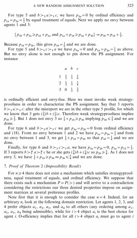
For type 5 and bo3 co3 a we have p3a=0 and p1a=p2a= 12 as above.

But no envy alone is not enough to pin down the PS assignment. Forinstance

a b c

1 12

13

16

2 12

13

16

3 0 13

23

is ordinally efficient and envy-free. Here we must invoke weak strategy-proofness in order to characterize the PS assignment. Say that 3 reportsbo3 ao3 c: after the misreport we are in the other type 5 profile, for whichwe know that 3 gets ( 2

3)b+( 13)c. Therefore weak strategyproofness implies

p3b� 23 . But 1 does not envy 3 so 1

2+p1b�p3b implying p3b� 23 and we are

done.For type 6 and bo3 ao3 c we get p3a=p2b=0 from ordinal efficiency

and (18). From no envy between 1 and 2 we have p1a=p2a= 12 and from

no envy between 1 and 3, we get 12+p1b=p3b so that p1b= 1

4 and we aredone.

Finally, for type 6 and bo3 co3 a, we have p3a=p2b=0, p1a=p12= 12 .

If 3 reports bo3* ao3* c he or she gets ( 34)b+( 1

4)c so p3b� 34 . As 1 does not

envy 3, we have 12+p1b�p3b � p3b� 3

4 and we are done.

7. Proof of Theorem 2 (Impossibility Result)

For n�4 there does not exist a mechanism which satisfies strategyproof-ness, equal treatment of equals, and ordinal efficiency. We suppose thatthere exists such a mechanism P=P(o) and will arrive to a contradictionconsidering the restrictions our three desired properties impose on assign-ment matrices at several preference profiles.

Note first that it is enough to consider the case n=4. Indeed, for anarbitrary n, look at the following domain restriction. Let agents 1, 2, 3, and4 prefer objects a1 , a2 , a3 , and a4 to all others (any ordering among a1 ,a2 , a3 , a4 being admissible), while for i>4 object ai is the best choice foragent i. O-efficiency implies that for all i>4 object ai must go to agent i


with probability 1. So the assignment problem is reduced to the first fouragents. If there exists a mechanism satisfying the premises of the theorem,its restriction to the above mentioned domain would give such a mechanismfor four agents.

In what follows, we will use the following facts.

Fact 1. Suppose that boi a, while aoj b for all j{i. Then O-efficiencyimplies pia=0. (See Step 1 in the proof of Proposition 2.) Also, let boi afor i # I, while aoj b for j � I. Then O-efficiency implies pia=0 \i # I and�orpjb=0 \ j � I.

Fact 2. Consider two orderings: R=a1oa2 o } } } oan and R$=a$1 oa$2 o } } } oa$n . Let for some k [a1 , ..., ak]=[a$1 , ..., a$k]. Let agent i changehis or her preferences from R to R$, the preferences of others being thesame (R&i ). By SP,

:k

j=1

piaj(R, R&i )= :

k

j=1

p ia$j(R$, R&i )

(of course, the same is true for the sums j=k+1 til n).

Fact. 3. Let a be the best object for everyone; then p1a=p2a=p3a=p4a= 1

4 .Indeed, it is true for an unanimous preference profile by equal treatment

of equals. Whenever agent 4 changes his or her preferences, object a beingstill his or her best, he or she has to receive p4a= 1

4 by Fact 2, while othershave to get (1& 1

4)�3= 14 by equal treatment of equals. If agent 3 changes

his or her preferences after that to be like the ordering of agent 4, then heor she still has to receive p3a= 1

4 . Hence by equal treatment of equalsp4a= 1

4 , and so again by equal treatment of equals p1, 2a= 14 . Similar

arguments apply when 1, 2 have the same orderings, while 3 and 4 havearbitrary ones (with a as the top)��we just see what happens when 3changes to be like 4 or 4 changes to be like 3��as well as in the generalcase.

Fact 4. Let exactly three agents (say, 1, 2, 3) have a as their top choice.Fact 1 gives p4a=0, while Fact 2 implies (as above) that p1a=p2a=p3a= 1

3 .We proceed by considering several preference profiles. We will write abcd

instead of aobocod, and abcd(2) if two agents in the profile have aobocod. While we refer to the agent whose preferences are listed first asagent 1, etc., we keep in mind that once we derive some restrictions on Pfor a given profile, we obtain the same restrictions for all permutations ofagents' orderings. Figure 1 records the successive facts we establish for anumber of specific profiles.


FIGURE 1

Profile 1: abcd(3), badc. By Fact 1, p4a=p4c=0 (objects a, b, thenobjects c, d ); hence p4b=p4c= 1

2 by Fact 2 (compare with profile `àbcd(4)'':p4a+p4b should not change).

Profile 2: abcd(2), abdc(2). pia= 14 by Fact 3 and by a similar argument

pib= 14 for all i. Then it follows from O-efficiency that p1, 2d=p3, 4c=0.

Indeed, p1, 2d>0 would imply p3, 4c=0 by O-efficiency, which would inturn imply p3, 4d= 1

2 (P is bistochastic!) and hence p1, 2d=0.


Profile 3: abcd(3), adbc. We have that pia= 14 by Fact 3, while by Fact

1 p4b=0 (objects b, d ) and p4c=0 (objects c, d). Thus pjb= 13 for j=1, 2, 3.

Profile 4: abcd(2), adbc, bacd (or badc!). By Fact 4, p1a=p2a=p3a= 13 ,

while p4a=0. Changing preferences of the last agent to R$=abcd gives usthe Profile 3, so by Fact 2 p4a+p4b must be the same as at that profile.Hence, p4b= 1

4+ 13&0= 7

12 .

Profile 5: abcd(3), bdac. p4a=0 by Fact 4, while p4b= 12 and p4c=0 by

Fact 2 (change of preferences of agent 4 to badc leads to Profile 1).

Profile 6: abcd(2), badc(2). When the last agent changes from badc toabcd, we obtain Profile 1. Thus p4a+p4b= 1

2 , as at Profile 1. Using equaltreatment of equals we get pia+pib=pic+p ib= 1

2 \i. Finally, using the sameargument as for Profile 2, it follows from O-efficiency that p1, 2b=p3, 4a=0,etc.

Profile 7: abcd(2), bdac(2). O-efficiency implies that in each pair( p3, 4a , p1, 2b), ( p3, 4a , p1, 2d ), and ( p3, 4c , p1, 2d) at least one probability mustbe zero. Suppose p3, 4a>0; then p1, 2b=p1, 2d=0. Hence (P is bistochastic!)p3, 4b=p3, 4d= 1

2 and so p3, 4a=0. Thus p3, 4a=0. By similar argument,p1, 2d=0, and so p1, 2a=p3, 4d= 1

2 . Before completing the assignment matrixfor this profile we need to consider another profile, namely:

Profile 8: abcd(2), bdac, badc. p3a=0 for Fact 1 (objects a, d ); p3b= 12

and p3c=0 by Fact 2 (compare with Profile 6, when agent 3 changes frombdac to badc). Look now at the last agent with preferences badc. When heor she changes to abcd we obtain Profile 5. Thus p4a+p4b= 1

3+ 16= 1

2 .When he or she changes to bdac, we obtain Profile 7. Thus p4b , p4c mustbe the same as at Profile 7. So p4b+p4c=1&(0+ 1

2)= 12 . Suppose that

p4a>0; then by O-efficiency p1, 2b=0, and so p4b= 12 ; i.e., p4a=0. Thus we

have p4a=0=p4c , and p4b= 12 .

Return to Profile 7. When the last agent changes from bdac to badc, weobtain Profile 8. So by Fact 2 p4b does not change; i.e., at the Profile 7p4b= 1

2 , p4c=0 (see the bold numbers in the matrix of Fig. 1).

Profile 9: abcd(2), bdac, adbc. By Fact 4, p1, 2, 4a= 13 , p3a=0. By Fact 1

(objects b, d) p4b=0. By Fact 2 (agent 3 changes from bdac to ba . . and weget Profile 4), p3b= 7

12 . Also by Fact 2 (agent 4 changes from adbc to bdacand we get Profile 7), p4c=0. Hence, p4d= 2

3 . Next, p1d+p2d+p3d=1&p4d= 1

3 , so p3c=1& 712&p3d�1& 7

12& 13= 1

12>0; hence by O-efficiencyp1, 2d=0.

Profile 10: abcd(2), adbc(2). pia= 14 for all i by Fact 3. When agent 3

changes from adbc to bdac, we get Profile 9. Thus by Fact 2 p3c=112 (=p4c)>0. Then by O-efficiency p1, 2d=0.


Profile 11: abcd(2), adbc, abdc. By Fact 3, pia= 14 for all i. Consider

agent 4 with preferences abdc. When he or she changes to adbc, we getProfile 10; so by Fact 2 p4c= 1

12 . When he or she changes to abcd, weget Profile 3, so by Fact 2 p4b= 1

3 . Hence, p4d= 13 . Consider now agent 3

with preferences adbc. By Fact 1 (objects b, d ), p3b=0. If agent 3 changesto abdc, we get Profile 2. So by Fact 2 p3c=0; hence p3d= 3

4 . But thenp3d+p4d= 3

4+ 13>1, which is the desired contradiction.

ACKNOWLEDGMENTS

Comments by seminar participants at Bilkent University, Bogazici University, Caltech,Northwestern University, and Universite� de Namur are gratefully acknowledged. Specialthanks to Tayfun So� nmez, Atila Abdulkadiroglu, Andy McLennan, and an anonymous referee.Moulin's research is supported by the NSF, Grant SBR9809316.

REFERENCES

1. A. Abdulkadiroglu and T. So� nmez, Random serial dictatorship and the core from randomendowments in house allocation problems, Econometrica 66 (1998), 689�701.

2. A. Abdulkadiroglu and T. So� nmez, `Òrdinal Efficiency and Dominated Sets ofAssignments,'' mimeo, University of Rochester, 1999.

3. A. Bogomolnaia and H. Moulin, `À Simple Random Assignment Problem with a UniqueSolution,'' forthcoming, Economic Theory.

4. H. Cre� s and H. Moulin, Scheduling with opting out: Improving upon random priority,Oper. Res., in press.

5. G. Demange, ``Strategyproofness in the Assignment Market Game,'' mimeo, Laboratoired'Econome� trie de Polytechnique, Paris, 1982.

6. L. Ehlers, H. Peters, and T. Storcken, ``Probabilistic Collective Decision Schemes,''mimeo, University of Maastricht, 1998.

7. D. Gale, ``College Course Assignments and Optimal Lotteries,'' mimeo, University ofCalifornia, Berkeley, 1987.

8. A. Gibbard, Straightforwardness of game forms with lotteries as outcomes, Econometrica46 (1978), 595�602.

9. W. Hofstee, Allocation by lot: A conceptual and empirical analysis, Social Sci. Inform. 29(1990), 745�763.

10. A. Hylland and R. Zeckhauser, The efficient allocation of individuals to positions, J. Polit.Econ. 91 (1979), 293�313.

11. J. Kagel and A. Roth, Eds. ``The Handbook of Experimental Economics,'' PrincetonUniversity Press, Princeton, 1995.

12. H. Leonard, Elicitation of honest preferences for the assignments of individuals topositions, J. Polit. Econ. 91 (1983), 461�479.

13. A. McLennan, `Òrdinal Efficiency and the Polyhedral Separating Hyperplane Theorem,''mimeo, University of Minnesota, 1999.

14. A. Roth and M. Sotomayor, ``Two Sided Matching: A Study in Game-Theoretic Modelingand Analysis,'' Econometric Society Monographs, Cambridge University Press, Cambridge,UK, 1990.


15. A. E. Roth and U. G. Rothblum, Truncation strategies in matching markets: In search ofadvice for participants, Econometrica 67 (1999), 21�44.

16. L. Shapley and H. Scarf, On cores and indivisibility, J. Math. Econ. 1 (1974), 23�37.17. W. Thomson and H. Varian, Theories of justice based on symmetry, in ``Social Goals and

Social Organization'' (L. Hurwicz, D. Schmeidler, and H. Sonnenschein, Eds.), CambridgeUniversity Press, Cambridge, UK, 1985.

18. H. Varian, Equity, envy and efficiency, J. Econ. Theory 9 (1974), 63�91.19. L. Zhou, On a conjecture by Gale about one-sided matching problems, J. Econ. Theory

52 (1990), 123�135.


Documents

A New Solution to the Random Assignment Problem · PDF fileJournal of Economic Theory 100, 295 328 (2001) A New Solution to the Random Assignment Problem Anna Bogomolnaia Department