Embed Size (px)
Citation preview

A NEW PI AND PID CONTROL DESIGN METHOD
AND ITS APPLICATION TO ACTIVE QUEUE
MANAGEMENT OF TCP FLOWS
a thesis
submitted to the department of electrical and
electronics engineering
and the institute of engineering and sciences
of bilkent university
in partial fulfillment of the requirements
for the degree of
master of science
By
Deniz Ustebay
June 2007


ABSTRACT
A NEW PI AND PID CONTROL DESIGN METHOD
AND ITS APPLICATION TO ACTIVE QUEUE
MANAGEMENT OF TCP FLOWS
Deniz Ustebay
M.S. in Electrical and Electronics Engineering
Supervisor: Prof. Dr. Hitay Ozbay
June 2007
PID controllers are continuing to be used in many control applications due to
their simple structures. Design of such controllers for unstable systems with time
delays is an active research area. Recently, stabilizing PI and PD controllers for
a class of unstable MIMO (multi-input multi-output) systems with input/output
delays have been investigated and allowable controller gain intervals for such
controllers have been maximized. Motivated by these studies, this thesis proposes
a new method for tuning the parameters of PI, PD and PID controllers for
integrating processes with time delays. The method is based on selecting the
centers of the maximized gain intervals as the controller gains for the purpose
of obtaining optimal controllers. As an application of this method, controllers
for AQM (Active Queue Management) of TCP (Transmission Control Protocol)
flows have been designed. AQM is a congestion control method used in computer
networks to increase link utilization with less queueing delays. The fluid flow
model of TCP’s congestion avoidance mode based on delay differential equations
supplies the mathematical background for modelling the AQM as a feedback
iii

control system and designing different control schemes accordingly. Firstly, the
proposed controller design method has been applied to AQM for the case of
time invariant time delay and secondly the method has been supported with
switching control technique to obtain optimum system performance in the case
of time varying time delay. The performance of the designed controllers for both
cases has been illustrated by packet level simulations in ns-2.
Keywords: PID control, time delay, Active Queue Management (AQM), switch-
ing control, ns-2
iv

OZET
YENI BIR PI VE PID KONTROLU TASARIMI METHODU VE
TCP AKISLARI ICIN AQM TASARIMI UYGULAMASI
Deniz Ustebay
Elektrik ve Elektronik Muhendisligi Bolumu Yuksek Lisans
Tez Yoneticisi: Prof. Dr. Hitay Ozbay
Haziran 2007
Gunumuzde bircok kontrol uygulamasında basit yapıları sayesinde PID kontrol
birimlerinin kullanımı devam etmektedir. Zaman gecikmeli kararsız sistemler icin
de bu tip kontrol birimlerinin tasarımı konusunda bircok calısma yapılmaktadır.
Bir sure once yayımlanan bir calısmada, giris ve/veya cıkıslarında zaman
gecikmesi olan bir sınıf cok girisli cok cıkıslı (MIMO) kararsız sistem icin PI ve PD
kontrol tasarımı metodu gelistirilmis ve daha sonra bu kontrol birimlerinin izin
verilen kazanc aralıklarını maksimize eden yeni bir calısma yayınlanmıstır. Bu
tezde, bahsi gecen calısmaların sonucları kullanılarak, tumlevli ve zaman gecik-
meli sistemlerde uygulanacak PI, PD ve PID kontrol birimlerinin kazanclarını
ayarlamak uzere yeni bir metot sunulmaktadır. Bu yonteme gore kontrol bir-
imlerinin kazancları izin verilen en yuksek kazanc aralıklarının merkezi olarak
alınmakta ve boylece optimal kontrol birimleri elde edilmektedir. Onerilen
yontemin bir uygulaması olarak TCP (Iletisim Kontrol Protokolu) akıslarının
AQM (Etkin Kuyruk Yonetimi) problemi icin kontrol birimleri tasarlandı. Etkin
kuyruk yonetimi, bilgisayar aglarında kullanılan bir sıkısıklıgı giderici kontrol
yontemi olup amacı kuyrukta bekleme gecikmelerini azaltmak ve baglantıların
kullanım oranını artırmaktır. Daha once yapılan calısmalarda, sıkısıklıktan
v

kacınma modunda calısan TCP’nin turevsel denklemelere dayalı sıvı akıs modeli
kullanılarak AQM bir geri besleme sistemi olarak modellenmistir. Bu model kul-
lanılarak uygun kontrol birimleri tasarlandı. Onerilen kontrol metodu oncelikle
zamanla degismeyen zaman gecikmesi durumu icin AQM’ye uygulandı. Ikinci
olarak, metot anahtarlamalı kontrol yontemi de kullanılarak zamanla degisen
zaman gecikmeli duruma uygulandı. Her iki durum icin de gelistirilen kon-
trol birimlerinin performansları ns-2 platformunda paket duzeyinde benzetimlerle
gosterildi.
Anahtar Kelimeler: PID kontrol, zaman gecikmesi, Etkin Kuyruk Yonetimi
(AQM), anahtarlamalı kontrol, ns-2
vi

ACKNOWLEDGMENTS
I gratefully thank my supervisor Prof. Dr. Hitay Ozbay for his enthusiasm,
encouragement, patience, and never ending guidance. Working under his su-
pervision has been a great pleasure and honor. I have learned a lot from him
and his cheerful attitude has always been a good reason to cheer up. I also
thank to the members of my thesis committee Prof. Dr. Omer Morgul and
Asst. Prof. Dr. Ibrahim Korpeoglu for their support.
I would like to thank my friend Ozlem Guler for being my project mate during
graduate courses and for always being by my side. Sengor Altıngovde is one of
the most inspiring and funny friends ever and I thank him for being the source
of humor during the creation of this thesis. Many thanks go to Rohat Melik, he
has helped me with every little detail in these last few months. I also thank my
office mates Zeynep Yucel and Mehmet Kok. The friendly atmosphere that we
have created in EA227 is to be missed a lot.
Finally, my thanks go to my family. Their efforts beginning form the first
day of my life and their unlimited support made everything possible.
vii

Contents
1 Introduction 1
2 PI, PD and PID Control for Integrating Systems with Time
Delay 5
2.1 PD Controller . . . . . . . . . . . . . . . . . . . . . . . . . . . . . 6
2.2 PI Controller . . . . . . . . . . . . . . . . . . . . . . . . . . . . . 8
2.3 PID Controller . . . . . . . . . . . . . . . . . . . . . . . . . . . . 10
2.4 Switching Control . . . . . . . . . . . . . . . . . . . . . . . . . . . 11
3 Application to AQM 12
3.1 Mathematical Model of AQM Supporting TCP Flows . . . . . . . 12
3.1.1 Linearization . . . . . . . . . . . . . . . . . . . . . . . . . 14
3.2 Application of the proposed control
methods . . . . . . . . . . . . . . . . . . . . . . . . . . . . . . . . 18
3.2.1 An alternative PID controller design . . . . . . . . . . . . 19
3.2.2 Switching Control . . . . . . . . . . . . . . . . . . . . . . . 20
viii

3.2.3 Digital implementation of the controllers . . . . . . . . . . 22
4 Simulation Results 24
4.1 Simulation results for the nominal network parameters . . . . . . 24
4.2 Robustness to uncertainties in the network parameters . . . . . . 27
4.3 Switching Control . . . . . . . . . . . . . . . . . . . . . . . . . . . 29
5 Conclusions 37
A ns-2 C++ function adapted for PID controller 39
B ns-2 tcl code (PI controller case) 41
ix

List of Figures
1.1 Delay representation . . . . . . . . . . . . . . . . . . . . . . . . . 2
2.1 Feedback system . . . . . . . . . . . . . . . . . . . . . . . . . . . 6
3.1 RED: Probability of packet marking vs. average queue size . . . . 16
3.2 Linearized Feedback System . . . . . . . . . . . . . . . . . . . . . 18
3.3 Γ(ω)/Ro versus ω for f(s)= e−Ros
1+Ros. . . . . . . . . . . . . . . . . . 19
3.4 Γ(ω)/Ro versus ω for fo(s)=e−Ros(8θs+1)
(KRos+1)(Ros+1). . . . . . . . . . . . . 20
3.5 RTT . . . . . . . . . . . . . . . . . . . . . . . . . . . . . . . . . . 21
4.1 Network Topology . . . . . . . . . . . . . . . . . . . . . . . . . . 25
4.2 ns-2 simulations: queue length vs time. . . . . . . . . . . . . . . 26
4.3 ns-2 simulations: queue length vs time for c=1563 packets/sec. . 29
4.4 ns-2 simulations: queue length vs time for N=40 TCP flows. . . . 30
4.5 ns-2 simulations: queue length vs time for RTT=0.4 sec. . . . . . 31
4.6 Mean and standard deviation of queue length under load variations 32
x

4.7 Errors under load variations . . . . . . . . . . . . . . . . . . . . . 32
4.8 Errors under load variations . . . . . . . . . . . . . . . . . . . . . 32
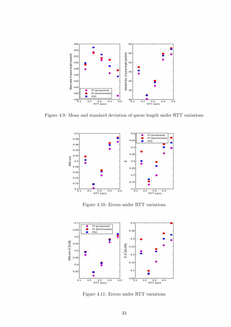
4.9 Mean and standard deviation of queue length under RTT variations 33
4.10 Errors under RTT variations . . . . . . . . . . . . . . . . . . . . . 33
4.11 Errors under RTT variations . . . . . . . . . . . . . . . . . . . . . 33
4.12 Mean and standard deviation of queue length under capacity vari-
ations . . . . . . . . . . . . . . . . . . . . . . . . . . . . . . . . . 34
4.13 Errors under capacity variations . . . . . . . . . . . . . . . . . . . 34
4.14 Errors under capacity variations . . . . . . . . . . . . . . . . . . . 34
4.15 ns-2 simulations: (a) RTT1 (b) single controller, Kpi0 (c) single
controller, Kpi1 (d) single controller, Kpi2 (e) two switching con-
trollers, Kpi1 and Kpi2, (f) N=16 switching controllers . . . . . . . 35
4.16 ns-2 simulations: (a) RTT2 (b) single controller, Kpi0 (c) single
controller, Kpi1 (d) single controller, Kpi2 (e) two switching con-
trollers, Kpi1 and Kpi2, (f) N=16 switching controllers . . . . . . . 36
xi

List of Tables
4.1 The analysis of simulation results . . . . . . . . . . . . . . . . . . 26
4.2 The analysis of simulation results for c=1563 packets/sec . . . . . 28
4.3 The analysis of simulation results for N=40 TCP flows . . . . . . 28
4.4 The analysis of simulation results for RTT=0.4 sec . . . . . . . . 28
4.5 The analysis of simulation results for RTT1 . . . . . . . . . . . . . 35
4.6 The analysis of simulation results for RTT2 . . . . . . . . . . . . . 36
xii

To my parents, Sultan and Fettah

Chapter 1
Introduction
Proportional-Integral-Derivative (PID) controllers are widely used in various en-
gineering applications since they are easy to implement using low storage mem-
ory, their computational complexity is low and they are applicable to most control
systems, [1], [6]. PID controllers may not provide optimal control in many situa-
tions but they have proved their usefulness in providing satisfactory control with
the advantages above. In fact, today more than half of the industrial controllers
utilize PID or modified PID control schemes, [16].
In the most general form PID controllers are second order systems
Kpid(s) = Kp +Ki
s+ Kds (1.1)
where Kp is the proportional gain, Ki is the integral gain and, Kd is the derivative
gain. Furthermore, (1.1) with Kd=0 is a PI controller and (1.1) with Ki=0 is a
PD controller.
The main issue in PID control design is the “optimal” tuning of the gains,
Kp, Ki, Kd and many different types of tuning guidelines have been proposed in
the literature. Some current techniques for PID controller design include the
Ziegler-Nichols tuning methods, internal model controller (IMC) based tuning
1

u(t−T)u(t) Delay T
Figure 1.1: Delay representation
methods and dominant pole design (Cohen-Coon method). A comprehensive
survey on PID controller design methods can be found in [1].
In this study we consider integrating systems with time delays (i.e. the plant
contains an integrator, a time delay, and possibly other stable terms). Delays are
present in a system if a signal or a physical variable originating form one part of
the system becomes available in another part of the system after a lapse of time.
The block diagram of a delay element is given in Figure (1.1) and in Laplace
domain this delay is represented as e−Ts. Many problems in control engineering
involve time delays such as chemical processes, aerodynamics and communication
networks. Tuning of PID controllers for this type of unstable time delay systems
is an active research area, see [13], [20], [24] and the references therein.
In a recent study, stabilizing PID controllers are obtained for a class of MIMO
(multi-input multi-output) unstable plants with delays in the input and output
channels, [17]. Using the results of this study resilient PI (Proportional-Integral)
and PD (Proportional-Derivative) controllers with largest allowable controller
gain intervals are investigated for plants with at most two unstable poles, [7].
Maximization of the controller gain intervals is an important problem since this
way the sensitivity of the closed loop stability to perturbations in the controller
parameters can be minimized. In this thesis, the results of [17] and [7] are used to
obtain the largest allowable gain intervals for a SISO (single-input single-output)
plant with a given set of nominal plant parameters and the center of these max-
imized intervals is selected as the optimal gains of the controllers. Controllers
with perturbed gains can be seen as “optimal” controllers for plants with per-
turbed nominal parameters. So, the controllers proposed here are expected to
2

work for a wide range of plant parameters. Controllers using this method can be
applied to integrating time delay systems appearing in data flow control in com-
puter networks, target tracking problems in robotics applications, and material
transport systems encountered in process control.
In this study, proposed PID control method is applied to AQM schemes sup-
porting TCP flows. TCP is currently the dominant transport protocol used in
the Internet and with the addition of AQM, routers are able to detect congestion
before the queues overflow. Congestion occurs in a network when the demand
for the link bandwidth is higher than the available capacity of the resource, [23].
When some of the links are congested in a network, buffers at the routers over-
flow and any new incoming packets are dropped or lost. This situation leads to
long return-trip-times (RTT), i.e. delays, and may even result in an instability
in the network (e.g. congestion collapse in the Internet), [5]. On the other hand,
having an empty queue at a buffer means that the link capacity is not fully used,
i.e. network resources are under-utilized in this case. Therefore, the goal of AQM
is to keep the queue size at the buffers at a certain desired level. For this pur-
pose, most AQM schemes mark the Explicit Congestion Notification (ECN) bit
of the packets passing through the link according to a certain rule, [21]. In early
AQM methods, such as RED (Random Early Detection) [4] and REM (Random
Exponential Marking) [2], packet marking probability (control signal) is a static
function of the queue (or average queue) size. In [11], [14] mathematical mod-
els of AQM schemes supporting TCP flows have been proposed and with the
help of these models a control-theory based approach to analyze or design AQM
schemes has been possible. First attempts to design a dynamic controller appear
in [8, 9], where the authors use the fluid model of the TCP flows developed in
[14] to design a PI controller. This AQM scheme is currently implemented in
ns-2, [15] and in [9] it is shown that it performs better than RED. Therefore, PI
controller of [9] will be taken as the “benchmark” design for comparisons with
the alternative AQM controller tuning method proposed here.
3

Different schemes of AQM deploying control theory methods have been pro-
posed in the literature. In [12], a rate based controller method called adaptive
virtual queue (AVQ) has been proposed. A PID controller has been designed
for AQM with time domain analysis methods in [22]. Another rate based con-
trol mechanism which is called virtual rate control (VRC) has been proposed
in [19] and in fact it is just a PID controller. In [18], an H∞ controller has
been designed and later in [26], H∞ performance of the designed controller with
respect to uncertainty bound of RTT has been analyzed. Another robust H∞
based AQM control scheme (RHC) has been introduced in [3] to maintain queue
stabilization in the presence of variations of the network parameters. In [25]
a variable structure sliding mode controller based AQM scheme has been de-
signed for better performance in terms of packet loss ratio, link utilization and
queue fluctuation. With the exception of [26] , where H∞ based AQM techniques
are used, the papers mentioned above do not consider time varying propagation
delays, which may occur due to changes in the communication channels. [26]
proposes switching among a set of robust controllers designed at small operating
ranges for better performance than a single controller for the whole range of time
delay. However the proposed H∞ control method of [26] is relatively complicated
to implement in real networks. Therefore in this thesis switching is done among
PI controllers since they are much simpler and easy to implement.
Remaining parts of the thesis are organized as follows. Details of the con-
troller parameter tuning is given in Section 2. Application of this tuning method
to the AQM problem can be found in Section 3 whereas the simulation results
of this application along with the comparisons of the benchmark design with the
proposed design can be found in 4. Concluding remarks are made in Section 5.
4

Chapter 2
PI, PD and PID Control for
Integrating Systems with Time
Delay
In a recent study [7], existence of stabilizing PID (Proportional-Integral-
Derivative) controllers is shown for LTI (linear time-invariant) MIMO (multi-
input multi-output) unstable plants with possibly uncertain time delays in the
input and output channels. For plants with one or two unstable poles the pa-
rameters of these PID controllers are explicitly formulated from a small gain
argument. Using the results of this study, stabilizing PI (Proportional-Integral)
and PD (Proportional-Derivative) controllers with largest allowable gain inter-
vals are investigated in [17] for plants with only one unstable pole. Using the
results of these two studies we propose a new method for tuning the parameters
of PI and PID controllers for integrating processes with time delays.
Consider the unity feedback system in the Figure 2.1. The transfer function
of the plant is in the form
GΛ(s) =Ko
se−hsg(s), h > 0 (2.1)
5

yyref C
e u
v
G Λ
Figure 2.1: Feedback system
where g(s) is an arbitrary stable rational transfer function satisfying g(0) = 1
and therefore the only unstable pole of the plant is at s=0. For notational
convenience we define
f(s) := e−hsg(s) (2.2)
and let
G(s) =Ko
sg(s) (2.3)
be the finite dimensional part of the plant. A coprime factorization of G(s)
is in the form G(s) = X(s)Y (s)−1 with X(0) = sG(s) |s=0 6= 0. In this case,
Y (s) = s/(as + 1), for any a > 0, and since g(0) = 1, we have X(0) = Ko.
2.1 PD Controller
In [7] it is shown that a PD controller in the form
Kpd(s) = αX(0)−1(1 + Kds) (2.4)
stabilizes the feedback system of Figure 2.1 for any α ∈ R satisfying
0 < α < ‖ΦΛ‖−1∞ = (sup
ω‖ΦΛ(jω)‖)−1 (2.5)
where
ΦΛ :=GΛ(s)Kpd(s)
α− s. (2.6)
This overall gain interval is maximized in [17] for the purpose of obtaining a
resilient controller. Maximizing ‖ΦΛ‖−1∞ is equivalent to minimizing
µ := ‖ΦΛ‖∞ = ‖s−1(f(s)(1 + Kds)− 1)‖∞ (2.7)
6

For Kd being the free parameter this problem reduces to finding a Kd ∈ R such
that
µ = ‖f(s)− 1
s+ Kdf(s)‖∞ (2.8)
is minimized. Let the optimal solution be Kd, opt. This is a single parameter
scalar H∞ norm minimization problem which can be solved numerically with
brute force search. The following algorithm steps will find a solution:
1. Choose candidate values of Kd = K1, ..., KN and frequency values
ω = ω1, ..., ωM . The optimization will be done over the K values whereas norm
will be calculated over the ω values.
2. For k = 1, ..., N and l = 1, ..., M compute
Ψ(Kk, ωl) := ‖f(jωl)− 1
jωl
+ Kkf(jωl)‖. (2.9)
3. Define µ(Kk)=maxωlΨ(Kk, ωl).
4. Optimal Kd is Kd, opt=arg minKkµ(Kk).
One can find a solution to (2.8) with this algorithm but that solution will be
sensitive to the number of grid points chosen for K and ω. Therefore, a direct
computation of the optimal solution will be more useful.
A closed form expression of the solution is given in Proposition 2 of [17] as:
Let f(s) = g(s)e −hs, with g ∈ H∞, g(0) = 1,and h > 0. Also let ρ(ω) := |f(jω)|and φ(ω) := ∠f(jω) being the magnitude and phase functions of f(jω) and
η(ω) :=
∣∣∣∣ρ(ω)− cos(φ(ω))
ω
∣∣∣∣ (2.10)
being a function with maximum, ηo, which is attained at a single frequency ωo,
in other words,
ηo := maxω
∣∣∣∣ρ(ω)− cos(φ(ω))
ω
∣∣∣∣ = η(ωo).
Then, the optimal solution of
Kd, opt = arg minKd∈R
‖f(s)− 1
s+ Kdf(s)‖∞ (2.11)
7

is given by
Kd, opt = − sin(φ(ωo))
ωo ρ(ωo)(2.12)
if
Γ(ω) := η2o − η2(ω)− |Ko − Kd, opt(ω)|2ρ2(ω) ≥ 0 ∀ω (2.13)
is satisfied. Note that to find Kd, opt we have to just find ωo numerically whereas
the algorithm given above requiring two dimensional search is much complicated.
Therefore (2.12) is the optimal solution of (2.8) which maximizes the lower
bound for ‖ΦΛ‖−1∞ and the corresponding maximal lower bound for ‖ΦΛ‖−1
∞ is
found as 1/ηo.
We propose to take Kd, opt as the derivative gain and the center of the max-
imum allowable overall gain interval as the overall gain, i.e. α=1/2ηo and the
resulting PD controller is in the form
Kpd(s) =1
2ηo
(1
Ko
+ Kds). (2.14)
The above PD controller design technique is valid for all plants in the form
(2.1) where g(s) can be any stable rational transfer function satisfying g(0) = 0,
with one caveat: one has to check that the corresponding η has a single maximum.
For a first order strictly proper g(s) (as in the AQM problem to be shown) this
is automatically satisfied.
2.2 PI Controller
According to [7] a PI controller in the form
Kpi(s) = αX(0)−1(1 +γ
s) (2.15)
stabilizes the feedback system in Figure 1 for any α ∈ R satisfying (2.5) with
Kd = 0 and any γ ∈ R satisfying
0 < γ < γmax := ‖αsf(s)(1 + α
sf(s))−1 − 1
s‖−1∞ . (2.16)
8

For such a PI controller, the maximum integral action gain interval is studied for
fixed overall controller gain in [17]. First the function θ := ‖f(s)−1s‖∞ is defined
and then (2.5) can be rewritten as
0 < α < θ−1 (2.17)
and the lower bound for γmax is found as
γ∗ = α(1− αθ) ≤ γmax . (2.18)
With straightforward calculation it can be shown that the optimal α maximizing
this lower bound is α∗ = 1/2θ and the maximal γ∗ corresponding to this optimal
α is γ∗,max = α∗/2.
To make the controller robustly stable with respect to largest perturbations
in the controller parameters we propose to choose controller’s proportional gain
as α∗ and integral gain as γ∗,max/2, which is the center of the maximal interval.
The resulting PI controller is in the form
Kpi(s) =1
2θ
1
Ko
(1 +1
8θs). (2.19)
It should be noted that, while we tried to maximize the upper bound of the
overall controller gain, the optimal overall gain came up as the center of the
overall controller gain interval. Therefore both the overall controller gain and
integral gain of the optimal PI controller are at the center of their corresponding
intervals.
The computation of (2.19) above is rather simplified thanks to conservatism
introduced by (2.18). In fact, γ−1max is a function of α:
γ−1max = sup
ω
∣∣∣∣1
jω + αf(jω)
∣∣∣∣ =: Q(α).
This norm should be calculated for every α in the interval 0 < α < 1/θ. Then
γ−1max could be chosen as the minimum of Q(α). However, this method requires
9

M ∗ N calculations for M being the ω grid points for H∞ norm computation
and N being the α grid points. Using (2.18) we skip the H∞ norm computation
for every fixed α. The conservatism introduced by (2.18) is currently under
investigation.
2.3 PID Controller
A PID controller can be obtained from the product of PI and PD controllers,
Kpid(s) = (Kp1 +Ki
s)(Kp2 + Kds) = (Kp1Kp2 + KiKd) +
KiKp2
s+ Kp1Kds.
So, we will first design a PD controller, then design a PI controller for the PD
controlled open loop plant. The transfer function of the PD controlled plant is
GΛ(s)Kpd(s) =Ko
se−hsg(s)
1
2ηo
(1
Ko
+ Kds) =:1
2ηo
e−hsgo(s)
s
with
go(s) := g(s) (1 + KoKds).
Let’s define
θo := ‖go(s)− 1
s‖∞ (2.20)
such that a PI controller is formed with the method explained in Section 2.2:
Kpi(s) =1
2θo
2ηo (1 +1
8θos). (2.21)
So, the PID controller is
Kpid(s) =(1 + KoKds)
16Koθ2o
(1 + 8θos)
s. (2.22)
It is also possible to obtain a PID controller by first designing a PI controller
and then designing a PD controller for the PI controlled open loop plant. Such
a plant will have two poles at zero, one from the original plant (2.1) and one
from the PI controller (2.19) however the method proposed in [17] is valid for
10

plants with only one unstable pole. Therefore, we will not not use this method
for designing a PID controller for (2.1). On the other hand, in the application
problem (AQM) we will find an alternative to overcome this obstacle, see Section
(3.2.1).
2.4 Switching Control
For real systems with time varying time delays,the above controller design meth-
ods can be further improved. In [26], it was proposed to divide the range of time
delay into a number of smaller regions and designing controllers for each of these
regions. Then, while the time delay varies, switching between these controllers
accordingly is proposed to give better results than using a single controller de-
signed for the entire region of time delay. In that study, the application was done
for two switching controllers, here we increase the number of controllers and we
apply the idea to our proposed controllers. This method is detailed in Section
3.2.2 for the studied application problem.
11

Chapter 3
Application to AQM
3.1 Mathematical Model of AQM Supporting
TCP Flows
This thesis considers a network configuration consisting of a single bottleneck
link supporting N TCP flows and the routers mark the ECN bits of packets
to inform the TCP sources of congestion as proposed in [21]. The dynamical
model of TCP was developed using stochastic differential equation analysis and
fluid flow approximation in [14]. In this study a simplified version of this model
which was introduced in [9] is used. The model provides means for analysis and
design for TCP in congestion avoidance mode only, thus ignores the slow-start
and timeout mechanisms of TCP. In this model TCP dynamics are represented
with the following nonlinear differential, time-delayed equations:
W (t) =1
R(t)− W (t) W (t−R(t))
2 R(t−R(t))p(t−R(t)) (3.1)
q(t) = N(t)W (t)
R(t)− c(t) when q(t) > 0 (3.2)
where x(t) denotes time derivative and
12

W : average TCP window size (packets),
q : average queue length (packets),
R : round-trip time (seconds),
c : link capacity (packets),
N : number of TCP flows (i.e. load),
p : probability of packet mark.
Here, RTT (total delay in the feedback path) is expressed by
R(t) = Tp(t) +q(t)
c(t)(3.3)
where Tp(t) is the propagation delay and obviously, q(t)/c(t) is the queueing
delay. Note that in this study both time invariant and time varying round trip
time cases are considered. For the later case, the assumption is that the variations
of Tp(t) are slow compared to the variations of q(t)/c(t), but the magnitude of
the variations of the propagation delay is larger than the variations of queueing
delay. Therefore, the time variation in RTT will be taken to be due the variation
in the propagation delay.
Equation 3.1 specifies the TCP window dynamic in congestion avoidance
mode incorporating the additive increase and multiplicative decrease (AIMD)
behavior of TCP. In the right side of this equation, the 1/R term represents the
increase in the sending rate when no congestion is detected and the W/2 term
models the decrease in the sending rate when congestion is detected, i.e. packets
are marked with probability p.
Likewise, Equation 3.2 models the queue length dynamic as the difference
between incoming flow rate and outgoing flow rate (i.e. link capacity). It is
possible to use these equations to describe TCP as a feedback control system,
where p is the control input generated by a feedback from q, i.e.
p = K(q) (3.4)
13

where K is the feedback control operator. Clearly, the above system is nonlinear
and it depends on an implicit function R(t − R(t)). In general, ”optimal” con-
trollers for such nonlinear dynamical systems are difficult to obtain. Typically
the system is linearized around an equilibrium point using small signal analysis.
3.1.1 Linearization
To perform linearization on equations (3.1) and (3.2), we first assume that the
link capacity and the number of TCP sessions are constant, c(t) = c and N(t) =
N , as in [9]. The following equations should be satisfied for the equilibrium point:
W = 0 =⇒ Wo2po
2= 1 (3.5)
q = 0 =⇒ WoN
Ro
= c. (3.6)
Then, given the set of network parameters ζ.= (N,C, Tp), the operating point is
defined by the solution (Ro,Wo, po) of the following equations:
Ro =qo
c+ Tp (3.7)
Wo =RoC
N(3.8)
po =2
W 2o
(3.9)
for a desired equilibrium queue size qo. Additionally, Wo ∈ (0, W ), qo ∈ (0, q),
po ∈ (0, 1) should also be satisfied where W is the maximum window size and
q is the buffer capacity. We also assume that the time delay element R(t) in
(t− R(t)) is constant and equal to Ro. Then, the equations (3.1) and (3.2) can
be rewritten as:
W (t) =1
q(t)c
+ Tp
− W (t)
2
W (t−Ro)q(t−Ro)
c+ Tp
p(t−Ro) (3.10)
q(t) = N(t)W (t)
R(t)− c(t) when q(t) > 0 (3.11)
14

In order to linearize these two equations we first define
f(W,Wd, q, qd, pd).=
1qc+ Tp
− W Wd
2 (qd
c+ Tp)
pd (3.12)
g(W, q).=
Nqc+ Tp
W − c (3.13)
where Wd.= W (t−Ro), qd
.= q(t−Ro), pd
.= p(t−Ro) are the delayed variables.
Using the operating point relationships (3.5) and (3.6), the partial derivatives of
f and g at the operating point are found as:
∂f
∂W= −Wo po
2Ro
= − 1
2Ro
= − 1
WoRo
= − N
R2oC
∂f
∂Wd
=∂f
∂Wd
= − N
R2oC
∂f
∂q= − 1
R2oc
∂f
∂qd
= −W 2o po
2R2o
(−1
c) =
1
R2oc
∂f
∂pd
= −W 2o
2Ro
= −Roc2
2N2
∂g
∂q= −NWo
R2oc
= − 1
Ro
∂g
∂W= −N
Ro
.
We then obtain
δW (t) = δW (t)∂f
∂W+δW (t−Ro)
∂f
∂Wd
+δq(t)∂f
∂q+δq(t−Ro)
∂f
∂qd
+δp(t−Ro)∂f
∂pd
= − N
R2oC
(δW (t)+δW (t−Ro))− 1
R2oc
(δq(t)−δq(t−Ro)−Roc2
2N2δp(t−Ro) (3.14)
δq(t) = δW (t)∂g
∂W+ δq(t)
∂g
∂q=
N
Ro
δW (t)− 1
Ro
δq(t) (3.15)
with
δW = W −Wo,
δq = q − qo,
δp = p− po
representing the small signal variables.
15

We will now consider the Random Early Detection (RED), [4], algorithm
as the AQM scheme, and show that qo is an equilibrium point. RED takes an
average measure of the router’s queue length and randomly marks ECN bits of
packets. The averaging which is achieved by a low-pass filter, is for eliminating
the effects of restarts and time-outs on the feedback signal. The randomness
on the other hand, is meant to overcome flow synchronization, [9]. The packet
marking probability as a function of average queue size is illustrated in Fig. 3.1.
p
1
max
qmin qmax
p(t)
averagequeue
Figure 3.1: RED: Probability of packet marking vs. average queue size
As shown in the figure, packets are marked when the average queue size is between
maximum and minimum threshold values, qmax andqmin, with probability
p(t) = (pmax
qmax − qmin
)(qav(t)− qmin). (3.16)
The goal of RED is keeping qav(t) near its equilibrium point between qmax and
qmin. At equilibrium qavo = qo and the slope in Fig. 3.1 is
L.=
pmax
qmax − qmin
. (3.17)
Then the probability of packet mark satisfies:
po =pmax
qmax − qmin
qo − pmax
qmax − qmin
qmin.= αqo − β. (3.18)
Using equations (3.7), (3.8) and, (3.9)
po =2
W 2o
=2N2
c2R2o
=2N2
qo + cTp2 = αqo − β (3.19)
16

is found. Then qo should satisfy:
αqo(qo + cTp)2 − β(qo + cTp)
2 − 2N2 = 0 (3.20)
q3o + (2cTp − β
α)q2
o + cTp(cTp − 2β
α)qo − (
β
α)c2T 2
p −2N
α= 0. (3.21)
From (3.18) it is obvious that
β
α= qmin. (3.22)
Assuming qmin = 0, equation (3.21) can be rewritten as
q3o + 2cTpq
2o + c2T 2
p qo − 2N
L= 0. (3.23)
Let’s write the Routh Hurwitz array for this equation:
s3 1 c2T 2p
s2 2cTp − 2N2L
s X1 − 2N2L
From the array it is found that: X =2c3T 3
p +2N2L
2cTp. However, independent
of the sign of X , there is always one sign change in the first row of the array.
Therefore, there is always one root of qo in the right half plane. This proves that
the equilibrium point of equations (3.1) and (3.2) exits and is unique.
Turning back to the linearization problem, the differential equation for the
low-pass filter of RED is
qav(t) = −aqav(t) + aq(t) (3.24)
and with simplifying (3.1.1) as:
δW ∼= − 2N
R2oC
δW − Roc2
2N2δp (3.25)
we obtain a block diagram representation of the linearized TCP dynamics for
RED with separated window and queue dynamics as in Figure (3.2). The transfer
17

R
2NoC
2
N
Ro
2C
s+
NRo
1Ro
s+ as+
a
e-sRo L
TCP window dynamicqueue dynamic
low-pass filter
Delay (RTT)
dp(t-Ro) dW dq dqav
dp(t)
2
Figure 3.2: Linearized Feedback System
function Gpq(s) from the control input δp to the output to be regulated δq can
be obtained as:
Gpq(s) = e−Ros Roco K
Ros + K−1
1
Ros + 1, K =
Roco
2No
. (3.26)
In this feedback system, the effect of the RED is the constant gain controller L =
pmax
qmax−qminand the main idea behind designing controllers for AQM is designing
controllers and replacing L with these controllers.
3.2 Application of the proposed control
methods
With the assumption of K À 1, the “plant” (3.26) is approximately in the form
(2.1) with Ko := coK, h = Ro and g(s) = (1 + Ros)−1. Hence, we can apply the
technique proposed of Section 2 to design PI, PD and PID controllers. However,
for the design of PD controller one should not forget to check whether condition
(2.13) is satisfied. Figure 3.3 shows that it is satisfied for the plant model of
AQM.
18

10−1
100
101
102
103
−0.1
0
0.1
0.2
0.3
0.4
ω
Γ(ω)/Ro
Ro=0.48 sec.
Ro=0.4 sec.
Ro=0.32 sec.
Ro=0.24 sec.
Ro=0.16 sec.
Figure 3.3: Γ(ω)/Ro versus ω for f(s)= e−Ros
1+Ros
3.2.1 An alternative PID controller design
As addressed at the end of Section 2.3 there is a second possible PID control
design method with first designing a PI controller and then designing a PD
controller for the PI controlled plant. This PID controller design method is not
applicable to plant (2.1) since the PI controlled plant has two unstable poles and
the PD control design method is valid for those with only one unstable pole.
However, for the special case of (3.26) we propose an alternative approach. We
first design the PI controller as proposed and after that we release the assumption
of K À 1. Then the transfer function of the PI controlled plant becomes
Gpq(s)Kpi(s) =KRo
16θ2
(8θs + 1)e−Ros
s(KRos + 1)(Ros + 1)=:
KRo
16θ2
go(s)
s(3.27)
with only one unstable pole which comes from the PI controller. Hence the PD
design method of Section 2.1 is valid for (3.27). Note that, Figure 3.4 shows that
condition (2.13) is satisfied for the PI controlled plant.
For designing the PD controller, first define fν = e−Rosgo(s) then, set ρν(ω) :=
|fν(jω)| and φν(ω) := ∠fν(jω) as the new magnitude and phase functions. Then
set ην(ω) := |ρν(ω)−cos(φν(ω))ω
|. Assume that ην(ω) has a maximum, ην,o, which is
19

10−1
100
101
102
103
−5
0
5
10
15
20
25
30
35
ω
Ro=0.16 sec.
Ro=0.24 sec.
Ro=0.32 sec.
Ro=0.4 sec.
Ro=0.48 sec.
Γ(ω)/Ro
Figure 3.4: Γ(ω)/Ro versus ω for fo(s)=e−Ros(8θs+1)
(KRos+1)(Ros+1)
attained at a single frequency ων,o. With this assumption define
Kdν := −sin(φν(ων,o))
ων,o ρν(ων,o).
Then the PD controller is
Kν,pd(s) =1
2ην,o
(16θ2
KRo
+ Kdνs).
Thus the overall PID controller for the plant (3.26) is the product of Kpi(s) and
Kν,pd(s), that is,
Kpid(s) =(16θ2 + Kdνs)
32ην,ocoRoK2
(1 + 8θs)
s. (3.28)
3.2.2 Switching Control
In computer networks RTT is probably time varying or uncertain and for better
performance, in [26], switching among a set of robust controllers was proposed.
In this section we use this method to design PI controllers for smaller operating
ranges of RTT and switch among them accordingly for the case of known RTT
variation. Note that, we only explain the method for PI controller case but it
can be easily applied to PD, PID or any other controller. However, we will give
20

results in Section 4.3 only for switching PI controllers since they give satisfactory
results with less parameter computation. Ro +�RRo ��R R1 R2RoFigure 3.5: RTT
For the case shown in Fig. 3.5, the nominal value of RTT is Ro and we assume
that RTT takes values between Ro − ∆R and Ro + ∆R. If we are to design a
single PI controller for this plant we can assume
(i) the plant is nominal, let R = Ro, and implement Kpi0,
(ii) for Ro −∆R < RTT < Ro, let R = R1 = Ro − ∆R2
and implement Kpi1
(iii) for Ro < RTT < Ro + ∆R, let R = R2 = Ro + ∆R2
and implement Kpi2.
As the designed PI controllers are robust to the changes in RTT (to be shown
in Section 4.2), these three controllers are expected to have good performance in
the neighborhood of RTT values they are designed for. In this thesis, we illustrate
that it is possible to improve the performance in the case of time varying RTT
by applying switching control. Two different configurations are investigated:
a) Using two of the PI controllers above, we perform mid-point switching. When
RTT is in [Ro−∆R,Ro] interval Kpi1 is active and when RTT is in [Ro, Ro +∆R]
interval Kpi2 is active.
b) Instead of dividing [Ro − ∆R,Ro + ∆R] interval into two, we divide it into
N À 1 intervals. Therefore, we design N different PI controllers for each of these
intervals and as RTT varies among these intervals, the controller parameters
switch accordingly.
The switching mentioned above is actually mid-point switching since RTT is
assumed to be varying slowly, free of sudden large deviations. It should be noted
that, for a more frequently changing time delay case (i.e., chattering), hysteresis
switching may be beneficial.
21

3.2.3 Digital implementation of the controllers
When implementing these controllers in discrete time we need to convert the
differential equations into difference equations, there are several ways to do this,
see e.g. [10]. In [8] a method for the digital implementation of the PI controller
for ns-2 implementation is given. We slightly modify this method and also apply
it to the PID controller case. For digital implementation, z-transform of the
controller transfer function is calculated without any approximation and a proper
sampling frequency, fs, is chosen. It is advised to choose fs as 10-20 times the
loop bandwidth. In our case, the loop bandwidth is between 0.1-0.3 Hz, so we
choose fs = 4 Hz.
The PI controller transfer function is in the form (1.1) with Kd = 0, and in
z-domain it becomes:
Kpi(z) =a− bz−1
1− z−1(3.29)
where
a = Kp (3.30)
b = Kp −KiTs (3.31)
and, Ts = 1/fs. Note that, since Kpi(z) is the transfer function from δq(t) to
δp(t), (3.1), and assuming po is equal to 0, we can write:
p(z)
δq(z)=
a− bz−1
1− z−1. (3.32)
This transfer function can be converted to the following difference equation for
t = kTs:
p(kTs) = aδq(kTs)− bδq((k − 1)Ts) + p((k − 1)Ts) (3.33)
The digital implementation of this difference equation is done with the following
pseudo code:
p = a(q − qo)− b(qold − qo) + pold (3.34)
22

pold = p (3.35)
qold = q (3.36)
Similarly the PID controller (1.1) in z-domain can be given as:
Kpid(z) =a0 + a1z
−1 + a2z−2
b0 + b1z−1 + b2z−2(3.37)
where
a0 = Kp + Kd (3.38)
a1 = −Kp − 2Kd + KiTs (3.39)
a2 = Kd (3.40)
b0 = 1 (3.41)
b1 = −1 (3.42)
b2 = 0 (3.43)
and, Ts = 1/fs. As in the above case, we can write
p(z)
δq(z)=
a0 + a1z−1 + a2z
−2
b0 + b1z−1 + b2z−2. (3.44)
and for t = kTs the difference equation is
p(kTs)+b1p((k−1)Ts)+b2p((k−2)Ts) = a0δq(kTs)−a1δq((k−1)Ts)+a2δq((k−2)Ts)
(3.45)
The digital implementation of this difference equation is done with the following
pseudo code:
p = a0(q − qo) + a1(qold − qo) + a2(qelder − qo)− b1pold − b2pelder(3.46)
pelder = pold (3.47)
qelder = qold (3.48)
pold = p (3.49)
qold = q (3.50)
The C++ function derived from this pseudo code can be found in Appendix A.
It is an adaptation of a similar function which is implemented in the PI controller
in ns-2.
23

Chapter 4
Simulation Results
4.1 Simulation results for the nominal network
parameters
The performances of the designed PI, PD and PID controllers are tested via
ns-2 simulations. The simulation topology is a dumbbell network with a single
bottleneck link shared by N TCP connections which generate FTP flows as in
[25]. This bottleneck link is of capacity C0 = 10 Mbps with T0 = 20 ms delay. All
the remaining links in the network, namely the links between the TCP sources
and the first router, and the links between the TCP sinks and the second router
are C1 = C2 = 10 Mbps links with T1 = T2 = 40 ms propagation delay, see
Figure 4.1. The buffer sizes of both routers are set to 300 packets and each
packet is of size 1000 Bytes. The ns-2 code constructed for this configuration
can be found in Appendix B.
The nominal system parameters are: No = 30 TCP flows, c = C0 = 1250
packets/s, qo = 150 packets, Ro = 0.32 s. The simulation is carried out for
200 seconds. The queue length plots of the controllers are given in Figure 4.2.
24

.
.
....Router 1 Router 2
C1T1
C2T2
1
2
1
2
N N
C0T0
Figure 4.1: Network Topology
Note that, the results for PD controllers are not included in this thesis, since
they do not provide improvement in the queue size compared to PI and PID
controllers. Furthermore, the designed controllers are not compared with RED
since the benchmark PI controller of [9] is already shown to perform better than
RED.
In order to evaluate these simulation results we use several error metrics. The
first error metric is the RMS value of the percentage error of the queue length
with respect to the desired queue length, qd = 150 packets, more precisely,
RMS error =
(1
M
M∑
k=1
(q(k)− qd
qd
)2) 1
2
, (4.1)
here M is the total number of the samples generated by ns-2. To define the
second error metric, we specify a tolerance for tracking of the desired queue: let
Qd := [qd − qtol, qd + qtol] be a neighborhood of the desired queue. In our case we
have qd = 150 packets, and we choose qtol = 30 packets. Define T0 to be the total
length of the time intervals for which q(t) /∈ Qd, and let Ttotal be the length of
the total simulation time (in our setting Ttotal = 200 seconds). Then the second
error metric we are interested in is E = T0/Ttotal. This error provides a better
look on the variations of the queue length, and its small values bound the delay
jitter.
Since, the queue length settles at approximately 60 seconds, we divide time to
two intervals. Firstly, for t ∈ [0, 60] RMS error is calculated which gives a means
of understanding the transient behavior. Secondly, we evaluate E over the interval
25

0 50 100 150 2000
50
100
150
200
250
300
Time (sec)
Que
ue L
engt
h (p
acke
ts)
PI (proposed)
mean=148std=44
0 50 100 150 2000
50
100
150
200
250
300
Time (sec)
Que
ue L
engt
h (p
acke
ts)
PI (benchmark)
mean=149std=48
0 50 100 150 2000
50
100
150
200
250
300
Time (sec)
Que
ue L
engt
h (p
acke
ts)
PID (First PI then PD)
mean=150std=46
0 50 100 150 2000
50
100
150
200
250
300
Time (sec)
Que
ue L
engt
h (p
acke
ts)
PID (First PD then PI)
mean=138std=40
Figure 4.2: ns-2 simulations: queue length vs time.
t ∈ (60, 200]. This analysis reveals the steady state tracking characteristics of
the system.
Table 4.1 shows that the proposed PI controller performs better than the
benchmark PI controller for all error metrics defined above. Depending on the
cost function taken, it may be beneficial to use PID controllers by either first
PI then PD design or first PD then PI design. Note that all cost functions are
normalized with respect to the time interval. The new proposed PI design gives
Table 4.1: The analysis of simulation results
t ∈ [0, 60] t ∈ (60, 200]Controller RMS error E RMS error EPI (proposed) 0.29 0.28 0.47 0.22PI (benchmark) 0.32 0.37 0.49 0.30PID (first PI then PD) 0.30 0.30 0.49 0.21PID (first PD then PI) 0.27 0.29 0.42 0.24
26

an improvement of 2% to 9% depending on the cost taken; when integrated over
time, the benefits of the new design can be significant.
4.2 Robustness to uncertainties in the network
parameters
We investigate the robustness of the four controller schemes under variations
of number of TCP connections (load) N , the round trip time RTT and, the
link capacity c. The controller designs are for the nominal values of the system
parameters, as in the previous section, and are fixed throughout the robustness
tests. In Figures (4.6, 4.7, 4.8) we vary the number of TCP connections from
10 to 60. In Figures (4.9, 4.10, 4.11) the round trip time is varied between 160
msec and 480 msec. In Figures (4.12, 4.13, 4.14) the capacity is changed from 625
packets/second to 1875 packets/second (from 5 Mbps to 15 Mbps). These figures
illustrate the mean and standard deviations of the queue lengths and the error
metric comparisons. We omitted the results for the second PID controller (first
PD then PI), because it yields similar results to that of the first PID controller
(first PI then PD). The time graphs for some of the robustness cases are also
given in Figures (4.3, 4.4, 4.5) and analyzed in Tables (4.2, 4.3, 4.4).
As seen in all the figures related to performance robustness analysis, the
proposed PI controller performs better than the PI benchmark design except for
small values of N . The PI controller scheme that we propose here gives better
results than PI benchmark for standard deviation and for all of the error metrics.
Simulation results showed that in certain situations the proposed PI controller
is better than the PID controller as far as the robustness is concerned.
27

Table 4.2: The analysis of simulation results for c=1563 packets/sec
t ∈ [0, 60] t ∈ (60, 200]Controller RMS error E RMS error EPI (proposed) 0.26 0.29 0.68 0.39PI (benchmark) 0.27 0.32 0.74 0.40PID (first PI then PD) 0.27 0.32 0.72 0.40PID (first PD then PI) 0.31 0.48 0.79 0.43
Table 4.3: The analysis of simulation results for N=40 TCP flows
t ∈ [0, 60] t ∈ (60, 200]Controller RMS error E RMS error EPI (proposed) 0.27 0.22 0.66 0.43PI (benchmark) 0.29 0.30 0.72 0.46PID (first PI then PD) 0.29 0.34 0.73 0.45PID (first PD then PI) 0.25 0.21 0.67 0.40
Table 4.4: The analysis of simulation results for RTT=0.4 sec
t ∈ [0, 60] t ∈ (60, 200]Controller RMS error E RMS error EPI (proposed) 0.34 0.36 0.76 0.56PI (benchmark) 0.37 0.42 0.76 0.58PID (first PI then PD) 0.36 0.40 0.77 0.58PID (first PD then PI) 0.34 0.45 0.80 0.49
28

0 50 100 150 2000
50
100
150
200
250
300
Time (sec)
Que
ue L
engt
h (p
acke
ts)
PI (proposed)
mean=146std=39
0 50 100 150 2000
50
100
150
200
250
300
Time (sec)
Que
ue L
engt
h (p
acke
ts)
PI (benchmark)
mean=148std=41
0 50 100 150 2000
50
100
150
200
250
300
Time (sec)
Que
ue L
engt
h (p
acke
ts)
PID (First PI then PD)
mean=148std=40
0 50 100 150 2000
50
100
150
200
250
300
Time (sec)
Que
ue L
engt
h (p
acke
ts)
PID (First PD then PI)
mean=123std=37
Figure 4.3: ns-2 simulations: queue length vs time for c=1563 packets/sec.
4.3 Switching Control
We investigate the performance of five different configurations:
(a) single controller, Kpi0,
(b) single controller, Kpi1,
(c) single controller, Kpi2,
(d) two switching controllers, Kpi1 and Kpi2,
(e) N=16 switching controllers.
This experiment is done twice, first for an RTT function, RTT1, as in Fig.
4.15(a) and then for a more quickly changing RTT function, RTT2, as in Fig.
4.16(a). The plots of queue lengths are given in Fig. 4.15 and Fig. 4.16. The
results are given in Tables 4.5 and 4.6. According to the figures and tables,
29

0 50 100 150 2000
50
100
150
200
250
300
Time (sec)
Que
ue L
engt
h (p
acke
ts)
PI (proposed)
mean=151std=40
0 50 100 150 2000
50
100
150
200
250
300
Time (sec)
Que
ue L
engt
h (p
acke
ts)
PI (benchmark)
mean=152std=44
0 50 100 150 2000
50
100
150
200
250
300
Time (sec)
Que
ue L
engt
h (p
acke
ts)
PID (First PI then PD)
mean=152std=44
0 50 100 150 2000
50
100
150
200
250
300
Time (sec)
Que
ue L
engt
h (p
acke
ts)
PID (First PD then PI)
mean=148std=38
Figure 4.4: ns-2 simulations: queue length vs time for N=40 TCP flows.
switching between two controllers improves the tracking and mean, standard
deviation, RMS and E values for both RTT functions. Using 16 controllers does
not provide a significant improvement according to the results in Tables 4.5 and
4.6. However for RTT2 case, around t ∈ [30, 40] there is a sudden drop in queue
length which cannot be compensated by two switching controllers, see Fig. 4.16.
This sudden drop in q(t) is not seen when we use Kpi1 (designed for smallest
nominal RTT) or 16 switched controllers. Since the numerical results show that
Kpi1 is not able to track the queue length properly, the sudden drop problem can
be solved by 16 controllers with good performance.
30

0 50 100 150 2000
50
100
150
200
250
300
Time (sec)
Que
ue L
engt
h (p
acke
ts)
PI (proposed)
mean=147std=52
0 50 100 150 2000
50
100
150
200
250
300
Time (sec)
Que
ue L
engt
h (p
acke
ts)
PI (benchmark)
mean=151std=55
0 50 100 150 2000
50
100
150
200
250
300
Time (sec)
Que
ue L
engt
h (p
acke
ts)
PID (First PI then PD)
mean=149std=54
0 50 100 150 2000
50
100
150
200
250
300
Time (sec)
Que
ue L
engt
h (p
acke
ts)
PID (First PD then PI)
mean=126std=45
Figure 4.5: ns-2 simulations: queue length vs time for RTT=0.4 sec.
31

0 20 40 60100
110
120
130
140
150
160
N
Mea
n va
lue
of q
ueue
leng
th (p
acke
ts)
0 20 40 6035
40
45
50
55
60
65
N
Stan
dard
dev
. of q
ueue
leng
th (p
acke
ts)
PI (proposed)PI (benchmark)PID
Figure 4.6: Mean and standard deviation of queue length under load variations
0 20 40 600.25
0.3
0.35
0.4
0.45
0.5
0.55
0.6
N
RMS
erro
r
0 20 40 600.2
0.3
0.4
0.5
0.6
0.7
0.8
0.9
1
N
ε
PI (proposed)PI (benchmark)PID
Figure 4.7: Errors under load variations
0 20 40 600.4
0.45
0.5
0.55
0.6
0.65
0.7
0.75
N
RMS
erro
r (t∈
[0,6
0])
0 20 40 600.1
0.2
0.3
0.4
0.5
0.6
0.7
0.8
0.9
N
ε (t∈
[60,
200]
)
PI (proposed)PI (benchmark)PID
Figure 4.8: Errors under load variations
32
0.1 0.2 0.3 0.4 0.5138
140
142
144
146
148
150
152
154
156
RTT (sec)
Mea
n va
lue
of q
ueue
leng
th (p
acke
ts)
0.1 0.2 0.3 0.4 0.530
35
40
45
50
55
60
RTT (sec)
Stan
dard
dev
. of q
ueue
leng
th (p
acke
ts)
PI (proposed)PI (benchmark)PID
Figure 4.9: Mean and standard deviation of queue length under RTT variations
0.1 0.2 0.3 0.4 0.50.2
0.22
0.24
0.26
0.28
0.3
0.32
0.34
0.36
0.38
0.4
RTT (sec)
RMS
erro
r
0.1 0.2 0.3 0.40.1
0.15
0.2
0.25
0.3
0.35
0.4
0.45
0.5
RTT (sec)
ε
PI (proposed)PI (benchmark)PID
Figure 4.10: Errors under RTT variations
0.1 0.2 0.3 0.4 0.5
0.35
0.4
0.45
0.5
0.55
0.6
0.65
0.7
RTT (sec)
RMS
erro
r (t∈
[0,6
0])
0.1 0.2 0.3 0.40.05
0.1
0.15
0.2
0.25
0.3
0.35
0.4
RTT (sec)
ε (t∈
[60,
200]
)
PI (proposed)PI (benchmark)PID
Figure 4.11: Errors under RTT variations
33

500 1000 1500 2000140
142
144
146
148
150
152
154
Capacity (packets/sec)
Mea
n va
lue
of q
ueue
leng
th (p
acke
ts)
500 1000 1500 200034
36
38
40
42
44
46
48
Capacity (packets/sec)
Stan
dard
dev
. of q
ueue
leng
th (p
acke
ts)
PI (proposed)PI (benchmark)PID
Figure 4.12: Mean and standard deviation of queue length under capacity vari-ations
500 1000 1500 20000.23
0.24
0.25
0.26
0.27
0.28
0.29
0.3
0.31
0.32
Capacity (packets/sec)
RMS
erro
r
500 1000 1500 20000.2
0.22
0.24
0.26
0.28
0.3
0.32
0.34
0.36
0.38
Capacity (packets/sec)
ε
PI (proposed)PI (benchmark)PID
Figure 4.13: Errors under capacity variations
500 1000 1500 2000
0.35
0.4
0.45
0.5
0.55
Capacity (packets/sec)
RMS
erro
r (t∈
[0,6
0])
500 1000 1500 20000.1
0.15
0.2
0.25
0.3
0.35
Capacity (packets/sec)
ε (t∈
[60,
200]
)
PI (proposed)PI (benchmark)PID
Figure 4.14: Errors under capacity variations
34

0 50 100 150 200
0.2
0.25
0.3
0.35
0.4
0.45
0.5
Time (sec)
RTT
(sec
)
0 50 100 150 2000
50
100
150
200
250
300
Time (sec)
Que
ue L
engt
h (p
acke
ts)
0 50 100 150 2000
50
100
150
200
250
300
Time (sec)
Que
ue L
engt
h (p
acke
ts)
0 50 100 150 2000
50
100
150
200
250
300
Time (sec)
Que
ue L
engt
h (p
acke
ts)
0 50 100 150 2000
50
100
150
200
250
300
Time (sec)
Que
ue L
engt
h (p
acke
ts)
0 50 100 150 2000
50
100
150
200
250
300
Time (sec)
Que
ue L
engt
h (p
acke
ts)
Figure 4.15: ns-2 simulations: (a) RTT1 (b) single controller, Kpi0 (c) singlecontroller, Kpi1 (d) single controller, Kpi2 (e) two switching controllers, Kpi1 andKpi2, (f) N=16 switching controllers
Table 4.5: The analysis of simulation results for RTT1
Controller Mean Std RMS error EKpi0 153.34 39.64 0.27 0.33Kpi1 142.60 39.14 0.27 0.27Kpi2 159.91 45.96 0.31 0.49
Kpi1-Kpi2 Switching 152.52 35.07 0.23 0.2216 Switching Controllers 148.77 34.63 0.23 0.23
35

0 50 100 150 200
0.2
0.25
0.3
0.35
0.4
0.45
0.5
Time (sec)
RTT
(sec
)
0 50 100 150 2000
50
100
150
200
250
300
Time (sec)
Que
ue L
engt
h (p
acke
ts)
0 50 100 150 2000
50
100
150
200
250
300
Time (sec)
Que
ue L
engt
h (p
acke
ts)
0 50 100 150 2000
50
100
150
200
250
300
Time (sec)
Que
ue L
engt
h (p
acke
ts)
0 50 100 150 2000
50
100
150
200
250
300
Time (sec)
Que
ue L
engt
h (p
acke
ts)
0 50 100 150 2000
50
100
150
200
250
300
Time (sec)
Que
ue L
engt
h (p
acke
ts)
Figure 4.16: ns-2 simulations: (a) RTT2 (b) single controller, Kpi0 (c) singlecontroller, Kpi1 (d) single controller, Kpi2 (e) two switching controllers, Kpi1 andKpi2, (f) N=16 switching controllers
Table 4.6: The analysis of simulation results for RTT2
Controller Mean Std RMS error EKpi0 152.28 46.03 0.31 0.42Kpi1 134.68 43.60 0.31 0.42Kpi2 159.47 51.80 0.35 0.52
Kpi1-Kpi2 Switching 150.67 41.69 0.28 0.3216 Switching Controllers 150.57 40.31 0.27 0.32
36

Chapter 5
Conclusions
In this thesis we proposed new PI, PD and PID controller tuning methods for
integrating systems with time delay using the analysis of allowable PID gains
done in [7, 17]. The PI and PD controller expressions (2.19), (2.14) appearing in
Chapter 2 are valid for all integrating systems whose transfer function is in the
form (2.1) where g(s) is an arbitrary stable transfer function containing a time
delay and satisfying g(0) = 0.
We have illustrated this method on the AQM problem for a single bottleneck
network of TCP flows. Performance of the proposed designs are compared with
the benchmark design of [8, 9] which is currently implemented in ns-2. Simu-
lations show that steady state queue variations are lower in the new PI design,
and the transient response performance is better. On the other hand, designed
PID controllers also perform better than benchmark PI scheme but their advan-
tages over proposed PI controller is only for some error metrics. Robustness of
the designs with respect to variation in R, N and c are also analyzed and we
have seen that in almost all cases the new PI controller performs better than the
benchmark PI controller.
37

We also proposed switching PI controllers for time varying time delayed single
bottleneck network. Simulations show that switching between two controllers
gives better results compared to a single controller case.
Theoretical proof of performance improvement by using switched controllers
in such a complicated nonlinear system (packet level simulation setting) is not
easy to obtain. In fact, even for simplified flow model it can be shown that ar-
bitrary switching between two controllers may even destabilize the feedback sys-
tem. Therefore our simulation results illustrate the value of mid-point switched
PI controllers for this AQM problem.
There are several other dynamic AQM schemes using control theory tech-
niques such as H∞ and sliding mode control. However implementation of these
controllers are rather complicated and in this thesis PID controllers are discussed
in order to provide simple controllers with satisfactory performances. As a future
work, the performance of PID controllers can be compared with the mentioned
complicated controllers in the scope of the AQM problem. Furthermore, it is
possible to test the proposed controller schemes for multi bottleneck networks
and for networks with unresponsive flows.
38

APPENDIX A
ns-2 C++ function adapted for
PID controller
double PIDQueue::calculate_p() {
//double now = Scheduler::instance().clock();
double p;
int qlen = qib_ ? q_->byteLength() : q_->length();
if (qib_) {
p=edp_.a0*(qlen*1.0/edp_.mean_pktsize-edp_.qref)+
edp_.a1*(edv_.qold*1.0/edp_.mean_pktsize-edp_.qref)+
edp_.a2*(edv_.qelder*1.0/edp_.mean_pktsize-edp_.qref)-
edp_.b1*edv_.v_prob-
edp_.b2*edv_.pelder;
}
else {
p=edp_.a0*(qlen-edp_.qref)+
edp_.a1*(edv_.qold-edp_.qref)+
edp_.a2*(edv_.qelder-edp_.qref)-
39

edp_.b1*edv_.v_prob-
edp_.b2*edv_.pelder;
}
if (p < 0) p = 0;
if (p > 1) p = 1;
edv_.pelder=edv_.v_prob;
edv_.v_prob = p;
edv_.qelder=edv_.qold;
edv_.qold = qlen;
CalcTimer.resched(1.0/edp_.w);
return p;
}
40

APPENDIX B
ns-2 tcl code (PI controller case)
#Create a simulator object
set ns [new Simulator]
#set number of sources
set M 30
#making routers
set n(1) [$ns node]
set n(2) [$ns node]
#making sources and destinations
for {set i 1} {$i <=$M} {incr i}{
set s($i) [$ns node]
set r($i) [$ns node]
}
#creating the network link
$ns duplex-link $n(1) $n(2) 15Mb 20ms PI
41
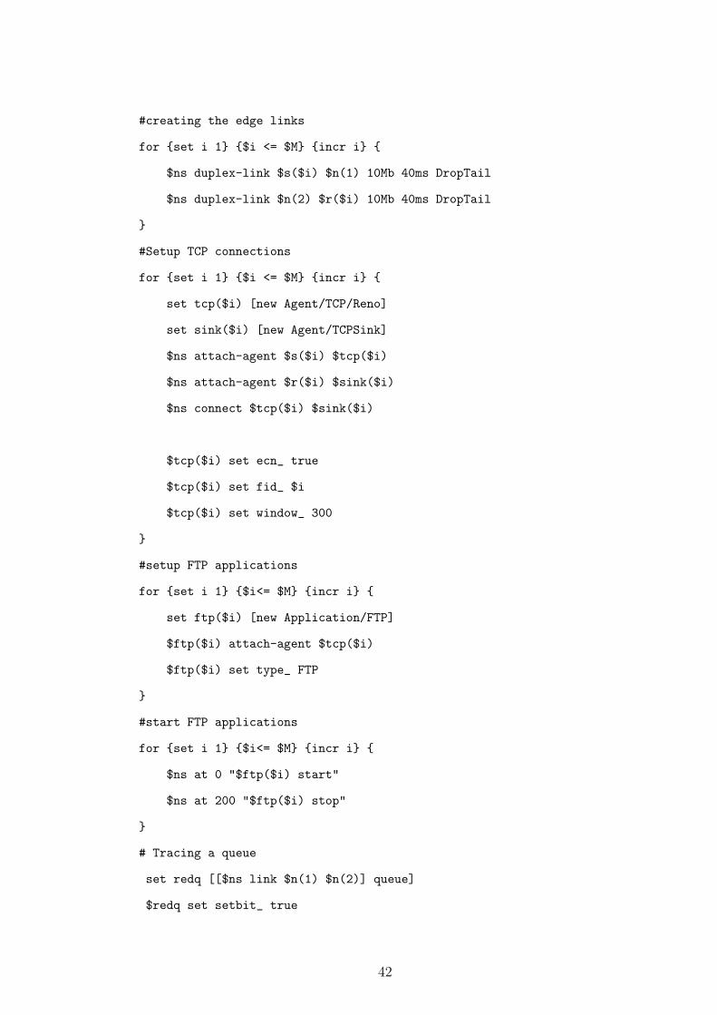
#creating the edge links
for {set i 1} {$i <= $M} {incr i} {
$ns duplex-link $s($i) $n(1) 10Mb 40ms DropTail
$ns duplex-link $n(2) $r($i) 10Mb 40ms DropTail
}
#Setup TCP connections
for {set i 1} {$i <= $M} {incr i} {
set tcp($i) [new Agent/TCP/Reno]
set sink($i) [new Agent/TCPSink]
$ns attach-agent $s($i) $tcp($i)
$ns attach-agent $r($i) $sink($i)
$ns connect $tcp($i) $sink($i)
$tcp($i) set ecn_ true
$tcp($i) set fid_ $i
$tcp($i) set window_ 300
}
#setup FTP applications
for {set i 1} {$i<= $M} {incr i} {
set ftp($i) [new Application/FTP]
$ftp($i) attach-agent $tcp($i)
$ftp($i) set type_ FTP
}
#start FTP applications
for {set i 1} {$i<= $M} {incr i} {
$ns at 0 "$ftp($i) start"
$ns at 200 "$ftp($i) stop"
}
# Tracing a queue
set redq [[$ns link $n(1) $n(2)] queue]
$redq set setbit_ true
42

$redq set limit_ 300
$redq set mean_pktsize_ 1000
$redq set qref_ 150
$redq set w_ 4
$redq set a_ 0.000045351
$redq set b_ 0.000042821
set tchan_ [open PI_new_09_09.txt w]
$redq trace curq_ $redq
attach $tchan_
# Define ’finish’ procedure (include post-simulation processes)
proc finish {} {
global tchan_
set awkCode {
{
if ($1 == "Q" && NF>2) {
print $2, $3 >> "temp.q";
set end $2
}
else if ($1 == "a" && NF>2)
print $2, $3 >> "temp.a";
}
}
set f [open temp.queue w]
puts $f "TitleText: PI_new_09_09"
puts $f "Device: Postscript"
if { [info exists tchan_] } {
close $tchan_
}
43

exec rm -f temp.q temp.a
exec touch temp.a temp.q
exec awk $awkCode PI_new_09_09.txt
puts $f \"queue
exec cat temp.q >@ $f
#puts $f \n\"ave_queue
#exec cat temp.a >@ $f
close $f
exec xgraph -bb -tk -x time -y queue temp.queue &
exit 0
}
#Call the finish procedure after 200 seconds of simulation time
$ns at 201 "finish"
#Run the simulation
$ns run
44

Bibliography
[1] K. J. Astrom, T. Hagglund, PID Controllers: Theory, Design, and Tuning,
2nd Ed., Instrument Society of America, Research Triangle Park, NC, 1995.
[2] S. Athuraliya, S. H. Low, V. H. Li, Q. Yin, “REM: Active Queue Manage-
ment,” IEEE Network, vol. 15, no. 3, May-June 2001, pp. 48-53.
[3] M. di Bernardo, F. Garofalo, and S. Manfredi, “Performance of Robust AQM
controllers in multibottleneck scenarios,” Proc. of the 44th IEEE Conference
on Decision and Control, and the European Control Conference 2005 Seville,
Spain, December 2005, pp. 6756–6761.
[4] S. Floyd, V. Jacobson, “Random early detection gateways for congestion
avoidance,” IEEE/ACM Transactions on Networking, vol. 1, no. 4, Aug.
1993, pp. 397-413.
[5] S. Floyd, K. Fall, “Promoting the use of end-to-end congestion control in the
Internet,” IEEE/ACM Transactions on Networking, vol. 7 (1999), pp. 458–
472.
[6] G. C. Goodwin, S. F. Graebe, and, M. E. Salgado Control System Design,
Prentice Hall, 2001.
[7] A. N. Gundes, H. Ozbay, A. B. Ozguler, “PID Controller Synthesis for
a Class of Unstable MIMO plants with I/O Delays,” Automatica, vol. 43
(2007), pp. 135–142.
45

[8] C. Hollot, V. Misra, D. Towsley, W. Gong, “On designing improved con-
trollers for AQM routers supporting TCP flows,” in IEEE INFOCOM,
Alaska, April 2001, pp. 1726-1734.
[9] C. Hollot, V. Misra, D. Towsley, W. Gong, “Analysis and design of con-
trollers for AQM routers supporting TCP flows,” IEEE Transactions on
Automatic Control, vol. 47, no. 6, June 2002, pp. 945-959.
[10] R. Isermann, Digital Control Systems Volume 1: Fundamentals, Determin-
istic Control, 2nd revised Ed., Springer-Verlag, 1989.
[11] F. Kelly, “Mathematical modeling of the Internet,” Mathematics Unlimited-
2001 and Beyond, B. Engquist and W. Schmidt Eds., Berlin, Germany,
Springer-Verlag, 2001.
[12] S. Kunniyur, R. Srikant, “Analysis and design of an adaptive virtual queue
(AVQ) algorithm for active queue management,” in Proc. ACM SIGCOMM,
San Diego, CA, Aug. 2001, pp. 123-134.
[13] Y. Lee, J. Lee, S. Park, “PID controller tuning for integrating and unstable
processes with time delay,” Chemical Engineering Science , vol. 55, 2000,
pp. 3481-3493.
[14] V. Misra, W. Gong, D. Towsley, “Fluid-based analysis of a network of AQM
routers supporting TCP flows with an application to RED,” in Proc. ACM
SIGCOMM, Stockholm, Sweeden, Sep. 2000, pp. 151-160.
[15] ns-2 Network Simulator, version: 2.27. [Online]. Available:
http://www.isi.edu/nsnam/ns/.
[16] K. Ogata, Modern Control Engineering, 3rd Ed., Prentice Hall, 1997.
[17] H. Ozbay, A. N. Gundes, “Resilient PI and PD Controllers for a Class of
Unstable MIMO plants with I/O Delays,” in CDROM Proceedings of 6th
IFAC Workshop on Time Delay Systems, L’Aquila, Italy, July 2006.
46

[18] P-F. Quet, H. Ozbay, “On the Design of AQM Supporting TCP Flows Using
Robust Control Theory ,” IEEE Transactions on Automatic Control, vol.
49 (2004), no. 6, pp. 1031-1036.
[19] E-C. Park, H. Lim, K-J. Park, C-H. Choi, “Analysis and design of the virtual
rate control algorithm for stabilizing queues in TCP networks,” Computer
Networks, vol. 44 (2004), pp. 17-41.
[20] E. Poulin, A. Pomerlau, “PI Settings for Integrating Processes Based on
Ultimate Cycle Information” IEEE Transactions on Control Systems Tech-
nology, vol. 7, 1999, pp. 509-511.
[21] K. Ramakrishnan, S.Floyd, “A Proposal to add Explicit Congestion Notifi-
cation (ECN) to IP,” RFC 2481, January 1999.
[22] S. Ryu, C. Rump, C. Qiao, “A predictive and robust active queue manage-
ment for Internet congestion control,”in Proc. of the 8th IEEE Symposium
on Computers and Communications, Kemer, Antalya, Turkey, June-July
2003, pp. 991–998.
[23] S. Ryu, C. Rump, C. Qiao, “Advances in Internet Congestion Control,”in
IEEE Communications Surveys and Tutorials, vol. 5, no. 1, Third Quarter
2003, pp. 28-38.
[24] G.J. Silva, A. Datta, S. P. Bhattacharyya, PID Controllers for Time-Delay
Systems, Birkhauser, Boston, 2005.
[25] P. Yan, Y. Gao, H. Ozbay, “A Variable Structure Control Approach to
Active Queue Management for TCP with ECN,” IEEE Transactions on
Control Systems Technology, vol. 13, no. 2, March 2005, pp. 203-215.
[26] P. Yan and H. Ozbay, “Robust Controller Design for AQM and H∞ Per-
formance Analysis,” in Advances in Communication Control Networks, S.
Tarbouriech, C. Abdallah, J. Chiasson Eds., Springer-Verlag LNCIS, Vol.
308, 2004, pp. 49-64.
47


![Pi Pid Controller[eBook.veyq.Ir]](https://img.dokumen.tips/doc/110x75/577cd44b1a28ab9e789821ba/pi-pid-controllerebookveyqir.jpg)