A new class of algorithms for classical plasticity extended to

Computational Mechamcs (1993) 11,253 278 Computational Mechanics @ Springer-Verlag 1993

A new class of algorithms for classical plasticity extended to finite strains. Application to geomaterials*

J. C. Simo and G. Meschke Division of Applied Mechanics, Department of Mechanical Engineering, Stanford University, Stanford, CA 94304, USA

Abstract. A recently proposed methodology for computational plasticity at finite strains is re-examined within the context of geomechanical applications and cast in the general format of multi-surface plasticity. This approach provides an extension to finite strains of any infinitesimal model of classical plasticity that retains both the form of the yield criterion and the hyperelastic character of the stress strain relations. Remarkably, the actual algorithmic implementation reduces to a reformulation of the standard return maps in principal axis with algorithmic elastoplastic moduli identical to those of the infinitesimal theory. New results in the area of geomechanics include a fully implicit return map for the modified Cam-Clay model, extended here to the finite deformation regime, and a new semi-explicit scheme that restores symmetry of the algorithmic moduli while retaining the unconditional stability property. In addition, a new phenomenological plasticity model for soils is presented which includes a number of widely used models as special cases. The general applicability of the proposed methodology is illustrated in several geomechanical examples that exhibit localization and finite deformations.

1 Introduction

Currently, there is a well-developed framework for the algorithmic treatment of classical infinitesimal plasticity. Two key ingredients are (i) The so-called return mapping algorithms which, for associative plasticity reduce the incremental integration of the plastic flow evolution to a convex minimization problem, and (ii) The so-called algorithmic elastoplastic moduli, obtained by consistent linearization of the return mapping algorithm. Return mapping algorithms were simultaneously introduced by Wilkins (1964) and Maenchen and Shack (1964) in the context of J/-flow theory, and subsequently generalized by a number of authors in a different context; see Simo and Hughes (1990) for a comprehensive review. The key interpretation as a convex optimization problem goes back at least to Moreau (1976). The notion of algorithmic (as opposed to continuum) tangent elastoplastic moduli was first introduced in Simo and Taylor (1984), leading to a significant improvement in performance of iterative solution schemes employing Newton and quasi-Newton methods.

Extensions to the finite strain regime of classical models of plasticity have typically relied in the past on hypoelastic rate formulations of the stress response. Fundamental questions aside, such extensions make the task of generalizing the standard return maps of the infinitesimal theory cumbersome, while rendering practically impossible the derivation ~f the algorithmic moduli. In sharp contrast with this state of affairs, the extension to finite strains of classical infinitesimal plasticity models advocated herein possesses the following properties:

(i) The stress response is hyperelastic and, consistent with a multiplicative decomposition of the deformation gradient, characterized by means of a stored energy involving only the elastic part of the deformation gradient.

(ii) The definition of the elastic domain is identical to that of the infinitesimal theory, with the stresses now interpreted as true stresses acting on the current configuration of the body. We remark that the specification of the elastic domain in terms true stresses necessarily restricts the theory to isotropic yield criteria.

* Partial support provided by the Max Kade Foundation under Grant No. 2-DJA-616 and with Stanford University, and the Naval Civil Engineering Laboratory at Port Huaneme

254 Computational Mechanics 11 (1993)

(iii) The associative form of the flow rule compatible with a multiplicative decomposition of the deformation gradient is uniquely defined by resorting to the principle of maximum plastic work.

From a computational perspective the central issue concerns the numerical integration of the evolution of plastic flow. Remarkably, by applying an exponential approximation to the flow rule in the form recently proposed in Simo (1991), one exactly recovers the standard return mapping algorithms of the infinitesimal theory, now formulated in principal Eulerian axes. Within this approximation, the algorithmic elastoplastic moduli in principal axes coincide with the algorithmic moduli of the infinitesimal model. In summary, the actual implementation in the finite strain regime of a classical model of infinitesimal plasticity involves two steps:

(iv) A trial elastic state computed by an approach identical to that recently described in Simo and Taylor (1991) for finite hyperelasticity formulated in principal stretches.

(v) A corrector step defined by a return mapping identical to that of the infinitesimal theory, now formulated in fixed Eulerian principal axes defined by the trial state.

We remark that the tangent operator (the Hessian) in this formulation is symmetric and possesses a structure identical to that of finite elasticity formulated in principal stresses, with material tangent in principal axis identical to the algorithmic elastoplastic moduli of the infinitesimal theory.

A main goal of this work is to demonstrate the effectiveness and general applicability of the preceding computational framework to the complex models of phenomenological plasticity that arise in geomechanical applications. Two specific applications are considered. In Sect. 4 a formulation and algorithmic treatment of the modified Cam-Clay model of Roscoe and Burland (1968) is presented within the realm of true finite strains. In addition to (necessarily non-symmetric) fully implicit schemes, an alternative class of new semi-implicit return maps is described which restores the symmetry of the algorithmic moduli while retaining the property of unconditional stability. In Sect. 5 we undertake the formulation of a fairly general class of phenomenological models of plasticity which include as special cases widely used models in soil mechanics. Since the algorithmic treatment of this class of models is identical to that of the infinitesimal theory, now formulated in principal stretches, further discussion on computational aspects is omitted. The reader is directed to Simo et al. (1988) for a comprehensive discussion. Section 6 describes a number of representative simulations in geomechanics, exhibiting localization and finite deformations, which demonstrate the effectiveness of the proposed methodology. Conclusions are drawn in Sect. 7.

2 Multiplicative elastoplasticity at finite strains

We give a concise outline of a formulation of plasticity at finite strains in which the elastic domain IE is specified by any classical model of infinitesimal plasticity, with the stress tensor now interpreted as the true (Kirchhoff) stress tensor acting on the current configuration of the body. As in the infinitesimal theory, in the present formulation the associative form of the evolution equations is uniquely defined via the principle of maximum plastic work (Hill 1950). Throughout this presenta- tion attention is restricted to the purely mechanical theory. For a complete thermodynamical treatment we refer to the recent work of Simo and Miehe (1991).

2.I Motivation: The infinitesimal theory

To motivate our subsequent developments we summarize first the key assumptions underlying a classical model of infinitesimal elastoplasticity. In fact, the formulation of finite strain plasticity described below will be constructed by specifying a direct counterpart of these assumptions. In particular, the standard evolution equations describing associative plastic flow can be uniquely extended to finite strains via their equivalent statement in terms of maximum plastic work.

i. Elastic domain. A convex elastic domain IE defined by a m-convex yield functions defined in

J. C. Simo and G. Meschke: A new class of algorithms for classical plasticity 255

stress space and intersecting (possibly) in a non-smooth fashion; i.e.,

IE = {(~, q)~S x lR'~=~:q~u(~, q) < 0, for # = 1, 2,..., m}, (2.1)

where S is the vector space of symmetric rank-two tensors and q is a suitable vector of m~,t > 1 (stress-like) internal variables characterizing the hardening response of the material.

ii. Additive decomposition and free energy. The total infinitesimal strain tensor is decomposed additively into elastic and plastic parts as

~.(X, t) = ~.e(x, t) + gP(X, t). (2.2)

The elastic response of the material is assumed to depend only on the elastic part e~ and is characterized by means of a free energy function ~b(e ~, or). Here a~ is the vector of (strain-like) internal variables conjugate to q; i.e., q:= - c3~.

iii. Associative evolution of plastic flow. Restricted to the purely mechanical theory the dissipation function ~ is the difference between the stress power and the rate of change of the internal energy. The second law then implies

~@ = 'I"~ - - ~(,~e, 0D ) 0. (2.3)

Clearly ~ -= 0 for an elastic material. The simplest model that describes the evolution of the internal variables {Z, ~} corresponds to the assumption of maximum dissipation. According to this postulate, among all possible admissible states ('~, ~)eIE the actual state (~, q)slE is that leading to maximum dissipation for prescribed rates of deformation. Maximum plastic dissipation is the key property of associative plastic flow amenable to a unique and straight-forward generalization to the finite strain regime. As a motivation, we show below how this assumption yields the classical evolution equations describing associative plastic flow.

2.1.1 Constitutive equations. Dissipation inequality. The three assumptions above completely define the evolution equations of classical plasticity, as follows. First, using the chain rule expression (2.3) for the dissipation function becomes

= [~ - c~o~b].~ + ~e~b" E~ - / ;e l + [ _ c~,~b] "d~ > 0. (2.4)

Since Eq. (2.4) is to hold for all admissible processes, a standard argument produces the stress-strain relations and the reduced dissipation inequality:

= ~?~b(~ e, ~) and ~ = t" [/~ - U] + q" & > 0, (2.5)

where q = - c3a@(~ e, 0 0. Second, with this expression in hand the assumption of maximum plastic dissipation translates into the inequality:

[ ~ - ~ ] . [ ~ - U ] + [ q - ~ ] . & > 0 , V(~,q)~IE. (2.6)

Consequently, if the elastic domain IE is defined by the convex set (2.1), a standard result in convex analysis shows that inequality (2.6) holds if and only if the following conditions hold:

U = k - ~ 7,~?,qSU(~,q), &= ~ 7u~q(aU(~,q), 7 ,>0 , q~u(T,q)<0, ~ 7,qSU(~, q) -- 0, (2.7) ,u=l #=1 #=1

which furnish the standard local form of the evolution equations for associative plasticity. We remark that the maximum dissipation inequality (2.6) leading to (2.7) plays a central role both in the mathematical theory and in the numerical analysis of classical plasticity (see e.g., Simo (1991a) and references therein).

2.2 The nonlinear theory. Basic assumptions

In our formulation of classical models of infinitesimal elastoplasticity in finite strain regime we retain the form of elastic domain IE in the infinitesimal theory with v now interpreted as the

256 Computational Mechamcs 11 (1993)

Kirchhoffstress tensor in the current configuration. This key design condition defines the structure of the nonlinear theory as follows.

i. Elastic domain. For simplicity, attention is restricted in this section to a single scalar hardening variable; thus

IE:= {(~, q)eS x IR: q~"(~, q) __< 0 for/~ = 1,2,...,m}. (2.8)

We remark that the principle of objectivity restricts the possible forms of q5 in Eq. (2.8) to isotropic functions. Consequently, a classical formulation of the yield criterion in terms of true stresses necessarily imposes the restriction to isotropy of the resulting theory.

ii. Multiplicative decomposition and free energy. The generalization to finite strains of the additive decomposition used in the infinitesimal theory is motivated by the structure of the single crystal models of metal plasticity, and takes the form of the local multiplicative decomposition

F(X, t) = Fe(x, t)FP(X, t) (2.9)

where F(X, t):= Do(X, t) denotes the deformation gradient of the motion q~(., t) at X ~ . From a phenomenological point of view F p is an internal variable related to the amount of plastic flow while F e- 1 defines the local, stress-free, unloaded configuration. Consistent with the restriction to isotropy it is further assumed that ~ is independent of the orientation of the intermediate configuration. Frame invariance then implies the functional form

0=tp(b~,~), where b~:=FeF ~r. (2.10)

The measure of elastic deformation b e defined above is the elastic left Cauchy-Green tensor.

iii. Associative evolution of plastic flow. The local dissipation function ~ per unit of reference volume associated with a material point Xe:~ is defined as the difference between the local stress power and the local rate of change of the free energy; i.e.,

~ : = x ' d - ~(be, c~) > 0. (2.11)

Here d = sym [1] denotes the rate of deformation tensor and 1:= ~'F- 1 is the spatial velocity gradient. As in the infinitesimal theory, the simplest model describing the evolution of plastic flow is obtained by postulating maximum dissipation of the flow.

Following an argument entirely analogous to that used for the infinitesimal theory, we show below that the preceding assumptions uniquely define a model of associative plasticity at finite strains.

2.3 Constitutive equations. Dissipation inequality

Our first objective is to obtain an explicit expression for the dissipation. The rate of change ~ is computed by exploiting the relation

b e = FCP-IF r with CP:= FprF p, (2.12)

which follows from the multiplicative decomposition (2.9), and identifies C p as the plastic right Cauchy-Green tensor. Time differentiation of this expression yields the identity

[je:lbe+belr+~.~vbe with ~q~b~:=F~[Cp-1]F r, (2.13) d t

where ~vb e is referred to as the Lie derivative of b e. Time differentiation of the free energy function and use of the relation (2.13)1 yields the result

d/,4 ~-~ = aboO'l~ e + cg,0~ = [28boObe] �9 El + �89176 e- 1] + 8 ~ . dt

(2.14)

Since b e commutes with c?b~ p as a result of the restriction to isotropy, combining Eq. (2.14) and


Eq. (2.11) yields the following local form of the dissipation inequality:

= [~ - 2C3be0be]-d + [2~bo~tbe].[-�89 ] + [-- 0a~]~ => 0, (2.15)

which furnishes the finite strain counterpart of (2.4). Since (2.15) must hold for all admissible processes, the same standard argument used in the infinitesimal theory now gives the following constitutive equations and the reduced form of the dissipation inequality

~ = 2c3b~0b e, ~ =,c.[ 15(~v b e ) b e - 1] + qo~ > 0,~___ (2.16)

with q:= -~?=~p. These relations are the finite strain counterpart of relations (2.5).

2.3.1 Associative evolution equations. Maximum dissipation. According to the postulate of maximum dissipation the actual state (~, q)elE in the plastically deformed body at a given (fixed) configuration, with prescribed intermediate configuration and prescribed rates {&t'~,b e, 0i}, renders a maximum of the dissipation function 9. Equivalently, the following inequality holds:

Ix - ~3.[ - l(~q~~ 13 + [q - ~]0i > 0, (~, ~/)6IE. (2.17)

This result is the counterpart of inequality (2.6) in the finite strain regime. As in the infinitesimal theory, inequality (2.17) holds if and only if the coefficients {--l(~.~vbe)be-l,~ } lie in the cone normal to c?IE at the point (x, q). In particular, if ~?IE is defined by Eq. (2.8), the evolution equations read

# = i

,u=l

7u0~qSr z, q)] be

7u~qqSU( ~, q)]

7 ,>0 , q~U(~,q)__<0 and ~ 7u~bU(~,q)=0. (2.18) ,u=l

Despite its unconventional appearance (compare with the corresponding expression (2.7) in the infinitesimal theory) the flow rule (2.18) possesses a number of interesting properties. In particular, it gives the correct evolution of plastic volume changes as the following observations show.

(i) The total and elastic volume changes are given by J := det IF] > 0 and je: = (det [b e])1/2 > 0, respectively.

(ii) Let JP:= det [FP]. Setting e"'= log [JP] the rate of plastic volume change predicted by the /)"

flow rule (2.18)1 is given by the evolution equation

i p= ~ 7, tr[~,b"] , (2.19) #=1

which implies exact conservation of plastic volume for pressure insensitive yield conditions; i.e. if tr[0~4~"] = 0.

The proof of the result in Eq. (2.19) follows easily from Eq. (2.13) along with Eq. (2.18)1. The foregoing theory will be applied to a number of classical models in soil mechanics in the following sections.

2.3.2 General non-associative evolution equations. Expression (2.18) provides a crucial insight in the extension to finite strains of non-associative models of infinitesimal plasticity. For instance, for single-surface plasticity (i.e.,/t = 1) the non-associative flow rule takes the form

k e = ~ - - 7(~9('~, q), 0i = 70qg(~, q), (2.20)

where g:S x IR ~ IR is the plastic flow potential; in general g # q5. The extension of a model of this type to the finite strain regime then takes the form

1 e - - ~ ' v b = [7~?~g(~, q)]b e, ~ = 7~qg(~, q), (2.21)

where g(~, q) has identical form as in the infinitesimal theory.

258 Computa t iona l Mechamcs 11 (1993)

3 Exponential return mapping algorithms

Following Simo (199 lb) we consider an algorithmic approximation consistent with the associative flow rule derived above which is exact for incrementally elastic processes, independent of the specific form adopted for the stored energy function and exact plastic volume preserving for pressure insensitive plasticity models. Remarkably, the implementation of this algorithm takes a form essentially identical to the standard return maps of the infinitesimal theory.

3.1 The local problem of evolution. The algorithmic flow rule

Consider a typical time sub-interval [t,, t,+ 1], an arbitrary material point X e ~ and assume that the deformation gradient F, along with {b e, c%} ES+ x R+ which define the constitutive response of the material, are prescribed initial data at XsN. The objective is to construct an algorithmic approximation to the plastic flow evolution equations for incremental displacement field u t prescribed on tp,(~) x It., t,+ 1], where %(-) is a given configuration at time t, defined on ~. Denoting by ft(x,):= I + Vut(x,) the relative deformation gradient at x, = %(X), the local evolution of plastic flow is governed by the first order constrained system

" e _ [ l t b t + e r __ 2 b t - b t It ] bt

m

7u >0, 0 ( t, qt) < 0 and ~ 7u4 ( t, qt) O, (3.22)

where i, = ~,ff 1 is the spatial velocity gradient. The solution of (3.22) defines {b7, c~t} at the point X within the interval of time [t,, t, + 13 for configuration prescribed by the relation tPt = tp, + uto ~p,.

The key idea in the design of an integration algorithm for Eq. (3.22) is to recast this system as a standard problem of evolution, of the form j? = H(y, t)y, and then apply the exponential approximation y, = exp [AtH(yt, t)]yr This idea is carried out in two steps:

Step 1. Recast Eq. (3.22) in the form of a nonlinear problem of evolution of the form j~ = H(y, t)y. In the present context this is accomplished by pull-back of Eq. (3.22) to the fixed initial configuration tp,(N), as follows. Define the tensor fields

b ; * : = f t l b f f / r , ct:=ftrft and n~:=fr~(~u('c,,qt)f,. (3.23)

In geometric terms " n t, # = 1, 2 , . . , m are interpreted as the pull-back of the normal d~q~U to the configuration (p,(N), with the tensor c t = f f f t viewed as a Riemannian metric on ~p,(N). A straightforward manipulation shows that the system (3.22)1 is equivalent to

~ge* 2 -1 ~ e* (3.24) =- -- b t , with h~*lt=t,, be ~ t t =1 ~/uct nt = n'

which is now written in standard form.

Step 2. Using an exponential approximation to Eq. (3.24) within the interval It,, t ] c [t,, t,+ 1]

I ~ ln~l be' where ATu > 0 is a Lagrange yields the first order accurate formula b~* ~ exp - 2 AT.e t- = i z = l

multiplier to be determined by enforcing consistency as described below. Using Eq. (3.23)1 this relation becomes

b:=(f'explh2 c n lf l)b: tr l where b:tr=fb:f 325,


Fixed Reference Configuration

Fn @ b~ctn

"<, Fn+l ~ tr

b n + l o~ n

Fixed Intermediate Configuration Updated Current Configuration

Fig 3.1. Interpretation of the trial state: The (local) reference and intermediate configurations remain fixed, while the current configuration is updated for prescribed relative deformation gradient

where the symbol ~ has been replaced by the equal sign. The algorithmic approximation is completed by exploiting the well-known property F exp[A]F-1 = exp[FAF-1] , which yields

b t = e x p [ - 2 .=*~ ATu~qSU(rt, qt)]bt tr

at = ~. + ~ ATu0q~u(~t, qt) # = 1

AT,.>0, q~'%,q3 <0, ~ A , ".c = ~,~b ( t, q0 = 0, (3.26) # = 1

where (% qt) are defined by the elastic stress-strain relations evaluated at (bt, at). A standard argument using a Taylor series expansion confirms that the product formula algorithm (3.26) is first order accurate. Unconditional stability follows from the properties of the backward Euler scheme and the exponential map. A geometric illustration of Eq. (3.26) is given in Fig. 3.1.

The derivation of the algorithmic flow rule (3.26) is identical to the algorithmic treatment in Simo (1988), with the backward-Euler scheme replaced here by an exponential approximation. Although both algorithms possess identical accuracy properties, the backward Euler method does not inherit the following conservation properties which are identically satisfied by Eq. (3.26).

(i) Preservation of the constraint det[b[] > 0; a property which follows from the identity det [exp [A] ] = exp [tr [A] ].

(ii) Exact conservation of the plastic volume. For pressure insensitive yield criteria the plastic volume preserving property of the exact flow rule is preserved by the algorithmic approximation, since Eqs. (3.26) implies tr [~?,q~"(~t, q,)] - 0,~JtP = JP ,.

A modification of the backward Euler method which does inherit property (ii) above is given in Simo and Miehe (1991). We remark that both the backward Euler and the exponential approxima- tions become exact for incrementally elastic steps since ATu = 0.

3.2 Spectral decomposition: Formulation in principal axes

By isotropy the principal directions {nlA)}A = 1,2,3 of the Kirchhoff stress tensor ~t coincide with the principal directions of the elastic left Cauchy-Green tensor b~. Let {O-A} and {2A 2 } denote the respective set of principal values. The key to the implementation of the algorithm lies in the following observations:

tr(A) and e t r (i) Let n t '~A > 0 denote the principal directions and the square root of the associated principal values of b~ tr, respectively. Then, from (3.26)~ one immediately concludes that the final principal directions coincide with the principal directions; i.e., n~ A) = nlr(A) for A = 1, 2, 3.

260 Computational Mechanics l 1 (1993)

�9 a n d etA . = log denote the logarithmic stretches. Setting ~b(b ~, ~) = (ii) Let I~tA . = log [),ta ] etr. t-"tAI- ]etrq.j

q~(e], ~), the constitutive equations become

e (3 1if(8;, ~t) ' (3.27) f f A = ~ . e . 4 ~ ( e A ' O~t)' qt = - -

which possess a functional form identical to that of the infinitesimal theory. (iii) Set ~b"(,, q) - q~U(al, 0"2, 0"3, q)- Then the algorithmic flow rule collapses to

,e etr ~ A~#~aA ~#(O.t, qt ) ~tA ~ ~'tA - -

#=1

#=1

aTu>0, 6~'(at, qt)<O, ~ aT,6~'(o',,qt)=0, (3.28) / t = l

which along with Eq. (3.27) define a return mapping algorithm at fixed principal axis (defined by the trial state) identical to that of the infinitesimal theory.

The advantage of the preceding scheme is clear: It allows the extension to the finite strain regime of the classical return mapping algorithms of the infinitesimal theory without modification but with the following additional simplification. The return map is now formulated in the principal (Eulerian) axis defined by the trial state, which can be computed in closed form directly from b~ t~, as explained next.

3.3 Closed-form implementation

The step-by-step procedure outlined below summarizes the actual implementation of the updating scheme defined by preceding algorithm within the interval [t,, t,+ 1]. In a finite element context, this update procedure takes place at each quadrature point of a typical element.

Step 1. Trial state. Given {b~,c~,} (at a specific quadrature point x,~q~,(~)) compute the trial elastic left Cauchy-Green tensor and the relative deformation gradient f, + 1 for prescribed deformation u, + 1 : q~,(~) ~ jR3 as

f ,+ l (x , ) := I+ Vu,+l(x,), b ~t~ =f ,+ bef T (3.29) n + l 1 n n + l " ~2 etr Step 2. Spectral decomposition of~ b eta.+1. Compute the principal stretches t , + 1 A } by solving the

cubic characteristic equation in closed form via Cardano's formulae. Compute the principal directions ,fn tr(A)/, via the closed form formula t. . + l J

[- betr (,~etr ~21 7[ - h etr (~L etr "12"1- -] Htr(A) (~ ntr(A) = | - n + 1 ~ '.--n + 1 B ~ | [ --n+ 1 ~ V*n + I_C.' - | (3.30)

n + l ' ~ n + l |r "12__(~etr ~2]|ggetr "~2 (~etr ~ 2 | ' t_,. n + l B / p ' ~ n + l A ? - I I - \ "~n+IC] - - ~ n + l A ! -J

for A = 1, 2, 3, with B = 1 + mod(3, A) and C = 1 + mod(3, B).

Step 3. Return mapping in principal (elastic trial state) axes. Compute the logarithmic stretches and the principal trial stresses:

etr = [-lo_Z~etr ~Letr etr T ~ L g~ n + l l ) , l o g ( n+12),log()~n+13)] o'tr (~ *l~t(getr ~n), tr = - - ~ I~/(Ee tr ~n)" (3.31) qn+l ~t't" ~ n + l n + l ~ "r', n + l ~

Evaluate q~t~+ 1 = q~(tr~§ ~,q~+ ~). If q~tr+ 1 > 0 perform the return mapping algorithm (see remarks below) to compute {e~ + t, ~, + 1 }. Compute the Kirchhoff stress tensor via the explicit formula

3 ~tr(A) ~ B, tr(A) (3.32)

~ n + l = E f f n + l A S | A = I

e where 0-,+ 1A = ~,~tp(e + 1, ~,+ 1) are the principal Kirchhoff stresses.


/

o ,/' \ , \ Ck=O

................... . 1 / r

Fig. 3.2. Geometric interpretation of the return mapping algorithm for multlsurface plasticity in principal stress space for two possible trial elastic states

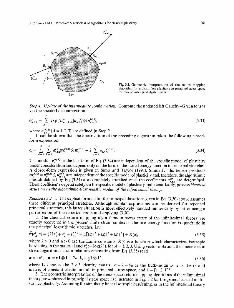
Step 4. Update of the intermediate configuration. Compute the updated left Cauchy-Green tensor via the spectral decomposition

3 = j•tr(A) ~ ntr(A) (3.33) b~,+2 ~ exp[2~+IA- , + l ~ - - , + l ,

A = I

w h e r e n tr{A) (A = 1, 2, 3) are defined in Step 2. n + l It can be shown that the linearization of the preceding algorithm takes the following closed-

form expression: 3 3 3

Ct= Z Z he" mtr(A)(~mttr(B)- t - 2 ~, ' - otr(A) (3.34) UtA~.t ~ tAB '" t A = I B=I A = I

mA) in the last term of Eq. (3.34) are independent of the specific model of plasticity The moduli c~ under consideration and depend only on the form of the stored energy function in principal stretches. A closed-form expression is given in Simo and Taylor (1991). Similarly, the tensor products mma) = ,tr(A) ~ ,tr(A) are independent of the specific model of plasticity and, therefore, the algorithmic t "'n + 1 "r "'n + 1 moduli defined by Eq. (3.34) are completely specified once the coefficients a~]~ are determined. These coefficients depend solely on the specific model of plasticity and, remarkably, possess identical structure as the algorithmic elastoplastic moduli of the infinitesimal theory.

Remarks 3.1 1. The explicit formula for the principal directions given in Eq. (3.30) above assumes three different principal stretches. Although similar expressions can be derived for repeated principal stretches, this latter situation is most effectively handled numerically by introducing a perturbation of the repeated roots and applying (3.30).

2. The classical return mapping algorithms in stress space of the infinitesimal theory are exactly recovered in the present finite strain context if the free energy function is quadratic in the principal logarithmic stretches; i.e.:

~(,~A,~) 1 e = + + ;12 + + (3.35)

where 2 > 0 and/~ > 0 are the Lam6 constants,/((.) is a function which characterizes isotropic hardening in the material and Ca:= log(2]), for A = 1, 2, 3. Using vector notation, the linear elastic stress-logarithmic strain relations emanating from Eq. (3.35) read

o'=ag e, a : = t c l | + 2 / / [ I 3 - � 8 9 1 7 4 (3.36)

where 13 denotes the 3 x 3 identity matrix, ~c:= 2 +-~// is the bulk-modulus, a is the (3 x 3) matrix of constant elastic moduli in principal stress space, and 1 = [1 1 1] r.

3. The geometric interpretation of the stress-space return mapping algorithms of the infinitesimal theory, now phrased in principal stress space, is illustrated in Fig. 3.2 for the general case of multisurface plasticity. Assuming for simplicity linear isotropic hardening, as in the infinitesimal theory


one can show that (Simo 1991b)

[fl o.+13.a-1 _ t r -- [o,+ 1 - a . + l ] + [ ~ / - q . + ~ ] H - l [ q . - q . + l ] < 0 V(II, q)~IE. (3.37)

Standard results in convex analysis yield the following interpretation of inequality (3.37): The final state ( ~, + 1, q, + 1)~IE in principal stress space is the closest point projection of the trial state (at, r+ 1, q,) onto the elastic domain in the metric defined by the inverse moduli (a -a, H-1). This result reduces the algorithmic problem in principal Kirchhoff stress space to the standard problem in convex optimization: Find the distance of a point (the trial state) to a convex set (the elastic domain) in a given metric (the inverse elastic moduli). The standard algorithm for this problem is a variant of the gradient-projection method proposed in Simo et al. (1988).

Form a practical standpoint, the preceding developments translate into the following prescrip- tion for the implementation in the finite strain regime of any infinitesimal model of classical plasticity.

(i) Express the model in principal axes. Note that the classical linear infinitesimal elastic stress- strain relations translate into a linear relation between principal Kirchhoff stresses and principal logarithmic strains.

(ii) Construct the algorithmic counterpart of the model (in principal axes) by applying the standard return mapping algorithms, along with the algorithmic elastoplastic moduli a ep (in principal axes).

This defines Step 3 in the step-by-step outline of the algorithm given above. The other steps in this algorithm are independent of the specific elastoplastic constitutive model and remain, therefore, unchanged.

4 Finite deformation Cam-Clay

The methodology presented in the preceding sections is exploited here in the extension to the finite strain regime of a classical model of soil mechanics: the modified Cam-Clay model of Roscoe and Burland (1968). This model remains one of the most widely used plasticity models in geo- technical applications due to its capability of predicting (at least qualitatively) the most relevant characteristics of the mechanical behavior of cohesive soils; see e.g. Wood (1990) for an elaborated discussion. The modified Cam-Clay Model is characterized by ellipsoidal-shaped yield surfaces in the stress space, an isotropic hardening and softening mechanism and by a nonlinear elastic constitutive law.

Algorithms for the Cam-Clay model restricted to the infinitesimal theory have been considered by Ortiz and Simo (1986), within the framework of their (explicit) cutting plane algorithms, and Borja and Lee (1990) using the standard return maps of classical plasticity in conjunction with an explicit treatment of the nonlinear elastic law, among others. An implicit treatment of the elastic law is proposed in Borja (1991), outside the scope of the standard return maps, with the evolution of the void ratio treated explicitly and non-symmetric algorithmic moduli. Here, in addition to a formulation of the Cam-Clay model in the regime of finite strains, we address a number of novel algorithmic aspects; in particular:

(i) An implicit algorithmic treatment of the nonlinear elastic constitutive law along with an implicit integration of the flow rule and the hardening laws which conforms to the now standard return mapping algorithm of classical plasticity.

(ii) An alternative semi-explicit integration scheme which retains the implicit character of the return mapping algorithm while adopting an explicit integration of the hardening law. The key advantage of this approach is the restored symmetry of the algorithmic tangent matrix, achieved without loss of unconditional stability.

4.1 Nonlinear elasticity

A characteristic feature of Cam-Clay is the nonlinear elastic relationship between the (Kirchhoff) pressure p and the elastic volumetric strain e e. Here we incorporate this effect via a stored energy


function of the form:

1 3 co(e e, e~):= U(e e) + CYO(eA) = U(e e) + 2G-iz A=~I (eeA)2' A = 1,2,3, (4.1)

where e~, e 2, e 3 are the principal deviatoric elastic (logarithmic) strains. In what follows, it is more convenient to use the dual form of Eq. (4.1) obtained via the Legendre transformation as

3 2 A = 1,2,3, (4.2) Z sA, Z(P, SA):= )?(p) + 2(SA) = ~(p) + 4 A =1

where st, s2, ss are the principal deviatoric (Kirchhoff) stresses and G denotes the (constant) shear modulus. The specific form of)~(p) is derived below from the following rate form of the volumetric stress-strain specific to the Cam-Clay model

~e:= )7,,(p)/~ = f~e(p)/v(p). (4.3)

Here v is the specific volume in loading processes while v ~ is the specific volume in unloading/ reloading processes (Roscoe and Burland 1968). These specific volumes are related to the pressure via the relations

v(p) :=N-21og(-p) , ve(p):=N--Klog(--p) for p N - 1 , (4.4a)

where N is a material parameter defined as the specific volume at unit compressive pressure, 2 denotes the consolidation index and ~c is the swelling/recompression index. (Note that compression is associated with a negative sign). Since positive values ofp may occur in practical boundary value problems, the following linear extension of Eq. (4.4a) is considered in what follows:

v(p):=N+2(l+p) , ve(p):=N+K(l+p) for p > - l . (4.4b)

Substituting Eq. (4.4) into Eq. (4.3) gives

K

- p ( N _ 2 1 o g ( _ p ) ) ~ if p_-<- l , V

K N + 2(1 + p ) / ~ otherwise.

(4.5)

1 The constitutive equation for the elastic deviatoric (logarithmic) shear strains is e A = ~ SA, while the volumetric part is computed by integrating Eq. (4.5) in time to obtain

61~ 1 - r / l~ ~-r-rl ] ; 7-7S. if p < - l , ~e = )~,(p) = (4.6)

( ~/ p ) otherwise, 6log l + l + t l

2 where 6 = K and q = --. Finally, the inverse relation gives the pressure as the gradient of the volu-

2 N metric part of the stored energy function via the following explicit expression:

- -expU!- - - (~-~)exp( -~) lLr / if e:<61og(1-~q) ,

p = U'(e~) = 1 + t 1V ['e~'~ 7 (4.7) - ~ - L exp ~ ~ ) -- 1 J otherwise.

264

3 ~ z Critical State Line

subcritical

p -

Computational Mechanics 11 (19931

Fig. 4.1. Cam-clay: Meridional sections and critical state hne

4.2 Structure of the model

The yield function may be formulated in the following (generalized) convex format:

+ M 2 - +3 2 f(I1,J2,q(oO):=~fJ2-~-(I 1 ~ q ) M 2, /~ q ---- 0, (4.8) ~ g

where T 1 = 11 - 3t, t denotes the hydrostatic strength of the soil, M is the slope of the critical state line in the ~//~z - p-plane and the hardening parameter q(~) represents the consolidation pressure (Fig. 4.1).

The evolution of the plastic strains and of the hardening variable ~ is governed by an associative flow rule

Of ~P= Of e~=?~s~'~, v Y~pp, A=1,2 ,3 , (4.9)

along with the hardening rule

v(/3) q, d ~ ~p___ Of /3:= p -- t. (4.10) (l=-H(p,q)d~, H:= 2-- ~ Y~pp'

of of Note, that the hardening law is nonassoeiative in the sense that 0i = 7 ~pp ~ Y ~qq.

Remarks 4.1 1. The yield function (4.8) and the hardening law (4.10) differ from the original formulation of the modified Cam-Clay model (see Burland and Roscoe 1968) in that the soil cohesion represented by t is taken into account. Consideration of t may also be useful in the simulation of hydrostatically prestressed conditions arising, for example, in standard triaxial tests. If t is to be considered, the elastic constitutive laws (4.6), (4.7) need to be modified by substituting p and e~ by/~: = p - t and g~ = ~ + s_~, respectively, where e~, t is obtained from Eq. (4.6) as s~(p = - t).

2. Since c) changes sign with --,~ stress states on the subcritical (supercritical) side of the critical 0p

state line (Fig. 4.1) are associated with hardening (softening).

4.3 Fully implicit integration algorithm

The numerical integration scheme for the model falls within the general scheme described in Sect. 2 and will not be further discussed here. The only observation to be made concerns the specific (non-associative) form of the hardening law (4.10). A convenient approach which reduces the

J. C. Simo and G. Meschke: A new class of algori thms for classical plasticity 265

problem to the standard situation discussed in Sect. 2 and involves only replacing ~e_ by ~- adding cq cp

2 terms in the algorithmic tangent, proceeds as follows. We integrate (4.10)~ over a finite time step It,, t, + ~ ] and use the fact that c~ = B~. In the k-th iteration within It,, t, + ~ ], the elastic volumetric strain is given as

B;(k) = /~;,tr 0~(k) ..~ ~n, (4.11)

where B~ 'tr = 1og(je). Hence, the pressure p(e~) may be expressed as a function of the plastic hardening variable c~. Implicit integration of Eq. (4.10)1 yields the following expression for q(k)(ee(k)(c~(k))):

q(k)(~tk))=q, exp p exp e x p ~ - - ) ) ] , (4.12)

where

+ ge = /~e + Be ge.tr = Be,tr _~_ Be a n d p -

V I) v ~ t ' U V V~t ' )~-- tr

The complete algorithm is summarized in Box 4.1. The resulting algorithmic tangent matrix a ep is obtained from the moduli Atj, i , j = 1,..., 4 as

a~a~= ~ A n - - ( n A ' m B ) / ( h / A ~ , ' h , ) , A , B = 1,2,3, r ,s = 1,... ,4, (4.13)

with 3

~An = Aan + AA4 + A4B + A44 -- 2 (AAc + Agc)/3 (4.14a) C = I

and

na = (Aar + A4~)'h~, m a -= ( A r a + Ar4) '~lr . (4.14b)

As a result of the nonassociative hardening law, a ep is nonsymmetric.

Box 4.1. Fully implicit return mapping algorithm for Cam-Clay

1. Initialize: k = O, eP(~ + x = ee., gev,(O) = Bv,e tr ..~ Bey,t, ~ n +~(O) 1 = O~n' In +~(O) 1 = O. 2. Evaluate the pressure, the hardening parameter, the elastic bulk modulus and the hardening

modulus: p~k) U,(ge~k~)

[- // //~e(k) ~ //~e,tr"~ '~ q

q,k)= q. exp L p ~exp ~ ~ ) -- exp ~ - ) ) J,

Klk = l(plk _ t),

_ v ( p - t ) q(k .

3. Evaluate residual and check convergence:

f(k) = f(s~k), p(k), q(k)), sT = [-St , $2 ' $3],

/,(k) ~ -~(k)-{-0~tr )~_~f/(k), hT=[~fs,~fpl"

if f ( k ) < T O L and Ihrl < T O L then EXIT. (Continued)

266 Computat ional Mechanics 11 (1993)

4. Linearize the above equations and compute the algorithmic moduli:

r (k) + A (k)-' i { As \/(k)+ A? ~(k)= 0, \Ap/

!(.~ • 3) 1 + ~ _ _

FA(k) ] - t _ ~s2 t-" ~(4 x 4)~ O2f

Y t?p t?s

Lgs '~qqJ '

? k TsOp + OsDq K(, k--S/

+ \ Op

5. Solve the linearized problem to obtain A7 (k), Ae p'(k) and A~(k):

As (k) = - 2G Ae p(k)

6. Update s, 0~ and compute ~" ~9"

s(k+ 1) = s(k) -I- A s (k), ~(k+ 1) __~ (z(k) _~ h a ( k ) g;,(k + 1) ~-. g;.tr __ g(k+ 1) ~_ (~n"

Set k ~ k + 1 and goto 2.

4.4 Explicit treatment of the hardening law

The issue of a (hardening-induced) nonsymmetric tangent may be entirely by-passed by retaining the implicit form of the return map in the flow while introducing an explicit treatment of the hardening law. Accordingly, integration of the evolution laws (4.9), (4.10) over a finite time-interval It., t.+ 1] is now achieved by means of the formulae

eP A,. + 1 = ep A,. + ~ ~S A (SA,. + 1' Pn + 1, q . ) , A -= 1, 2 , 3

~p (s~,. + 1, P. + 1, ~P s + q.) V,n q- 1 ~ ,n

q"+ l = q" -- TH'(p"' q") ~P n (sa,., P., q,), (4.15)

U where the gradient ~pp. is evaluated at t.. The consistency parameter 7 (k) in the k-th iteration is

obtained from linearization of Eq. (4.15) altogether with

f(k) = jtsa--~ (k)._~. 1' ~'.+n (k) pq. ) = 0, A = 1,2,3, (4.16) - I n + 1

f(k)--h(k)A(k)r(k) ]'! T [~T2f ~?f l (k) (4.17) AT(k)- c3f(k) ~fl ' ='C u~' ~P J "

h(k)rA(k)h Ik) + ~ H, ~p ,

As pointed out above, the resulting tangent matrix a ep has now a symmetric form which is obtained from Eq. (4.13) along with A Ck) in Box 4.1 merely by setting H (k) = 0 and h = h.

a s

J. C. Simo and G. Meschke: A new class of a lgori thms for classical plasticity 267

= 25 30

= 1.33 ~0 - - ~- ~ ' ~ ' t ." ,,_%~ = 2.0 % --4x-- 2 20 ~- r 'At = 0.33 % - - 15 [- .~" - A t = 0 . . 5 % - - ;~ ~ implici[:~: = 1.33 % --m-,- 10 l-J~ im~lici+:A+ = 2.0 ~, --+~-- + I o ,+,+ = + ++ =

0 ~ , I , I , ~ , I , I , 0 c ~ ' ' ~ ' ~ ' ~ ' + ' + '

0 2 4 6 8 10 12 0 2 4 6 8 10 12

a displacement (cm) b displacement (cm)

Fig. 4.2a and 5. Triaxml test: Pressure-displacement curves from the fully-implicit and the semi-explicit a lgori thm for different time steps and different boundary condi t ions (Cam-Clay model): a rigid platens, 5 frictionless platens

�9 ; . . ' ~ ' : . . . . . . : - : i - ' ' "

~ ? , , t . , ' . ; i " : , ' - . , !--,,..,.. i . . . . . . . . . f +-- .' ; - + " , .~&,~,

: ~ ; ' ; ~ " ! i ! 2 . L" ; - ; - ; - . ' - .2 . r - -~ - - ' - . , i ' ~ " , ' + - , f .-..-. ~ ' o - + - ; ~ . . ; . . I " ~ , 4 . �9 ' r - ' ~ . . . . ' - 2 . - ] . . . . Z, . . , . , . . . . . . . - . . r.~...-.z:...~:...~_= ... . .

" ' - . . . . . 1 " - : +. . . . . . . . . J . , , I - -+ i . . . . . . i ' t . . . . . . . a _ . i . . . . . . ~ - . . . . . . . . i . . . . . .

~-. . . . . . ~ , . , . . . . . . . . . . . . . ,. _ . : .L . . . . + ~"]T. 2 . . . . . . , . . . . . . , . . . . . ~ . , , 1 & . . . , , . . - - . . ~ . . . . . . ~ . . . . .

�9 u - . . . . . . . . . . ~ . _ t / _ " ' . ' -~ + - .'.- ,. ~.. .-~.. . .~ ~" . . . . . t . .~ . ,..~ . ; - , . . ~ ~ . - . b - - T - " E . " T . ' . . , , . . ] - f " . . . . . . . ~ . . . . + . , ' . �9 " ' ~ ' " ; " ; " r " " ~ , r . . . . : . , , : . . . . . . . . , . . . . . . . . . . . , : ?, �9 , . , ,

~-~"+"+ ,2 , . . " ; . ' .'.'- . . . . ~. ~;-" " ' + .......

t ' ; " . . , - . , . " - ' " l ~ - - : : ' ' - ~ " ' "

~:~-:~-}~'-~" r.H :-:::.:.: ':","T, - .... L_ :Y~ ."~":".+ ~k " ~ . . . . . . ~.~,ff

VOL. PL. S T

< - 5 9 0 0 E - 0 2

> - 2 9 0 0 E - 0 2

Fig. 4.3. Triaxial test with rigid platens: Dis t r ibut ion of plastic volumetric strains at u = 8.8 cm (Cam-Clay Model)

4.5 Numerical assessment of the algorithms

In this subsection, a comparat ive evaluation of the time-step sensitivity exhibited by the two proposed algori thms (fully implicit and semi-explicit) is presented in the context of axisymmetric analyses of triaxial compression tests�9 Due to axisymmetry, only one quarter of the specimen (diameter d = 21.5 cm, height h - -53 .34cm) is discretized by 120 axisymmetric 4-node elements. Loading is incrementally applied by prescribing a constant vertical top displacement Au.

Simulation (a) assumes rigid loading platens (fixed horizontal boundary conditions), thus inducing a " b a r r e l i n g ' - - t y p e of deformation, as shown in Fig. 4.3. Simulation (b), on the other hand, assumes perfectly frictionless platens leading to a homogeneous stress state. The material parameter used in the analyses belong to normally consolidated Weald Clay, taken from Wood (1990) as: 2 = 0.088, ~c = 0.031, N = 2.097, M = 0.882, G = 3000 kPa, q0 - t = 138 kPa.

Figure 4.2 contains the pressure-displacement curves obtained from the (symmetrized) fully- implicit and the semi-explicit algorithm for different time steps (Au = 0.0133h/2 and Au = 0.0033h/2 for example (a) and Au = 0.02h/2 and Au = 0.005h/2 for example (b)). As expected, considerable influence of the time-step length is observed for the semi-explicit integration scheme as long as the material is hardening. For moderate ly large time steps ( < 1~o), however, the accuracy of the semi- explicit scheme is within the range of the accuracy of the fully-implicit algorithm.


Figure 4.3 shows the distribution of the volumetric plastic strains in the deformed configuration of the cylindrical specimen, corresponding to a vertical displacement u = 8.8 cm (33~o of hi2).

5 General plasticity model for granular materials

As far as classical plasticity models in geomechanical applications are concerned, a main effort since the development of the Cam-Clay concept has been focused on improving the predictive capability of the models on the supercritical side of the critical state line. Various models in the context of multisurface plasticity (Cap-Models) have been proposed, see, e.g. Chen and Mizuno (1990) for a review of these formulations, and Simo et al. (1988) for the algorithmic treatment of this class of models.

Recent work has been devoted to the use of single surface models. Representative for these developments are the works by Lade and Kim (1988) and of Desai et al. (1986), respectively. The functional format of these models, however, does not allow the straightforward application of the standard return mapping algorithms. In particular, the yield function proposed by Lade and Kim is not continuous while the yield function proposed by Desai et al. (1986) is not convex with respect to the hardening parameter. Therefore, stability of the algorithm cannot be guaranteed (see Simo 1991) and was not observed in actual calculations.

Motivated by the preceding observations, we formulate a fairly general class of single surface phenomenological plasticity models for granular materials, possessing the following two features:

(i) General applicability to different geologic materials, including sands, cohesive soils and rocks.

(ii) Most of the standard phenomenological plasticity models can be obtained as special cases; in particular, J2-flow theory, Drucker-Prager and modified Cam-Clay models.

The proposed class of phenomenological plasticity models use an associativeflow and hardening rule which formulated in principal axes reads

~faa ~ - f f H - ~ ? q (5.1) ~P=7 =7( t? f+ t? f~ A=1,2 ,3 , 0 = - H 7 6 q \ •S A ~P ) ' ' 0~"

We remark, however, that alternative (nonassociative) expressions may be used without changing the general structure of our finite strain algorithm.

5.1 Formulation of the model

The elastic response is characterized by the quadratic model (3.35) formulated in terms of principal logarithmic stretches. We propose an isotropic single-surface yield criterion f(SA, P, ~) = f(I1, J2, J3, q(~)), with the following specific form:

f(I1,J2,Ja,q(oO):=[f1(J2,Ja).Jz +cllql"(T1+q)"]l12-c2rl-~/cl[qL"+m- f2(q)<O, (5.2)

where T 1 := 3 t - 11 and the symbol t denotes the hydrostatic tensile strength of the material. The physical significance of the functions and the calibration of the parameters used in Eq. (5.2) are summarized below:

1. The function fl(J2, J3) determines the shape of the yield function in the deviatoric planes. Following Desai et al. (1986), we chose

f l ( J 2 , J 3 ) : = (1 -- ~ x / ~ J 3 "~ 1/2, ) where/7 is determined from different shear tests.

2. The function fz(q) provides an extension of the model to include cohesive hardening characteristics. Here, to account for the possibility of matching the model to materials other than soil, metals in particular, we simply set fz(q) = c3q. For sands one sets c3 = 0.


25

20

15

10

5

0

-5

-t0

-15

-20

60 ~ - M e r i d i a n ~ _ * ' f - - - ' - ~ = - 0 . 5 /

10 20 30 40 50

Ii (psi)

Fig. 5.1. Plots of the yield function in the ~ - Ii-Plane (O = 60, O = 0 ~ (calibration for Munich sand)

3. The hardening function q(c 0 is assumed to take a form proposed by Desai et al.:

q(~):= _ t/l(C~ + %),2 < 0, (5.4)

where c~ o controls the initial elastic domain. The parameter t/1 and q2 have to be calibrated for specific materials.

4. The exponents n and m determine the shape of the yield function in the meridional planes. For sands we use n = 4 and m = - 1. Note that the elliptic shape of the Cam-Clay models is recovered by setting n = 2 and m - 0. Figure 5.1 shows plots of the yield function in the meridional planes characterized by lode angles O = 0 ~ and O = 60 ~ obtained from the calibration of the model to Munich Sand.

5. The ultimate state is determined by the parameters c2, fl and t, thus representing a J3-dependent Drucke r -P rage r model (Fig. 5.1). Hence, assuming that c3 = 0 and for given fl, the parameter c 2 and t may be determined from the known friction angle ~b and the cohesion c by matching it in a particular meridional plane to the M o h r - C o u l o m b model.

6. For given values for c2, fl and t, the parameter cl is determined numerically from the condition that the variation dM(q)/dq of the slope M of the critical state line relative to the hardening parameter q in a particular meridional plane does not exceed a given tolerance within an interval of q of interest. The critical state line is characterized by ~ ( q ) = MI](q), where J~(q) and I] (q)

are determined from # ~ - f ( l ] , ~ 2 ) = 0 and f ( / ] , x / ~ 2 ) = 0. op

7. The model includes as particular cases: J2-Theory: c 1 = 0, c 2 = 0, fl = 0, c 3 # 0, Drucke r - Prager: c 1 = 0, c 3 = 0, fl = 0, t # 0, c 2 # 0 and Cam-Clay: n = 2, m = 0, c 2 = 0, c 3 = 0, fi = 0, c 1 # 0.

Remark 5.I. The algorithmic treatment of the proposed plasticity models conforms to the standard return mapping algorithms but with the simplification that the scheme is formulated in principal stretches, as discussed in Sect. 3. In the solution of practical boundary value problems, in particular in the presence of large tensile trial stress states, it is essential to include a line search procedure in the solution strategy. In all the simulations presented below the line search scheme incorporates a quadratic fit procedure with selective three point pattern (Luenberger 1984, p. 206).

5.2 Numerical examples

We demonstrate the performance of the phenomenological model outlined above in the context of reanalyses of typical drained triaxial tests from a particular type of sand (Munich Sand). Since the emphasis of this paper is primarily on algorithmic aspects of the proposed approach to finite strain plasticity, no at tempt is made to achieve optimal fittings of the model to the various types

270 ComputaUonal Mechamcs 11 11993)

16

14 12

'.~ I0

- 8

~~ 6

4

2

0

a

40

35

30 25

b 2O

I0

5

0

go = 1 3 p s i

I [ I I

[] "or'- ,, / ~ rnl 13

I 1

I t

experiment a ~4( TC : Path - - ~J

e x ' p e r i m e n t [] ?

I , [ , I ~ ' r

-0 .02 -0 .01 0 0.01

~1,2 (%)

ao = 6.5 p s i

L I L I I I

e x p e r i i n e n t a

r , I , ~, , I , I

-0.04 -0.02 0 0.02 0.04

25

2O

15

lO 5

0~

-5 E-3

-1( 0

b

~o = 1 3 p s i

I I [ k [

/ TE - Pa th /

experiment a / / TC - Pa th - / /

V experiment / / /

S" []

3 6 9 12

E-3 E 1 (0.1%)

,e.-t

j~

E-3

{ i

15 18

35 30 25 20 15 10

5 0

-5 -10

0

ao = 6.5 p s i

CTC'-P ' h '- ' ' '/ experiment zx /

model bv Desai . . . . . / ( ~ s s ~

, I ~ I L I ,

0.01 0.02 0.03 0.04

c el,2 (%) d q (%)

Fig. 5.2a-d. Comparison of model predictions with experimental results from Munich sand: a z o -gl,2-curves from TE- and TC-path, % = 13 psi; b el - e v -curves from TE- and TC-path, ao = 13 psi; e Z o - el,z-curves from CTC path, ao = 6.5 psi; d el - ev-curves from CTC-path, ao = 6.5 psi (general plasticity model)

of soils. Consequently, the specific compar ison with experimental results described below merely represents a typical application of the model. Specific details on the actual determinat ion of the parameter in the model are omitted.

The test results as well as some of the model parameters are taken from Frantziskonis et al. (1986): E = 9200 psi, v = 0.21, f l= 0.747 and c 2 = 0.35. c 1 is determined as 10 -4, s temming from the requirement that dM/dq < T O L , with T O L taken as 10 -3 in the interval - 3 < q < -0 .01 . The parameters concerning the hardening law are obtained by an iterative fitting procedure from experimental results reported in Frantziskonis et al. as ~/1 = 0.82, r h = 2.06 and % - 0.016.

Figures 5.2a and c show comparisons between experimental results and model predictions for tests following a triaxial extension (TE) and a triaxial compression (TC) path at % = 13psi (Fig. 5.2a) and a conventional triaxial compression path (CTC) at a 0 = 6.5 psi (Fig. 5.2.c), respectively. The respective a 1 - av-curves are contained in Figs. 5.2b and d. Figure 5.2a illustrates the relatively strong dependency of the soil strength on the lode angle. Generally, good agreement between test results and model predictions is observed. With regard to the dilatational behavior, however, the model overestimates the amoun t of dilatation in all cases (Figs. 5.2.c, d), which is typical for associative models. A compar ison with the predictions from an associative version of a single surface model developed by Desai et al. (Fig. 5.2.d) shows, however, the relative superior perfor-


mance of the proposed associative model. Conceptually, it would be fairly straight forward to incorporate modified (non-associative) flow rules as a device for reducing the amount of predicted dilatancy.

6 Representative numerical examples

We demonstrate the performance of the proposed algorithm for isotropic finite strain plasticity in the context of finite element analyses of three representative geomechanical problems. A main goal of this section is to illustrate the general applicability of the methodology presented in the preceding sections to a wide class of problems treated with an ample spectrum of finite element techniques. Specifically,

(i) three fundamentally different simulations are considered: i.1) An analysis of shear band formation in soil specimen, i.2) a rigid footing problem and i.3) the simulation of pile penetration in soil.

(ii) two types of fairly general plasticity models at finite strains are employed: i l l ) The modified Cam-Clay model and ii.2) the proposed general plasticity model, which is applied in one case in a degenerated from (Drucker-Prager model).

(iii) two different finite element methods are used: iii.1) The standard Galerkin formulation and iii.2) a recently proposed mixed finite element method based on a three field variational principle and suitable for strain localization.

We remark that both quadrilaterals (bilinear 4-node QUAD) and triangles (CST and cross triangles) are used in the simulations presented below which include plain strain as well as axisymmetric problems.

6.I Shear band formation in soil specimen

The goal here is the simulation of the (unsymmetric) shear bands formation typically observed in conventional drained triaxial compression tests on overconsolidated soil specimen. We employ the Cam-Clay model and the general plasticity models discussed in Sects. 4 and 5, extended to the finite strain regime by the methodology described in Sects. 2 and 3. The soil specimen (b = 10.35 cm, h = 26.67 cm) is discretized by 450 plain strain elements based on a recently proposed three field mixed variational formulation presented in Simo and Armero (1991) and recently improved upon in Simo, Armero and Taylor (1992). As is demonstrated below, this finite element method is specially well-suited for localization problems. This approach generalizes to the nonlinear regime the assumed strain mixed method proposed in Simo and Rifai (1990), which includes the classical method of incompatible modes as a particular case. The specific structure of the enhanced strain field advocated in these references is adopted here regardless of any localization criteria, since it yields a locking-free element in the nearly incompressible regime with improved accuracy for coarse meshes. Consequently, this approach completely by-passes the need for alternative inter- polation schemes designed on the basis of costly local localization analyses that monitor (at quadrature points) the eigenvalues of the acoustic tensor, as advocated in Ortiz et al. (1987), Leroy and Ortiz (1990) and others.

The formation of an unsymmetric shear band is triggered by the introduction of a small geometric imperfection at a level of 60% of the total height, where the width of the specimen is reduced to 10.15cm (99% of b) and linearly extended to both ends of the specimen (Fig. 6.1). It is well known that the numerical results for this type of problems involving softening materials are considerably dependent on the size of the chosen mesh. Several devices, like the introduction of a mesh-dependent characteristic length in the constitutive relations, may be used to avoid non- objective numerical results. A particularly convenient implementation of this idea that yields excellent numerical results is presented in Oliver (1989). Since the main focus of this subsection lies on the treatment of large strain plasticity models and their performance in the context of localization problems, no use of the above mentioned techniques has been made in the displacement- controlled analyses presented below. (A monotonically increasing vertical displacement u is imposed on the top of the specimen, as indicated in Fig. 6.1.)

272 Computa t iona l Mechanics 11 (1993)

b= 10.15 cm

JO

J

III i i!!llll

Ill! o 6 6 6 0 0 0 o o o o o o

b= 10.25 crn

~ [

10.7 c m

16,0 cm

h= 26.7 cm

VOL. PL. ST.

< 2.3/.,z, E - 03

I . . . . . . : . . . . : :

"= 1.l,06 E -02

II II II [I II II I

I II

I t I

l i II

I I

It tlI I I 1 ! 1

( I I b

f

I f l l l l l l [ I I I I I I L ~ I I I I I I~-1 I I I f t , ~ T 1 lll.k..->r3~

V i l l i

I I I

I I I I ] ] I I I I 1 I I I I i i i i

I I I I i i i i I I I I i i i i I I I I i i i i F I I I i l i I I I I i i i I I I I i i i i I I I l i ~ i l I t ' " ' r i l l;

I I I I ! ' L ~ N i

~111111[ t l l i ) i i ~ 11111111 1 1 1 1 2 ; i [

P "1 a b 6 . 1 b= 10.25 cm 6 . 2

Figs. 6.1 anti 6.2. 6.1 Geomet ry and finite element discret izat ion of the soil specimen. 6.2a, b Deformed mesh and dis t r ibut ion of volumetr ic plastic strains at u = 0.85 cm (Cam clay model); a deformed mesh, h d is t r ibut ion of volumetr ic plastic strains

Z

o

6.8

Z

800

700

600

500

400

300

200

I00

0 0

I [ I I L

h imper fec t ion

u n i f o r m so lu t ion ......

0.2 0.4 0.6 0.8 1.0

vertical top displacement (cm)

400

350

300

250

200

150

I00

50

0 0

wkh imperfection

lution . . . .

I I , I , I [

0.2 0.4 0.6 0.8 1.0

6.5 vertical top displacement ( c m )

I

1.2

i I I I t l I I I_k. I I I I I t I g-.~

I I I I I ~ i - l I I I I I I~N---1-1 t l i t f . , - ,X .~r~ I I I I kA-- - t -Y1 I I I I I I ~ ' ~ - I I I I I I f I 1 ~

H r I l l L I I I

I i I I 6.4a I l l I I

EQ PL ST

l i l t I I I I i l

t l l I I

'll It I I b LII' 1 1 1 1 I t i t ~

< 1 000E-01

[

1.2 N > 5 O00E-01

Figs. 6.3-6.5o 6.3 Load-displacement curves f rom the analysis of a triaxial test on overconsol idated clay ( C a m - c a y model). 6.4 deformed mesh and d is t r ibut ion of equivalent plastic s trains at u = 0.85 cm (General plasticity model); a deformed mesh. b d is t r ibut ion of equivalent plastic strains. 6.5 Load-disp lacement curves from analyses of a triaxial test on a dense sand specimen (general plasticity model)

J, C. S imo a n d G. Meschke: A new class of a lgo r i t hms for classical plast ici ty 273

The first example is concerned with the analysis of a heavity overconsolidated clay specimen by means of the fully-implicit version of the return algori thm for the C a m - C l a y model described in Sect. 4. The soil is assumed to be Weald Clay, for which the C a m - C l a y parameters are taken from Wood (1990) as: 2 = 0.088, ~ = 0.031, N = 2.097, M = 0.882, G = 3000kPa. The isotropic precompression is qo = 138 kPa; the confining pressure is considered by setting t = 6.5 kPa. In case of severe softening, a lower bound for q, qm~,, is provided by setting qm~. = 20 kPa. Figure 6.2 shows the deformed configuration (a) and the distribution of the volumetric plastic strains (b) at a top displacement u = 0.85 cm ( - 3.2~o of h). A p ronounced shear band with an inclination of 0 ~ 50 ~ relative to the horizontal plane fully develops. Observe the sharp localization of plastification within a narrow band containing not more than 2 elements.

Figure 6.3 shows the load-displacement relationship as obtained from analyses of a specimen with and wi thout geometric imperfection. As soon as the format ion of a cont inuous shear band starts, the load baring capacity drops rapidly f rom the level of the uniform solution. It is followed by a stabilized behavior, characterized by a soft descent of the load-displacement curve. This behavior is in excellent agreement with experimental observations from sand specimen (Vardoulakis et al. 1978) and from theoretical considerat ions (Leroy and Ortiz 1989).

The second example is concerned with the analysis of a dense sand specimen by means of the general (associative) plasticity model presented in Sect. 5, modified to incorporate a separate softening mechanism. The yield function now takes the following form:

f ( I t , J2, Ja, q~(c~), q~(c~)):= [/~(J2, J~)'q] l ' J 2 + c l Iq~im(/~ + qh)n] ~/2

+ c~[~ - x/c~ Iq,,I "+" - f2(qh) <= O, (6.1)

where the softening law is assumed as

q,(~,) = 2 - tanh(a~ ~ - a~ - 1 =< q, < 0. (6.2) 2 - tanh( - a0,,)

In the numerical example described subsequently we set t/3 = 1 and ~o., = 1. The model parameters used are: E = 9600kPa, v = 0.21, c~ = 10 -4, c 2 = 0.26, fl = 0.747, t/~ = 3, 1/2 = 1, ~o = 0.016. The confining pressure is assumed as t = 6.5 kPa.

Since the inclination 0 of the shear band is expected to be greater than the one observed from the C a m - C l a y model, the above ment ioned geometrical imperfection is in t roduced on the top of the specimen. Figure 6.4 shows the deformed mesh (Fig. 6.4a) and the distr ibution of the equivalent plastic strains gr:= ~ ~ (Fig. 6.4b), respectively, corresponding to a top displacement

P a t h

u = 0.85 cm. Observe that the magni tude of the equivalent plastic strains exceeds 50~. The inclina- t ion 0 of the shear band is 0 -~ 61.5 ~

[- I..l.4 ~I ~I ~I ~I ~I ~I ~I ~I ~ ~ ~I ~I ~I ~I ~ ~I ~ ~I ~I ~I ~i ~ ~

~ ~ .~. ~ ~ ~ ~ ~ ~ ~ ~ ~ ~ ~ ~ ~ ~ ~ ~.~-,_~, ~I -I ~ ~ ~

I I [ ] .,]. ,J ~J ~1 ~J ~ ~ ~ , l ' , , , J , , , , l . , , , i _ l _ l _ l ' 1 = 1 - 1

f . t . , t ,~ ,~ ,~ ,! ,4 ,~ ~ , ~ . J a , I J :1 :i :i :i-i d 4 "1 I ] ,~.~1,1 ,~ ~ ,~ , J , . ! , . t . J . a j :1 :~,a n -i - i -i ~i

' . . . . . . . I " 1 | L �9 i i J i i i i , . . . . i . . . . . - , l - i . . . . . . . . . . . . . ~. :1 .~ . .~ . '~ ~ .~ , ~ _ ~ . . . . . . . . . . . . j - . ,

�9 : . . . . . ! . . : ! _ _ " . - ' A ~ , ~ , , , . . . . . . i , . . . , . ~ . . : . : . . . I , ~ , ! i �9 . . .:' . ' ~ . _ . . ] . . . . ,

. . . . . . . . . . . ; �9 �9 - , 4 . - . . �9 " T - " - - " t...a_a.J . . . [ . . , . L . . . . . . . . . . . . . . . . .

E Q P L S T

< 6 O 0 0 E - 0 2

i: ~'~.~:~ ~:5-~: ::'. ~-:-:'.K ::~E ~-::?-L 5--'-: ....

N > 4 O 0 0 E - 0 1

Fig. 6.6. D e f o r m e d mesh , noda l velocities and d i s t r ibu t ion of equ iva len t plast ic s t ra tus at u = 2.5 inch

274 Computauonal Mechanics 11 (1993)

o-~

6 . 7

Z

o

@.9

200 180 160 140 120 100 80 60 40 20

0

600

500

400

300

200

100

0

/ ~:;a~tth I Ss:lUiii~n 5 . ~ .2 .-~ .-(_

, I i I ~ I , I , I ,

0.5 1.0 1.5 2.0 2.5 3,0 displacement at base of rigid footing (in)

I i

I I

5 I0

pile pene t ra t ion (m)

1

4

1

J 1

15

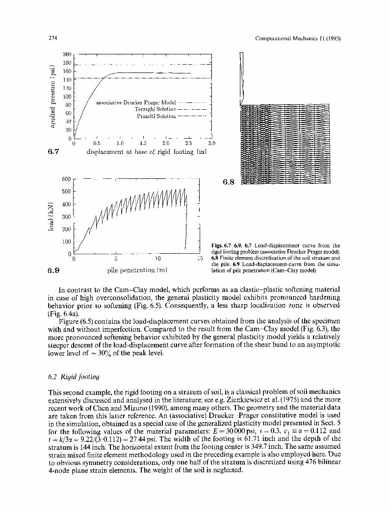
Figs. 6.7-6.9. 6.7 Load-displacement curve from the rigid footing problem (associative Drucker Prager model). 6.8 Finite element discretization of the soil stratum and the pile. 6.9 Load-displacement-curve from the simulation of pile penetration (Cam-Clay model)

In contrast to the Cam-Clay model, which performs as an elastic-plastic softening material in case of high overconsolidation, the general plasticity model exhibits pronounced hardening behavior prior to softening (Fig. 6.5). Consequently, a less sharp localization zone is observed (Fig. 6.4a).

Figure (6.5) contains the load-displacement curves obtained from the analysis of the specimen with and without imperfection. Compared to the result from the Cam-Clay model (Fig. 6.3), the more pronounced softening behavior exhibited by the general plasticity model yields a relatively steeper descent of the load-displacement curve after formation of the shear band to an asymptotic lower level of ~ 30~ of the peak level.

6.2 Rigid footin9

This second example, the rigid footing on a stratum of soil, is a classical problem of soil mechanics extensively discussed and analysed in the literature; see e.g. Zienkiewicz et al. (1975) and the more recent work of Chen and Mizuno (1990), among many others. The geometry and the material data are taken from this latter reference. An (associative) Drucker-Prager constitutive model is used in the simulation, obtained as a special case of the generalized plasticity model presented in Sect. 5 for the following values of the material parameters: E = 30000psi, v = 0.3, cl---e = 0.112 and t = k/3o~ = 9.22/(3"0.112)= 27.44 psi. The width of the footing is 61.71 inch and the depth of the stratum is 144 inch. The horizontal extent from the footing center is 349.7 inch. The same assumed strain mixed finite element methodology used in the preceding example is also employed here. Due to obvious symmetry considerations, only one half of the stratum is discretized using 476 bilinear 4-node plane strain elements. The weight of the soil is neglected.

!i~:: :"

ii ~)

~ Ni:

::i::

i

iiii:i:

==~/ii:

�9 .! ..~

~!~

i~

�9 :::.::iiii

i~ I !~

: :

�9

0 m"

P.

Oo 0

TE

NS

. V

OL.

PL.

ST

.

< 1.

000E

-03

�9

3.0

00

E-0

1

6.10

CO

MP

, V

OL.

PL.

ST

< -3

.000

E-0

2 m

>-3

.000

E-0

3

6.11

RA

DIA

L S

TR

ES

SE

S

< -2

.200

E+0

2 II �9 -1

.000

E+0

0

6.12

AX

IAL

ST

RE

SS

ES

< -1

.20

0E

§

�92

47

Fig

s. 6

.10-

6.12

. 6.

10 D

istr

ibu

tion

of

plas

tic

volu

met

ric

tens

ile

stra

ins

(lef

t h

and

sid

e) a

nd

com

pres

sive

st

rain

s (r

ight

han

d s

ide)

in t

he d

efor

med

con

- fi

gura

tion

at

u

= 2.

0m,

8.0m

an

d

13.6

m. 6

.11

Dis

trib

uti

on o

f com

pre

s-

sive

rad

ial

stre

sses

in

the

defo

rmed

co

nfig

urat

ion

at u

= 2

.0 m

, 8,

0 m

an

d

13.6

m. 6

.12

Dis

trib

uti

on o

f com

pre

s-

sive

ax

ial

stre

sses

in

th

e de

form

ed

conf

igur

atio

n at

u =

2.0

m,

8.0

m a

nd

13

.6m

L/I


Figure 6.6 shows the computed distribution of the equivalent plastic strains gP and the velocity field in the deformed configuration of the stratum at a settlement of 2.5 inches. Observe the massive concentration of plastic strains in the vicinity of the corner of the footing (gP > 40~o!) and, in particular, the narrow slip-line shaped zone of plastification, emanating from this corner. Figure 6.7 shows the load-displacement curve, with the load being related to the area under the footing. The numerically predicted collapse load, p, = 156.3 psi is higher than the classical Prandtl solution (143 psi) and lower than the Terzaghi solution (175 psi). (The values for p, obtained by Zienkiewicz et al. and by Chen and Mizuno are 151 psi and 171 psi, respectively).

6.3 Pile penetration in soil

As a final example we consider the quasi-static, axisymmetric simulation of a pile penetration in soil, under the assumption of drained conditions. This type of problems clearly involves large deformations and finite strains. The soil is assumed to be normally consolidated Weald Clay, represented by the modified Cam-Clay model.

The same model parameters employed in the preceding examples are also used here; i.e.: 2 = 0.088, x = 0.031, N = 2.097, M = 0.882, G = 3000kPa. The preconsolidation pressure is t = q0 = 87 kPa, along with a threshold value qmin = 20 kPa such that q > qmin. The finite element mesh is as depicted in Fig. 6.8. The cylindrical stratum of soil (radius r = 22.4 m, height h -- 20.7 m) is discretized by 960 axisymmetric crossed-triangles. The pile (radius r = 0.88 m, total length l = 13.8 m, length of the vertical shaft l = 12.05 m) is assumed to be rigid. The horizontal displacement boundary conditions at the remote boundary of the stratum are assumed fixed. The "centerline', which has to be given a hypothetical small thickness, as well as the pile are treated as rigid obstacles within the deformable soil. The contact constraints are enforced using an augmented lagrangian technique with frictionless contact assumed at the interface between the soil and the pile. We remark, however, that the consideration of friction does not pose any additional difficulties, and we refer to Simo and Laursen (1991) for a detailed description concerning the augmented lagrangian treatment of contact problems involving friction. The normal and tangential penalties have been chosen as ~N = 109 and ~r = 109, respectively. 200 time steps were used per 1 meter pile advancement.

Figure 6.9 shows the load-displacement curve obtained from the penetration analysis. The zig-zag form of the curve is induced by the relatively coarse mesh used in the simulation and caused by the periodical release of nodal forces whenever a node loses contact with the inclined surface (cone) of the pile. The numerically predicted maximal load at the end of the pile installation is 516 kN, the corresponding cone pressure is 212.1 kPa. Figures 6.10a-c show the distribution of volumetric plastic strains at 3 different stages of the penetration process: u = 2 m, u = 8 m and u = 13.6 m. The left hand side contains tensile, the right hand side compressive plastic volumetric strains. In the immediate vicinity of the pile, very large tensile plastic strains, connected with considerable softening of the material adjacent to the pile, are induced during the process of pile stallation. Qualitatively, this behavior is in good agreement with field observations. Quantitatively, however, the physical relevance of the numerical predictions in this narrow zone may be question- able, since the predictive capability of the Cam-Clay model on the supercritical side is rather limited (see, for instance Wood 1990). Figure 6.11 contains contour-plots of the compressive radial, Fig. 6.12 of the compressive axial stresses in the three above-mentioned stages of the penetration. A concentration of compressive axial stresses is observed beneath the cone, high compressive radial stresses are induced within ~ 3 times of the pile radius lateral to the inclined surface of the cone. The white shaded zone adjacent to the shaft of the pile again illustrates the severe softening due to remolding of the soil.

7 Concluding remarks

The methodology described in the preceding sections allows the generalization of any (isotropic) model of infinitesimal plasticity to the regime of finite strains. As already pointed out, this extension


preserves the form of the yield condition, now formulated in therms of true stresses, and retains the hyperelastic character of the stress-strain relations. The exponential approximation described in Sect. 3 possesses the remarkable property of preserving both the structure and algorithmic moduli of the now standard return mapping algorithms, now reformulated in principal Eulerian axes. An element of novelty in the application of the preceding methodology to the modified Cam-Clay model concerns the formulation of semi-explicit integration schemes. This alternative approach retains the unconditional stability property associated with an implicit treatment of the flow rule, while achieving symmetry of the algorithmic moduli via an explicit integration of the hardening law.

The general class of single surface phenomenological plasticity models for granular materials presented in Sect. 5 is applicable to a number of different geologic materials, including sands, cohesive soils and rocks. This unified treatment encompasses Most of the standard phenomenological plasticity models as special cases. In particular, J2-flow theory, Drucker-Prager and modified Cam-Clay. The restriction to isotropy is the direct result of formulating the yield criterion in terms of true stresses. We remark that nonlinear isotropic and kinematic hardening rules fit within this framework.

The nonlinear finite element simulations presented in Sect. 6 demonstrate the general applicability of the proposed algorithmic treatment of classical plasticity by means of three rather different and representative geomechanical problems. An analysis of shear band formation in soil specimen, a rigid footing problem and the simulation of pile penetration in soil.

Acknowledgements

Support for this research was partially provided by DNR via a contract with the Port Huaneme Naval Civil Engineering Laboratory. G. Meschke was supported by the MAX KADE Foundation under Grant No. 2-DJA-616 with Stanford University. This support and the interest of Dr. J. Malvar and Dr. T. Shugar are gratefully acknowledged.

References

Borja, R. I. (1991): Cam-Clay Plasticity. Part II: Implicit integration of constitutive equation based on a nonlinear elastic stress predictor. Comput. Meth. Appl. Mech. Eng. 20, 225 240

Borja, R. I.; Lee, S. R. (1990): Cam Clay Plasticity. Part I: Implicit integration ofelasto plastic constitutive relations. Comput. Meth. Appl. Mech. Eng. 78, 49 72

Chen, W. F..; Mizuno, E. (1990): Nonlinear analysis in soil mechanics-theory and implementation. Devel. Geotech. Eng. 53

Desai, C. S.; Somasundaram, S.; Frantziskonis, G. (1986): A hierarchical approach for constitutive modeling of geologic materials. Int. J. Num. Meth. Eng. 10, 225-257

Frantziskonis, G.; Desai, C. S.; Somasundaram, S. (1986): Constitutive model for nonassociative behavior. J. Eng. Mech. 112, 9, 932-946

Hill, R. (1950): The mathematical theory of plasticity. Dover editions, U.K. Lade, P. V.; Kim, M. K. (1988): Single hardening consistitutive model for frictional materials II. Yield criterion and plastic

work contours. Comput. Geotech. 6, 13-29 Lerov, Y.; Ortiz, M. (1989): Finite element analysis of strain localization in frictional materials. Int. J. Num. Anal. Meth.

Geomech. 13, 53-74 Luenberger, D. G. (1984): Linear and nonlin6ar programming. Addison Wesley, Menlo Park Maenchen, G.; Sacks, S. (1964): The tensor code, in methods of computational physics, 3, 181-210. B. Alder, S. Fernback

and M. Rotenberg Editors. New York: Academic Press Moreau, J. J. (1977): Evolution problem associated with a moving convex set in a hilbert space. J. Diff. Eq. 26, 347 Oliver, J. (1989): A consistent characteristic length for smeared cracking models. Int. J. Num. Anal. Meth. Eng. 28, 461-474 Ortiz, M.; Leroy, Y.; Needleman, A. (1987): A finite element method for localized failure analysis. Comput. Meth. Appl. Mech.

Eng. 61,189-214 Ortiz, M.; Simo, J. C. (1986): An analysis of a new class of integration algorithms for elastoplastic constitutive relations.

Int. J. Num. Meth. Eng. 23, 353-366 Roscoe, K. H.; Burland, J. B. (1968): On the generalized stress strain behavior of'wet' clay. In: Heyman, J.; Leckie, F. A., (eds.)

Engineering plasticity. Cambridge University Press, 535-609 Simo, J. C.; Taylor, R. L. (1985): Consistent tangent operators for rateindependent elastoplasticity. Comput. Meth. Appl. Mech.

Eng. 48, 101-118 Simo, J. C.; Ju, J.; Pister, K. S.; Taylor, R. U (1988): Assessment of cap model: Consistent return algorithms and rate-dependent

extension. J. Eng. Mech. 114, 2, 191-218


Simo, J. C. (1988): A framework for finite strain elastoplasticity based on the multiplicative decomposition and hyperelastic relations. Part I: Formulation and Part II: Computational aspects. Comput. Meth. Appl. Mech. Eng. 66, No. 2, 199-219 and 66, No. 3, 1-31

Simo, J. C.; Kennedy, J. G.; Govindjee, S. (1988): Non-smoth multisurface plasticity and viscoplasticity. Loading/unloading conditions and numerical algorithms. Int. J. Num. Meth. Eng. 26, 2161-2185

Simo, J. C.; Rifai, M. S. (1990): A class of mixed assumed strain methods and the method of incompatible modes. Int. J. Num. Meth. Eng. 29, 1595-1638

Simo, J. C.; Taylor, R. L. (1991): Finite elasticity in principal stretches; formulation and finite element implementation. Comput. Meth. Appl. Mech. Eng. 85, 273-310

Simo, J. C.; Miehe, C. (1991): Coupled associative thermoplasticity at finite strains. Formulation, numerical analysis and implementation. Comput. Meth. Appl. Mech. Eng. 98, 41-104

Simo, J. C. (1991a): Nonlinear stability of the time discrete variational problem in nonlinear heat conduction and elastoplasticity. Comput. Meth. Appl. Mech. Eng. 88, 111-131

Simo, J. C. (1991b): Algorithms for multiplicative plasticity which preserve the structure of the classical return mappings of the infinitesimal theory, SUDAM report No. 91-4. In press in comput. Meth. Appl. Mech. Eng.

Simo, J. C.; Hughes, T. J. R. (1991): Plasticity viscoplasticity and viscoelasticity: formulation and numerical analysis aspects, Springer-Verlag (in press)

Simo, J. C.; Armero, F. (1991): Geometrically nonlinear enhanced strain method and the method of incompatible modes. Int. J. Num. Meth. Eng. 33, 1413-1449

Simo, J. C.; Laursen, T. A. (1991): An augmented lagrangian treatment of contact problems involving friction. Computers and Structures, 42, No. 1, 97-116

Vardoulakis, I.; Goldscheider, M.; Gudehus, G. (1978): Formation of shear bands in sand bodies as a bifurcation problem. Int. J. Num. Anal. Meth. Geomech. 2, 99 128

Wood, D. M. (1990): Soil behavior and critical state soil mechanics. Cambridge University Press Wilkins, M. L. (1964): Calculation of elastic-plastic flow in Meth. Comput. Phys. 3, 211 272. B. Alder, S. Fernback and M.

Rotenberg editors. New York: Academic Press Zienkiewicz, O. C.; Humphenson, C.; Lewis, R. W. (1975): Associated and nonassociated viscoplasticity and plasticity in soil

mechanics. G6otechnique 25, 671-689

Communicated by S. N. Atluri, February 18, 1992

Documents

A new class of algorithms for classical plasticity extended to