Classical Elasticity and Plasticity · Classical Elasticity and Plasticity 2.1 Elasticity Fung (1965) provides elegant definitions for the different forms of elasticity theory, and

Chapter 2

Classical Elasticity and Plasticity

2.1 Elasticity

Fung (1965) provides elegant definitions for the different forms of elasticity theory, and we follow his terminology here. A material is said to be elastic if the stress can be expressed as a single-valued function of the strain:

( )ij ij ijfσ = ε (2.1)

where ( )ij ijf ε is a second-order tensor-valued function of the strains. If

( )ij ijf ε is linear in εij , then it can be written ( )ij ij ij ijkl klf dσ = ε = ε , where ijkld

is a fourth-order tensor constant usually called the stiffness matrix: this is the common case of linear elasticity. The incremental stress-strain relationship for an elastic material is written

( )ij ij

ij klkl

f∂ εσ = ε

∂ε (2.2)

Alternatively, if the stress-strain relationship is originally expressed in incre-mental form, the material is described as hypoelastic:

( ),ij ijkl ij ij klfσ = ε σ ε (2.3)

where ( ),ijkl ij ijf ε σ is a fourth-order tensor valued function of the strains or

of the stresses, or even (rarely) of both. Note that we distinguish between the fourth-order tensor function ijklf and the second-order tensor function

ijf . If ( ),ijkl ij ijf ε σ is a constant, then the material is linear elastic and

( ),ijkl ij ij ijklf dε σ = .

14 2 Classical Elasticity and Plasticity

Alternatively, if the stresses can be derived from a strain energy potential, then the material is said to be hyperelastic:

( )ij

ijij

f∂ εσ =

∂ε (2.4)

in which ( )ijf ε is a scalar valued function of the strains. (Again note that we

distinguish the scalar function f from the two tensor functions ijf and ijklf ).

It follows that

( )2

ijij kl

ij kl

f∂ εσ = ε

∂ε ∂ε (2.5)

If ( )ijf ε is a quadratic function of the strains, then the material is linear elas-

tic, and ( )2

ijijkl

ij kl

fd

∂ ε=

∂ε ∂ε.

Example 2.1 Linear Isotropic Elasticity

The following strain energy function can be used to express linear isotropic elasticity in hyperelastic form:

3 26 2

ii jj ij ijf K G

′ ′ε ε ε ε= + (2.6)

where K is the isothermal bulk modulus and G is the shear modulus. Differ-entiating the above1 gives the elastic form,

( ) 2ij ij ij kk ij ijij

ff K G

∂ ′σ = = ε = ε δ + ε∂ε (2.7)

Differentiating once more leads to the hyperelastic incremental form,

2

2ij kl ijkl kl kk ij ijij kl

fd K G

∂ ′σ = ε = ε = ε δ + ε∂ε ∂ε

(2.8)

from which one can derive

22

3ijkl ij kl ik jlG

d K G⎛ ⎞= − δ δ + δ δ⎜ ⎟⎝ ⎠

(2.9)

1 See table B.1 in Appendix B for some differentials of tensor functions.

2.1 Elasticity 15

Comparison of Equations (2.1) and (2.4) reveals that every hyperelastic mate-

rial is also elastic, with ( ) ( )ijij ij

ij

ff

∂ εε =

∂ε. Conversely, however, an elastic mate-

rial is hyperelastic only if ( )ij ijf ε is an integrable function of the strains.

Similarly, comparison of Equations (2.2) and (2.3) reveals that all elastic ma-

terials are also hypoelastic, with ( ) ( ),

ij ijijkl ij ij

kl

ff

∂ εε σ =

∂ε. Again, the converse is

not true, and a hypoelastic material is elastic only if ( ),ijkl ij ijf ε σ can be ex-

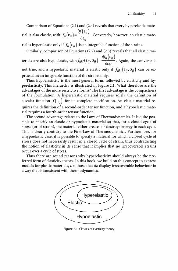
pressed as an integrable function of the strains only. Thus hypoelasticity is the most general form, followed by elasticity and hy-

perelasticity. This hierarchy is illustrated in Figure 2.1. What therefore are the advantages of the more restrictive forms? The first advantage is the compactness of the formulation. A hyperelastic material requires solely the definition of a scalar function ( )ijf ε for its complete specification. An elastic material re-

quires the definition of a second-order tensor function, and a hypoelastic mate-rial requires a fourth-order tensor function.

The second advantage relates to the Laws of Thermodynamics. It is quite pos-sible to specify an elastic or hypoelastic material so that, for a closed cycle of stress (or of strain), the material either creates or destroys energy in each cycle. This is clearly contrary to the First Law of Thermodynamics. Furthermore, for a hypoelastic case, it is possible to specify a material for which a closed cycle of stress does not necessarily result in a closed cycle of strain, thus contradicting the notion of elasticity in its sense that it implies that no irrecoverable strains occur over a cycle of stress.

Thus there are sound reasons why hyperelasticity should always be the pre-ferred form of elasticity theory. In this book, we build on this concept to express models for plastic materials, i. e. those that do display irrecoverable behaviour in a way that is consistent with thermodynamics.

Hypoelastic

ElasticHyperelastic

Figure 2.1. Classes of elasticity theory


2.2 Basic Concepts of Plasticity Theory

Before moving on to the new formulation of plasticity theory that is the main subject of this book, it is useful to present the conventional formulation of plas-ticity theory. This serves as a basis for comparison for the approach presented in later chapters.

The first and fundamental assumption of plasticity theory is that the strains can be decomposed into additive elastic and plastic components:

( ) ( )e pij ij ijε = ε + ε (2.10)

The elastic strains ( )eijε can be specified by any of the means used for elasticity,

as discussed in Section 2.1 . For the reasons described there, the hyperelastic approach would of course be preferred. The changes of elastic strain are thus solely related to changes in stress.

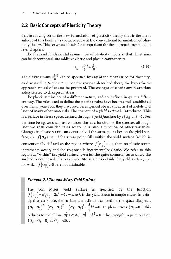
The plastic strains are of a different nature, and are defined in quite a differ-ent way. The rules used to define the plastic strains have become well established over many years, but they are based on empirical observation, first of metals and later of many other materials. The concept of a yield surface is introduced. This is a surface in stress space, defined through a yield function by ( ), 0ijf σ =… . For

the time being, we shall just consider this as a function of the stresses, although later we shall consider cases where it is also a function of other variables. Changes in plastic strain can occur only if the stress point lies on the yield sur-face, i. e. ( ) 0ijf σ = . If the stress point falls within the yield surface (which is

conventionally defined as the region where ( ) 0ijf σ < ), then no plastic strain

increments occur, and the response is incrementally elastic. We refer to this region as “within” the yield surface, even for the quite common cases where the surface is not closed in stress space. Stress states outside the yield surface, i. e. for which ( ) 0ijf σ > , are not attainable.

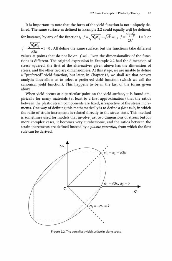
Example 2.2 The von Mises Yield Surface

The von Mises yield surface is specified by the function

( ) 22 0ij ij ijf k′ ′σ = σ σ − = , where k is the yield stress in simple shear. In prin-

cipal stress space, the surface is a cylinder, centred on the space diagonal,

( ) ( )221 2 2 3σ − σ + σ − σ ( )2 2

3 13

02

k+ σ − σ − = . In plane stress ( )2 0σ = , this

reduces to the ellipse 2 2 21 1 3 3 3 0kσ + σ σ + σ − = . The strength in pure tension

( )2 3 0σ = σ = is 1 3kσ = .

2.2 Basic Concepts of Plasticity Theory 17

It is important to note that the form of the yield function is not uniquely de-fined. The same surface as defined in Example 2.2 could equally well be defined,

for instance, by any of the functions, 2 0ij ijf k′ ′= σ σ − = , 2

1 02

ij ijf

k

′ ′σ σ= − = or

1 02

ij ijf

k

′ ′σ σ= − = . All define the same surface, but the functions take different

values at points that do not lie on 0f = . Even the dimensionality of the func-tions is different. The original expression in Example 2.2 had the dimension of stress squared, the first of the alternatives given above has the dimension of stress, and the other two are dimensionless. At this stage, we are unable to define a “preferred” yield function, but later, in Chapter 13, we shall see that convex analysis does allow us to select a preferred yield function (which we call the canonical yield function). This happens to be in the last of the forms given above.

When yield occurs at a particular point on the yield surface, it is found em-pirically for many materials (at least to a first approximation) that the ratios between the plastic strain components are fixed, irrespective of the stress incre-ments. One way of defining this mathematically is to define a flow rule, in which the ratio of strain increments is related directly to the stress state. This method is sometimes used for models that involve just two dimensions of stress, but for more complex cases, it becomes very cumbersome, and the ratios between the strain increments are defined instead by a plastic potential, from which the flow rule can be derived.

k=σ−=σ 31

k331 =σ=σ

0,3 31 =σ=σ k

Figure 2.2. The von Mises yield surface in plane stress


The plastic potential, like the yield surface, is a function of the stresses and other variables, and is usually written ( ), 0ijg σ =… . The direction of the plastic

strain increment is then defined as normal to the plastic potential:

( ) ( )ijpij

ij

g∂ σε = λ

∂σ (2.11)

where λ is a plastic multiplier which is as yet undetermined. In metal plasticity, it is usual for the yield function ( ), 0ijf σ =… and the

plastic potential ( ), 0ijg σ =… to be identical functions. This choice is based

both on a wealth of empirical evidence and also on sound theoretical grounds (see Section 2.5 ). This important case is called “associated flow” or “normality” (in the sense that the plastic strain increments are normal to the yield surface, and not in the sense that “normal” means that this represents the usual behav-iour of materials). There are many advantages of theories that adopt associated flow, sufficient that many practitioners go to elaborate means to avoid using non-associated flow theories. However, for some materials, notably soils, the empirical evidence for non-associated flow is so overwhelming that it is essential to address this more complex case.

It is usual (although not essential) to define the plastic potential so that 0g = at the particular stress point at which the strain increment is required. This means that (except for associated flow) it is necessary to introduce some addi-tional dummy variables, say x, into the plastic potential, defined so that

( ), 0ijg xσ = at the particular stress point on the yield surface.

Note that we follow here the common notation in plasticity theory and use f for the yield function and g for the plastic potential. Later in this book, we shall need to use f and g for the Helmholtz and Gibbs free energies, as is common practice in thermodynamics. We shall attempt to make the meaning of the vari-ables clear whenever there is any danger of ambiguity.

The yield surface defines the possibility of plastic strain increments, and the plastic potential then defines the ratios between the plastic strain increments; but what remains to be defined is the magnitude of the plastic strains. It is in this area that the greatest variety of ways of specifying plasticity models is found, and it is not possible to present an approach that encompasses all the different forms in the literature.

Apart from perfectly plastic materials (see Section 2.3 below), the magnitude of plastic strain is defined by establishing a link between the plastic strains and the expansion (or movement or contraction) of the yield surface. Probably the most common approach is to define the yield surface so that it is a function of the stresses and some hardening parameters ξ, which are usually scalars, but could be tensors. Thus the yield surface is written ( ), 0ijf σ ξ = . The hardening pa-

rameters are, in turn, defined in terms of the plastic strains. The most common

2.3 Incremental Stiffness in Plasticity Models 19

form is that the hardening parameters are simply functions of the plastic strains ( )( )ξ ξ ε pij= . In this case, the hardening parameters can be eliminated from the

formulation and the yield function simply expressed in the form ( )( )σ ε =, 0p

ij ijf .

This form of hardening is called strain hardening. An alternative is that, although the hardening parameters cannot be ex-

pressed as functions of the plastic strains, evolution equations can be defined for the hardening parameters in terms of the plastic strain rates. The evolution equations may also involve other variables, so that a rather general form is

( ) ( )( )ξ = ξ σ ε ξ ε, , ,p pij ij ij (2.12)

(We hesitate to say that the above is the most general possible form because the imagination of plasticity theorists in devising ever more complex approaches seems almost boundless.) One important special case occurs when ξ is identified

with plastic work, in which case we can write ( ) ( )ppij ijWξ = = σ ε . The term work

hardening is strictly applicable only to this case, although it is frequently applied much more loosely to any hardening process.

To recapitulate, a strain hardening plasticity model can be completely defined by the following assumptions:

• Decomposition of the strain into elastic and plastic components;

• Definition of the elastic strains, using, for instance, a hyperelastic law that requires specification of a single scalar function;

• Definition of a yield surface ( )( )σ ε, 0pij ijf = ;

• Definition of a plastic potential ( )( )σ ε, , 0pij ijg x = .

Thus the model requires three scalar functions to be defined for its complete specification. Unfortunately, many plasticity theories do not adhere to this sim-ple pattern, and some adopt a series of ad hoc rules and assumptions. Not only can this be confusing, but it also makes comparisons between competing theories difficult. At worst, it can lead to theories that are not internally self-consistent.

2.3 Incremental Stiffness in Plasticity Models

For any constitutive model, one of the most important operations is derivation of the incremental stress-strain relationship. For plasticity theories, the method adopted is different for the special case of perfect plasticity. So we shall treat this case first, before going on to the case of hardening plasticity.


2.3.1 Perfect Plasticity

In perfect plasticity, the yield surface remains fixed in stress space, so there is no hardening (or softening). Thus the yield surface is only a function of the stress

( ) 0ijf σ = . The plastic potential will have the form ( ), 0ijg xσ = , where x are the

dummy variables introduced to satisfy the (not strictly necessary) condition that 0g = at each stress point on the yield surface. The incremental stress-strain

relationship is obtained by combining the equations below. The strain decomposition is written in incremental form:

( ) ( )e pij ij ijε = ε + ε (2.13)

The elastic strain rates are defined by a stiffness matrix:

( )eij ijkl kldσ = ε (2.14)

Note that the above form can always be derived, irrespective of whether the elastic strains are specified through hyperelasticity, elasticity, or hypoelasticity.

The yield surface is written in differential form, noting that during any proc-ess in which the plastic strains are non-zero, not only is 0f = , but also 0f = . This incremental form of the yield surface is usually referred to as the consis-tency condition:

0ijij

ff

∂= σ =∂σ (2.15)

Finally, we need the plastic strain rate ratio, obtained from the plastic potential:

( )pij

ij

g∂ε = λ∂σ (2.16)

Substituting (2.13) and (2.16) in (2.14) gives

( ) ( )( ) ⎛ ⎞∂σ = ε = ε − ε = ε − λ⎜ ⎟∂σ⎝ ⎠

e pij ijkl ijkl kl ijkl klkl kl

kl

gd d d (2.17)

Combining Equations (2.15) and (2.17), we obtain

0ij ijkl klij ij kl

f f gf d

⎛ ⎞∂ ∂ ∂= σ = ε − λ =⎜ ⎟∂σ ∂σ ∂σ⎝ ⎠ (2.18)

which leads to the solution for the plastic multiplier λ:

ijkl kl

ij

pqrspq rs

fd

f gd

∂ ε∂σ

λ = ∂ ∂∂σ ∂σ

(2.19)


Equation (2.19) is then back-substituted in (2.17) to give

mnab ab

mnij ijkl kl ijkl

klpqrs

pq rs

fd

gd d

f gd

⎛ ⎞∂ ε⎜ ⎟∂σ ∂⎜ ⎟σ = ε − ∂ ∂⎜ ⎟ ∂σ⎜ ⎟∂σ ∂σ⎝ ⎠

(2.20)

With some interchanging of the dummy subscripts, this can be rewritten

( )epij klijkldσ = ε (2.21)

where ( )epijkld is the elastic-plastic stiffness matrix defined as

( ) ijab mnklep ab mn

ijklijklpqrs

pq rs

g fd d

d df g

d

∂ ∂∂σ ∂σ= − ∂ ∂

∂σ ∂σ

(2.22)

Thus, given the specification of the elastic behaviour, the yield surface, and the plastic potential, the incremental constitutive behaviour can be obtained by applying a purely automatic process to obtain the incremental stress-strain rela-tionship. This is important because no further ad hoc assumptions are neces-sary. Note also that the derivation involves solely matrix manipulation and dif-ferentiation. Both processes can be readily carried out using symbolic manipulation packages.

Example 2.3 Von Mises Plasticity with Isotropic Elasticity

Using the yield surface as defined in Example 2.2, which is also the plastic potential as the von Mises model uses associated flow, then

22ij ijf g k′ ′= = σ σ − , so that 2ij ij ijf g ′∂ ∂σ = ∂ ∂σ = σ .

From Example 2.1, 2

23ijkl ij kl ik ilG

d K G⎛ ⎞= − δ δ + δ δ⎜ ⎟⎝ ⎠

. Noting that for this

case, ∂ ∂ ′= = σ

∂σ ∂σ4ijkl klij ij

kl kl

g fd d G , substitution in Equation (2.22) gives

( ) ′ ′σ σ⎛ ⎞= − δ δ + δ δ −⎜ ⎟ ′ ′σ σ⎝ ⎠

222

3ij klep

ij kl ik jlijklpq ij

GGd K G (2.23)

which can be further simplified to

( ) ⎛ ⎞ ′ ′= − δ δ + δ δ − σ σ⎜ ⎟⎝ ⎠ 2

22

3ep

ij kl ik jl ij klijklG G

d K Gk

(2.24)


It is important to note that this stiffness matrix is singular, so that it cannot be inverted to give a compliance matrix. This is a feature common to all perfect plasticity models.

2.3.2 Hardening Plasticity

Incremental Response for Strain Hardening

For strain-hardening plasticity, Equations (2.13), (2.14), and (2.16) take the same form, but because the yield surface is now also a function of the plastic strains, the consistency condition takes the form

( )( )∂ ∂= σ + ε =

∂σ ∂ε0

pij ijp

ij ij

f ff (2.25)

Substituting the flow rule (2.16), we obtain

( )∂ ∂ ∂= σ + λ =

∂σ ∂σ∂ε0ij p

ij ijij

f f gf (2.26)

It is more convenient in this case to obtain the solution for λ in terms of the stress increment rather than the strain increment (as was used for perfect plas-ticity):

( )

∂ σ∂σ

λ = − ∂ ∂∂σ∂ε

ijij

pijij

f

f g (2.27)

The quantity ( )∂ ∂= −

∂σ∂ε pijij

f gh is often termed the hardening modulus, and we

can write ∂λ = σ

∂σ1

ijij

fh

or ( ) ∂ ∂ε = σ∂σ ∂σ

1pklij

ij kl

g fh

. The hardening modulus is not

a defined parameter of the model, but is derived at a given stress point in terms of the yield function and plastic potential. It is identically zero in a perfect plas-ticity model.

The most convenient way to proceed is to use the elastic compliance matrix,

( )ε = σeijkl klij c (2.28)


so that

( )kl

klijklijkl

pijklijklij

fgh

cc σσ∂∂

σ∂∂−σ=ε−σ=ε 1 (2.29)

which leads immediately to ( )kl

epijklij c σ=ε , where the elastic-plastic compliance

matrix is

( ) mnpmn

klijijkl

klijijkl

epijkl gf

fg

cfgh

cc

σ∂∂

ε∂∂

σ∂∂

σ∂∂

+=σ∂∂

σ∂∂−= 1)( (2.30)

If the stiffness matrix is required, it can be obtained either by numerical in-version of the compliance matrix, or by solving for the plastic multiplier, as before, in terms of the strains. Starting with the consistency condition,

( )

( )

( ) 0=σ∂∂

ε∂∂λ+⎟⎟

⎠

⎞⎜⎜⎝

⎛σ∂∂λ−ε

σ∂∂=

εε∂∂+σ

σ∂∂=

ijpijkl

klijklij

pijp

ijij

ij

gfgdf

fff (2.31)

the solution for λ becomes

( ) rsprs

pqrspq

klijklij

gfdf

df

σ∂∂

⎟⎟

⎠

⎞

⎜⎜

⎝

⎛

ε∂

∂−σ∂∂

εσ∂∂

=λ (2.32)

The solution then proceeds exactly as for the perfectly plastic case, except that

this time ( )epijkld takes the form

( )

( ) rsprs

pqrspq

mnklmnab

ijab

ijklepijkl

gfdf

dfgddd

σ∂∂

⎟⎟

⎠

⎞

⎜⎜

⎝

⎛

ε∂∂−

σ∂∂

σ∂∂

σ∂∂

−= (2.33)

Note that if ( ) 0=ε∂∂ prsf then Equation (2.33) reduces to the result for per-

fect plasticity, (2.22). However, the equation for compliance, Equation (2.30), becomes singular in the perfectly plastic case.


Incremental Response for Work Hardening

Because of its historical importance, we set out here the particular case of work hardening, but this section can be omitted and the reader can proceed to Sec-tion 2.3.3. For work-hardening plasticity, Equations (2.13), (2.14), and (2.16)

again apply, but now we write the yield surface in the form ( )( ), 0pijf Wσ = ,

where ( ) ( )pijij

pW εσ= .

The consistency condition takes the form,

( )( ) 0=

∂

∂+σσ∂∂= p

pijij

WWfff (2.34)

Substituting the definition of the plastic work and the flow rule (2.16), we obtain

( ) 0=σ∂∂σ

∂∂λ+σ

σ∂∂=

ijijpij

ij

gWfff (2.35)

so that

( ) ijijp

ijij

gWf

f

σ∂∂σ

∂∂

σσ∂∂

−=λ (2.36)

and recalling that klklij

pij

fgh

σσ∂∂

σ∂∂=ε 1)(

, the hardening modulus in this case

is ( ) ijijp

gWfh

σ∂∂σ

∂∂−= .

The analysis proceeds exactly as for the strain hardening case, except that this time

( ) mnmnp

klijijkl

klijijkl

epijkl g

Wf

fg

cfgh

cc

σ∂∂σ

∂∂

σ∂∂

σ∂∂

+=σ∂∂

σ∂∂−= 1)( (2.37)


The alternative analysis for the stiffness matrix starts with the consistency condition,

( )

( )

( ) 0=σ∂∂σ

∂

∂λ+⎟⎟⎠

⎞⎜⎜⎝

⎛σ∂∂λ−ε

σ∂∂=

∂

∂+σσ∂∂=

ijijpkl

klijklij

ppij

ij

gWfgdf

WWfff

(2.38)

and the solution for λ becomes

( ) rsrsppqrs

pq

klijklij

gWfdf

df

σ∂∂

⎟⎟⎠

⎞⎜⎜⎝

⎛σ

∂∂−

σ∂∂

εσ∂∂

=λ (2.39)

Again, the solution proceeds as before, and this time ( )epijkld takes the form

( )

( ) rsrsppqrs

pq

mnklmnab

ijab

ijklepijkl

gWfdf

dfgddd

σ∂∂

⎟⎟⎠

⎞⎜⎜⎝

⎛σ

∂

∂−σ∂∂

σ∂∂

σ∂∂

−= (2.40)

2.3.3 Isotropic Hardening

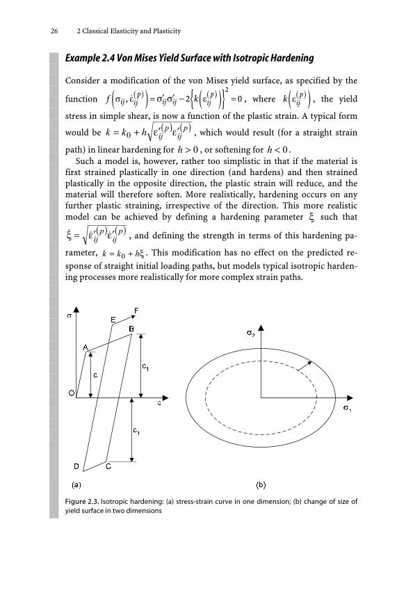
If, the yield surface expands (or contracts) but does not translate as plastic straining occurs, then this is said to be isotropic hardening (or softening). This is illustrated in Figure 2.3a for a simple one-dimensional material that hardens linearly and isotropically with plastic strain. The material yields at A at a stress c, and during plastic deformation AB, it hardens and the stress increases to 1c . It is then unloaded, and reverse yielding occurs at C when the stress is − 1c . Further hardening occurs on CD, so that, when the material is reloaded, the expansion of the yield surface is such that the yield at E occurs above the original curve AB, and further hardening occurs along EF.

Figure 2.3b illustrates isotropic hardening in two dimensions. The surface ex-pands but does not change shape.


Example 2.4 Von Mises Yield Surface with Isotropic Hardening

Consider a modification of the von Mises yield surface, as specified by the

function ( )( ) ( )( ){ }σ ε ε2

, 2 0p pij ij ijij ijf k′ ′= σ σ − = , where ( )( )ε p

ijk , the yield

stress in simple shear, is now a function of the plastic strain. A typical form

would be ( ) ( )pij

pijhkk ε′ε′+= 0 , which would result (for a straight strain

path) in linear hardening for 0>h , or softening for 0<h . Such a model is, however, rather too simplistic in that if the material is

first strained plastically in one direction (and hardens) and then strained plastically in the opposite direction, the plastic strain will reduce, and the material will therefore soften. More realistically, hardening occurs on any further plastic straining, irrespective of the direction. This more realistic model can be achieved by defining a hardening parameter ξ such that

( ) ( )pij

pij ε′ε′=ξ , and defining the strength in terms of this hardening pa-

rameter, ξ+= hkk 0 . This modification has no effect on the predicted re-

sponse of straight initial loading paths, but models typical isotropic harden-ing processes more realistically for more complex strain paths.

Figure 2.3. Isotropic hardening: (a) stress-strain curve in one dimension; (b) change of size of yield surface in two dimensions


2.3.4 Kinematic Hardening

On the other hand, if the yield surface translates, but does not change size, as plastic strain occurs, then this is said to be kinematic hardening. Figure 2.4a, which should be contrasted with Figure 2.3a, shows the response of a simple kinematic hardening material that hardens linearly with plastic strain. The load-ing curve OAB is identical to that of isotropic hardening, but on unloading from B, yield occurs at C′ , such that the size of the elastic region is 2c (the stress at C′ therefore is −1 2c c ). Hardening occurs on reverse loading C D′ ′ , but on reload-ing, yield occurs at E′ , which falls on the original line AB, and the hardening once again occurs along E F′ ′ .

Figure 2.4b (which should be contrasted with Figure 2.3b) shows the transla-tion of a yield surface for a kinematic hardening model in two dimensions.

Figure 2.4. Kinematic hardening (a) stress-strain behaviour in one dimension; (b) translation of yield surface in two dimensions

Example 2.5 Von Mises Yield Surface with Kinematic Hardening

Consider a modification of the von Mises yield surface, specified by the func-

tion ( )( ) ( )( ) 2, 2 0pij ij ij ij ij ijf k′ ′ ′ ′σ ε = σ − ρ σ − ρ − = , where

( )( )pij ij ij′ ′ρ = ρ ε , called

the back stress, is a function of the plastic strain. A simple form would be ( )p

ij ijh '′ρ = ε , which would result (for a straight strain path) in linear harden-

ing. This hardening relationship could also be written ( )′ ′ρ = ε p

ij ijh , so that the

translation of the yield surface is in the same direction as the direction of


the plastic strain. This type of hardening is often referred to as Prager’s trans-lation rule. Alternatively, one could write ( )ijijij ρ′−σ′μ=ρ′ , where μ is a

scalar multiplier, so that the translation of the yield surface is in the same direction as ( )ijij ρ′−σ′ . This is often known as Ziegler’s translation rule. For

the special case of the von Mises type of yield surface with associated flow, the

two translation rules are identical: ( )ijijij

ijij hghh ρ′−σ′λ=σ′∂∂λ=ε′=ρ′ 2 .

2.3.5 Discussion of Hardening Laws

It is impossible to distinguish between kinematic and isotropic hardening if one considers only the plastic behaviour of materials during initial monotonic load-ing, as illustrated by curves OAB in Figures 2.3a and 2.4a. It is during unloading and subsequent reloading that the differences between the theories are exhib-ited. During isotropic hardening, the elastic region changes its size but not shape, whereas during pure kinematic hardening, it translates but does not change size (Figure 2.3b and 2.4b). Some materials exhibit one type of behaviour whilst others exhibit the other. For instance, the very successful “critical state” family of models for the behaviour of soft clays uses isotropic hardening. In these models, hardening is linked to volumetric strain rather than shear strain, and this concept proves vitally important in modelling geotechnical materials.

On the other hand, an important extension of kinematic hardening (pursued in detail in Chapter 7) allows the modelling of “Masing” type of hysteretic behav-iour, and this proves realistic for many cyclic loading applications. Of course, mixed forms of hardening, involving both expansion and translation of the yield surface are also employed, for instance, in modelling the behaviour of soils under complex loading paths. Further discussion of different types of hardening in some more recent developments of plasticity theory is given in Chapter 6.

Finally, there is the possibility that the yield surface changes shape as well as its size or location. Some advanced theories for soils employ yield surfaces which change shape; see, for example, Whittle (1993).

2.4 Frictional Plasticity

We shall return later in Chapter 10 to the more realistic modelling of frictional materials, but it is useful at this stage to introduce some of the simple concepts of fricional plasticity, as this is the most important application in which non-associated flow occurs. We consider a simple conceptual model in which a mate-rial is subjected to a normal stress σ and a shear stress τ , with corresponding strains ε and γ . If the material had a cohesive strength c (independent of the normal stress) and exhibited associated flow, we could write the yield surface

2.4 Frictional Plasticity 29

and plastic potential as 0=−τ== cgf . It is straightforward to show that

(since 0=σ∂∂g ) this model involves plastic flow at constant volume. Note that in the following discussion of friction, we maintain our usual con-

vention of tensile positive. Those readers more familiar with the compressive positive terminology used in frictional problems in soil mechanics will need to take special care.

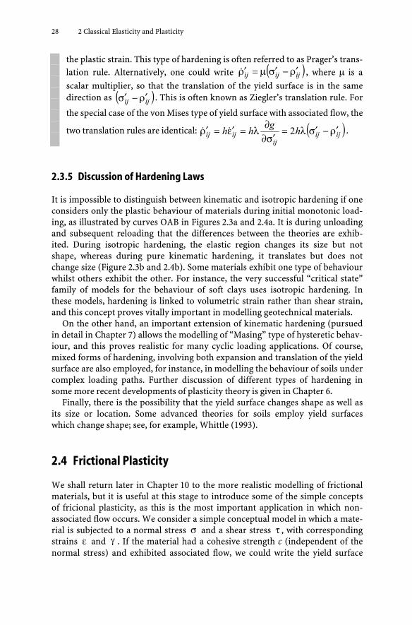
The yield surface for a perfectly plastic frictional can be defined as

= τ + μ σ =* 0f (2.41)

where μ∗ is the apparent coefficient of internal friction. We note that for this frictional material, the stress σ will always be negative (i. e. compressive). Within the yield surface, the stress-strain behaviour is elastic and could be written

σεK

= τγG

= (2.42)

During plastic flow, the stress-strain behaviour is governed by the flow rule:

( )ε λσ

p g∂=∂

( )γ λτ

p g∂=∂

(2.43)

where g is the plastic potential, which we write in the form,

0=−βσ+τ= xg (2.44)

where β is a coefficient which we discuss below, and x is a constant chosen to ensure that the plastic potential surface always passes through the current stress state on the yield surface.

Clearly, if β = μ*, then the yield surface and plastic potential are identical and the flow rule (2.43) becomes associated. In this case, it follows from (2.43) that

( )ε λ λμ*p = β = and ( ) ( )γ λSp = τ [See the notation section for the definition of the signum function S(x)]. The rate of plastic work is then determined as

( ) ( ) ( ) ( ) ( )* S *p p pW = σε + τγ = λμ σ + λτ τ = λ μ σ + τ , and by substituting the

expression for the yield surface, we obtain ( ) 0pW = . Thus a “frictional” mate-rial with associated flow is not frictional at all. It dissipates no work plastically!

Now consider plastic strains in more detail. It is simple to show from the flow

rule that ( ) ( ) ( )ε γ βS τp p = . Since λ is a positive multiplier, it also follows that

τ and ( )pγ have the same sign, so that we can write ( ) ( ) ( )( )ε γ β γSp p p= or

( ) ( )p pε = β γ . For a positive value of β, the volumetric plastic strain is always

positive and the material dilates. The apparent “frictional” strength in an associ-ated material is entirely due to this dilation. More realistically, *β < μ and


( ) ( ) ( )*pW = λ βσ + τ = −λσ μ −β , which is positive because 0σ < , so that plastic work is dissipated in this case. The case β > μ * would generally be disallowed

on “thermodynamic” grounds as this would involve negative plastic work. It is common to identify plastic work with thermodynamic dissipation. We shall see later in this book that this is in general an oversimplification, but in this in-stance, the identification of plastic work with dissipation is correct.

For 0β = , ( ) 0pε = , and the material deforms at constant volume. The yield surface and flow vectors for the general case are shown in Figure 2.5.

2.5 Restrictions on Plasticity Theories

In the discussion of frictional materials, we have just encountered the fact that certain restrictions may be placed on parameters on “thermodynamic” grounds. Two important restrictions on plasticity theories have been applied by many

Figure 2.5. Frictional yield surface

2.5 Restrictions on Plasticity Theories 31

users in the past, and these are discussed below. Both bear a superficial similarity to thermodynamic laws, and both lead to normality relationships, but neither embodies any thermodynamic principles.

2.5.1 Drucker's Stability Postulate

Drucker (1951) proposed a “stability postulate” for plastically deforming mate-rials. Although not a thermodynamic statement, it bears a passing resemblance to the Second Law of Thermodynamics and is therefore referred to as a “quasi-thermodynamic” postulate for classifying materials. It can be stated in a variety of equivalent ways, but represents the idea that, if a material is in a given state of stress and some “external agency” applies additional stresses, then “The work done by the external agency on the displacements it produces must be positive or zero” (Drucker, 1959). If the external agency applies a stress increment δσij

that causes additional strains δεij , then the postulate is that δσ δε ≥ 0ij ij . The

product δσ δεij ij is often called the second order work.

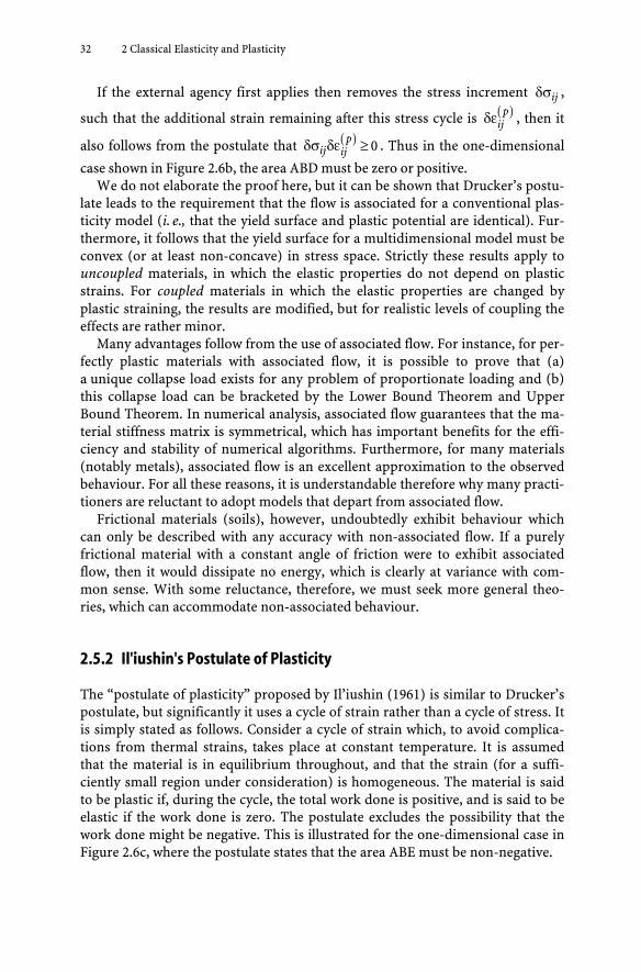
In the one-dimensional case shown in Figure 2.6a, the postulate states that the area ABC must be positive. Strain-softening behaviour is thus excluded. In the one-dimensional case, a strain-softening material is mechanically unstable un-der stress control, and this is linked to the identification of the postulate as a “stability postulate”. Unfortunately, this has led to the interpretation that a material which does not obey the postulate will exhibit mechanically unstable behaviour. The obvious corollary is that a material which is mechanically stable must therefore obey the postulate. The identification of the postulate with me-chanical stability for the multidimensional case is, however, erroneous. The conclusion that mechanically stable materials must obey Drucker’s postulate is therefore equally erroneous.

Figure 2.6. One-dimensional illustrations of (a,b) Drucker’s postulate and (c) Il’iushin’s postulate


If the external agency first applies then removes the stress increment δσij ,

such that the additional strain remaining after this stress cycle is ( )δε pij , then it

also follows from the postulate that ( )δσ δε ≥ 0pij ij . Thus in the one-dimensional

case shown in Figure 2.6b, the area ABD must be zero or positive. We do not elaborate the proof here, but it can be shown that Drucker’s postu-

late leads to the requirement that the flow is associated for a conventional plas-ticity model (i. e., that the yield surface and plastic potential are identical). Fur-thermore, it follows that the yield surface for a multidimensional model must be convex (or at least non-concave) in stress space. Strictly these results apply to uncoupled materials, in which the elastic properties do not depend on plastic strains. For coupled materials in which the elastic properties are changed by plastic straining, the results are modified, but for realistic levels of coupling the effects are rather minor.

Many advantages follow from the use of associated flow. For instance, for per-fectly plastic materials with associated flow, it is possible to prove that (a) a unique collapse load exists for any problem of proportionate loading and (b) this collapse load can be bracketed by the Lower Bound Theorem and Upper Bound Theorem. In numerical analysis, associated flow guarantees that the ma-terial stiffness matrix is symmetrical, which has important benefits for the effi-ciency and stability of numerical algorithms. Furthermore, for many materials (notably metals), associated flow is an excellent approximation to the observed behaviour. For all these reasons, it is understandable therefore why many practi-tioners are reluctant to adopt models that depart from associated flow.

Frictional materials (soils), however, undoubtedly exhibit behaviour which can only be described with any accuracy with non-associated flow. If a purely frictional material with a constant angle of friction were to exhibit associated flow, then it would dissipate no energy, which is clearly at variance with com-mon sense. With some reluctance, therefore, we must seek more general theo-ries, which can accommodate non-associated behaviour.

2.5.2 Il'iushin's Postulate of Plasticity

The “postulate of plasticity” proposed by Il’iushin (1961) is similar to Drucker’s postulate, but significantly it uses a cycle of strain rather than a cycle of stress. It is simply stated as follows. Consider a cycle of strain which, to avoid complica-tions from thermal strains, takes place at constant temperature. It is assumed that the material is in equilibrium throughout, and that the strain (for a suffi-ciently small region under consideration) is homogeneous. The material is said to be plastic if, during the cycle, the total work done is positive, and is said to be elastic if the work done is zero. The postulate excludes the possibility that the work done might be negative. This is illustrated for the one-dimensional case in Figure 2.6c, where the postulate states that the area ABE must be non-negative.

2.5 Restrictions on Plasticity Theories 33

The postulate has certain advantages over Drucker’s statement because it uses a strain cycle. Drucker’s statement depends on consideration of a cycle of stress, which is not attainable in certain cases such as strain softening. On the other hand, almost all materials can always be subjected to a strain cycle. The excep-tions are rather unusual materials which exhibit “locking” behaviour (in the one-dimensional case this involves a response in which an increase in stress results in a decrease in strain). It may be in any case that such materials are no more than conceptual oddities, and we have never encountered them. A more significant limitation is Il’iushin’s assumption that the strain is homogeneous. It may well be that for some cases (e. g. strain-softening behaviour), homogeneous strain is not possible, and bifurcation must occur.

Il’iushin’s postulate seems even more like a thermodynamic statement (and specifically a restatement of the Second Law) than Drucker’s postulate, but again it is not. A cycle of strain is not a true cycle in the thermodynamic sense because the material is not necessarily returned to identically the same state at the end of the cycle. The specific recognition that a cycle of strain would result in a change of stress is an acknowledgment that the state of the material changes. In later chapters, it will be seen that one interpretation of this is that a cycle of strain may involve changes in the internal variables. Il’iushin’s postulate is therefore no more than a classifying postulate.

Even though it holds intuitive appeal – that a deformation cycle should in-volve positive or zero work – it is possible to find materials (both real and con-ceptual) that violate the postulate. Such materials would release energy during a cycle of strain, and in so doing would change their state.

Il’iushin showed that his postulate also leads to the requirement that, in a conventionally expressed plasticity theory, the plastic strain increment vector should be normal to the yield surface; in other words, the yield surface and plas-tic potential are identical. Since many materials, notably soils, violate this condi-tion, we must conclude on experimental grounds that Il’iushin’s postulate is overrestrictive, and in later chapters, we seek a broader, less restrictive frame-work.

Documents

Classical Elasticity and Plasticity · Classical Elasticity and Plasticity 2.1 Elasticity Fung (1965) provides elegant definitions for the different forms of elasticity theory, and