Embed Size (px)
Citation preview

A New Approach to
Seismic Base Isolation
Using Air-bearing
Solutions
MohammadHossein HarbiMonfared
Department of Engineering and Built Environment
Anglia Ruskin University
This dissertation is submitted for the degree of Doctor of Philosophy
December 2015

ii
This work is dedicated to those who have lost their loved ones in an earthquake.

iii
Acknowledgement
I would like to express my sincere appreciation to Prof. Hassan Shirvani, my supervisor
for his insightful guidance, inspiring encouragement and the continuous support of my
Ph.D. study and related research. My special thanks also goes to Dr. Ayoub Shirvani,
my former supervisor whom without his precious support it would have not been
possible to conduct this research. Besides, I would like to thank the rest of my
supervisory team: Dr. Sunny Nwaubani and Dr. Ahad Ramezanpour for their valuable
comments and encouragement.
My warm thanks goes to all my colleagues and friends at Anglia Ruskin University who
helped me in this research project; Dr. Ehsan Eslamian for sharing his knowledge in
fluid mechanics and Mr. Dan Jackson, for workshop preparation and laboratory tests.
I am also grateful to Mr. Reza Ghadimzadegan of GeoSIG for providing the
measurement instruments used in experimental tests.
Last but not the least, I would like to express my heart-felt gratitude to my family for
their love, patience and supports throughout my life.

iv
Declaration
I certify that except where due acknowledgment is made in the text, the contents of this
dissertation are genuine results of my own work and have not been submitted in any
form for another degree or diploma.
v
Abstract
Earthquake, the natural phenomena, is conceived by the movement of the tectonic plates
that induce shocks and impulse of devastating magnitude at ground level. Reducing
losses during an earthquake has always been one of the most critical concerns of humans
in earthquake prone areas. The main goal has been always to attenuate the shocks
induced by ground motions on man-made structures. Two approaches have been
conducted; increasing the earthquake resistant capacity of a structure, and reducing the
seismic demands on a structure. With regard to the concept of reducing seismic demands
on a structures, seismic base isolation is considered as an efficient method in mitigation
of earthquake damages.
A proper base isolation framework offers a structure great dynamic performance and in
this way, the structure will be able to remain in elastic mode during an earthquake. On
the other hand, not all isolation systems can provide the target structure with efficient
seismic performance. The majority of currently available isolation systems still have
some practical limitations. These limitations affect the functionality of a structural
system and impose some restrictions to its proper use and protection level, causing it
not to achieve anticipated level of performances.
In this dissertation, an innovative seismic isolation system is proposed and investigated
via laboratory tests and computer simulation to introduce a practical and effective
seismic isolation system. The proposed system has aimed to modify some drawbacks of
current seismic isolation system whilst at the same time keeping their advantages. The
innovative isolation system in this study incorporates air-bearing benefits together with
roller bearings and bungee cords in a complex system for horizontal base isolation.
An experimental study was carried out to test a scale structure model (1/10th in length)
as a case study for this research, to observe the behaviour of the structure with and
without isolation system and to extract the dynamic characteristics of the structure by
measuring fundamental frequencies and damping through a free vibration test.
Computer simulation was conducted to simulate the dynamic behaviour of the structure
when it is subjected to three different types of earthquakes; and with different base

vi
configurations (fixed base and base isolated). The simulation was performed to gain an
insight into the performance of the proposed isolation system under the given structure.
Results from computer simulation were compared and validated with findings from
experimental tests. It was confirmed that the present isolation system offers a significant
reduction in acceleration demand in the structure leading to the reduction of base shear
and consequently the level of damage to the structure. Results revealed that the proposed
isolation system is able to mitigate the seismic responses under different ground motion
excitations while exhibiting robust performance for the given structure. Furthermore,
the system can also be used to isolate sensitive equipment or hardware in buildings
affected by seismic shocks.

vii
viii
Table of Contents
1 Introduction 27
1.1 Seismic isolation 27
1.2 Motivations for this study 29
1.3 Gap in knowledge 29
1.4 Aim and objectives of this research 30
1.5 Research methodology 31
1.5.1 Air-bearing device 31
1.5.2 Scaled structure model 32
1.6 Dissertation scope 33
1.7 Dissertation outline 33
2 Literature review 35
2.1 Introduction 35
2.2 Seismic base isolation from historical perspective 35
2.3 Seismic base-isolation efforts in the modern time 36
2.4 Recent progress in seismic-base isolation 38
2.5 Seismic base-isolation systems 40
2.5.1 Elastomeric-bearing isolation systems 41
2.5.2 Sliding base-isolation systems 45
2.5.3 Dampers used for seismic isolation 46
2.5.4 Soft first-story building 47
2.5.5 Artificial soil layers 47

ix
2.5.6 Rolling base-isolation systems 48
2.5.7 Air-bearing for base isolation 48
2.5.8 Other isolation systems 49
2.5.9 Advantages and disadvantages of current seismic isolators 50
2.6 Air-bearing perspective 50
2.6.1 Applications 50
2.6.2 Technical research 52
2.7 Earthquake Early Warning systems 53
2.8 Summary 54
3 New base isolation system 55
3.1 Introduction 55
3.2 Seismic base-isolation principals 56
3.2.1 Horizontal isolation 57
3.2.2 Damping 62
3.3 Innovative isolation system using air bearing 67
3.4 Case study 69
3.4.1 Scaling procedure 70
3.5 Scaled model strucutre 72
3.5.1 Mechanical characteristics of the scaled model 74
3.5.2 Isolation system for scaled model 76
3.6 Analytical model of the scaled structure 79
3.6.1 Modal analysis 80
3.6.2 Modal analysis for scaled model 83

x
3.7 Conclusion 90
4 Air-bearing device design and development 91
4.1 Introduction 91
4.2 Air bearing design 91
4.3 Simulation methods 94
4.3.1 Governing equations 94
4.3.2 Turbulence modelling 97
4.4 Numerical solutions 100
4.4.1 Geometry 100
4.4.2 Discretisation 101
4.4.3 Mesh generation 103
4.4.4 Numerical setting 103
4.4.5 Numerical results 105
4.5 Experimental study 109
4.5.1 Air-bearing device 110
4.5.2 Tests 112
4.5.3 Experimental results 113
4.6 Validation 117
4.6.1 Numerical study and experiments 117
4.6.2 Numerical validations 117
4.7 Conclusion 118
5 Experimental study on the model structure 120
5.1 Introduction 120

xi
5.1.1 Experimental study (general argument) 120
5.1.2 Experimental study for this research 122
5.2 Test rig 124
5.3 Dynamic test 124
5.4 Tests’ procedure 126
5.4.1 Fixed base 127
5.4.2 Base isolated 127
5.5 Measurement devices 128
5.5.1 Data acquisition 128
5.5.2 Sensors 128
5.5.3 Data communication software 129
5.6 Data analysis and results 129
5.6.1 Absolute acceleration on top of the structure 130
5.6.2 Natural frequencies and periods 134
5.6.3 Story drifts 137
5.6.4 Damping 141
5.7 Conclusion 146
6 Computer simulation of the structure 148
6.1 Introduction 148
6.2 Physical model 150
6.3 Mathematical model 151
6.4 Simulation 152
6.4.1 Earthquakes 152

xii
6.5 Program settings 155
6.5.1 Mass 155
6.5.2 Stiffness 156
6.5.3 Time history input 157
6.6 Results 160
6.6.1 Frequencies and periods 160
6.6.2 Accelerations 160
6.6.3 Displacements 162
6.6.4 Base-shear 165
6.6.5 Earthquake input energy 166
6.7 Conclusion 170
7 Conclusion and future works 171
7.1 Conclusion 171
7.2 Contributions 173
7.3 Future works 173
8 References 175
Appendices 183
A.1 Research flowchart 183
A.2 BI projects around the world 184
A.3 Roller bearing specifications 189
A.4 Modal analysis (fixed-base model) 191
A.5 Modal analysis (base isolated) 194

xiii
A.6 Air pump specifications 198
A.7 GMSplus specifications and calibration 200
A.8 Accelerometer specifications and calibration 204
A.9 FFT algorithm and implementation 208

xiv
List of figures
Figure 2-1 Rubber bearing schematic view ..................................................................41
Figure 2-2 Laminated rubber bearing also known as Low damping rubber bearing
(Buchanan, et al., 2011) ................................................................................................42
Figure 2-3 Lead rubber bearing section (Saiful-Islam, et al., 2011) .............................44
Figure 2-4 High damping rubber bearing (Saiful-Islam, et al., 2011) ..........................44
Figure 2-5 Spherical sliding system schematic view (Buchanan, et al., 2011) .............46
Figure 2-6 An air-bearing schematic view ....................................................................51
Figure 2-7 An Air float bearing schematic view (HOVAIR, 2013) .............................51
Figure 2-8 Comparison of coefficient of friction for three types of bearing (Newway,
2006) .............................................................................................................................52
Figure 3-1 Elastic design spectrum, (𝝃 denotes damping) (Chopra, 2007)...................56
Figure 3-2 Behavior of building structure with base-isolation system .........................57
Figure 3-3 (a) fixed base and (b) isolated structures .....................................................58
Figure 3-4 Idealized mass-spring model of 2DOFs structure .......................................58
Figure 3-5 Effects of period shifting in acceleration mitigation ...................................62
Figure 3-6 Mass-spring model with damping ...............................................................63
Figure 3-7 Increase in period of vibration reduces the base shear (Symans, 2004)......65
Figure 3-8 Increase in period increases displacement (Symans, 2004) ........................66
Figure 3-9 The proposed seismic isolation system works with earthquake early warning
system ............................................................................................................................68
Figure 3-10 Schematic view of the case study in real scale ..........................................70
Figure 3-11 Scaled model structure built in the workshop ...........................................73
Figure 3-12 Scaled model dimensions (mm) ................................................................73
Figure 3-13 Lateral stiffness test diagram .....................................................................74
Figure 3-14 Isolation system for scaled model .............................................................76
Figure 3-15 The air-bearing pallet to be installed underneath of the structure .............77
Figure 3-16 Beneath view of the air-bearing pallet ......................................................77
Figure 3-17 Beneath view of ball-bearing pallet...........................................................77
Figure 3-18 Air bearings installed underneath of the scaled model..............................78
Figure 3-19 Air bearings and ball bearings installed underneath of the structure ........78
xv
Figure 3-20 Isolation system for scaled model using bungee cords for re-centring .....79
Figure 3-21 analytical model of the structure (fixed-base conditions) .........................80
Figure 3-22 Mode shapes corresponding to the scaled structure ..................................85
Figure 3-23 Mode shapes of isolated scaled structure ..................................................88
Figure 4-1 Air-bearing device chamber (dimensions in mm) .......................................92
Figure 4-2 Air-bearing seal with nozzles (dimensions in mm) .....................................92
Figure 4-3 Nozzle geometry used in air-bearing design ...............................................93
Figure 4-4 The effects of divergence in nozzle shape on flow parameters (Beychok,
2010) .............................................................................................................................94
Figure 4-5 CFD model volume (dimensions in mm) ..................................................101
Figure 4-6 Geometry of flow domain .........................................................................101
Figure 4-7 Mesh generation by ANSYS Mesh ...........................................................103
Figure 4-8 Output results for Mach number (nozzle 2-3 side view) ...........................106
Figure 4-9 Output results for Mach number (nozzle 2-6 side view) ...........................106
Figure 4-10 Output results for Mach number (nozzle 2-12 side view) .......................107
Figure 4-11 Mass flow rate through ta nozzle at different pressure ratios (Tiwari, et al.,
2013) ...........................................................................................................................109
Figure 4-12 Three different types of nozzle used in numerical study and laboratory tests
(dimensions in mm) ....................................................................................................110
Figure 4-13 The bottom plate of air bearing device made in workshop .....................111
Figure 4-14 Air-bearing device componenets .............................................................111
Figure 4-15 The air-bearing device bottom plate dimensions and position of nozzles
(dimensions in mm) ....................................................................................................111
Figure 4-16 Air-bearing tests diagram ........................................................................112
Figure 4-17 Air valve to adjust the pressure ...............................................................112
Figure 4-18 Lift against Weight diagram and trend lines for three different nozzles .113
Figure 4-19 Lifts against weights for three different distribution of nozzles to the bottom
plate .............................................................................................................................115
Figure 4-20 Different pressures on air bearing with one nozzle at the centre and 12
around ..........................................................................................................................116
Figure 5-1 Schematic view of the snap-back test........................................................125
Figure 5-2 Fixed-base configuration ...........................................................................126

xvi
Figure 5-3 Base-isolated configuration .......................................................................127
Figure 5-4 Acceleration on top of the structure in horizontal direction due to 5kgf snap-
back test (Fixed-base); maximum absolute value = 36.96 cm/s2 ................................131
Figure 5-5 Acceleration on top of the structure in horizontal direction due to 10kgf snap-
back test (Fixed-base); maximum absolute value = 60.65 cm/s2 ................................131
Figure 5-6 Acceleration on top of the structure in horizontal direction due to 15kgf snap-
back test (Fixed-base); maximum absolute value = 126.82 cm/s2 ..............................131
Figure 5-7 The effects of applied load magnitudes in accelerations experienced on top
of the structure (Fixed-base conditions) ......................................................................132
Figure 5-8 Acceleration on top of the structure due to 5kgf in snap-back test;
Fixed base (FB) and Base isolated (BI) conditions .....................................................133
Figure 5-9 Acceleration on top of the structure due to 10kgf in snap-back test;
Fixed base (FB) and Base isolated (BI) conditions .....................................................133
Figure 5-10 Acceleration on top of the structure due to 15kgf in snap-back test;
Fixed base (FB) and Base isolated (BI) conditions .....................................................133
Figure 5-11 The effect of isolation system in shifting the fundamental frequency of the
structure to a lower one ...............................................................................................136
Figure 5-12 Displacement values on top three levels of the structure in snap-back test
(5kgf), in Fixed-base condition ...................................................................................137
Figure 5-13 Displacement values on top three levels of the structure in snap-back test
(5kgf), in Base-isolated conditions .............................................................................137
Figure 5-14 Displacement values on top three levels of the structure in snap-back test
(10kgf), in Fixed-base condition .................................................................................139
Figure 5-15 Displacement values on top three levels of the structure in snap-back test
(10kgf), in Base-isolated conditions ...........................................................................139
Figure 5-16 Displacement values on top three levels of the structure in snap-back test
(15kgf), in Fixed-base condition .................................................................................140
Figure 5-17 Displacement values on top three levels of the structure in snap-back test
(15kgf), in Base-isolated conditions ...........................................................................140
Figure 5-18 Effects of damping in response of the structures, where D denotes the
response of the structure and 𝜷 is the ratio of applied loading frequency to the natural
free-vibration frequency (Clough & Penzien, 2003)...................................................141

xvii
Figure 5-19 Impulse response of an oscillatory system (De Silva, 2007) ..................144
Figure 6-1 Physical model of the structure (dimensions in mm) ................................150
Figure 6-2 shear building model of the structure for dynamic analysis (direction of
movement is shown) ...................................................................................................150
Figure 6-3 El-Centro earthquake acceleration data .....................................................154
Figure 6-4 Kobe earthquake acceleration data ............................................................154
Figure 6-5 Manjil earthquake acceleration data ..........................................................154
Figure 6-6 Assigning mass to the model in SAP2000 ................................................155
Figure 6-7 Defining lateral stiffness as Link in SAP2000 ..........................................156
Figure 6-8 Definition of stiffness as Spring type Link in SAP2000 ...........................156
Figure 6-9 Definition of properties for spring links in SAP2000 ...............................157
Figure 6-10 A sample of *.txt file corresponds to the earthquake recorded data .......158
Figure 6-11 Definition of Kobe earthquake acceleration records as a function of time in
SAP2000 .....................................................................................................................158
Figure 6-12 Load case data assignment to a time history function in SAP2000 ........159
Figure 6-13 Acceleration response on top of the structure due to El-Centro earthquake
(FB: Fixed base and BI: Base isolated) .......................................................................161
Figure 6-14 Acceleration response on top of the structure due to Kobe earthquake (FB:
Fixed base and BI: Base isolated) ...............................................................................161
Figure 6-15 Acceleration response on top of the structure due to Manjil earthquake (FB:
Fixed base and BI: Base isolated) ...............................................................................161
Figure 6-16 Displacement response of the fixed-base structure due to El-Centro
earthquake ...................................................................................................................163
Figure 6-17 Displacement response of the fixed-base structure due to Kobe earthquake
.....................................................................................................................................163
Figure 6-18 Displacement response of the fixed-base structure due to Manjil earthquake
.....................................................................................................................................163
Figure 6-19 Displacement response of the base-isolated structure due to El-Centro
earthquake ...................................................................................................................164
Figure 6-20 Displacement response of the base-isolated structure due to Kobe
earthquake ...................................................................................................................164

xviii
Figure 6-21 Displacement response of the base-isolated structure due to Manjil
earthquake ...................................................................................................................164
Figure 6-22 Input energy trend over time due to El-Centro earthquake on fixed-base
structure (N-m) ............................................................................................................167
Figure 6-23 Input energy trend over time due to Kobe earthquake on fixed-base structure
(N-m) ...........................................................................................................................167
Figure 6-24 Input energy trend over time due to Manjil earthquake on fixed-base
structure (N-m) ............................................................................................................168
Figure 6-25 Input energy trend over time due to El-Centro earthquake on base-isolated
structure (N-m) ............................................................................................................168
Figure 6-26 Input energy trend over time due to Kobe earthquake on base-isolated
structure (N-m) ............................................................................................................169
Figure 6-27 Input energy trend over time due to Manjil earthquake on base-isolated
structure (N-m) ............................................................................................................169

xix
List of tables
Table 3-1 Scaling relations in terms of geometric scaling factor ..................................72
Table 3-2 Results of lateral stiffness test ......................................................................75
Table 3-3 Prediction of scaled model mechanical characteristics based on scaling factors
.......................................................................................................................................75
Table 3-4 Story drifts ....................................................................................................89
Table 4-1 Simulation cases definition .........................................................................105
Table 4-2 Mass flow rate calculated for three different cases ....................................109
Table 4-3 Lifting capacity of each nozzle type investigated by experiments .............113
Table 4-4 Lifts corresponding to different loadings for air bearing with one nozzle at the
centre ...........................................................................................................................114
Table 4-5 Lifts corresponding to different loadings for air bearing with one nozzle at the
centre and six nozzles far around ................................................................................114
Table 4-6 Lifts corresponding to different loadings for air bearing with one nozzle at the
centre and 12 nozzles around ......................................................................................115
Table 4-7 Comparison of mass flow rates (kg/s) ........................................................117
Table 5-1 Story drifts on top of the structure in Fixed-base (FB) and Base-isolated (BI)
conditions in snap-back test with 5kgf ........................................................................138
Table 5-2 Story drifts on top of the structure in Fixed-base (FB) and Base-isolated (BI)
conditions in snap-back test with 10kgf ......................................................................139
Table 5-3 Story drifts on top of the structure in Fixed-base (FB) and Base-isolated (BI)
conditions in snap-back test with 15kgf ......................................................................140
Table 5-4 Damping ratios extracting from displacement response of the structure ...145
Table 6-1 Earthquakes used for simulation .................................................................153
Table 6-2 Comparison of fundamental frequencies and periods ................................160
Table 6-3 Peak acceleration at each level of the structure due to input ground motion
(m/s2) ...........................................................................................................................162
Table 6-4 Displacements and story drifts due to El-Centro earthquake (mm) ...........165
Table 6-5 Displacements and story drifts due to Kobe earthquake (mm)...................165
Table 6-6 Displacements and story drifts due to Manjil earthquake (mm) ................165
Table 6-7 Maximum base-shear force (N) ..................................................................166

xx
Table 6-8 Maximum input energy by different earthquakes (N-m) ............................166

xxi
Nomenclature
A bearing horizontal cross sectional area of isolator
A real acceleration
a scaled acceleration
c damping
𝑐𝑒 equivalent damping
𝐶𝑝 base-isolated natural period coefficient
D real density
d scaled density
e total specific energy, solution error
ek kinetic energy
F shear force
𝑓𝑟 frictional force
𝑔 acceleration of gravity
g body force
I unit tensor
k stiffness
kb isolation system stiffness
ks story stiffnesss
L real length
l scaled length
M Mach number (chapter 4)

xxii
M real mass
m scaled mass
m mass and total mass of the structure
mb base mass
ms superstructure mass
N number of identically performed experiments
P pressure, point in the centre of the control volume
p position difference vector
p kinematic pressure, order of accuracy
Q volume energy source
QS surface source
q heat flux
S outward-pointing face area vector
T temperature, time-scale
T period of vibration
Tb period of vibration of isolated structure
Ts period of vibration of fixed-base structure
T real time
t scaled time
t time
U velocity vector
u specific internal energy (chapter 4)

xxiii
u velocity of fluid (chapter 4)
u displacement of the structure
ug ground displacement
�̈�𝑔 ground acceleration during an excitation
𝑢𝑏0 initial elongation of the fictitious spring in the current non-sliding phase
V volume
VM material volume
x position vector
xs relative displacement of super-structure to ground
xb relative displacement of base-mass to ground
Γ𝑘 the effective diffusivity of k
Γ𝜔 the effective diffusivity of ω
𝐺𝑘 the generation of turbulence kinetic energy due to mean velocity gradients
𝐺𝜔 the generation of specific dissipation rate
𝑆𝑘 user defined source term
𝑆𝜔 user defined source term
𝑌𝑘 the dissipation of k
𝑌𝜔 the dissipation of ω
𝜇𝑡 the turbulent viscosity
𝜉 damping ratio
𝜉𝑏 damping ratio of the isolation system
𝜎𝑣�̇� Root-mean-square (RMS) velocity of base mass

xxiv
𝜎𝑘 the turbulent Prandtl number for k
𝜎𝜔 the turbulent Prandtl number for ω
µ dynamic viscosity (chapter four)
𝜇 coefficient of friction
γ shear strain
λ heat conductivity
λ geometric scale factor
ν kinematic viscosity
ρ density
σ stress tensor
τ shear stress
φ general scalar property
ω frequency of vibration
ωb frequency of vibration of isolated structure
ωs frequency of vibration of fixed-base structure

xxv
Abbreviations
BI Base Isolated
CAD Computer Aided Design
CFD Computational Fluid Dynamic
CNC Computer Numerical Control
DNS Direct Numerical Simulation
EEW Earthquake Early Warning
FB Fixed Base
FEMA Federal Emergency Management Agency
FFT Fast Fourier Transformation
FPS Friction Pendulum System
HDRB High Damping Rubber Bearing
IBC International Building Code
ICBO International Conference of Building Officials
LDRB Low Damping Rubber Bearing
LES Large Eddy Simulation
LRB Lead Rubber Bearing
MDOF Multiple Degree Of Freedom
MUSCL Monotonic Upstream-Centered Scheme for Conservation Laws
NEHRP National Earthquake Hazards Reduction Program
NMA National Meteorological Agency

xxvi
NRB Natural Rubber Bearing
RANS Reynolds-Averaged Navier-Stokes
RSM Reynolds Stress Model
SDOF Single Degree Of Freedom
SEAONC Structural Engineers Association of Northern California
UBC Uniform Building Code
USGS United States Geological Survey
VAC Volts of Alternate Current
VDC Volts of Direct Current
PGA Peak Ground Acceleration

27
1 Introduction
1.1 Seismic isolation
An earthquake is a devastating natural event which affects human lives, properties,
lifelines and has a general impact on daily life. Mitigating earthquake hazards is
necessary in order to provide safety and comfort for human beings. This is possible by
undertaking comprehensive investigations on how a structure, soil and surrounding
environment are affected by an earthquake. As the majority of lives lost during an
earthquake have been caused by structural collapses, seismic design of a building has
been considered by engineers and designers.
In order to reduce or mitigate earthquake damage, increasing the earthquake resistance
capacity of a building structure is taken into account in conventional design methods.
This is possible to do by strengthening structural components such as columns, beams
and slabs to resist greater lateral loads. This method will increase the total mass of the
structure and produce a greater acceleration during an earthquake. A laterally stiff
building will transmit greater acceleration due to an earthquake which cause damage to
the building and discomfort for occupants. On the other hand, a very flexible building
will exhibit a high level of inter-story drift during an earthquake which could cause
quick collapse as a result of large deformations and P-∆ effects. In addition, some

28
specific structures, which house valuables inside (e.g. museums and galleries) or
important buildings (e.g. hospitals, police and fire stations), must not suffer such
devastating shocks. Therefore, another concept was introduced in order to reduce the
seismic demand instead of increasing the resistant capacity and it was Seismic Isolation.
Seismic isolation is a nonconventional approach to reduce or mitigate earthquake
damage based on the concept of reducing the seismic demand of a structure. Seismic
isolation offers better performance to a structure during an earthquake if it is applied
properly. Seismic isolation has been used to rehabilitate existing buildings and in the
construction of new buildings as a practical design strategy. This comes about by
separating the ground motion from the building by means of installation of particular
isolator devices between a building and its foundation. It can be also be applied to isolate
important equipment in a structure protecting them from floor vibrations. The structure
which is built on top of the isolation system is known as a superstructure.
Basically, the response of a superstructure is reduced by separation from devastating
ground shocks thanks to a proper seismic isolation system. In general, seismic forces
transmitted to a superstructure are limited due to the application of seismic isolation
which lengthens the natural period of a structure as well as some amount of additional
damping. The additional damping is inherent in almost all isolation systems but
sometimes is provided by additional dampers known as energy dissipation devices. An
ideal seismic isolation system will reduce the inter-story drifts and floor accelerations.
Reduction of inter-story drifts in the superstructure protects structural components and
elements and, therefore, mitigate the damage. Reduction of acceleration provides
comfort for the occupants and protects non-structural components.
The other design approach to reduce the response of a structure and alleviate damage in
the structure is to make use of energy dissipation devices widely known as dampers
throughout the height of the structure (e.g. in line with or in place of diagonal braces).
Energy dissipation devices increase the energy dissipation capacity of a structure and in
some cases increase the stiffness. Although, increasing the energy dissipation capacity
reduces the drift and therefore, reduces damages, increasing the stiffness results in more
acceleration and therefore, more lateral force (base shear) exerted to the structure.

29
In contrast to conventional structural systems and supplementary energy dissipation
systems, seismic base-isolation systems reduce inter-story drifts and floor accelerations
simultaneously.
Current seismic isolation systems still have some practical limitations which do not
allow the isolation system to exhibit satisfactory protection levels. Any proposed
systems to date have their own restrictions and functional limitations.
1.2 Motivations for this study
It has been proven that seismic base isolation technology is an effective way of
protecting buildings’ structural and non-structural elements through a variety of
isolation systems which are accepted in concept and, therefore, constructed. However,
structural engineers’ enthusiasm for proposing innovative systems and/or devices seems
to be never-ending. There are a number of patents proposed every year regarding new
ideas for seismic isolations. However, not all of them can attract investors in the
industry.
1.3 Gap in knowledge
There are two world-widely used isolation systems namely, rubber bearing system and
sliding based system. Rubber bearing system generally provides acceptable vertical
stiffness and reasonable levels of damping, but damping is strain based and sometimes
complex for analysis. Furthermore, the superstructure is susceptible to torsion during an
earthquake when it is isolated by rubber bearings. Sliding based bearings or friction
pendulum systems (FPS) offer great levels of isolation along with acceptable levels of
damping. Additionally, they have a gravity based re-centring mechanism, but the
changeable coefficient of friction has brought some difficulties in design and
application.
A review of the literature and applications in seismic isolation systems shows that there
are still some drawbacks in the functionality of each system. Hence, researchers around
the world have been trying to improve the existing systems and overcome the difficulties

30
in design or concentrate their efforts in designing a new system and creating an
innovative design for seismic isolation.
1.4 Aim and objectives of this research
The argument over ideal seismic isolation (complete separation of the structure from
ground shocks with no negative effect) has not yet been settled. This study aims to
develop an innovative system for seismic base isolation purposes which has the benefits
of current systems whilst simultaneously resolving some of their drawbacks. The main
advantages of the proposed isolation system in this study include, multi-directional
isolation, self re-centring mechanism, variable levels of stiffness and damping, high
level of horizontal isolation, and that it provides very small inter-story drifts and a low
level of acceleration transmitted to the structure. The proposed isolation system - which
works with the air-bearing to detach the structure from horizontal movements - is
designed for practical use and its performance is tested via laboratory experiments. In
addition, a numerical study was conducted to validate the results from experiments.
The objectives of this study are summarised as follows:
To introduce an innovative isolation system highlighting the concepts of design,
principal components, related devices, operation and functionality.
To design and develop a 1/10th scaled model of an ordinary five-story building
as a case study to highlight the ability of the proposed isolation system in
lengthening the natural period of the structure and functionality of an air bearing
mechanism.
To design and develop the air-bearing device and conducting laboratory tests to
determine its functionality and compare with numerical results for validation.
To instal the proposed air-bearing device under the scaled model and testing its
functionality under structural loadings.
To conduct dynamic laboratory tests on the scaled model structure in order to
determine the dynamic characteristics of the model in fixed-base and isolated
conditions and compare with analytical results.

31
To make use of data acquisition system along with high precision accelerometers
in dynamic laboratory tests in order to gain an insight about the performance of
structure in real world.
To perform numerical study of the model using time history analysis in order to
obtain the response of the structure during an earthquake in fixed-base and
isolated conditions.
To investigate the performance of the proposed system for application in seismic
isolation of equipment inside the structure.
1.5 Research methodology
Experimental study and numerical modelling is the research methodology generally
used in this study.
1.5.1 Air-bearing device
A numerical simulation was generated to facilitate the understanding of the behaviour
of the fluid in the air bearing different parts. The performance of the nozzle highly
depends on the fluid flow. The single phase flow modelling was considered for this
purpose to investigate the phenomena such as shock waves, turbulence and viscosity.
The commercial software, FLUENT, was used for single phase simulation of air inside
the nozzle. Different Reynolds-Averaged Navier-Stokes (RANS) turbulence model,
k−ω, and Reynolds Stress Model (RSM) was used to accurately simulate the flow inside
the nozzle. Advances in computer performances and speeds have made it possible to use
Large Eddy Simulation (LES) and Direct Numerical Simulation (DNS) for this
application.
Experimental study on the air bearing was also conducted in order to gain knowledge
on its performance in real conditions and as a validation for numerical modelling.
Experimental tests on the air-bearing device with different nozzle shapes were
performed to discover the optimised shape. Tests on devices were designed to observe
the performance of bearing unit in handling different size loads in two different input
pressures based on the capabilities of the air pump in the workshop.

32
1.5.2 Scaled structure model
Since the main purpose of this research is to propose an innovative design for seismic
base isolation, a scaled structure (1/10th scaled in dimensions) was considered for
experimental tests and numerical modelling.
The methodology for scaling is based on defining a geometry scale factor as 1/10th and
subsequently working out the other physical parameters. In this methodology,
acceleration and mass density are the same for the real and scaled model (Wu & Samali,
2002); meaning that the scaling factor for those two parameters is defined as 1.
Experimental tests were then conducted on the scaled structure in the workshop with the
purpose of finding key dynamic characteristics of the structure. The dynamic tests were
performed on the structure according to two conditions, Fixed Base (FB) and Base
Isolated (BI). The snap-back test method was used to excite the structure with different
loading to achieve structural fundamental frequencies of vibration.
Based on the time history response of the structure, the peak absolute accelerations were
compared for two different base conditions (isolated and non-isolated) on top levels.
Fast Fourier Transformation (FFT) was then employed to analyse the data in order to
find structural natural frequencies.
One of the most important dynamic parameters which should be highlighted is damping.
Damping is an empirical parameter which can be discovered by analysis of the results
from a time history function of system behaviour. In this research, the method of
Logarithmic Increments over the time history response of the structure was used to
determine damping.
The numerical simulation of the scaled structure was generated to test the structural
performance during different earthquakes with different characteristics. SAP 2000 was
employed as the most reliable modelling software for time history analysis of structures
and the assumption of Shear Building was applied for simulation. It should be noted that
just one direction of horizontal movements of earthquakes was applied at a time with
respect to the scope of this study.
33
1.6 Dissertation scope
The design and analysis in this research are based on considering the horizontal
movements of an earthquake on structures located far from the epicentre of the
earthquake. However, the effect of the proposed system for near field shocks was also
investigated. The proposed isolation system in this study was investigated by
considering a scaled model building as a case study built specifically for this purpose.
The dimensional analysis used to determine the structural properties of the scaled model
structure was based on geometry scaling and the model was analysed and designed in
linear mode. The components of the isolation system were also analysed and designed
in linear conditions. For dynamic laboratory tests, only one component of horizontal
movement was measured at a time. In numerical simulation of the air bearing device,
the fluid was considered as non-compressible. In numerical analysis of the structure, the
effect of soil underneath the foundation was not considered. The response of the
structure was obtained in terms of absolute accelerations, absolute and relative drifts,
and subsequently, frequencies of vibration for fixed-base and isolated conditions were
measured. The research path from proposal to the thesis is shown in appendix A.1
Research flowchart.
1.7 Dissertation outline
The present dissertation is structured as below:
Chapter 1 consists of an introduction to seismic isolation and motivations for this study
along with aims and objectives of the present work.
Chapter 2 reviews the historical background of seismic isolation and further looks at
recent progress in this area.
Chapter 3 explains the philosophy behind seismic base isolation and characteristics of
the proposed system along with its principles of operation on a 1/10th scaled structure.
Structural characteristics of the scaled model are also explained in this chapter.

34
Chapter 4 includes modelling of the air-bearing device, its design and development
with respect to experimental results and numerical simulations.
Chapter 5 presents the dynamic characteristics of the structure with respect to the
laboratory tests. Results from the experimental study are further compared with those
from the analytical model of the structure presented in chapter 3.
Chapter 6 explains the numerical study of the proposed isolation system and its
performance during different earthquakes.
Chapter 7 summarises the results from experimental and numerical studies and further
discussions on the subject. This chapter sums up the dissertation with main research
conclusion and recommendations for future works.
35
2 Literature review
2.1 Introduction
Isolation from the ground during a seismic excitation has been one of the challenging
subjects for researchers for many years. From the audit of current approach to date, the
general principles are for buildings or structures to be decoupled from the horizontal
components of the earthquake ground motion by interposing a layer with low horizontal
stiffness between the structure and the foundation. The harmonious movement of the
structural basement will cause a significant reduction of fundamental frequency that is
much lower than its fixed-base frequency and also much lower than the predominant
frequencies of the ground motion (Monfared, et al., 2013). History tells us that many
efforts were made to find out a best practical solution with respect to facilities and
science progress of the specific era.
In this chapter, seismic base isolation technique is investigated from historical overview
to the state-of-the-art practices.
2.2 Seismic base isolation from historical perspective
Historically, one of the big challenges for researchers has been to design structures that
could provide an assurance of safety to its occupants at times of natural disasters such
as Earthquake. Many efforts have been made to find out the best solutions in resisting
against this catastrophic event.

36
First evidences shall be found in historical buildings in some seismically active regions
of the world, where utilizing multi-layer stones as a construction method had been
considered. The surfaces of these large stones are smoothed and flat. It seems that they
have been made to have less friction during an earthquake excitation and able to move
back and forth over the lower foundation without damage. Sensible examples shall be
found in some monuments of Pasargadae the capital city of ancient Persia which date
back to at least 2500 years ago and have lasted without seismic damages to date. The
other example of this kind shall be found in Dry-stone walls of Machu Picchu Temple
of the Sun, in Peru (dates back to the 15th century) (Wright & Zegarra, 2000). In Europe,
understanding the concept of seismic isolation, dates back many hundreds of years. For
instance, the Roman historian Gaius Plinius Secundus wrote in the first century AD
about an example of Greek magnificence, worthy of true wonder, which is the temple
of Diana that stands in Ephesus and took the 120 years to build. It was erected in a
marshy area so that there would be no fear of earthquakes or cracks in the soil, and to
avoid founding such an imposing monument on slippery and unstable soil, a layer of
coal chippings and a layer of wool fleeces were laid underneath (Forni & Martelli,
1998). Other kind of earliest protecting system was using a crisscross pattern of circular
cross-section timbers under the structure and above its base for light buildings. The
concepts of this method come from rolling of a layer of circular cross-section timbers
which are parallel together in longitudinal direction and perpendicular to the lower layer.
In Japan, a five story temple which dates back to the 12th century is claimed to be
adopting a passive control system because of possessing long natural period as a result
of friction damping in its wooden frames and dispersion of natural period due to the
central column (Izumi, 1988). Former emperor palace in Beijing, China, is the other
example which has been built on a kind of base isolation system, because its foundation
is built on boiled glutinous rice and lime, so the artificial ground has high viscosity and
damping (Izumi, 1988).
2.3 Seismic base-isolation efforts in the modern time
Continuing and longstanding attempt to limit the effects of large earthquakes in uniquely
different manners, such as decoupling the structure from its base, was led to some

37
activities in late 19th century. One of the earliest in this regard is the patent by Jules
Touaillon of San Francisco filed in the US Patent Office in February 1870 (Buckle,
2000). It describes an ‘earthquake proof building’ which is seated on steel balls which
roll inside shallow dishes. As far as can be determined, few if any of these early
proposals were built, most probably due to their impracticality and a lack of enthusiasm
from the building officials of the day (Buckle, 2000). Twenty years later in 1891, a base-
isolated structure was proposed by Kawai after the Nobi Earthquake on Journal of
Architecture and Building Science (Izumi, 1988). His structure has rollers at its
foundation mat of logs put on several steps by lengthwise and crosswise mutually. In
early 20th century, a similar proposal was made in Italy in 1909 by the Commission that
was given the task of making suggestions for rebuilding the area destroyed by the
Messina earthquake of 1908. This proposal was for the interposition of rolls of material
or sand beds between the base of the structure and the ground (Forni & Martelli, 1998).
In the same year a seismic isolation system was proposed by Dr. Johannes Calantarients,
an English medical doctor (Naeim & Kelly, 1999). He proposed separation of building
from its foundation by a layer of talc which would isolate the main structure from
seismic shock (Saiful-Islam, et al., 2011). His idea was utilised in construction of
Imperial Hotel in Tokyo in 1921 and the building survived the devastating 1923 Tokyo
earthquake which was believed to have registered around 8.3 on the Richter scale
(Ismail, et al., 2010). After the 1923 Great Kanto earthquake, numbers of patents in
Japan were submitted. For instance, the proposal of double column with damper was
proposed by Nakamura (Izumi, 1988). In 1927, Nakamura proposed a system which was
consisted of several columns under the ground floor slab with around 15 meters length
to the depth of the soil under the structure and utilizing dampers at the joint points of
ground floor slab and these columns. He named his design, Double Column and
Dampers. One year later, in 1928, Oka proposed and designed a special kind of isolation
for Fudo Bank buildings in Japan (Izumi, 1988). However, some of base-isolated
models had bigger response than ordinary structures in artificial earthquake tests. In
1930s the idea of flexible first-story column proposed by Martel in 1929, Green in 1935
and Jacobsen in 1938 had gained popularity (Iqbal, 2006). The idea seemed to be
impractical as a result of columns yielding which vastly reduces buckling load. A real
example was Olive View hospital in California which was damaged just one year after

38
construction during San Fernando earthquake in 1971 (FEMA 451B, 2007) . During
world war two and some years after that no progress in the idea of base isolation had
been reported. In 1968 a building in Macedonia was built on hard rubber blocks (Ismail,
et al., 2010). Soon after that, in 1969 a primary school in Yugoslavia was built on rubber
bearings as a base isolation system for strong earthquake (Izumi, 1988). Steel rubber-
laminated bearing was developed at the same time in Japan. During that era, the concept
of Base Isolation with utilizing rubber bearing was becoming more and more a practical
issue for engineers and constructors. Progressive research led to invention of a new kind
of bearing named Lead Rubber Bearing (LRB) in 1970s. LRB overcame the lack of re-
centring and damping in rubber bearing mechanism, but not completely. These kind of
bearings were stiff under vertical loads and very flexible under lateral loads. In the early
1980s developments in rubber technology lead to new rubber compounds which were
termed High Damping Rubber (HDR) (Ismail, et al., 2010). Friction Pendulum System
(FPS) introduced by Zayas in 1986, is another kind of base-isolating system which uses
friction principles for shifting the fundamental period of the structure to a greater one
and away from the destructive period range of ground motion. It is made up of dense
Chrome material over Steel concave surface in contact with an articulated friction slider
and free to slide during lateral displacements (Kravchuk, et al., 2008).
2.4 Recent progress in seismic-base isolation
The use of LRB, HDR and FPS systems as the most popular techniques for base isolating
has been increased for the past 2 decades. The concept of Base Isolation has been an
increasing interest for many companies and they have worked along with researchers
and engineers to develop this idea as a passive seismic-response control.
In 1986 a simple regulation named Tentative Seismic Isolation Design Requirements
was published by a subcommittee of the Structural Engineers Association of Northern
California (SEAONC), and it was known also as the Yellow Book (Naeim & Kelly,
1999). Provisions in this book, along with subsequent revised and expanded provisions
in the SEAOC Blue Book (SEAOC 1990, 1996), the Uniform Building Code (ICBO
1991, 1994, 1997) and NEHRP (National Earthquake Hazards Reduction Program)

39
provisions (NEHRP 1995, 1997) paved the way for implementation of seismic isolation
in the United States. Nowadays, the comprehensive regulations in the subject of seismic
Base Isolation, is available for engineers and scientists in IBC (International Building
Code) 2012 as well as the latest version of NEHRP provisions published by FEMA
(Federal Emergency Management Agency).
Normally, important structures such as historical buildings, museums, hospitals and also
official buildings in the U.S.A are more likely to be designed and built or retrofitted by
means of base isolation techniques in seismic areas.
In Europe, Eurocode 8 has mentioned some regulations in a chapter named “Design of
structure for earthquake resistance”. This specific chapter deals with the design of
seismically isolated structures. The “EUROPEAN COMMITTEE FOR
STANDARDIZATION” has published code number 15129:2009 in 2009 namely
“Anti-seismic devices. This code works alongside other Euro codes with several
references which provides the user with some difficulties if other Euro codes are not
available. The most notable county of Europe with major earthquake is Italy. During
1982-1992 more than a hundred highway bridges (new constructions and retrofitted
existent structures) were equipped with seismic-isolation systems in Italy (Parducci,
2010). In 1998 the Italian Ministry of Works issued the first official recommendations
for the design of seismic isolated structures, in which particular attention was paid to
the use of rubber bearings. This is a significant step that allows and popularises the use
of seismic isolation in Italy (Parducci, 2010). The last Italian code is called “Nuove
Norme Tecniche per le Costruzioni” , (Ministerial Decree of 14 January 2008), and
moves closer to European Code.
Japan has been known as one of the most seismically susceptible areas in the world
which is located next to the intersection borders of three major tectonic plates named
Pacific Plate, Eurasian Plate and Philippine Plate. The islands of Japan are primarily the
result of several large oceanic movements occurring over hundreds of millions of years.
Destructive earthquakes, often resulting in tsunamis, occur several times a century.
Tectonic and volcanic activities have made a long history of earthquake for this country.
Japan has a very colourful building regulation history over the last 100 years. The

40
Japanese Seismic Design Code (BSL) was revised in 2000 (Nakashima & Chusilp,
2003). Seismic provisions in the building code were significantly revised in 2000 from
prescriptive to performance based to enlarge choices of structural design, particularly
the application of newly developed materials, structural elements, structural systems,
and construction (Kuramoto, 2006). The number of base-isolated structure in Japan
continues to increase as well as other seismic retrofitting systems, particularly after the
1995 Kobe earthquake.
One of the pioneering countries in Seismic Base-Isolation system design is New
Zealand. The first New Zealand seismic design code, NZSS 95 published in 1935 and
the first Lead Rubber Bearing in the world had been installed into the William Clayton
building in Wellington, New Zealand in 1981. This building was also the first base-
isolated building in New Zealand.
In China, the widespread use of base isolation for housing has only been employed since
1990, with the first code addressing this technology published in 2000. In Chapter 12 of
Chinese Code for Seismic Design of Buildings (2010 version), regulations for design of
seismically isolated and energy-dissipated buildings are mentioned.
2.5 Seismic base-isolation systems
Every base-isolation (BI) system must have three major capabilities to be considered as
a practical one. First of all is an acceptable level of horizontal flexibility which helps
the structure to be decoupled from ground underneath to be isolated completely or
partially form ground horizontal movements. Secondly, each BI system needs a kind of
damping properties to dissipate parts of the energy entered the structure; and finally a
type of re-centring mechanism is essential to re-locate the super-structure to its initial
position.
There have been so many BI devices proposed so far. Some were successful in practice
and have been improved during the time and some were just remain in proposal phase
as they were not practical or worthwhile to be developed. In this section a number of
notable devices are discussed in popularity order and mechanism.

41
2.5.1 Elastomeric-bearing isolation systems
The most common system of base isolation is using elastomeric bearings such as, natural
rubber bearings (NRB), lead rubber bearings (LRB) and high damping rubber bearings
(HDRB). Rubber Bearings are spring-like isolation bearings and mainly made up of
horizontal layers of natural (or synthetic) rubber in thin layers bonded between steel
plates with strong cohesive (Saiful-Islam, et al., 2011); and this mechanism with pre-
determined lateral flexibility results in reducing the earthquake forces by shifting the
structure’s fundamental frequency to a smaller one and avoid resonance with the
predominant frequency contents of the earthquakes.
These bearings are strong and stiff under vertical loads, yet very flexible under lateral
forces. The formulation of mechanical characteristics of elastomeric bearings can be
simply worked out by predictions based on elastic theory which has verified by
laboratory testing and finite element analysis.
Figure 2-1 Rubber bearing schematic view
In Figure 2-1, F is the shear force and defined as below:
𝐹 = 𝜏𝐴 (2.1)
A is the bearing horizontal cross sectional area and τ represents the shear stress. The
shear strain, γ, of the bearing is defined as follow:
𝛾 = 𝐷
ℎ (2.2)
D and h are shown in Figure 2-1.
It is show by (Naeim & Kelly, 1999) that the material is nonlinear at shear strain less
than 20% and is characterised by higher stiffness and damping, which tends to minimize

42
response under wind load and low level seismic loads. Between the range 20% and
120% shear strain, the shear modulus is low and constant. The modulus will increase at
large strains as a result of a strain crystallization process in the rubber, which is going
along with an increase in the level of dissipated energy (Naeim & Kelly, 1999). Two
general shapes are known for elastomeric bearings: conventional round type and square.
Changes in shapes could be advantageous in terms of economy concern. By reduction
in size, stability and capacity for large deformations could be varied, yet their basic
function remains the same. There are three main groups of elastomeric bearings namely,
Low Damping Rubber Bearings (LDRB), Lead Rubber Bearings (LRB) and High
Damping Rubber Bearings (HDRB).
2.5.1.1 Low damping rubber bearings
This type of isolators has been adopted most widely in recent years and are also known
as Laminated rubber bearings. The elastomer is made of either Natural rubber or
Neoprene. Using low damping rubber bearings, the structure is decoupled from the
horizontal components of the earthquake ground motion by interposing a layer with low
horizontal stiffness between the super-structure and the foundation (Buchanan, et al.,
2011). A typical laminated rubber bearing is shown in Figure 2-2.
Figure 2-2 Laminated rubber bearing also known as Low damping rubber bearing
(Buchanan, et al., 2011)
In order to provide vertical rigidity along with lateral flexibility, low damping rubber
bearings are made of steel plates bonded together with thin rubber layers. These type of
bearings are usually used in bridge construction. The device is fitted with strong steel
plates to the top and bottom in order for attachment to the super-structure and
foundation. Vertical rigidity assures the isolator will support the weight of the super-

43
structure, while horizontal flexibility converts devastating horizontal shocks into gentle
movement.
Laminated rubber bearings have a disadvantage of low damping properties. Thus,
sometimes they are called Low Damping Rubber Bearings. For overcoming this
problem, Lead Rubber Bearings were developed.
2.5.1.2 Lead rubber bearings
A slightly modified form of laminated rubber bearing with a solid lead ‘plug’ in the
middle to absorb energy and add damping is called a lead-rubber bearing which has
been widely used in seismic isolation of buildings. This kind of elastomeric bearings is
made up of thin layers of low damping natural rubber and steel plates formed in
alternate layers and a lead cylinder plug firmly fitted in a designated hole at its centre
to deform in pure shear as shown in Figure 2-3. Invented in New Zealand in 1975, LRB
has been widely used also in Japan and United States. The steel plates ensure the vertical
rigidity as well as forcing the lead plug to deform in shear (Naeim & Kelly, 1999). This
type of bearings provides an elastic restoring force and simultaneously produces a
required level of damping by selection of the appropriate size of lead plug. Seismic
performance of LRB is maintained during frequent strong motions, with appropriate
durability and proper reliability (Saiful-Islam, et al., 2011). The basic functions of LRB
include:
Load supporting: Due to a multilayer construction of the bearing rather than single layer
rubber pads, better vertical rigidity is provided.
Horizontal elasticity: By means of LRB, earthquake shocks are converted into gentle
motions. As a result of the low horizontal stiffness of bearing, strong vibrations are
lightened and the period of the vibration of the isolated structure is lengthened.
Restoration: Because of LRB’s inherent horizontal elastic characteristics, the isolated
structure will be back to its original position after shocks. These elastic properties are
mainly produced from restoring force of the rubber layers.
Damping: The lead plug provides required amount of damping.

44
Figure 2-3 Lead rubber bearing section (Saiful-Islam, et al., 2011)
2.5.1.3 High damping rubber bearings
HDRB is another type of elastomeric bearings. These type of bearings are also made up
of thin layers of rubber and steel plates built in alternate layers as shown in Figure 2-4.
The rubber layers used in HDRB possess high damping properties. The damping in the
bearing is increased by adding extra-fine carbon block, oils or resins and other
proprietary fillers (this is the main different between LDRB and HDRB). The dominant
features of HDRB system are the parallel action of linear spring and viscous damping.
The damping in the isolator is neither viscous nor hysteretic, but somewhat in between.
The vertical stiffness of the bearing is much higher than the horizontal stiffness due to
the presence of internal steel plates. Steel plates also prevent bulging of rubber.
Figure 2-4 High damping rubber bearing (Saiful-Islam, et al., 2011)
The basic functions of HDRB include:
Vertical load bearing: Rubber layers are reinforced with steel plates, therefore, a stable
rigid vertical support is provided for super-structure.
Horizontal elasticity: HDRB, like the other types of elastomeric bearings, converts the
devastating shocks of earthquake into gentle motion due to the low horizontal stiffness
of the multi- layer rubber bearing which lengthens the period of vibration to a greater
one.

45
Restoration: Again, very similar to other types of elastomeric bearings, horizontal
elasticity of HDRB returns the isolated structure to its original position after shocks.
Damping: Higher values of damping is provided thanks to the additional materials used
in production of rubber for HDRB isolators.
2.5.2 Sliding base-isolation systems
The second major type of seismic base isolation system is characterised by the sliding
mechanism which works by limiting the transfer of shear across the isolation interface
(Buchanan, et al., 2011). Numbers of sliding system have been proposed over the past
decades, yet just some have been practical. Sliding bearing system is simple in concept;
where a layer with a defined and very low coefficient of friction, so the forces
transmitted to the structure will be limited to the coefficient of friction multiplied by
weight. One commonly used sliding system called‚ spherical sliding bearing (SSB). In
this system, the structure is mounted on bearing pads that have a curved surface with a
low coefficient of friction. The structure, then, is free to slide on the bearings during an
earthquake. Since the bearings have a curved surface, the building slides both
horizontally and vertically (Buchanan, et al., 2011). The limit on the horizontal or lateral
forces are determined by the forces needed to move the huge weight of the structure
slightly upwards. The advantages of this system are summarised in their ability to
provide vibration isolation for light loads as well as large-scale loading conditions; large
deformation performance; providing protection against a wide range of tremors from
small vibrations to major earthquakes; and the ability of being used in conjunction with
other isolation systems such as elastomeric bearings (Saiful-Islam, et al., 2011).
2.5.2.1 Friction pendulum bearings
Friction Pendulum Bearing (FPB) or Friction Pendulum System (FPS) is very similar to
SSB in functionality. The concept is based on three features: an articulated friction
slider, a spherical concave sliding surface, and an enclosing cylinder for lateral
displacement restraint (Buchanan, et al., 2011). FPS is known as a type of isolation
system suitable for small to large-scale structures. It combines a sliding action and a
restoring force by geometry (Naeim & Kelly, 1999) (Figure 2-5).

46
Figure 2-5 Spherical sliding system schematic view (Buchanan, et al., 2011)
However, as mentioned before, the sliding-type bearings have limited restoring
capability. To overcome this drawback, the FPB was developed by introducing a
spherical sliding interface to provide restoring stiffness, while the friction between the
sliding interfaces helps in dissipating energy (Buckle, 2000). The FPB, as a result, is
functionally equivalent to elastomeric bearings in lengthening structure’s fundamental
period. The additional advantageous features of FPB over elastomeric bearings such as
period-invariance, torsion-resistance, temperature-insensitivity and durability (Buckle,
2000). The FPB has recently found increasing applications whereas, the elastomeric
bearings have been extensively adopted for seismic isolation.
2.5.3 Dampers used for seismic isolation
Dampers provide sufficient resistance with reducing the effects of displacement and
acceleration imposed to the structure during an excitation. The effect of damping on
dynamic response is very important and beneficial. In general, any structural system
exhibits various degrees of damping. It is assumed that, structural damping is viscous
by nature (Saiful-Islam, et al., 2011). In physics, damping coefficient relates force to
velocity. It is viable to restrain the oscillatory motion when damping coefficient is
sufficiently large. In structural engineering, the damping value that completely suppress
the vibration is termed as critical damping. In frequency and period calculations,
damping is usually neglected unless it exceeds about 20% of critical. In structural
analysis, it is customary to use two types of damping as follows:
Elementary damping: All isolators have some levels of pure damping with respect to
their component materials. Some of them such as HDRB and LRB are used in low
weight structure in order to absorb vibrations. In this case they act as pure damper
devices rather than isolators. The level of elementary damping in analysis are defined

47
as a percentage of critical damping (usually around 10% of critical) and considered as
viscous damping.
Supplementary damping: Some types of isolators such as LDRB are able to provide
flexibility but they do not provide significant damping. In such cases, in order to
strengthen the damping phenomena, supplementary devices are included with general
Isolators (Saiful-Islam, et al., 2011). There are a number of supplemental damping
devices able to absorb energy and add damping to buildings, in order to reduce seismic
responses. These devices can be combined with base isolation system of the building,
or placed elsewhere up the height of the building, often in diagonal braces, or they can
be used as part of damage-resistant designs (Buchanan, et al., 2011). Dampers in
buildings do resist service loads; they just provide damping in vibrations.
Supplemental damping devices are especially suitable for tall buildings which cannot
be effectively base-isolated (Buchanan, et al., 2011). Tall buildings are very flexible
compared to low-rise buildings, therefore, it is necessary to control their horizontal
displacement to some extent. This is usually achieved by the use of damping devices,
which are able to absorb a reasonable part of the energy and subsequently making the
displacement tolerable.
2.5.4 Soft first-story building
In 1930s the idea of flexible first-story column was proposed by Martel 1929, Green
1935, Jacobsen 1938.This idea for several reasons seemed to be impractical as a result
of columns yielding which vastly reduces buckling load. A real example was Olive View
hospital in California which was damaged just one year after construction during San
Fernando earthquake in 1971.
2.5.5 Artificial soil layers
In 1910 a seismic isolation system was proposed by Dr. Johannes Calantarients, an
English medical doctor (Naeim & Kelly, 1999). His diagrams in his patent show a
building separated from its foundation by a layer of talc which would isolate the main
structure from seismic shock (Saiful-Islam, et al., 2011). His idea was utilised in
construction of Imperial Hotel in Tokyo in 1921. The building was founded on an 8 ft
48
(2.44 m) thick layer of firm soil under which there is a 60-70 ft (18.29-21.34 m) thick
layer of mud. The soft mud acted as isolation system and the building survived the
devastating 1923 Tokyo earthquake which was believed to have registered around 8.3
on the Richter scale (Ismail, et al., 2010). Another same ideas were considered in designs
and constructions but they never became a reliable method for seismic isolation
purposes as there are many conceptual and practical barriers to prove this system for
practice.
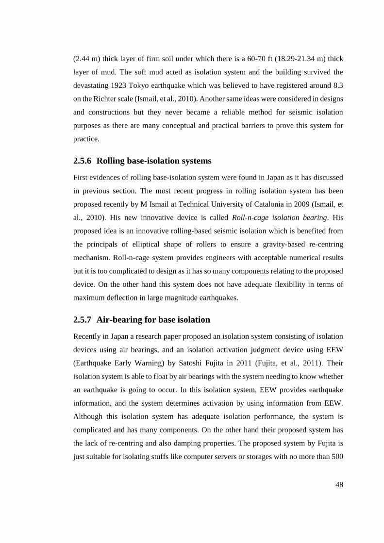
2.5.6 Rolling base-isolation systems
First evidences of rolling base-isolation system were found in Japan as it has discussed
in previous section. The most recent progress in rolling isolation system has been
proposed recently by M Ismail at Technical University of Catalonia in 2009 (Ismail, et
al., 2010). His new innovative device is called Roll-n-cage isolation bearing. His
proposed idea is an innovative rolling-based seismic isolation which is benefited from
the principals of elliptical shape of rollers to ensure a gravity-based re-centring
mechanism. Roll-n-cage system provides engineers with acceptable numerical results
but it is too complicated to design as it has so many components relating to the proposed
device. On the other hand this system does not have adequate flexibility in terms of
maximum deflection in large magnitude earthquakes.
2.5.7 Air-bearing for base isolation
Recently in Japan a research paper proposed an isolation system consisting of isolation
devices using air bearings, and an isolation activation judgment device using EEW
(Earthquake Early Warning) by Satoshi Fujita in 2011 (Fujita, et al., 2011). Their
isolation system is able to float by air bearings with the system needing to know whether
an earthquake is going to occur. In this isolation system, EEW provides earthquake
information, and the system determines activation by using information from EEW.
Although this isolation system has adequate isolation performance, the system is
complicated and has many components. On the other hand their proposed system has
the lack of re-centring and also damping properties. The proposed system by Fujita is
just suitable for isolating stuffs like computer servers or storages with no more than 500

49
kg of weight and further more works are needed to comply with isolating of a structure
like a residential building.
2.5.8 Other isolation systems
There are some other types of isolator, which have been rarely used in isolating
buildings or structures. Rollers, springs, and sleeved piles are some examples of such
isolators. A brief description of those is presented here.
Roller Isolators: Cylindrical rollers and ball races are amongst well-known roller type
isolators. Depends on the structure and material of the roller or ball bearing the
resistance to movement may be sufficient to resist service loads and may generate
damping to some degrees. They have been commonly used for machinery isolation.
Roller bearings are attractive in theory as a simple means of providing flexibility,
however, they have functionality drawbacks in practice. Solid metal ball and roller
bearings made up of steel or alloys usually have the problem of flattening of the contact
surface under time when they are under the weight of huge structures and high
compressive stress which restrict their use. In addition, they are not able to provide either
damping or resistance to service loads; therefore, they should be used in parallel with
other devices such as springs or dampers (Kelly, 2001).
Spring Isolators: There are some devices work based on steel springs which are rarely
used and their most likely application is for machinery isolation. The main drawback
with spring isolators is that they are almost flexible in both the vertical and the lateral
directions (Kelly, 2001). The vertical flexibility in seismic base isolation is not desirable
as it could cause damages in some structural elements. As springs alone can provide just
a little damping and would move disproportionately under service loads, the main
disadvantages of this kind is lack of sufficient damping properties.
Sleeved Piles Isolators: The system comprising piles inside a sleeve can provide
flexibility which allows movement in the structure. Sleeved piles are able to provide
flexibility yet no any degrees of damping (Saiful-Islam, et al., 2011). It is necessary to
use dampers in parallel to the system of sleeved piles for seismic isolation.

50
2.5.9 Advantages and disadvantages of current seismic isolators
As discussed above, some factors may not recognised as the disadvantages of the device
on its own but may be a design disadvantage in the construction projects. As an example,
the high damping rubber bearings could produce primary and secondary (P-∆) moments
which are distributed equally to the top and bottom of the bearing and therefore, these
moments must be designed for in both the foundation and super-structure above the
isolators (Kelly, 2001). For sliding bearing systems, static friction is known as a
disadvantage in general, but for certain construction project, the manufactures of devices
such as the FPS may attempt to produce sliding surfaces reducing this friction as much
as possible. Dampers can be used almost anywhere in a structure to control the
displacements but can add force to the system and cannot be used individually for
isolation. However, depending on the project needs, some characteristics may be found
more important than others.
A lists of significant base isolation projects around the world are given in appendix A.2
BI projects around the world.
2.6 Air-bearing perspective
2.6.1 Applications
Nowadays, the industrial factories benefit from cutting-edge technologies for handling
heavy loads by interposing a fluid layer with low horizontal stiffness between the load
panel and the ground. One of the most well-known technologies is the Air Bearing
system, which produces a thin layer of pressurized air between the load base plane and
the surface of the ground giving an advantage of a near zero friction. The fluid film of
the bearing is achieved by supplying a flow of air through the bearing face and into the
bearing gap. This is typically accomplished through an orifice to provide the flow of air
into the gap (Percision, 2003).

51
Figure 2-6 An air-bearing schematic view
Very similar to an air hockey table, air bearings support even heavy loads on a cushion
of air. Therefore, there is an essential need for a sufficient air pump for practical works.
This kind of air bearings is known as Flat Air Bearing or Rigid Air Bearing (typical flat
air bearing shown in Figure 2-6). Utilising flat air bearings for very heavy loads needs
fairly smooth surfaces as the gap between two surfaces is less than 1 millimetre. The
other kind of air-bearing systems for moving heavy loads is Air Float Bearing. This type
works as similar as hovercrafts. Air float uses a flexible diaphragm beneath the load
support surface. Air is pumped into the diaphragm and passes freely through the
diaphragm holes and into the plenum beneath, raising the platform off the ground.
Figure 2-7 An Air float bearing schematic view (HOVAIR, 2013)
The advantages of air bearing system are identified as follow:
Zero Friction: there is a large difference in the level of friction manifested in an air
bearing system in comparison to the other methods. In air bearing system there is no
difference between static and dynamic coefficient of friction. Friction in air bearings is
a function of air shear from motion.
Silent and smooth operation: rollers or balls create noise at the event of vibration and
become loaded and unloaded whereas an air bearing system does not produce any
notable noise at the time of operation.
Higher damping: Being fluid film bearings, air bearings have a squeeze film damping
effect resulting in higher dynamic stiffness and better controllability.

52
Figure 2-8 Comparison of coefficient of friction for three types of bearing (Newway, 2006)
Air-bearing technology has been utilised in various industries for handling and moving
heavy loads such as diesel engines, machineries, train wagons and also military tanks of
approximately 60 tonnes and higher.
2.6.2 Technical research
The air-bearing solutions have been used for handling heavy weights and also in
precision manufacturing for the past three decades. Nowadays, several companies all
around the world take the advantages of pressurized air for taking heavy loads in
industry and in factories. Companies provide air-bearing solution devices have their
own design procedure and manufacturing. As the choices for design and manufacturing
of a device for a particular purpose of bearing solution could be endless, there are not
organised rules or regulations for the design of air-bearing unit in a specific project.
Beside, manufacturers tend to keep their own research and design unpublished for a
while for competitive purposes. One of the pioneer researchers in this area is John
William Powell who published a book namely “Design of Aerostatic Bearings” in 1970
(Powell, 1970). He introduced basic equations, which are commonly used in the
modelling of the mass flow-rate of gas through an orifice-type restrictor in aerostatic
bearings. In 2004, Renn and Hsiao (Renn & Hsiao, 2004) proposed a CFD simulation
focussing on the mass flow-rate characteristic of gas through orifice, based on using
empirical equations for estimation of controlling coefficients which results in some

53
limitations in application of the method. In 2006, Mukai investigated the dynamic
properties of a manufacturer made air-bearing units (Mukai, 2006). In that report the
effects of shape and geometry of the orifice or nozzle is not presented, whereas the shape
of the nozzle can play a significant role in changing the capacity of air bearing. Another
research by (Wei & Gang, 2010) shows the effect of entrance on load capacity of nozzle.
In their study the density of fluid is assumed as constant which may not lead to accurate
results in turbulence and high Mach numbers.
2.7 Earthquake Early Warning systems
The EEW (Earthquake Early Warning) system can estimate intensity and arrival time of
an earthquake before its principal motion arrives. This is a prevention and warning
system mostly used to control trains, elevators, and medical institution or to warn the
residents of condominium. The principle of the operation and flow of EEW is as follows:
Firstly, seismometers installed near an earthquake focus detect a primary wave, and then
this information is transmitted to the National Meteorological Agency (NMA). Next,
earthquake intensity and estimated time of arrival at a particular place are analysed using
the information of the seismometers. Finally EEW is transmitted from the NMA to
medical institutions, medias, facilities, or residence in order to warn everyone about the
earthquake arrival and thus avoid secondary disaster. Fortunately, EEW systems are
operated and used in many earthquake prone areas of the world. These systems can
provide a few tens of seconds warning prior to damaging ground motions. The amount
of time for early warning depends on the distance from the epicentre of the earthquake.
For example, a study of warning times for the city of San Francisco shows that it is
likely that the city would receive more than 20 sec for the most damaging earthquakes
(Elarms, 2012). Having had the initial alarm, the system could rapidly detect the
initiation of an earthquake, then determine the magnitude and location of the event,
consequently predict the peak ground motion expected in the region around the event,
and at last issue a warning to people in locations that may expect significant ground
motion. The algorithms use data from regional broadband seismic networks. There are
other kinds of similar systems for early warning in other parts of the world like Japan.

54
Therefore, much of the damage and deaths caused by earthquakes will be prevented if
early warning given of a destructive earthquake is used appropriately and effectively.
2.8 Summary
In this chapter Seismic Isolation Systems were investigated from ancient seismic
protection technics to the state-of-the-art practices. It was concluded that not all
proposed techniques were practical. The efficiency of any seismic isolation system
should be measured with respect to the three important aspects: reasonable level of
isolation; adequate level of damping; and re-centring mechanism. Some isolator devices
such as HDRB (High Damping Rubber Bearings) can provide moderate to high level of
damping yet because of strain dependent stiffness properties, they are very complex in
analysis and providing a structure with torsion and P-∆ moments on top and bottom
during an earthquake. Sliding systems, in general, provide a structure with high level of
isolation and moderate damping, but the problem of changeable coefficient of friction
(sometimes leads to sticking) and high level of structural acceleration when using these
types of isolators are yet to resolved. In the lack of a perfect and flawless system,
scientists and researchers have been always looking for overcoming these drawbacks
and difficulties in design. Therefore, there have been ongoing research on the subject of
Seismic Base Isolation either in improving the existing systems or introducing a new
system. The present research introduces a new innovative Seismic Isolation system in
which the requirements of Seismic Base Isolation are satisfied and at the same time, it
overcomes some drawbacks of the current systems.

55
3 New base isolation
system
3.1 Introduction
The new seismic base-isolation system proposed in this study is categorized as Semi-
active systems which triggers with alarms of Earthquake Early Warning (EEW)
systems. The main feature of the new isolation system is taking the advantages of air
bearings. Air bearings provides a thin layer of air between the bottom of device and
contacting surface which enables the unit to handle heavy loads with minimum possible
friction and hence minimum energy. Utilizing air bearings underneath of a structure in
designated points helps in reducing contacts of structure with its base (seismic isolation)
at the time of earthquake and therefore, reducing the damage. This needs an appropriate
design and simulations before applying on real scale structure.
In this chapter, the principals of seismic isolation is explained and the proposed system
is introduced. For better understanding of the performance of the new system, a scaled
structure is designed and tested as a case study. The scaled model is designed based on
a real scale five-story building and the structural characteristics of the scaled model is
based on dimensional analysis and scaling principals. Analytical model of the scaled
structure is then presented based on the assumption of “shear building” and the results
of “dynamic modal analysis” for fixed base and isolated conditions are discussed at the
end.

56
3.2 Seismic base-isolation principals
In general, base isolation techniques follow two basic approaches. Firstly, the isolation
system introduces a layer of low lateral stiffness between a structure and its foundation
underneath. This Isolation layer provides the structure with a natural period which is
much longer than its fixed-base natural period (Chopra, 2007).
𝜔 = √𝑘
𝑚 (3.1)
𝑇 = 2𝜋
𝜔 (3.2)
Here, ω represents the frequency of vibration, m and k denote mass and lateral stiffness
of a structure respectively. The natural period of a structure T, increases by a reduction
of lateral stiffness. As shown by the elastic design spectrum of Figure 3-1, this
lengthening of period can reduce the acceleration and hence the earthquake-induced
forces in a structure, but the deformation is increased. This deformation is concentrated
in the isolation system, however, accompanied by only small deformations in the
structure (Chopra, 2007).
Figure 3-1 Elastic design spectrum, (𝝃 denotes damping) (Chopra, 2007)

57
Secondly, damping is beneficial for reducing the effects of accelerations and forces in a
structure due to an earthquake. A suitable seismic isolation system can produce a level
of acceptable damping.
As a result of reduction in horizontal stiffness of a building at its base in base-isolated
structure and increasing the natural damping, the super-structure will remain undamaged
or slightly damaged after earth shakes. This is schematically presented in Figure 3-2.
Figure 3-2 Behavior of building structure with base-isolation system
An ideal base-isolation condition is when the ground under a structure is moving and
these movements are not transmitted to the structure. If a structure is completely fixed
to ground, it means that stiffness k is infinity; hence, fraction 𝑘 𝑚⁄ has a great value. It
means that 𝜔 (fundamental circular frequency) is very large (see equations 3.1 and 3.2);
therefore fundamental period is near zero. Accordingly, the acceleration induced in the
structure as a result of ground movements is equal to the ground acceleration, and
likewise relative displacement between the structure and ground underneath is zero.
On the other hand, for an ideal seismically-isolated structure, relative horizontal
stiffness is near zero; therefore, fundamental period is infinity; thus, no acceleration
induced in the structure and also relative displacement has some values generally less
than peak ground displacement.
3.2.1 Horizontal isolation
For investigating seismic base-isolation principal, a single degree of freedom structure
is considered (see Figure 3-3); the equation of motion is as follow:

58
𝑚�̈� + 𝑐�̇� + 𝑘𝑢 = −𝑚�̈�𝑔 (3.3)
Where, m is indicating the mass of the structure, c and k representing damping ratio and
stiffness respectively. u is representing the displacement of the structure and ug is the
displacement of the ground, consequently �̈�𝑔 is the ground acceleration during an
excitation. This single story building which is not benefited from any additional
damping system (c equals zero) is isolated form the ground underneath by means of a
set of flexible rubber bearings as it is shown in Figure 3-3.
Figure 3-3 (a) fixed base and (b) isolated structures
A rigid diaphragm of mass mb is added to connect bearings. Each bearing has the
horizontal stiffness of kb/2. The idealized two degrees of freedom (2DOFs) mass-spring
model can be drawn as Figure 3-4. Therefore the governing equation of motion changes
as equations (3.4) (Chopra, 2007).
Figure 3-4 Idealized mass-spring model of 2DOFs structure
[𝑚𝑏 00 𝑚𝑠
] [�̈�𝑏
�̈�𝑠] + [
𝑘𝑏 + 𝑘𝑠 −𝑘𝑠
−𝑘𝑠 𝑘𝑠] [
𝑢𝑏
𝑢𝑠] = [
𝑚𝑏 00 𝑚𝑠
] [10] �̈�𝑔 (3.4𝑎)
[𝑚𝑏 00 𝑚𝑠
] [�̈�𝑏
�̈�𝑠] + [
𝑘𝑏 + 𝑘𝑠 −𝑘𝑠
−𝑘𝑠 𝑘𝑠] [
𝑢𝑏
𝑢𝑠] = [
𝑘𝑏𝑢𝑔
0] (3.4𝑏)

59
Where ub and us are representing displacement of base-mass (𝑚𝑏) and mass of the
structure (𝑚𝑠) respectively. Equation (3.4b) represents the equation of motion with
respect to ground displacement (𝑢𝑔). The total mass of the structure 𝑚 is defined as
follow:
𝑚 = 𝑚𝑏 + 𝑚𝑠 (3.5)
Therefore, nominal frequencies are defined as (3.6).
𝜔𝑏 = √𝑘𝑏
𝑚𝑏 + 𝑚𝑠 , 𝜔𝑠 = √
𝑘𝑠
𝑚𝑠 (3.6)
Expanding the first line of equation of motion (3.4b) gives:
𝑚𝑏�̈�𝑏 + (𝑘𝑏 + 𝑘𝑠)𝑢𝑏 − 𝑘𝑠𝑢𝑠 = 𝑘𝑏𝑢𝑔 (3.7𝑎)
𝑚𝑏�̈�𝑏 + 𝑘𝑏𝑢𝑏 + 𝑘𝑠(𝑢𝑏 − 𝑢𝑠) = 𝑘𝑏𝑢𝑔 (3.7𝑏)
Definition of 𝑥𝑏 and 𝑥𝑠 as relative displacement of base-mass and super-structure
respectively:
𝑥𝑏 = 𝑢𝑏 − 𝑢𝑔 (3.8𝑎)
𝑥𝑠 = 𝑢𝑠 − 𝑢𝑔 (3.8𝑏)
and replacing in equation (3.7b), changes the first line of equation of motion as (3.9)
𝑚𝑏�̈�𝑏 + 𝑘𝑏(𝑥𝑏 + 𝑢𝑔) + 𝑘𝑠(𝑥𝑏 − 𝑥𝑠) = 𝑘𝑏𝑢𝑔 (3.9)
which is simplified to (3.10)
𝑚𝑏�̈�𝑏 + 𝑘𝑏𝑥𝑏 + 𝑘𝑠𝑥𝑏 − 𝑘𝑠𝑥𝑠 = 0 (3.10)
Considering the special case when mb is very small (near zero), equation (3.10) can be
written as (3.11) (Ismail, 2009).
𝑘𝑏𝑥𝑏 + 𝑘𝑠𝑥𝑏 − 𝑘𝑠𝑥𝑠 = 0 (3.11)
Solving for 𝑥𝑏 in terms of 𝑥𝑠 gives

60
𝑥𝑏 =𝑘𝑠
𝑘𝑠 + 𝑘𝑏𝑥𝑠 (3.12)
It is obvious from (3.12) that for a perfect isolated system, where kb is near zero, xs and
and 𝑥𝑏 will have the same value and this means that the structural system acts as a rigid
body.
The second line of matrix equation (3.4b) is expanded as follow:
𝑚𝑠�̈�𝑠 − 𝑘𝑠𝑢𝑏 + 𝑘𝑠𝑢𝑠 = 0 (3.13)
Expanding with respect to equations (3.8):
𝑚𝑠(�̈�𝑠 + �̈�𝑔) − 𝑘𝑠𝑢𝑏 + 𝑘𝑠(𝑥𝑠 + 𝑢𝑔) = 0 (3.14𝑎)
𝑚𝑠�̈�𝑠 + 𝑘𝑠𝑥𝑠 + 𝑘𝑠(𝑢𝑔 − 𝑢𝑏) = −𝑚𝑠�̈�𝑔 (3.14𝑏)
𝑚𝑠�̈�𝑠 + 𝑘𝑠𝑥𝑠 − 𝑘𝑠𝑥𝑏 = −𝑚𝑠�̈�𝑔 (3.14𝑐)
It then follows from substituting (3.12) into (3.14c) that
𝑚𝑠�̈�𝑠 + 𝑘𝑠𝑥𝑠 − 𝑘𝑠𝑘𝑠
𝑘𝑠+𝑘𝑏𝑥𝑠 = −𝑚𝑠�̈�𝑔 (3.15𝑎)
𝑚𝑠�̈�𝑠 + 𝑘𝑠𝑥𝑠(1 − 𝑘𝑠
𝑘𝑠 + 𝑘𝑏) = −𝑚𝑠�̈�𝑔 (3.15𝑏)
Thus, the natural frequency of vibration for isolated structure is defined as (3.16):
𝜔𝑏 = √(1 − 𝑘𝑠
𝑘𝑠 + 𝑘𝑏)
𝑘𝑠
𝑚𝑠 (3.16)
Where √𝑘𝑠
𝑚𝑠 is representing the natural frequency of fixed-base structure. Now the
concepts of period shifting could be understood. The natural period of vibration can be
defined as (3.17):
𝑇𝑏 = 2𝜋
𝜔𝑏 (3.17𝑎)

61
𝑇𝑏 = 2𝜋
√(1 − 𝑘𝑠
𝑘𝑠 + 𝑘𝑏)
𝑘𝑠
𝑚𝑠
(3.17𝑏)
Where, 𝑇𝑏 is the natural period of vibration of the isolated structure. The natural period
of vibration of fixed-base structure is defined by
𝑇𝑠 = 2𝜋
𝜔𝑠=
2𝜋
√𝑘𝑠
𝑚𝑠
(3.18)
Therefore, 𝑇𝑏 can be defined as a multiple of 𝑇𝑠:
𝑇𝑏 = 2𝜋
√(1 − 𝑘𝑠
𝑘𝑠 + 𝑘𝑏)
𝑘𝑠
𝑚𝑠
= 1
√(1 − 𝑘𝑠
𝑘𝑠 + 𝑘𝑏)
2𝜋
√𝑘𝑠
𝑚𝑠
(3.19𝑎)
𝑇𝑏 = 1
√(1 − 𝑘𝑠
𝑘𝑠 + 𝑘𝑏)
𝑇𝑠 = 𝐶𝑝𝑇𝑠 (3.19𝑏)
Where 𝐶𝑝 defined as base isolated natural period coefficient.
For a perfectly fixed-base condition 𝑘𝑏 is infinity so, 𝑇𝑏 equals 𝑇𝑠. When 𝑘𝑏 is much
greater than 𝑘𝑠, then again 𝑇𝑏 approaches the natural period of fixed-base condition. In
a perfectly base-isolated structure, it is assumed that 𝑘𝑏 is near zero, so 𝑇𝑏 is a large
multiple of 𝑇𝑠; it means that the structure will not experience any shocks from ground
underneath and the structure acts as a rigid body (no inter-story drifts). For base-
isolation purposes, designers tend to reduce the ratio of horizontal stiffness of isolators
over stiffness of super-structure, hence, the natural period of the structure will be shifted
to a much greater one in practice. This will benefits the structure in terms of reducing
the acceleration transmitted to the structure and also damage alleviations. Effects of
period shifting in reducing the acceleration experienced by the structure is shown in
Figure 3-5.

62
Figure 3-5 Effects of period shifting in acceleration mitigation
When the fundamental period (also known as natural period of vibration) of a structure
is shifted to a greater one far from the fundamental period of possible shocks, the
structure is highly likely rescued from resonance phenomenon. The frequency in which
resonance happens is also known as resonance frequency. If the structure is driven by a
kind of external dynamic force such as earthquake with a frequency near to its natural
frequency of vibration, resonance happens. In small damping resonance frequency and
natural frequency are approximately the same and equal to a frequency of unforced
vibrations. In practice, resonating vibrations can cause terrific stress and rapid failure of
structural members (Hibbeler, 2002). Thus, it is important to design a structure with a
fundamental frequency far from the frequency of possible shocks. Seismic base isolation
can provide a reasonable gap between the fundamental frequency of isolated structure
and possible earthquake frequencies.
3.2.2 Damping
Damping is beneficial in reducing the effects of earthquakes on a structure. An
appropriate base isolation system is the one which offers reasonable levels of damping.
Considering mass-spring model of Figure 3-4 with damping properties, the effect of
damping on an isolated structure is determined.

63
Figure 3-6 Mass-spring model with damping
Recalling the general equation of motion (3.3) and add damping terms into matrices
form of equation of motion (3.4a), this equation with respect to damping is rewritten as
follow:
[𝑚𝑏 00 𝑚𝑠
] [�̈�𝑏
�̈�𝑠] + [
𝑐𝑏 + 𝑐𝑠 −𝑐𝑠
−𝑐𝑠 𝑐𝑠] [
�̇�𝑏
�̇�𝑠] + [
𝑘𝑏 + 𝑘𝑠 −𝑘𝑠
−𝑘𝑠 𝑘𝑠] [
𝑢𝑏
𝑢𝑠]
= [𝑚𝑏 00 𝑚𝑠
] [10] �̈�𝑔 (3.12)
Where, �̇�𝑏 and �̇�𝑠 corresponds to the velocity of the base-mass and mass of the structure,
respectively. 𝑐𝑏 and 𝑐𝑠 are viscous damping of the isolation system and super structure,
respectively.
At this stage it is necessary to define the nature of isolation system. For example if
sliding isolation system is considered, the following assumptions are applied (De Silva,
2007):
𝑓𝑟 = 𝑘𝑏(𝑢𝑏 − 𝑢𝑏0) 𝑛𝑜𝑛 − 𝑠𝑙𝑖𝑑𝑖𝑛𝑔 𝑝ℎ𝑎𝑠𝑒 (3.13𝑎)
𝑓𝑟 = ±𝜇(𝑚𝑏 + 𝑚𝑠)𝑔 𝑠𝑙𝑖𝑑𝑖𝑛𝑔 𝑝ℎ𝑎𝑠𝑒 (3.13𝑏)
Where,
𝑓𝑟 is frictional force,
𝑘𝑏 is isolation system stiffness,
𝑢𝑏0 is initial elongation of the fictitious spring in the current non-sliding phase,

64
𝜇 is the coefficient of friction,
𝑔 is the acceleration of gravity.
This will add a new term relating to friction force to equation 3.12 as
[𝑚𝑏 00 𝑚𝑠
] [�̈�𝑏
�̈�𝑠] + [
𝑐𝑏 + 𝑐𝑠 −𝑐𝑠
−𝑐𝑠 𝑐𝑠] [
�̇�𝑏
�̇�𝑠] + [
𝑘𝑏 + 𝑘𝑠 −𝑘𝑠
−𝑘𝑠 𝑘𝑠] [
𝑢𝑏
𝑢𝑠] + [
𝑓𝑟0]
= [𝑚𝑏 00 𝑚𝑠
] [10] �̈�𝑔 (3.14)
Applying equation 3.13b in 3.14, the equation of motion of base mass is derived as
follow:
𝑚𝑏�̈�𝑏 + 𝑐𝑏�̇�𝑏 + 𝑘𝑏𝑢𝑏 + 𝜇(𝑚𝑏 + 𝑚𝑠)𝑔. sgn(�̇�𝑏) + 𝑐𝑠�̇�𝑠 + 𝑘𝑠𝑢𝑠 = 𝑚𝑏�̈�𝑔 (3.15)
Basically, the damping properties of a superstructure (𝑐𝑠) is not known explicitly. It can
be constructed by assumptions in modal damping for each mode of vibration. However,
viscous damping of an isolation system is defined as below (Jangid, 1996):
𝑐𝑏 = 2𝜉𝑏𝑀𝜔𝑏 (3.16)
Where,
𝜉𝑏 is damping ratio of the isolation system,
𝜔𝑏 is base isolation frequency.
Equation 3.15 which governs the motion of base mass is non-linear due to the presence
of friction term. The equivalent linear equation obtained by utilizing the time-dependent
equivalent linearization technique (Jangid, 1996) is
𝑚𝑏�̈�𝑏 + 𝑐𝑒�̇�𝑏 + 𝑘𝑏𝑢𝑏 + 𝑐𝑠�̇�𝑠 + 𝑘𝑠𝑢𝑠 = 𝑚𝑏�̈�𝑔 (3.17)
Where,
𝑐𝑒 is equivalent damping and defined as

65
𝑐𝑒 = 𝑐𝑏 +
√2𝜋 𝜇𝑀𝑔
𝜎𝑣�̇�
(3.18)
𝜎𝑣�̇� is the Root-mean-square (RMS) velocity of base mass.
More information about optimum level of damping for an isolation system could be
found in (Jangid, 1996).
Having known the equation of motions (3.12 and 3.14) it is possible to construct the
response spectra with respect to damping for a specific earthquake (Figure 3-1). By
keeping the period of vibration, T, constant and changing the damping ratio, 𝜉; and again
repeat the procedure by keeping the damping ratio, 𝜉, constant and changing the period
of vibration, T, displacement response spectra and pseudo-acceleration response
spectra under a given earthquake are constructed. Acceleration response spectra
correspond to the base shear; the more the base shear the more damage is expected in
the structure at the time of earthquake. These are schematically presented in Figure 3-7
and Figure 3-8.
Figure 3-7 Increase in period of vibration reduces the base shear (Symans, 2004)
Figure 3-7 shows a typical acceleration design response spectra for different damping
levels. Increase in natural period of the structure reduces the acceleration and thus base
shear (force demand) on the structure.
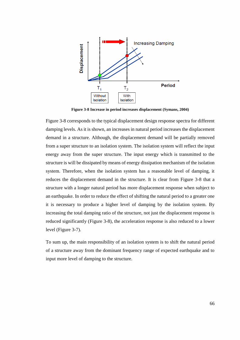
66
Figure 3-8 Increase in period increases displacement (Symans, 2004)
Figure 3-8 corresponds to the typical displacement design response spectra for different
damping levels. As it is shown, an increases in natural period increases the displacement
demand in a structure. Although, the displacement demand will be partially removed
from a super structure to an isolation system. The isolation system will reflect the input
energy away from the super structure. The input energy which is transmitted to the
structure is will be dissipated by means of energy dissipation mechanism of the isolation
system. Therefore, when the isolation system has a reasonable level of damping, it
reduces the displacement demand in the structure. It is clear from Figure 3-8 that a
structure with a longer natural period has more displacement response when subject to
an earthquake. In order to reduce the effect of shifting the natural period to a greater one
it is necessary to produce a higher level of damping by the isolation system. By
increasing the total damping ratio of the structure, not just the displacement response is
reduced significantly (Figure 3-8), the acceleration response is also reduced to a lower
level (Figure 3-7).
To sum up, the main responsibility of an isolation system is to shift the natural period
of a structure away from the dominant frequency range of expected earthquake and to
input more level of damping to the structure.

67
3.3 Innovative isolation system using air bearing
So far there has not been an ideal isolation system to separate the structure from its base
at the time of earthquake with no negative effects. As it was discussed before, the perfect
isolation system is the one which isolates a structure from ground shocks completely
which, however, is almost impossible with respect to the weight of a structure and
uncertainty in the position of the structure after earthquake shocks. The main idea behind
the design of an innovative system in this research is to separate the structure from
horizontal movements of the ground at the time of earthquake with help of air-bearing
solutions. Commercial use of air-bearing technology shows that it is possible to handle
loads up to around 5000 metric tons thanks to the modular design of air caster system
(Aerogo, 2015) (Airfloat, 2015) (Solving, 2015); whereas a typical weigh for building
in total is around 1000 kg per meter square including super imposed load (Monfared, et
al., 2013). Therefore, it is possible to handle a five story building with 100 meter square
area of each floor with existing technology. Indeed, the application of air-bearing
technology is underneath of selected columns with less vertical load to carry, as the
newly proposed isolation system is not going to handle the whole weight of a building.
This innovative isolation system is a combination of air-bearing devices with a re-
centring mechanism which can add some additional damping. The re-centring
mechanism can be provided by one of the existing technologies such as sliding system
in real scale. In this research a simplified method of adding ball bearings and bungee
cords are employed for providing the structure with re-centring mechanism.
The air-bearing devices become active just before the main shocks of earthquake arrive.
And after the main earthquake shocks have gone and the building returns to its original
position the air bearings go off and the building rests. The earthquake early warning
system (EEW) will notify the building sensors if the main shocks seems to be greater
than the designated limit and hence air bearings start to work and isolate the building
from horizontal movements of the ground. Otherwise, for example in reaction to small
shocks or winds the air bearings are inactive. This limit is set in the design prior to
construction and with respect to the importance of the building, seismic performance
constraint and structural conditions (Figure 3-9).
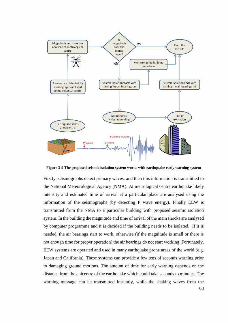
68
Figure 3-9 The proposed seismic isolation system works with earthquake early warning system
Firstly, seismographs detect primary waves, and then this information is transmitted to
the National Meteorological Agency (NMA). At metrological centre earthquake likely
intensity and estimated time of arrival at a particular place are analysed using the
information of the seismographs (by detecting P wave energy). Finally EEW is
transmitted from the NMA to a particular building with proposed seismic isolation
system. In the building the magnitude and time of arrival of the main shocks are analysed
by computer programme and it is decided if the building needs to be isolated. If it is
needed, the air bearings start to work, otherwise (if the magnitude is small or there is
not enough time for proper operation) the air bearings do not start working. Fortunately,
EEW systems are operated and used in many earthquake prone areas of the world (e.g.
Japan and California). These systems can provide a few tens of seconds warning prior
to damaging ground motions. The amount of time for early warning depends on the
distance from the epicentre of the earthquake which could take seconds to minutes. The
warning message can be transmitted instantly, while the shaking waves from the

69
earthquake focus travel through the shallow layers of the Earth at speeds of one to a few
kilometers per second (USGS, 2015). This time is long enough for air bearings to
operate as the existing technology needs a few seconds for full operation (Aerogo,
2015).
3.4 Case study
In order to investigate the new system for seismic isolation, a five-story ordinary
building made up of steel structure with 48 m2 area for each story is considered as a case
study (Figure 3-10). For better understanding of how the new isolation system works, a
1/10th scaled model of case study was designed based on scaling principals and
dimensional analysis. The building was designed based on real sizes and then the
parameters were scaled accordingly.
After determining the dimensions of real scale building, scaling relations in terms of
geometric scaling factor (𝜆) need to be worked out. In this case the scaling factor equals
to 1/10. This scaling factor is chosen with respect to the purpose of the study and
facilities available.

70
Figure 3-10 Schematic view of the case study in real scale
3.4.1 Scaling procedure
As the geometric scaling factor is set to 1/10th the other parameters can be worked out
accordingly. The analysis starts from scaling the mass of each floor. The approximate
mass for each story of a real building in this size is 40 metric tonnes or 40,000 kg. As
the scale factor for length is 0.1 and the scale factor for acceleration and mass density is
considered as 1 (the same material) the dimensional analysis shall be as follow:
λ scale factor in length = 1/10
L real length
l scaled length
M real mass
m scaled mass

71
A real acceleration
a scaled acceleration
D real density
d scaled density
T real time
t scaled time
l/L = λ = 1/10
d/D = 1 (same material)
D ~ ML-3
d/D = ml-3/ML-3 = 1
m/M = L-3/ l-3 = (L/l)-3 = (1/ λ)-3 = 10-3 = 1/1000
thus, mass scaling factor is λ3 or 1/1000.
Which determines 40kg of mass for each story.
The same procedure shall be followed in order to work out the scale factor for time and
the period of the scaled structure.
A ~ LT-2
Therefore,
a/A = lt-2/LT-2 = 1
t-2/T-2 = L/l = 1/ λ = 10
(t/T)-2 = 10
t/T = 10-1/2 = 1/√10 = 1/3.162 = 0.316

72
Same procedure shall be considered in order to work out other parameters scale factor
as follow:
Table 3-1 Scaling relations in terms of geometric scaling factor
Parameter Scaling relations Factor for 1/10th scale
Mass Density 1 1 Acceleration 1 1 Length λ 1/10 Mass λ3 1/1000 Force λ3 1/1000 Time λ1/2 0.316 Frequency λ-1/2 3.162 Stress λ 1/10 Stiffness λ2 1/100
3.5 Scaled model strucutre
Having found the scaled factors for required parameters, it is possible to design and
build the scaled model. With respect to facilities available at the workshop the geometric
scaling factor was chosen as 1/10th which has governed other scale factors. The scaled
model built in the workshop is shown in Figure 3-11. The dimensions of the scaled
model are shown in Figure 3-12. The structural system of the model is moment frame
with rigid connections (structural members can take shear and axial forces as well as
bending moments).

73
Figure 3-11 Scaled model structure built in the workshop
Figure 3-12 Scaled model dimensions (mm)
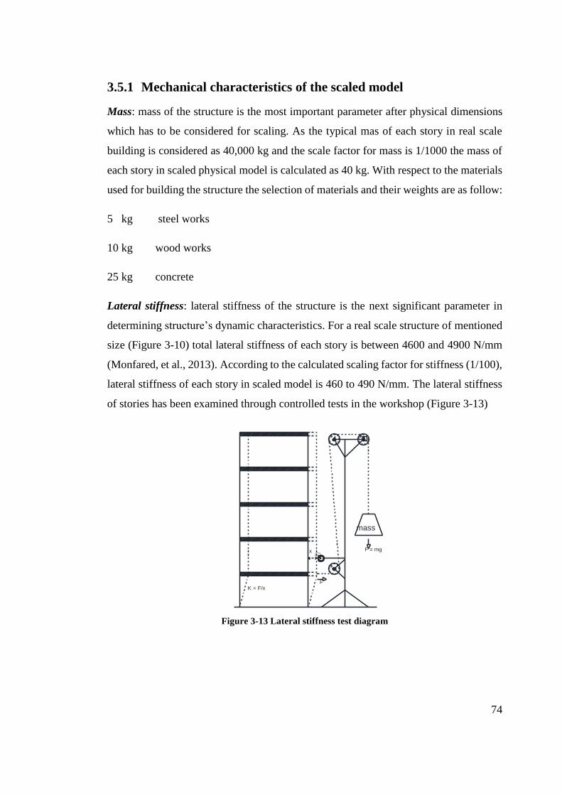
74
3.5.1 Mechanical characteristics of the scaled model
Mass: mass of the structure is the most important parameter after physical dimensions
which has to be considered for scaling. As the typical mas of each story in real scale
building is considered as 40,000 kg and the scale factor for mass is 1/1000 the mass of
each story in scaled physical model is calculated as 40 kg. With respect to the materials
used for building the structure the selection of materials and their weights are as follow:
5 kg steel works
10 kg wood works
25 kg concrete
Lateral stiffness: lateral stiffness of the structure is the next significant parameter in
determining structure’s dynamic characteristics. For a real scale structure of mentioned
size (Figure 3-10) total lateral stiffness of each story is between 4600 and 4900 N/mm
(Monfared, et al., 2013). According to the calculated scaling factor for stiffness (1/100),
lateral stiffness of each story in scaled model is 460 to 490 N/mm. The lateral stiffness
of stories has been examined through controlled tests in the workshop (Figure 3-13)
Figure 3-13 Lateral stiffness test diagram
mass
F = mg
F
x
K = F/x

75
Table 3-2 Results of lateral stiffness test
Force
(N)
Measured
Displacements (mm)
Mean Stiffness
(N/mm)
10x9.81 0.22, 0.21, 0.19, 0.23 461.65
15x9.81 0.30, 0.31, 0.32, 0.30 474.68
20x9.81 0.40, 0.41, 0.42, 0.41 478.53
25x9.81 0.51, 0.54, 0.54, 0.53 462.74
Mean Lateral Stiffness Value (N/mm) 469.4
According to predicted values (460 to 490 N/mm) the mean stiffness value (469.4
N/mm) obtained from experiment is acceptable and used in analytical model.
Fundamental frequency and period: as it was discussed earlier in this chapter, the main
purpose of seismic isolation is to shift the fundamental frequency of vibration to a
smaller one. Therefore, fundamental frequency and corresponding period of vibration
of the structure should be known. The fundamental frequency of vibration of the real
building in this study is between 1.536 and 1.73 Hz and according to the scaling factor
of 1/100.5, the fundamental period of the scaled model is predicted between 4.857 and
5.47 Hz.
Prediction of mechanical characteristics of the scaled model is presented in Table 3-3.
Table 3-3 Prediction of scaled model mechanical characteristics based on scaling factors
Scaling Real Building 1/10 Scaled model
Each Story Mass (kg) 40000 40
Lateral Stiffness (N/mm) 4600 to 4900 460 to 490
Natural Frequency (Hz) 1.536 to 1.73 4.857 to 5.47
Natural Period (s) 0.578 to 0.651 0.183 to 0.206
The dynamic characteristics of the scaled model based on laboratory tests are discussed
in chapter 5.

76
3.5.2 Isolation system for scaled model
The isolation system for the scaled model is designed to resist the vertical loads and to
isolate the structure from its base to a certain levels with capability of re-entering after
shocks due to horizontal movements of base. Air-bearing solution is chosen for the
purpose of isolation of the scaled model and it is used at two points underneath of the
ground floor columns. In order to provide smallest level of contact between the structure
and its base ball bearings are used underneath of other four columns (Figure 3-14)
(Figure 3-15).
Figure 3-14 Isolation system for scaled model

77
Figure 3-15 The air-bearing pallet to be installed underneath of the structure
Figure 3-16 Beneath view of the air-bearing pallet
Figure 3-17 Beneath view of ball-bearing pallet

78
The steel sheet underneath of the isolation system is to provide minimum friction for
ball bearings’ movement as well as provide a smooth surface for air-bearings in
operation (Figure 3-18). The air-bearing device design and specifications are fully
discussed in chapter 4. The specifications of ball bearings used for the isolation system
is given in appendix A.3 Roller bearing specifications.
Figure 3-18 Air bearings installed underneath of the scaled model
Figure 3-19 Air bearings and ball bearings installed underneath of the structure
In order to provide a suitable re-centring mechanism for proposed isolation system,
bungee cords are selected, carefully measured for stiffness and used in the isolation

79
system for scaled model (Figure 3-20). As one of the advantages of the new system,
with changing in the number of bungee cords, different stiffness values are obtained.
Thus, it is possible to define different fundamental periods associated to the isolated
structure.
Figure 3-20 Isolation system for scaled model using bungee cords for re-centring
3.6 Analytical model of the scaled structure
An analytical model of the structure is comprised of a set of structural members includes
structural floors (for mass definition), structural columns (for lateral stiffness definition)
and structural foundation (fixed base or isolated). The analytical structural model of the
scaled structure is shown in Figure 3-21. The analysis of structure is further simplified
by assuming the structure as shear building.
The simplified model of the structure is obtained by assuming that all of the structural
mass is lumped at the floor levels and the floor beams are rigid, whereas, the columns
are axially rigid. These assumptions, along with assuming analysis just for one
horizontal direction at a time, allow for the generation of a model of structure called
shear-type building model. Therefore, displacements at each floor (or lumped mass)

80
level shall be described by one degree-of-freedom alone. Hence, only five degrees of
freedom are needed to describe total displacements of the structure.
A structural system is supposed to have an infinite number of natural frequencies,
however, if the lumped mass approach (shear-type building) is used, the number of
natural frequencies reduced to a finite number corresponding to the number of lumped
mass or degrees of freedom.
Figure 3-21 analytical model of the structure (fixed-base conditions)
3.6.1 Modal analysis
The analytical model is generated to find out the dynamic characteristics of the structure.
Natural frequencies and periods of vibration are of interest in many engineering
applications especially when seismic isolation is considered. Modal Analysis is widely
accepted as a common type of dynamic analysis which is also referred to as an
eigenvalue analysis.
Mode shapes of vibration which arise at the fundamental or natural frequencies are also
discovered in addition to the frequencies. Mode shapes involve dimensionless
representations of the shape that the structure experiences while vibrating at a particular
frequency. This specific frequency is known as the corresponding natural frequency of
the mode shape. These are known as the undamped free vibration response of the
structure due to an initial disturbance (displacement or force) from the equilibrium
position.

81
The solution derives from the general equation of motion (equation 3.3) by zeroing the
damping and applied force terms as (Clough & Penzien, 2003)
𝑀�̈�(𝑡) + 𝐾𝑈(𝑡) = {0} (3.19)
In this equation M and K are mass and stiffness matrices respectively. U(t) defines the
displacement function.
Afterward, it is assumed that each node (lumped mass) is subjected to a sinusoidal
functions of the peak amplitude for that node. If the displacement vector U(t) has the
following form:
𝑈(𝑡) = ∅ sin𝜔𝑡 (3.20)
which gives
�̈�(𝑡) = −𝜔2∅ sin𝜔𝑡 (3.21)
where ∅ is the amplitude of displacement for each node and 𝜔 is the frequency of
vibration, substituting equations 3.20 and 3.21 in equation 3.19 gives the eigenvalue
equation as
𝐾∅ − 𝜔2𝑀∅ = {0} (3.22)
Which has n solutions for n degrees of freedom corresponding to the structure. For a
five-degree-of-freedom structure (the case study in this research) the total number of
eigenvalues or natural frequencies is equal to five.
𝜔𝑖 = natural frequencies (i=1-5)
∅𝑖 =
(
∅1,𝑖
∅2,𝑖
∅3,𝑖
∅4,𝑖
∅5,𝑖)
= natural mode shape of ith frequency
Each eigenvalue or frequency has a corresponding eigenvector or mode shape. Since
each of the eigenvectors cannot be null vectors, the eigenvalues are the roots of the
following equation:
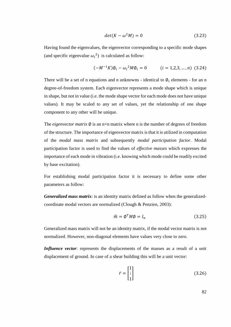
82
𝑑𝑒𝑡(𝐾 − 𝜔2𝑀) = 0 (3.23)
Having found the eigenvalues, the eigenvector corresponding to a specific mode shapes
(and specific eigenvalue 𝜔𝑖2) is calculated as follow:
(−𝑀−1𝐾)∅𝑖 − 𝜔𝑖2𝑀∅𝑖 = 0 (𝑖 = 1,2,3, … , 𝑛) (3.24)
There will be a set of n equations and n unknowns - identical to ∅𝑖 elements - for an n
degree-of-freedom system. Each eigenvector represents a mode shape which is unique
in shape, but not in value (i.e. the mode shape vector for each mode does not have unique
values). It may be scaled to any set of values, yet the relationship of one shape
component to any other will be unique.
The eigenvector matrix ∅ is an n×n matrix where n is the number of degrees of freedom
of the structure. The importance of eigenvector matrix is that it is utilized in computation
of the modal mass matrix and subsequently modal participation factor. Modal
participation factor is used to find the values of effective masses which expresses the
importance of each mode in vibration (i.e. knowing which mode could be readily excited
by base excitation).
For establishing modal participation factor it is necessary to define some other
parameters as follow:
Generalized mass matrix: is an identity matrix defined as follow when the generalized-
coordinate modal vectors are normalized (Clough & Penzien, 2003):
�̂� = ∅𝑇𝑀∅ = 𝐼𝑛 (3.25)
Generalized mass matrix will not be an identity matrix, if the modal vector matrix is not
normalized. However, non-diagonal elements have values very close to zero.
Influence vector: represents the displacements of the masses as a result of a unit
displacement of ground. In case of a shear building this will be a unit vector:
�̅� = [1⋮1] (3.26)
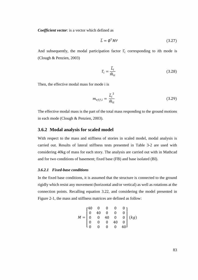
83
Coefficient vector: is a vector which defined as
�̅� = ∅𝑇𝑀�̅� (3.27)
And subsequently, the modal participation factor Γ𝑖 corresponding to ith mode is
(Clough & Penzien, 2003)
Γ𝑖 =�̅�𝑖
�̂�𝑖𝑖 (3.28)
Then, the effective modal mass for mode i is
𝑚𝑒𝑓𝑓,𝑖 = �̅�𝑖
2
�̂�𝑖𝑖 (3.29)
The effective modal mass is the part of the total mass responding to the ground motions
in each mode (Clough & Penzien, 2003).
3.6.2 Modal analysis for scaled model
With respect to the mass and stiffness of stories in scaled model, modal analysis is
carried out. Results of lateral stiffness tests presented in Table 3-2 are used with
considering 40kg of mass for each story. The analysis are carried out with in Mathcad
and for two conditions of basement; fixed base (FB) and base isolated (BI).
3.6.2.1 Fixed-base conditions
In the fixed base conditions, it is assumed that the structure is connected to the ground
rigidly which resist any movement (horizontal and/or vertical) as well as rotations at the
connection points. Recalling equation 3.22, and considering the model presented in
Figure 2-1, the mass and stiffness matrices are defined as follow:
𝑀 =
[ 40 0 0 0 00 40 0 0 00 0 40 0 00 0 0 40 00 0 0 0 40]
(𝑘𝑔)
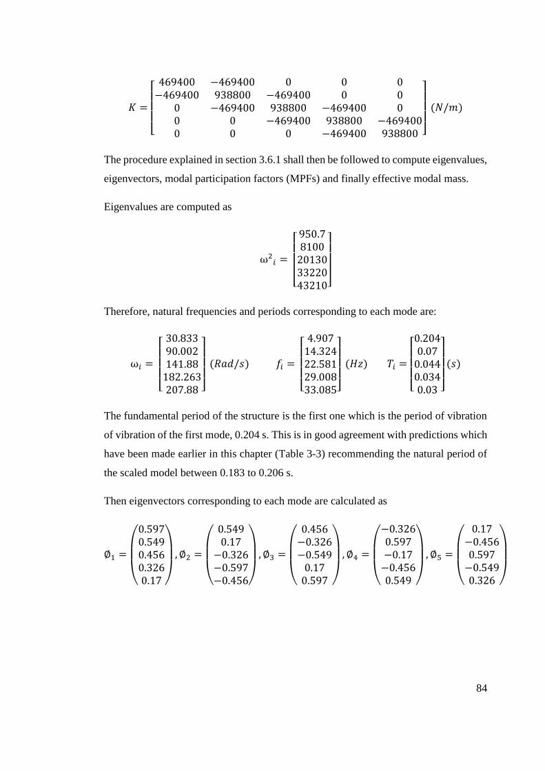
84
𝐾 =
[
469400 −469400 0 0 0−469400 938800 −469400 0 0
0 −469400 938800 −469400 00 0 −469400 938800 −4694000 0 0 −469400 938800 ]
(𝑁/𝑚)
The procedure explained in section 3.6.1 shall then be followed to compute eigenvalues,
eigenvectors, modal participation factors (MPFs) and finally effective modal mass.
Eigenvalues are computed as
ω2𝑖 =
[ 950.78100201303322043210]
Therefore, natural frequencies and periods corresponding to each mode are:
ω𝑖 =
[ 30.83390.002141.88182.263207.88 ]
(𝑅𝑎𝑑/𝑠) 𝑓𝑖 =
[ 4.90714.32422.58129.00833.085]
(𝐻𝑧) 𝑇𝑖 =
[ 0.2040.070.0440.0340.03 ]
(𝑠)
The fundamental period of the structure is the first one which is the period of vibration
of vibration of the first mode, 0.204 s. This is in good agreement with predictions which
have been made earlier in this chapter (Table 3-3) recommending the natural period of
the scaled model between 0.183 to 0.206 s.
Then eigenvectors corresponding to each mode are calculated as
∅1 =
(
0.5970.5490.4560.3260.17 )
, ∅2 =
(
0.5490.17
−0.326−0.597−0.456)
, ∅3 =
(
0.456−0.326−0.5490.170.597 )
, ∅4 =
(
−0.3260.597−0.17−0.4560.549 )
, ∅5 =
(
0.17−0.4560.597
−0.5490.326 )

85
Figure 3-22 Mode shapes corresponding to the scaled structure
Having known the eigenvectors, mode shapes have been drawn (Error! Reference
source not found.). Modal participation factors and effective modal masses are then
computed as follow:
Γ𝑖 =
[ 2.097−0.660.3480.1940.089]
𝑚𝑒𝑓𝑓 =
[ 175.90617.4354.8431.5020.314 ]
It is understood from modal participation factors and effective mass matrix that the
structure is highly likely subject to vibration at first mode at the time of excitation and
mode number five is not likely to be excited. These values are often used in modal
superposition method of dynamic analysis. It should be noted that the sum of the
effective masses must be equal to the total mass of the structure (200 kg). Details of
calculations for this section are given in appendix A.4 Modal analysis (fixed-base
model).

86
3.6.2.2 Isolated conditions
Lateral stiffness of the isolation system will determine the fundamental frequencies and
periods of the isolated structure. Therefore, seismic design codes provides engineers and
designers with provisions which have to be considered in design of seismic isolation
systems for buildings.
Desire period of the isolated structure shall be determined by defining the stiffness of
the isolation system. The more stiff the isolation system, the smaller shift is observed in
the effective isolated period. Therefore, Eurocode 8 recommended the following
expression for identification of the effective isolated period (Eurocode8, 2011):
3𝑇𝑓 ≤ 𝑇𝑒𝑓𝑓 ≤ 3𝑠 (3.30)
Where Teff is the effective fundamental period of the isolated structure and Tf is the
fundamental period of the superstructure assuming in fixed-base condition. The
statement above is recommended for real building and for scaled model it is necessary
to scale the time according to scaling relations in Table 3-1. Therefore, equation 3.30
changes to equation 3.31 for isolated condition as
3𝑇𝑓𝑠𝑐 ≤ 𝑇𝑒𝑓𝑓𝑠𝑐 ≤ 3(0.316)s𝑠 (3.31)
Where, Tfsc and Teffsc represent period of the superstructure in fixed and isolated base
conditions respectively.
The proposed isolation system is able to be set with different values in effective
horizontal stiffness (with changing the number of bungee cords) and subsequently
exhibits different effective periods. With respect to the fixed-base period of 0.204s
(taken from the results of modal analysis in previous section) the limits for effective
isolated period Teffsc are
0.612𝑠 ≤ 𝑇𝑒𝑓𝑓𝑠𝑐 ≤ 0.948𝑠 (3.32)
If the target period of the isolated structure is taken as four times of the fixed-base period
for starting the calculations, Teffsc then is equal to 4(0.204) = 0.816s, which is well lied
in the range recommended by Eurocode 8:

87
0.612 < 0.816 < 0.948s.
A simple relation between effective period and effective stiffness shall determine the
effective stiffness of isolation system for application in analytical model and further in
experimental study.
𝑇𝑒𝑓𝑓 = 2𝜋√𝑀
𝐾𝑒𝑓𝑓 (3.33)
In equation 3.33, 𝑀 represents total mass of the structure and 𝐾𝑒𝑓𝑓 is the effective
horizontal stiffness of the isolation system. It should be noted that the total mass of the
structure in isolated conditions include additional mass base equals to the mass of each
story (here 40kg). Mass base is the lowest level of superstructure to produce an ideal
rigid slab immediately above the isolation system and act as a link between
superstructure and isolation system. Therefore, the mass and stiffness matrices in
isolated conditions have one more row and column to introduce characteristics of
isolation system.
As discussed above the total mass of the structure is 240kg in isolated conditions and as
explained earlier the target effective period is assumed as 0.816s, therefore, according
to equation 3.33, the effective stiffness of the isolation system is calculated as
14229.5N/m.This value is applied in calculations as 14500N/m. Again the procedure
explained in section 3.6.1 is followed for modal analysis of the isolated scaled structure.
𝑀 =
[ 40 0 0 0 0 00 40 0 0 0 00 0 40 0 0 00 0 0 40 0 00 0 0 0 40 00 0 0 0 0 40]
(𝑘𝑔)
𝐾 =
[
469400 −469400 0 0 0 0−469400 938800 −469400 0 0 0
0 −469400 938800 −469400 0 00 0 −469400 938800 −469400 00 0 0 −469400 938800 −4694000 0 0 0 −469400 483900 ]
(𝑁/𝑚)

88
Where, 𝑀 and 𝐾 are mass and stiffness matrices of the scaled model in isolated
conditions. As one additional level is now added to the structure, the number of degrees
of freedom is 6; therefore, 6 number of natural frequencies, periods and mode shapes
are expected.
Natural frequencies and periods corresponding to each mode are:
ω𝑖 =
[
7.59357.075108.75153.399187.712209.294]
(𝑅𝑎𝑑/𝑠) 𝑓𝑖 =
[ 1.2089.08417.30824.41429.87533.31 ]
(𝐻𝑧) 𝑇𝑖 =
[ 0.8270.110.0580.0410.0330.03 ]
(𝑠)
The fundamental period of the structure is now 0.827s which in good agreement with
0.816s of initial assumptions.
∅1 =
(
−0.42−0.418−0.414−0.408−0.4
−0.389)
, ∅2 =
(
−0.552−0.399−0.1350.1660.4210.56 )
, ∅3 =
(
−0.4980.0040.5020.494
−0.012−0.506)
, ∅4 =
(
−0.4070.4090.405
−0.411−0.4030.414 )
, ∅5 =
(
0.288−0.5770.290.286
−0.5770.293 )
, ∅5 =
(
−0.1490.408
−0.5570.558
−0.4090.151 )
Figure 3-23 Mode shapes of isolated scaled structure
Mode shapes are shown in Figure 3-23. Modal participation factors and effective modal
masses are then computed as follow:

89
Γ𝑖 =
[ −2.4490.062
−0.0150.00640.0030.0013]
𝑚𝑒𝑓𝑓 =
[ 239.830.1550.00960.00160.00030.0000]
It is concluded from modal participation factors and effective mass matrix that the
structure is highly likely excited at the first mode of vibration. Full computation details
are presented in A.5 Modal analysis (base isolated).
3.6.2.3 Discussion
Comparing the results from modal analysis of the structure (scaled model) once again
reveals the importance of period shifting in the response analysis of the structures. It is
understood from modal participation factors in two conditions (fixed base and isolated)
that the effect of second, third, fourth and fifth modes of vibration are negligible thanks
to the isolation system. The most effective mode in isolated structure is the first mode
which is shifted far beyond the likely period of devastating shocks.
In addition, comparison of the mode shapes of the structure in fixed-base and isolated
conditions, illustrates how relative story drifts are reduced in isolated structure.
According to the results from analysis of the scaled structure, the first mode of vibration
is the most significant one (i.e. structural vibration in this mode is highly likely). There
are great reductions in the values corresponding to story drifts in fixed base condition
compared to isolated (Table 3-4).
Table 3-4 Story drifts
Stories drifts (non-dimensional)
fixed base isolated
5th - 4th 0.048 0.002
4th - 3rd 0.093 0.004
3rd - 2nd 0.13 0.006
2nd - 1st 0.156 0.008
1st - base 0.17 0.011
base - zero - 0.389

90
The smaller the inter-story drifts, the less damage is expected in the structure after
earthquake shocks.
3.7 Conclusion
In this chapter the philosophy of seismic base isolation was discussed and a case study
was introduced along with the principals of scaling for a scaled structure. The analytical
model of the case study was presented and the dynamic properties of the structure were
investigated. It was shown how the appropriate base isolation system can reduce the
effects of dynamic loads on the structure in theory, with shifting the period of the
structure to a greater one and reducing story drifts as the cause of damage. The results
will be further discussed and compared with experimental tests results in chapter five.
As the main element of the new isolation system is air bearings, chapter four presents
the design and development of air-bearing devices through numerical simulations and
laboratory tests.

91
4 Air-bearing device design
and development
4.1 Introduction
The air-bearing units used for the purpose of this study are categorised as flat air
bearing made of Aluminium materials. With respect to the size of the structure (5-story
scaled building model), available materials in the market and capabilities of the CNC
machine in the workshop, a 3D model for the device was generated in a CAD software
and analysed through a numerical modelling then the results have been validated via
laboratory tests and analytical study. The geometry and number of nozzles have been
further optimized to achieve best performance for air bearing devices.
4.2 Air bearing design
The air bearing designed for this study is a flat air bearing in which the nozzle outlet
blow a vertical jet of air directly to the surface underneath and unlike the cushion type
bearings there is no rubber made cushion below the device to maintain the air volume.
Flat bearings maintain a finite separation between mechanical components by means of
the pressurized flow of air through the gap between two surfaces. A well-known
example of this kind is an air hockey table, where a puck is floated above the table
surface by an array of vertical jets of air (Hendriks, 2001). Using flat air bearings there
is no contact between “moving parts” and thus no friction and no wear on surfaces.

92
The design of the bearing for this study consists of the design of the nozzle shape for
flat type air bearing. The size of the chamber of the bearing is restricted by the maximum
of 200mm and 50mm for exterior diameter and height respectively. These dimensions
are all determined by the space restrictions at the base of the structure. According to
these constraints and the capabilities of the CNC machine in the workshop, the geometry
of the air-bearing device is determined as shown in Figure 4-1 and Figure 4-2.
Figure 4-1 Air-bearing device chamber (dimensions in mm)
The seal of the bearing is attached to the chamber through the designated screw holes
on the wall of the chamber.
Figure 4-2 Air-bearing seal with nozzles (dimensions in mm)

93
The changeable seal gives the opportunity of testing different nozzle shapes and
numbers. Having known the feasible size and geometry for the bearings, it is possible
to model it in a CAD software and analyse the fluid flow with respect to the maximum
pressure available at the workshop. Simulations are to determine the optimum geometry
for nozzles and further optimisation of the number of nozzles. The primary shape of
nozzle for this type of air bearing consists of an orifice with a cylindrical pocket. The
shape considered for initial simulation is a conical shape shown in Figure 4-3.
Figure 4-3 Nozzle geometry used in air-bearing design
The flow enters the nozzle from 2mm diameter side and exits from 6mm diameter. In
fact, the inlet of the nozzle is designed to have the smaller diameter than its outlet. The
flow that enters the nozzle reaches Mach velocity rapidly due to high pressure
differences between inlet and outlet. As the flow becomes supersonic, the nozzle should
have divergent shape to maintain the high velocity otherwise, the flow velocity will drop
to subsonic area.

94
Figure 4-4 The effects of divergence in nozzle shape on flow parameters (Beychok, 2010)
The higher velocity is desire as it produces higher momentum.
In order to gain an insight into what happens to the flow inside the chamber and nozzle,
it is necessary to create a computer simulation with respect to the geometry constraints
and boundary conditions. The simulation also provides valuable information about the
fluid characteristics such as pressure, velocity and consequently mass flow rate. Mass
flow rate can be used to validate the total momentum force generated in nozzle. Next
section will discuss the simulation method in light of the governing equations of fluid
flow.
4.3 Simulation methods
4.3.1 Governing equations
The governing equations of the fluid flow could be described by the problems of
continuum mechanics. In continuum motion the governing equation are as follow (Aris,
1989):
𝑑
𝑑𝑡∫ 𝜌∅(𝐱, 𝑡)𝑑𝑉 =
𝜕
𝜕𝑡∫ 𝜌∅𝑑𝑉𝑉𝑀(𝑡)
+ ∮ 𝑑𝐒𝜕𝑉𝑀(𝑡)𝑉𝑀(𝑡)
. (𝜌∅𝐔), (4.1)

95
In equation 4.1, U is the velocity vector and dS is the outward pointing unit vector
normal to 𝜕𝑉𝑀(𝑡). The rate of change of ∅ in 𝑉𝑀 can be written regarding its volume
and surface sources:
𝜕
𝜕𝑡∫ 𝜌∅𝑑𝑉𝑉𝑀(𝑡)
+ ∮ 𝑑𝐒𝜕𝑉𝑀(𝑡)
. (𝜌∅𝐔) = ∫ 𝑄𝑉(∅)𝑑𝑉 + ∮ 𝑑𝐒. 𝐐𝑆(∅), (4.2)𝜕𝑉𝑀(𝑡)𝑉𝑀(𝑡)
The differential form of the above is:
𝜕𝜌∅
𝜕𝑡+ ∇. (𝜌∅𝐔) = 𝑄𝑉(∅) + ∇. 𝐐𝑆(∅). (4.3)
Equation 4.3 is a governing equation for all continuum mechanics problems in general
(Aris, 1989). The equation is transformed to different conservation equations by
changing parameter ∅ .
The conservation laws valid for any continuum are as follow:
- Conservation of mass (∅ = 1)
𝜕𝜌
𝜕𝑡+ ∇. (𝜌𝐔) = 0 (4.4)
- Conservation of linear momentum (∅ = U)
𝜕𝜌𝐔
𝜕𝑡+ ∇. (𝜌𝐔𝐔) = 𝜌𝐠 + ∇. 𝜎 (4.5)
- Conservation of energy (∅ = e)
𝜕𝜌𝑒
𝜕𝑡+ ∇. (𝜌𝑒𝐔) = 𝜌𝐠. 𝐔 + ∇. (𝜎. 𝐔) − ∇. 𝐪 + 𝜌𝑄. (4.6)
Where
- 𝜌 is the density,
- U is the velocity vector,
- 𝜎 is the stress tensor,
- 𝑒 is the total specific energy,
- 𝑄 is the volume energy source.

96
The system is still indeterminate as the number of unknown quantities is larger than the
number of equations. There is a need to introduce additional conservative relations to
increase the number of equations and close the system.
Considering the fluid as a Newtonian fluid, the following set of equations can be used
(Jasak, 1996):
Defining the internal energy as a function of pressure P and temperature T:
𝑢 = 𝑢(𝑃, 𝑇). (4.6)
The total energy 𝑒 can be defined as the sum of the kinetic energy 𝑒𝑘 and internal
energy:
𝑒 = 𝑒𝑘 + 𝑢(𝑃, 𝑇) =1
2 𝐔. 𝐔 + 𝑢(𝑃, 𝑇) (4.7)
The equation of state:
𝜌 = 𝜌(𝑃, 𝑇), (4.8)
The Fourier’s law of heat conduction:
𝐪 = −𝜆∇𝑇, (4.9)
Where
- 𝐪 is the heat flux,
- 𝜆 is the transport coefficient
Generalised form of the Newton’s law of viscosity (Jasak, 1996):
𝜎 = −(𝑃 +2
3𝜇∇. 𝐔) 𝐈 + 𝜇[∇𝐔 + (∇𝐔)𝑇]. (4.10)
Where
- 𝜇 is viscosity
- 𝐈 is the unit tensor
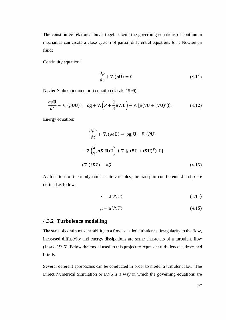
97
The constitutive relations above, together with the governing equations of continuum
mechanics can create a close system of partial differential equations for a Newtonian
fluid:
Continuity equation:
𝜕𝜌
𝜕𝑡+ ∇. (𝜌𝐔) = 0 (4.11)
Navier-Stokes (momentum) equation (Jasak, 1996):
𝜕𝜌𝐔
𝜕𝑡+ ∇. (𝜌𝐔𝐔) = 𝜌𝐠 + ∇. (𝑃 +
2
3𝜇∇. 𝐔) + ∇. [𝜇(∇𝐔 + (∇𝐔)𝑇)], (4.12)
Energy equation:
𝜕𝜌𝑒
𝜕𝑡+ ∇. (𝜌𝑒𝐔) = 𝜌𝐠. 𝐔 + ∇. (𝑃𝐔)
− ∇. (2
3𝜇(∇.𝐔)𝐔) + ∇. [𝜇(∇𝐔 + (∇𝐔)𝑇). 𝐔]
+∇. (𝜆∇𝑇) + 𝜌𝑄. (4.13)
As functions of thermodynamics state variables, the transport coefficients 𝜆 and 𝜇 are
defined as follow:
𝜆 = 𝜆(𝑃, 𝑇), (4.14)
𝜇 = 𝜇(𝑃, 𝑇). (4.15)
4.3.2 Turbulence modelling
The state of continuous instability in a flow is called turbulence. Irregularity in the flow,
increased diffusivity and energy dissipations are some characters of a turbulent flow
(Jasak, 1996). Below the model used in this project to represent turbulence is described
briefly.
Several deferent approaches can be conducted in order to model a turbulent flow. The
Direct Numerical Simulation or DNS is a way in which the governing equations are

98
numerically integrated (Eswaran & Pope, 1988). The Large Eddy Simulation (LES) is
another way in which a spatial filter is applied in order to separate different length scales
which was first introduced by (Deardorff, 1970). Both two ways are among the pioneers
in fluid turbulence numerical analysis yet demanding high computer specifications and
rendering time.
An alternative approach is separation of the local value of the variable into the mean
value and the fluctuation around the mean. In this case the characteristics of turbulent
flow governs the selection of averaging method.
Reynolds averaging technique: One of the popular techniques is Reynolds averaging
technique in which all flow parameters are presented as mean value plus a fluctuation
value as follow:
∅(𝐱, 𝑡) = ∅̅(𝐱, 𝑡) + ∅′(𝐱, 𝑡), (4.18)
where ∅′(𝐱, 𝑡) is the fluctuation about the mean value and the mean value is defined as
below:
�̅�(𝐱, 𝑡) = limN→∞
1
𝑁∑𝜙𝑖(𝐱, 𝑡)
𝑁
𝑖=1
, (4.19)
In this equation N is the number of identically performed experiments.
The following form of the averaged will be obtained if the above procedure is applied
to the compressible1 Navier-Stokes equation:
𝜕
𝜕𝑡(𝜌�̅�) + ∇. (𝜌�̅��̅�) = 𝐠 − ∇�̅� + ∇. (𝜈∇�̅�) + 𝐔′𝐔′̅̅ ̅̅ ̅̅ . (4.20)
The term 𝐔′𝐔′̅̅ ̅̅ ̅̅ is called the Reynolds stress tensor. The Reynolds stress represent
effects of the turbulence and has to be modelled to close the system of equations
(Ramezanpour, 2009).
1 It should be noted that this analysis is based on compressible flow principals.
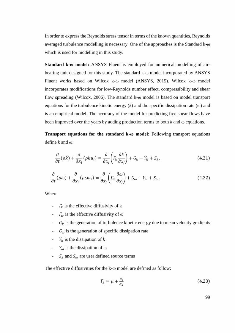
99
In order to express the Reynolds stress tensor in terms of the known quantities, Reynolds
averaged turbulence modelling is necessary. One of the approaches is the Standard k-ω
which is used for modelling in this study.
Standard k-ω model: ANSYS Fluent is employed for numerical modelling of air-
bearing unit designed for this study. The standard k-ω model incorporated by ANSYS
Fluent works based on Wilcox k-ω model (ANSYS, 2015). Wilcox k-ω model
incorporates modifications for low-Reynolds number effect, compressibility and shear
flow spreading (Wilcox, 2006). The standard k-ω model is based on model transport
equations for the turbulence kinetic energy (k) and the specific dissipation rate (ω) and
is an empirical model. The accuracy of the model for predicting free shear flows have
been improved over the years by adding production terms to both k and ω equations.
Transport equations for the standard k-ω model: Following transport equations
define k and ω:
𝜕
𝜕𝑡(𝜌𝑘) +
𝜕
𝜕𝑥𝑖
(𝜌𝑘𝑢𝑖) =𝜕
𝜕𝑥𝑗(𝛤𝑘
𝜕𝑘
𝜕𝑥𝑗) + 𝐺𝑘 − 𝑌𝑘 + 𝑆𝑘, (4.21)
𝜕
𝜕𝑡(𝜌𝜔) +
𝜕
𝜕𝑥𝑖
(𝜌𝜔𝑢𝑖) =𝜕
𝜕𝑥𝑗(𝛤𝜔
𝜕𝜔
𝜕𝑥𝑗) + 𝐺𝜔 − 𝑌𝜔 + 𝑆𝜔 . (4.22)
Where
- 𝛤𝑘 is the effective diffusivity of k
- 𝛤𝜔 is the effective diffusivity of ω
- 𝐺𝑘 is the generation of turbulence kinetic energy due to mean velocity gradients
- 𝐺𝜔 is the generation of specific dissipation rate
- 𝑌𝑘 is the dissipation of k
- 𝑌𝜔 is the dissipation of ω
- 𝑆𝑘 and 𝑆𝜔 are user defined source terms
The effective diffusivities for the k-ω model are defined as follow:
𝛤𝑘 = 𝜇 +𝜇𝑡
𝜎𝑘 (4.23)

100
𝛤𝜔 = 𝜇 +𝜇𝑡
𝜎𝜔 (4.24)
In these equations:
- 𝜇𝑡 is the turbulent viscosity
- 𝜎𝑘 is the turbulent Prandtl number for k
- 𝜎𝜔 is the turbulent Prandtl number for ω
The relation between k and ω is defined as follow:
𝜇𝑡 = 𝛼∗𝜌𝑘
𝜔 (4.25)
Note that in the high-Reynolds number form of the k-ω model, 𝛼∗ = 𝛼∞∗ = 1.
4.4 Numerical solutions
As there is no analytical solution for partial differential equations governing fluid flow
problems and on the other hand, experimental study is costly and time taking for high
number of design variables, the best option to analyse and finalise the air-bearing design
is using numerical methods for the solution of mathematically defined fluid flow
governing equations. CFD (Computational Fluid Dynamics) analysis is employed for
solving the problem of fluid flows in this study in order to determine the optimised
geometry of the nozzles.
4.4.1 Geometry
CFD analysis starts with generating the geometry of the model. It should be noted that,
all geometry components are parametric in this model which enables the user to change
them for desire dimensions. The general geometry of the air-bearing unit used in this
study is shown in Figure 4-5.

101
Figure 4-5 CFD model volume (dimensions in mm)
The geometry of CFD model is a cylinder shape volume with diameter of 130 mm and
height of 20 mm. The inlet has the length of 20mm and diameter of 10 mm. The outlet
is a nozzle to the centre of bottom plate Figure 4-6.
The thickness of bottom plate is 6mm and the material of the device is Aluminium. The
air-bearing unit can lift up with producing a thin layer of air flow underneath of the
bottom. The air pressure on the inlet of the unit is set to 5bars (gauge). The CFD model
for this analysis is responsive when applying changes in inlet and outlet boundaries.
Figure 4-6 Geometry of flow domain
4.4.2 Discretisation
Discretisation is known as the process of transferring the continuous equations or
function into separate complements. This is the primary step toward making the system
of equations or model suitable for numerical analysis. Discretisation consists of three
key steps:

102
Equations discretisation: The partial differential equations of governing equations are
expressed in algebraic form, in terms of discrete quantities defined at each cell in the
domain. Therefore, equation 4.3 becomes
𝑎𝑝∅𝑝𝑡+∆𝑡 = ∑ 𝑎𝑛𝑏∅𝑛𝑏
𝑡+∆𝑡 + 𝑆𝐾
𝑛𝑏
𝑓=1
(4.26)
Where 𝑎𝑝 and 𝑎𝑛𝑏 represent the cell centre and neighbouring cell coefficient
respectively. The cell centre coefficient is calculated as follow (Brennan, 2001):
𝑎𝑝 = ∑ 𝑎𝑛𝑏 − 𝑆𝐿
𝑛𝑏
𝑓=1
(4.27)
In equations 4.26 and 4.27, 𝑆𝐾 and 𝑆𝐿 are dimensionless source terms in integration.
Temporal discretisation: Time domain is divided into finite number of time intervals
or steps in transient problems.
Domain discretisation: The problem space or the domain of the model is divided into
finite number of volumes or regions, known as control volume or mesh.
The numerical solution in this study is based on finite volume method in which the
integral form of the governing equations on each control volume or cell is considered.
Therefore, the flow domain is subdivided into tetrahedral cells where governing
equations are solved subsequently. Control volume or cells fill the whole domain
volume and do not overlap. With respect to the geometry of the domain and the solution
method, the discretisation can be carried out in two different methods:
Structured grid: The cells (meshes) have regular connectivity made it more effective
for simple geometries. The suitable mesh choices are quadrilateral in two dimensional
domains and hexahedra in three dimensional domains. As the neighbourhood
relationships between cells are defined by storage arrangement, this model is highly
space and time efficient with higher resolution than unstructured grid (Castillo, 1991).
Unstructured grid: The best option when irregular geometries for domain is governing
the problem conditions. According to cells irregular connectivity, unstructured grids can

103
be arranged in any convenient manner which provides more freedom in refinement in
specific regions. In comparison to structured meshes, this model can be highly space
and time inefficient as it calls for explicit storage of neighbourhood relationships. These
kind of grids normally hire triangle shapes in two dimensional and tetrahedral in three
dimensional domains (Mavriplis, 1996).
4.4.3 Mesh generation
For this geometry, approximately, 3 million tetrahedral unstructured cells are generated
with prism layer mesh at the boundaries to capture velocity gradients near the walls1.
There is higher mesh density inside the nozzle in order to capture shock waves and
expansion fans (Figure 4-7).
Figure 4-7 Mesh generation by ANSYS Mesh
4.4.4 Numerical setting
For this research, density base solver has been employed with implicit steady state
condition for time frame. In order to reduce the errors, high order of discretisation
schemes has been used. For momentum equations, third order MUSCL scheme has been
adopted and for rest of the parameters second order upwind method has been
implemented. To avoid instabilities in the solution domain, Courant number (CFL) was
set to be below one. As the simulations are carried out for compressible flow, therefore,
the air has been considered as ideal gas. As explained before 𝑘 − 𝜔 turbulent model was
selected to solve Reynolds stress model.
1 This is due to capture boundary layer effect near the wall.

104
4.4.4.1 Boundary conditions
The partial differential equations governing the problem needs boundary conditions in
order to close the system of equations. The solver used for this study is FLUENT
commercial package. The set of boundary conditions implemented are as below:
The inlet boundary condition is defined as “pressure inlet” of 5bar gauge. The flow
inside the chamber and inside the nozzle is solved for different pressure ratios. The inlet
pressure to the chamber is known; on the other hand the velocity and mass flow rate are
unknown. The relationship between variables in the case of compressible flow is as
follow:
𝑝𝑡 = 𝑝𝑠(1 +𝛾 − 1
2𝑀2)
𝛾𝛾−1 (4.28)
Where,
𝑝𝑡 is total pressure,
𝑝𝑠 is the static pressure,
𝛾 is the specific heat ratio and
𝑀 is Mach number defined as below:
𝑀 =𝑢
√𝛾𝑅𝑇𝑠
(4.29)
In the above equation, 𝑢 represents the velocity, 𝑇𝑠 is the static temperature and 𝑅
denotes the gas constant. The static temperature relationship with total temperature is
described as
𝑇𝑡
𝑇𝑠= 1 +
𝛾 − 1
2𝑀2 (4.30)
The outlet boundary condition is defined as “pressure outlet” which is atmospheric
conditions pressure of 1.013bar (zero gauge).

105
The solid wall boundary condition is utilised for solid regions, with no slip conditions.
In order to take into account the effect of viscosity of the flow on the solid walls, the
wall boundary conditions are imposed the shear stress for laminar flows, which are
calculated (based on the velocity gradient at the wall) as below:
𝜏𝑤 = 𝜇𝜕𝑢
𝜕𝑛 (4.31)
Where,
𝜏𝑤 is shear stress at the wall and
𝜇 is the coefficient of friction.
4.4.5 Numerical results
CFD model in this study is a parametric model with capability of applying changes in
all geometry parameters.
The CFD was applied for three different nozzle geometries (Table 4-1) and a gap height
of 1 mm between the bottom of the air-bearing device and the flat surface. In all three
cases the inlet diameter was set to 2mm, however, the simulation was performed for
three different outlet diameters.
Table 4-1 Simulation cases definition
Simulation case
Inlet diameter (mm)
Outlet diameter (mm)
2-3 2 3
2-6 2 6
2-12 2 12
4.4.5.1 Mach contours analysis
In order to determine the optimum slope for conical nozzle, the effect of velocity in
nozzle should be considered. Figure 4-8, Figure 4-9 and Figure 4-10 show the contours
of Mach number in the cross-sectional area of nozzle and gap for three different nozzles.
Mach number is the ratio of actual velocity over the velocity of sound which is helpful

106
for investigating the velocity of compressible flow in a specific field and observation of
shock waves.
In a flow field, Stagnation point is a point with zero local velocity (Clancy, 1975).
According to Bernoulli equation, pressure and velocity have inverse relationship; the
pressure is at its maximum level when the velocity is minimum. Therefore, in fluid flow
where the velocity is zero or near zero (stagnation point), the static pressure is
maximum. This pressure is called Stagnation pressure. With reference to Figure 4-8 to
Figure 4-10, the largest area of stagnation pressure exists in the case of nozzle with 2
mm inlet and 6 mm outlet (Figure 4-9). The stagnation area creates a cushion of air that
the air bearing stands on it. Therefore, it can produce more uplift pressure underneath
of the bottom plate of air-bearing unit.
Figure 4-8 Output results for Mach number (nozzle 2-3 side view)
Figure 4-9 Output results for Mach number (nozzle 2-6 side view)
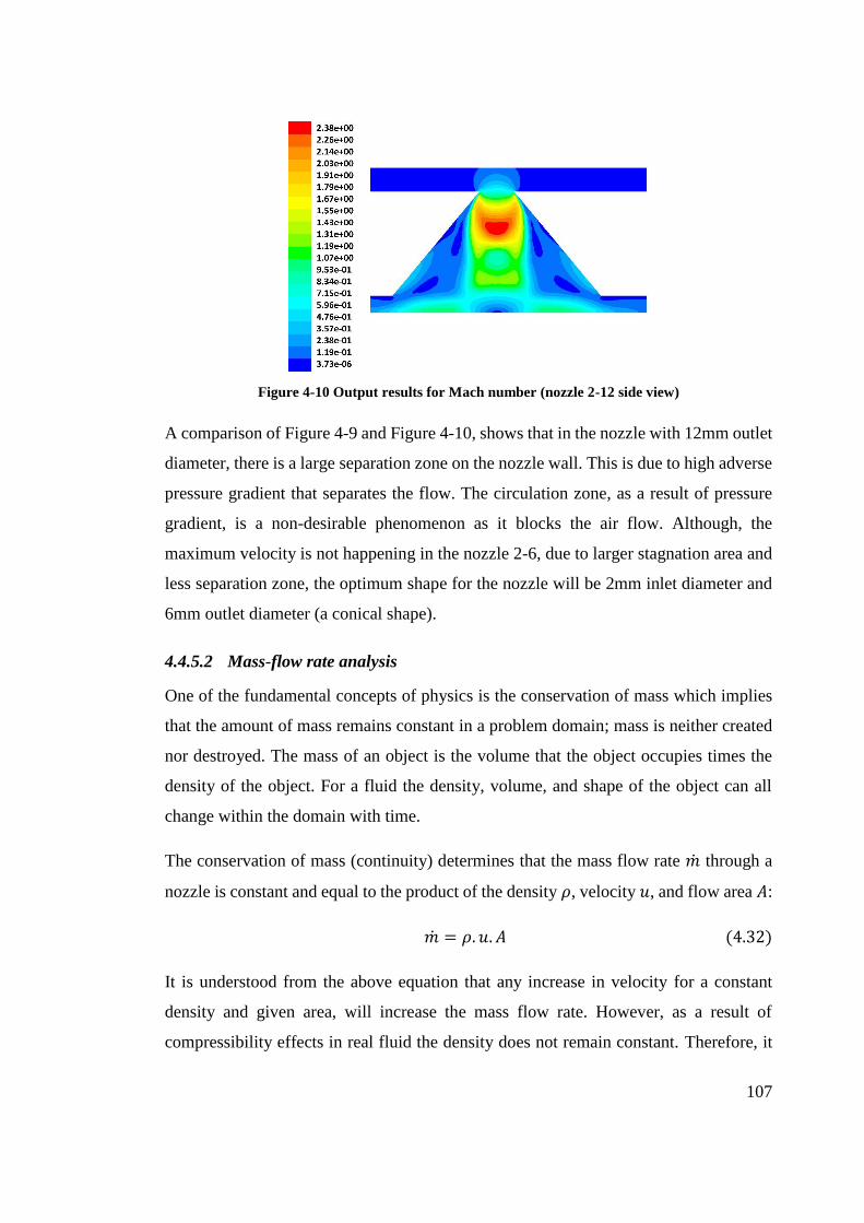
107
Figure 4-10 Output results for Mach number (nozzle 2-12 side view)
A comparison of Figure 4-9 and Figure 4-10, shows that in the nozzle with 12mm outlet
diameter, there is a large separation zone on the nozzle wall. This is due to high adverse
pressure gradient that separates the flow. The circulation zone, as a result of pressure
gradient, is a non-desirable phenomenon as it blocks the air flow. Although, the
maximum velocity is not happening in the nozzle 2-6, due to larger stagnation area and
less separation zone, the optimum shape for the nozzle will be 2mm inlet diameter and
6mm outlet diameter (a conical shape).
4.4.5.2 Mass-flow rate analysis
One of the fundamental concepts of physics is the conservation of mass which implies
that the amount of mass remains constant in a problem domain; mass is neither created
nor destroyed. The mass of an object is the volume that the object occupies times the
density of the object. For a fluid the density, volume, and shape of the object can all
change within the domain with time.
The conservation of mass (continuity) determines that the mass flow rate �̇� through a
nozzle is constant and equal to the product of the density 𝜌, velocity 𝑢, and flow area 𝐴:
�̇� = 𝜌. 𝑢. 𝐴 (4.32)
It is understood from the above equation that any increase in velocity for a constant
density and given area, will increase the mass flow rate. However, as a result of
compressibility effects in real fluid the density does not remain constant. Therefore, it

108
is essential to take into account the effect of change in density in higher velocities.
Recalling equation 4.29 and substitute for velocity in equation 4.32, the compressible
form of the mass flow rate equation is derived as
�̇� = 𝜌. 𝐴. 𝑀√𝛾𝑅𝑇 (4.33)
Equation of state determines density as follow:
𝜌 =𝑝
𝑅𝑇 (4.34)
As the flow is assumed to maintain the constant value of entropy, isentropic1 flow
governing equations are applied:
𝑝 = 𝑝𝑡 (𝑇
𝑇𝑡)
𝛾𝛾−1
(4.35)
𝑇 =𝑇𝑡
1 +12
(𝛾 − 1)𝑀2 (4.36)
Where, 𝑝𝑡 and 𝑇𝑡 are total pressure and total temperature respectively.
By collecting terms and substituting 4.34, 4.35 and 4.36 into 4.33 the equation for mass
flow rate is derived as
�̇� =𝐴. 𝑝𝑡
√𝑇𝑡
. √𝛾
𝑅 .𝑀(1 +
𝛾 − 1
2 .𝑀2)
− 𝛾+1
2(𝛾−1) (4.37)
The maximum flow rate occurs when the Mach number is equal to one (Bailey, 1961).
This phenomenon is known as choking of the flow (Bernstein, et al., 1967). If 𝑀 = 1
is replaced in equation 4.37, the value of the choked mass flow rate is determined as
�̇� =𝐴. 𝑝𝑡
√𝑇𝑡
. √𝛾
𝑅 . (
𝛾 + 1
2 )
− 𝛾+1
2(𝛾−1) (4.38)
1 Isentropic flow occurs, if the changes in flow variables are small and gradual, e.g. the ideal gas flow
through a nozzle.
109
Figure 4-11 Mass flow rate through ta nozzle at different pressure ratios (Tiwari, et al., 2013)
The mass flow rates are calculated at cross section area where 𝑀 = 1 using equation
4.38 for three case studies. The results are presented in Table 4-2.
Table 4-2 Mass flow rate calculated for three different cases
Nozzle inlet diameter (mm)
Nozzle outlet diameter (mm)
Outlet/Inlet
flow rate (kg/s)
2 3 1.5 0.0313
2 6 3 0.0388
2 12 6 0.0327
The higher mass flow rates provides more momentum force. It is understood from table
above, that nozzle 2-6 demonstrates the highest mass flow rate through the nozzle. These
values will be used further on for validation of the numerical modelling.
4.5 Experimental study
Laboratory tests were conducted to validate the results from numerical study on air-
bearing unit in terms of choosing the optimum option for nozzle shape (Figure 4-12).
Three different types of nozzle (investigated in numerical study) were tested and the
optimum option was chosen for producing highest vertical force.
Two sets of test were carried out. The first set of tests were performed to determine the
best nozzle type in terms of conical shape to verify numerical modelling. And the second
set of tests were performed to determine the optimise number of nozzles for the air
bearing device to take desirable loads at the same inlet pressure.

110
4.5.1 Air-bearing device
The air-bearing devices used for laboratory tests were made up of aluminium in the
Mechanical workshop at Anglia Ruskin University (Figure 4-13 and Figure 4-14). Three
types of bottom plate were made with three different types of nozzles as described in
Figure 4-12.
Figure 4-12 Three different types of nozzle used in numerical study and laboratory tests
(dimensions in mm)

111
Figure 4-13 The bottom plate of air bearing device made in workshop
Figure 4-14 Air-bearing device componenets
Figure 4-15 The air-bearing device bottom plate dimensions and position of nozzles
(dimensions in mm)
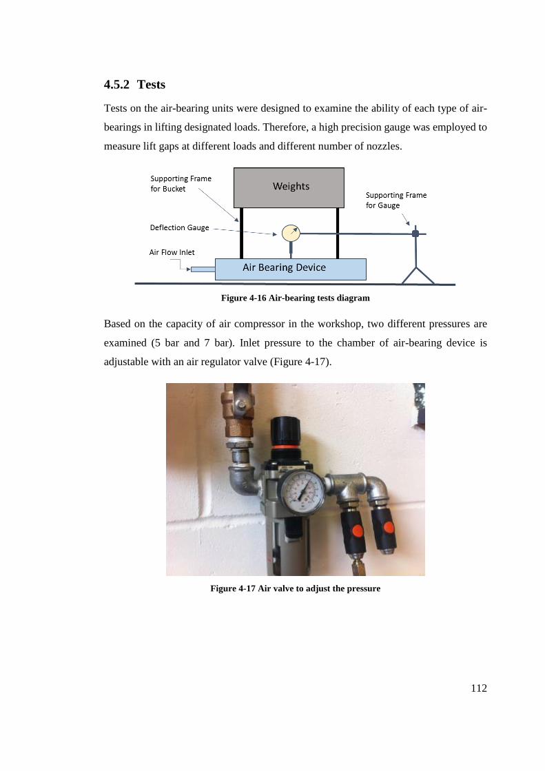
112
4.5.2 Tests
Tests on the air-bearing units were designed to examine the ability of each type of air-
bearings in lifting designated loads. Therefore, a high precision gauge was employed to
measure lift gaps at different loads and different number of nozzles.
Figure 4-16 Air-bearing tests diagram
Based on the capacity of air compressor in the workshop, two different pressures are
examined (5 bar and 7 bar). Inlet pressure to the chamber of air-bearing device is
adjustable with an air regulator valve (Figure 4-17).
Figure 4-17 Air valve to adjust the pressure

113
4.5.3 Experimental results
Nozzle type: In order to validate the results from numerical study, which shows the best
performance of 2-6mm diameter nozzle, three different nozzle types (Figure 4-12) were
tested in the workshop with different loading on top of the air-bearing device and
recording the vertical lift read by the gauge. Table 4-3 shows the performance of air-
bearing device for three different types of nozzle with different loadings on 5 bar
pressure.
Table 4-3 Lifting capacity of each nozzle type
investigated by experiments
Nozzle type (Din – Dout)
2 – 3 2 – 6 2 – 12
Weight (kg)
Lift (mm)
1.61 0.7 0.95 0.52
2.0 0.45 0.68 0.39
2.2 0.41 0.55 0.37
2.4 0.38 0.48 0.35
22.6 0.26 0.28 0.26
It is understood that the best performance belongs to the nozzle 2-6 as it provides the
highest lift among others in the same pressure inlet.
Figure 4-18 Lift against Weight diagram and trend lines for three different nozzles
1 1.6 kg is the self-weight of the device
00.10.20.30.40.50.60.70.80.9
11.11.2
0 5 10 15 20 25
Lift
(m
m)
Weight (kg)
nozzle 2-6
nozzle 2-12
nozzle 2-3

114
Number of nozzles: In order to determine the optimum number of nozzles, the same
procedure for loading and measuring lifts are conducted. As the nozzle 2-6 showed the
best performance, this time tests are conducted just on the 2-6 type nozzle and for
different numbers of nozzle to the bottom plate of air-bearing device to optimise the
number of nozzles.
Three sets of test for this part includes:
- Just one nozzle to the centre of bottom plate is open
- One nozzle to the centre and 6 far around
- One nozzle to the centre and 12 nozzles around (Figure 4-15)
Table 4-4 Lifts corresponding to different loadings for air bearing with one nozzle at the centre
one nozzle at the centre
@ 7 bar @ 5 bar
Weight (kg)
Lift (mm)
vertical stiffness (N/m)
Lift (mm)
vertical stiffness (N/m)
1.6 0.72 21800 0.52 30184.62
3.6 0.66 53509.09 0.44 80263.64
5.6 0.61 90059.02 0.41 133990.2
Table 4-5 Lifts corresponding to different loadings for air bearing with one nozzle at the centre
and six nozzles far around
one nozzle at the centre + 6 far around
@ 7 bar @ 5 bar
Weight (kg)
Lift (mm)
vertical stiffness (N/m)
Lift (mm)
vertical stiffness (N/m)
1.6 1.09 14400 0.63 24914.29
3.6 0.63 56057.14 0.43 82130.23
5.6 0.55 99883.64 0.34 161576.5

115
Table 4-6 Lifts corresponding to different loadings for air bearing with one nozzle at the centre
and 12 nozzles around
one nozzle at the centre + 12 around
@ 7 bar @ 5 bar
Weight (kg)
Lift (mm)
vertical stiffness (N/m)
Lift (mm)
vertical stiffness (N/m)
1.6 1.82 8624.176 0.95 16522.11
3.6 0.99 35672.73 0.76 46468.42
5.6 0.73 75254.79 0.68 80788.24
Results from these tests show the best performance in terms of lifting capacity when all
nozzles are open.
Figure 4-19 Lifts against weights for three different distribution of nozzles to the bottom plate
Figure 4-19 shows how the changes in the number of nozzles for air bearing affect the
total gap lifts. With reference to the results from this set of tests, it is understood that the
0
0.2
0.4
0.6
0.8
1
1.2
1.4
1.6
1.8
2
1.6 3.6 5.6
Lift
(m
m)
Weight (kg)
7 bar pressure one nozzle
5 bar pressure one nozzle
7 bar pressure one nozzleand six far around
5 bar pressure one nozzleand six far around
7 bar pressure one nozzleand 12 around
5 bar pressure one nozzleand 12 around

116
device with 13 number of nozzles has the best performance in terms of lifting the
weights. However, the increase in number of nozzles can not necessarily benefit the
level of performance for this particular air bearing as the air bearing with one nozzle to
the centre and six nozzles far around produces less lifting than the air bearing with just
one nozzle to the centre does, in small loading conditions. This is because - in small
loadings - the gap between cylinder and the ground is high and it forces the air to escape
from six outer nozzles easier and hence, less effectiveness on producing lift. In such
circumstances one single nozzle in centre produces better lift.
The other purpose of this test has been the investigation of the effects of pressure on the
performance of air bearing. Therefore, two different pressure (5 and 7 bar) have been
examined on the options for the third nozzle arrangement (one at the centre and 12
around). Figure 4-20 shows the trends how the lifting capacity of a specific air bearing
can be different based on changes in pressure. The trends in this figure give an insight
into choosing a desire pressure when lifting larger loads. It is understood that 5 bar
pressure produces better consistency when larger loads are considered. This could be
due to lower gap height and negative influence of shock waves in 7 bar pressure
compared to the 5 bar pressure. Therefore, and based on these findings, 5 bar pressure
is chosen for dynamic tests on the structure.
Figure 4-20 Different pressures on air bearing with one nozzle at the centre and 12 around
00.20.40.60.8
11.21.41.61.8
2
0 1 2 3 4 5 6 7
Lift
(m
m)
Weight (kg)
7 bar pressure
5 bar pressure

117
4.6 Validation
Validation of the results from numerical study with respect to the results from
experimental observations is presented here.
4.6.1 Numerical study and experiments
The parameter which can be investigated in this part is Mass-flow rate. The defined
mass flow rate of the compressor, used for producing pressurised air, can be obtained
from its data sheets (appendix A.6 Air pump specifications). The actual mass flow rate
of the compressor is calculated with respect to the volume rate of flow given by its
manual as 1665 Litre per second at 5bar pressure. Since the mass density of air is known
(1.225 kg/m3), the actual mass flow rate of the flow is simply calculated as 0.034 kg/sec.
Comparing the numerical derived mass flow rates to the actual mass flow rate of
compressor, shows reasonable agreement and accuracy for numerical simulations.
Table 4-7 Comparison of mass flow rates (kg/s)
Nozzle type Numerical Actual Difference
2-3 0.0313 0.034 7.99% 2-6 0.0388 0.034 14.11% 2-12 0.0327 0.034 3.7%
Table above shows that there is less than 15% errors in all cases. Although, the
compressor data sheet does not provide mass flow rates for different pressure ratios
corresponding to different nozzle geometries, it is anticipated that there will be less error
in mass flow rate calculations if the data for different pressure ratio is available.
4.6.2 Numerical validations
To validate the numerical study, following tests were conducted.
4.6.2.1 Grid dependency
One of the most important parameters that affects accuracy of the CFD solutions is the
quality of numerical grid. Grid dependency tests has been conducted on all cases where

118
extra numbers of mesh did not provide any change to the solutions. It is important for
the refinement to be substantial and systematic. Systematic refinement means that the
grid is refined in all direction with the same ratio. The number of cells that are used for
these simulations were two, three and four million that the three-million cell showed the
best and robust results.
4.6.2.2 Y-plus distribution
The Boundary layer is almost laminar in viscous sub-layer and fully turbulent in log-
law region. As mentioned before turbulence models are valid for fully turbulent flows,
therefore semi empirical formulas “wall functions”, are used to model flow properties
between the wall and log-law region. In log-law region the profile is
𝑢+ =1
𝜅ln 𝑦+ + 𝐵 =
�̅�
𝑢𝜏 (4.39)
where 𝜅 is von Karman constant (𝜅 = 0.41), 𝑢𝜏 is the shear velocity given by 𝑢𝜏 =
√|𝜏𝑤|/𝜌 and 𝜏𝑤 is the shear stress at the wall, �̅� is the mean velocity parallel to the
wall, 𝐵 is an empirical constant related to the thickness of viscous sublayer and 𝑦+ is
dimensionless parameter which shows distance from the wall and is defined as
𝑦+ =𝜌𝑢𝜏𝑦
𝜇 (4.40)
In viscous sublayer 𝑢+ = 𝑦+ but in buffer layer where 5 < 𝑦+ < 30, neither law holds.
In buffer layer the effect of viscosity and turbulent are equally important.
For turbulence modelling spatial considerations are required for grid resolution near the
wall. 𝑦+ values need to be in log-law region; therefore, it was important to keep the 𝑦+
values around thirty. This has been achieved with especial consideration for near wall
meshes.
4.7 Conclusion
In this chapter design and development of the air-bearing device needed for
experimental study for the research were discussed. It was explained that how the

119
numerical modelling can help in saving time and costs for designing a device which
works with the principles of fluid’s flow.
According to the results obtained from controlled laboratory tests compared to those
obtained from numerical modelling, it was concluded that the best option for nozzle
conical shape is 2 mm diameter inlet and 6 mm diameter outlet. This conclusion stands
for the purpose of handling heavier load at the same pressure on the proposed geometry
for air-bearing device.
Although the numerical model has its own limitations such as lack of dynamic mesh
generator, it has been a useful tool for a comparative study which played a valuable role
to determine the size and shape of nozzles.
Findings from laboratory tests were considered as validations for numerical modelling.
The results from laboratory tests were further used for determination of the number of
nozzles being implemented on the air-bearing device. The optimum number and
position for nozzles were then chosen as 13 nozzles.
It was also concluded that the best pressure is 5 bar in comparison to 7 bar pressure (two
available stable levels of pressure can be provided in the lab) for taking larger loads.

120
5 Experimental study on the
model structure
5.1 Introduction
An original investigation has been undertaken in order to gain an insight into the
dynamic behaviour of the scaled model in practice. In this chapter, specifications of the
model and measurement devices, tests’ method, tests’ results and analysis of results are
presented. The empirical results from laboratory tests are used for validation of findings
from analytical analyses and further comparisons with numerical simulations.
5.1.1 Experimental study (general argument)
An experimental study is an investigation procedure performed to verify, disprove, or
establish the validity of a hypothesis. The experimental study is usually conducted to
test a particular conjecture which is defined as an expectation or assumption about how
a particular phenomenon or process works. However, in some cases, an experiment may
also be carried out without a specific prediction or expectation about what the
experiment is supposed to reveal. Experiments can also provide insight into reasons and
effects of a phenomenon by explaining what outcome occurs when a particular factor is
changed. The results of an experiment - if it is carefully conducted – can support or
disprove the hypothesis (Popper, 2002).
In the scientific methods of experimental studies, an experiment is an empirical
procedure that adjudicates between contending models or hypotheses (Cooperstock,
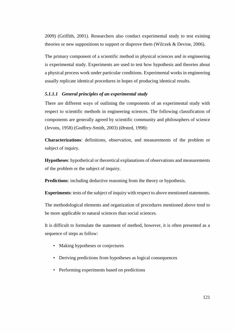
121
2009) (Griffith, 2001). Researchers also conduct experimental study to test existing
theories or new suppositions to support or disprove them (Wilczek & Devine, 2006).
The primary component of a scientific method in physical sciences and in engineering
is experimental study. Experiments are used to test how hypothesis and theories about
a physical process work under particular conditions. Experimental works in engineering
usually replicate identical procedures in hopes of producing identical results.
5.1.1.1 General principles of an experimental study
There are different ways of outlining the components of an experimental study with
respect to scientific methods in engineering sciences. The following classification of
components are generally agreed by scientific community and philosophers of science
(Jevons, 1958) (Godfrey-Smith, 2003) (Ørsted, 1998):
Characterizations: definitions, observation, and measurements of the problem or
subject of inquiry.
Hypotheses: hypothetical or theoretical explanations of observations and measurements
of the problem or the subject of inquiry.
Predictions: including deductive reasoning from the theory or hypothesis.
Experiments: tests of the subject of inquiry with respect to above mentioned statements.
The methodological elements and organization of procedures mentioned above tend to
be more applicable to natural sciences than social sciences.
It is difficult to formulate the statement of method, however, it is often presented as a
sequence of steps as follow:
• Making hypotheses or conjectures
• Deriving predictions from hypotheses as logical consequences
• Performing experiments based on predictions

122
5.1.2 Experimental study for this research
The purpose of this research is defined as introduction of an innovative system for
seismic base isolation. The new system which was introduced in chapter 3 is based on
the advantages of air bearing for isolation. This is supported by the theory of producing
a thin layer of air underneath of a structure and above its base to decouple the structure
from horizontal movements. In order to predict the behaviour of the structure in isolated
conditions, the analytical model was introduced and explained in chapter 3. For
supporting the hypothesis experimental study has been conducted and will be explained
in details in this chapter.
The method for the experimental study in this research is in accordance with the general
principles mentioned in the previous section as follow:
5.1.2.1 Formulating the question
The question can be very specific in scientific methods of experimental study. In this
research the key question arose from the gap of the knowledge with respect to the
dynamic behaviour of structures under earthquake loadings. That is finding a better way
of seismic isolation which overcome the drawbacks of current system along with
keeping the advantages known for those systems. The new system then was defined with
respect to the principles of seismic isolations (i.e. lengthening the fundamental period
and imposing some levels of damping) and state of the art technology (i.e. air bearing
and early warning system).
5.1.2.2 Hypothesis
A hypothesis is defined based on the knowledge obtained through formulating the
question. The hypothesis might be very specific, or be the desired outcome.
“A scientific hypothesis must be falsifiable, meaning that one can identify a possible
outcome of an experiment that conflicts with predictions deduced from the hypothesis;
otherwise, it cannot be meaningfully tested” (Popper, 2002).
Hypothesis in this study explain the dynamic behaviour of the scaled model structure in
which it is assume that the response of the structure to dynamic loads are reduced and

123
damages are alleviated. The hypothesis is defined based on stablished theories of
structural analysis.
5.1.2.3 Prediction
Determining the logical consequences of the hypothesis is involved in this step. It is
typical to select one or more predictions and conduct further testing. In this research,
the fundamental frequencies and periods of a structure and structural response
(displacement and acceleration) were predicted through an analytical model analysis,
and damping was to be measured as unpredicted value.
5.1.2.4 Testing
Experimental test involves investigation of whether the real world behaves as predicted
by the hypothesis. The purpose is to determine whether observations of the real world
are in agreement or disagreement with the predictions derived from a hypothesis. In this
research the relevant dynamic tests were conducted to determine the fundamental
frequencies of the structure in isolated and unisolated modes and to perform a
comparative study on the response of the structure in two different conditions of base
(fixed and isolated) with applying three different loadings.
5.1.2.5 Analysis
Analysis determines what the results of conducted tests show and what they mean to the
researcher. The analysis of results decide if the evidence has falsified the hypothesis or
they support the hypothesis. In this research, the analyses were performed on the results
obtained from tests and consequently, the final conclusion on whether the evidences are
strong enough, to support the robustness of the new proposed isolation system, was
drawn.

124
5.2 Test rig
The test rig configuration comprises of the scaled structure and proposed isolation
system. The proposed test rig satisfies the following criteria:
Tests are suitable for the scaled model.
Tests replicate the same vibration observed in the real conditions.
The structure does not experience unrealistically high loading that might change
the failure mechanism.
The test specification is suitable for laboratory based testing and appropriate for
analytical and numerical modelling evaluations.
In this research free vibration tests on the scaled structure are considered in order to
observe the dynamic behaviour of the scaled structure to compare with analytical and
numerical simulations.
5.3 Dynamic test
Dynamic tests involve measuring the dynamic response of a structure to excitation. This
includes free vibration tests and force vibration tests.
There are different methods of generating excitation for free vibration test. The simplest
way is employing ambient excitation, produced from earthquake, wind or traffic. The
main drawback in this approach is the lack of control over amplitude, direction and
duration of applied loading. Another approach is the snap-back test in which a structure
is suddenly released from an imposed initial loading or displacement and the ensuing
free vibration recorded in terms of acceleration or displacement (Butterworth, et al.,
2004).
The most well-known force vibration test is shaking table test, in which a mechanical
exciter applies a varying force of known frequency and amplitude to a designated
basement on which the structure is mounted. Shake tables for dynamic test purposes are
also able to produce simulated ground motions, including reproduction of previous
earthquake records.

125
With respect to the aims and objectives of this research, the scope of experimental study
was defined to
• verify the fundamental frequency of the structure,
• perform a comparative study on the maximum acceleration and story drifts
exerted in the structure due to similar loading conditions and different base
configuration (isolated and unisolated), and
• extracting damping properties of the structure.
In order to accomplish these pre-defined goals, the method of snap-back test is chosen
for dynamic tests (Figure 5-1). As it is shown in figure below, an initial displacement
(due to the hanged mass) is applied on top of the structure. As a result of a sudden release
of the mass (cutting the rope) the structure vibrates on its natural frequency (free
vibration).
Figure 5-1 Schematic view of the snap-back test
In order to observe the performance of the proposed isolation system designed for the
scaled structure, it is necessary to investigate the dynamic behaviour of the structure. To
u0
mass
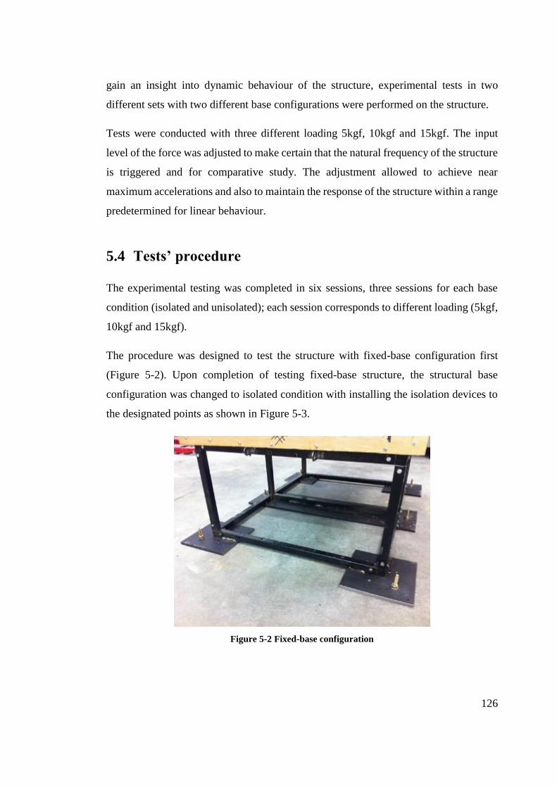
126
gain an insight into dynamic behaviour of the structure, experimental tests in two
different sets with two different base configurations were performed on the structure.
Tests were conducted with three different loading 5kgf, 10kgf and 15kgf. The input
level of the force was adjusted to make certain that the natural frequency of the structure
is triggered and for comparative study. The adjustment allowed to achieve near
maximum accelerations and also to maintain the response of the structure within a range
predetermined for linear behaviour.
5.4 Tests’ procedure
The experimental testing was completed in six sessions, three sessions for each base
condition (isolated and unisolated); each session corresponds to different loading (5kgf,
10kgf and 15kgf).
The procedure was designed to test the structure with fixed-base configuration first
(Figure 5-2). Upon completion of testing fixed-base structure, the structural base
configuration was changed to isolated condition with installing the isolation devices to
the designated points as shown in Figure 5-3.
Figure 5-2 Fixed-base configuration
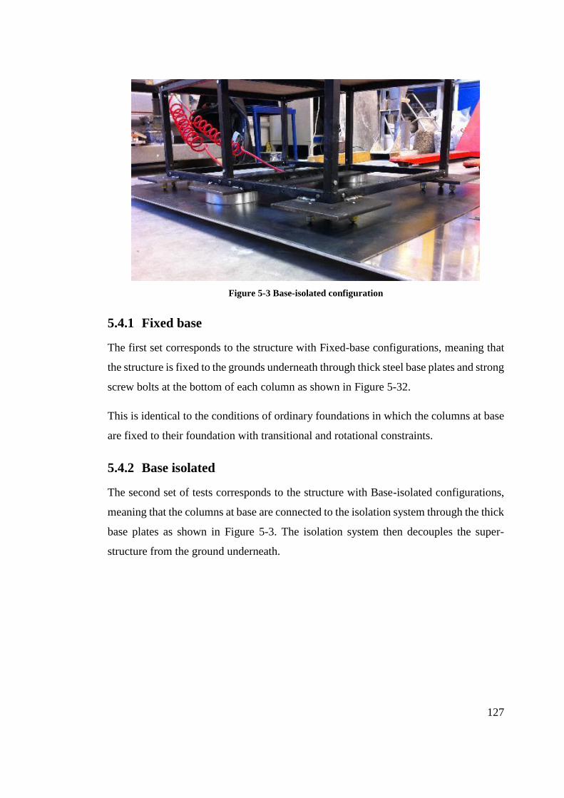
127
Figure 5-3 Base-isolated configuration
5.4.1 Fixed base
The first set corresponds to the structure with Fixed-base configurations, meaning that
the structure is fixed to the grounds underneath through thick steel base plates and strong
screw bolts at the bottom of each column as shown in Figure 5-32.
This is identical to the conditions of ordinary foundations in which the columns at base
are fixed to their foundation with transitional and rotational constraints.
5.4.2 Base isolated
The second set of tests corresponds to the structure with Base-isolated configurations,
meaning that the columns at base are connected to the isolation system through the thick
base plates as shown in Figure 5-3. The isolation system then decouples the super-
structure from the ground underneath.

128
5.5 Measurement devices
The measurement devices were provided by a Swiss company namely GeoSIG,
specialist in dynamic measuring and structural monitoring solutions. The measurement
devices’ are listed below with details of their functionality.
5.5.1 Data acquisition
GMSplus as the latest generation of GeoSIG measurement systems is used for acquiring
data from accelerometers. The main advantages can be summarised as high
performance, flexibility in operation and enhanced connectivity. The instrument is
equipped with software which processes data in real time. As a self-contained
instrument GMSplus is supplied with an uninterruptible power-supply (A 12 VDC, 7.0
Ah battery), which can provide more than 24 hours autonomy. The external power
supply cable (100-240 VAC) will be used to connect the instrument to the main. The
instrument is capable of being connected to a desktop or laptop through its ports and
relevant cable. It includes an ethernet cable and connector to ensure fast and reliable
data transfer (GeoSIG, 2015). Full specifications and certificate of calibration are given
in appendix A.7 GMSplus specifications and calibration.
5.5.2 Sensors
Accelerometers have been chosen as the sensor of measurements, as acceleration
recorded data are easily convertible to other parameters such as velocity and
displacement. AC-43 accelerometer types are used for acceleration measurements with
full scale range of ±2g and up to 100Hz bandwidth. The accelerometer type is MEMS
Force Balance Accelerometer with dynamic range of 95dB. The AC-43 accelerometer
works based on the modern MEMS (Micro Electro-Mechanical Systems) technology,
in which sensing cells are assembled in a way that optimizes their performances. MEMS
cells include linear accelerometer sensing elements which measure the capacitance
variation in response to any movement or inclination and a factory trimmed interface
chip that converts the capacitance variations into analogue or digital signal proportional
to the motion (GeoSIG, 2013). Sensors should be tested and calibrated prior to start the
tests to ensure reliable data records. Hence, accelerometers verification tests and

129
calibrations have been carried out by GeoSIG. Full specifications and calibration
certificates are given in appendix A.8 Accelerometer specifications and calibration.
5.5.3 Data communication software
The software used for data communication is GeoDAS, the product of GeoSIG. The
software enables users to obtain recorded data and view the diagrams and perform some
analyses. The program is basically used for acquisition of data provided by any standard
GeoSIG instrument and also for instrument configuration. An RS-232 cable with USB
converter is provided along with the software for communication between data
acquisition system and computer.
5.6 Data analysis and results
By analysing signals from measurement devices, one can learn more about the nature of
the vibration of the structure. Data analysis in this case is basically divided into two
parts; Time domain and frequency domain analysis; each of which provides a different
view or insight into the mechanism of the vibration of the structure.
Time domain analysis is the study of signals (accelerations or displacement records) as
a function of time. The plot of vibration parameters (acceleration, velocity or
displacement) versus time provides information needed for characterization of the
dynamic behaviour of a structure in terms of detecting the peaks levels or identifying
the periods and furthermore, estimating the decay rate. These are known as the typical
results of time domain analysis.
Frequency domain analysis refers to the study of signals as function of frequency
which provides the plot of vibration parameters (or square root of them or other common
types of representation) versus frequency. It is possible to transform any time history
signal into the frequency domain. The most well-known mathematical transformation
technique of time signals is Fourier Transformation after the French mathematician
Jean-Baptiste Joseph Fourier (Sterken, 2003). Fourier Transform is based on the
assumption that any periodic signal can be represented in the form of a series of sine

130
waves; each of which has its own frequency and peaks. In vibration analysis of a
structure, these peaks and their frequencies are important and meaningful.
The next sections discuss the vibration data obtained from the experimental tests on the
scaled structure. The data are represented in the form of acceleration and displacement
signals in time domain and analysed data in frequency domain.
5.6.1 Absolute acceleration on top of the structure
In this section, the experimental results are presented in the form of a comparison of the
absolute acceleration on top of the structure due to specific loading in both fixed base
and isolated conditions. As mentioned before three snap-back test runs were performed
for each base condition which included a specific load in magnitude (5kgf, 10kgf and
15kgf) applied to the structure in order to ensure that the first two fundamental
frequencies of vibration are triggered; and to check the effects of increase in applied
load on natural frequencies for further validations.

131
Figure 5-4 Acceleration on top of the structure in horizontal direction due to 5kgf snap-back test
(Fixed-base); maximum absolute value = 36.96 cm/s2
Figure 5-5 Acceleration on top of the structure in horizontal direction due to 10kgf snap-back test
(Fixed-base); maximum absolute value = 60.65 cm/s2
Figure 5-6 Acceleration on top of the structure in horizontal direction due to 15kgf snap-back test
(Fixed-base); maximum absolute value = 126.82 cm/s2
Figure 5-4 to Figure 5-6 show the magnitude of accelerations on top of the structure (5th
story) due to application of 5kgf, 10kgf and 15kgf respectively in horizontal direction
in snap-back tests. Figure 5-7 illustrated how the maximum acceleration experienced on

132
top of the structure can be affected by magnitude of applied load. As it was expected,
the greater the applied load in snap-back test, the greater magnitude of acceleration is
exerted to the structure. This further confirms the consistency of the structural system
of the scaled model.
Figure 5-7 The effects of applied load magnitudes in accelerations experienced on top of the
structure (Fixed-base conditions)
It is understood that the maximum absolute acceleration is increased by 77% when the
applied load is increased by 100% from 5kgf to 10kgf; likewise the increase in
acceleration is 270% when the applied load is increased by 300% from 5kgf to 15 kgf.
By changing the conditions of base from fixed to isolated, it is expected that the
maximum absolute acceleration exhibits some levels of reduction. Figure 5-8 to
Figure 5-10 show how the acceleration experienced on top of the structure is reduced
thanks to the new base isolation system. Reduction in levels of acceleration on the
structure is a must for any seismic isolated system and as it was discussed earlier, base
isolation solution is the best known way of practice in this area. It was observed that the
present isolation system exhibits a great performance in reduction of absolute
acceleration and therefore, is able to reduce the potential structural damage.

133
Figure 5-8 Acceleration on top of the structure due to 5kgf in snap-back test;
Fixed base (FB) and Base isolated (BI) conditions
Figure 5-9 Acceleration on top of the structure due to 10kgf in snap-back test;
Fixed base (FB) and Base isolated (BI) conditions
Figure 5-10 Acceleration on top of the structure due to 15kgf in snap-back test;
Fixed base (FB) and Base isolated (BI) conditions

134
Results of acceleration response confirms the reduction of 28%, 51% and 49% in
absolute acceleration in snap-back test for 5kgf, 10kf and 15kgf respectively. Therefore,
the present isolation system demonstrates adequate level of isolation and exhibit a great
performance against horizontal input. The performance of the structure against different
types of earthquake is investigated through numerical simulation and results are given
and discussd in the next chapter.
5.6.2 Natural frequencies and periods
The natural frequencies of a structure demonstrate the sensitivity of the structure to
different loading frequencies. If the loading frequencies coincide with the natural
frequencies of a structure, its vibration increases dramatically which increase the
acceleratin in the structure (resonance). In order to reduce the resonance effect, one way
is to shift the fundamentl fresquency of the structure to a smaller one. Base-isolation
systems - if applied appropriately – can shorten the natural frequency of vibration of the
structure to smaller one (far from the devastating frequency of earthquake shocks) by
providing a layer of low horizontal stiffness to the base of the structure. This is
investigated in this chapter by anlysis of the data obtained from experimental laboratory
tests on the scaled structure in the workshop.
Data analysed in the last section were in time domain; if data in time domain are
transferred to frequency domain with using Fast Furier Transformation, it is possible to
analyse data in frequency domain and the analysis is called Frequency Response
Analysis. The peaks in frequency response diagrams then reperesent the natural
frequency of vibration of the structure (Avitabile, 2001).
5.6.2.1 Fast Fourier Transformation (FFT)
FFT is refered to as the discrete Fourier Transform (DFT) of a collected block of time
signal which represents the frequency spectrum of the time signal. It computes the DFT
of a sequence rapidly by factorizing the DFT matrix into a product of mostly zero factors
(Ramirez, 1975). In order to transform real data readings from time domain to frequency
domain it is necessary to know the number of points, intervals and sampling rates
(Harris, 1978). The time-frequency relationship is as follow:

135
- if data is sampled at N equi-spaced points in time domain, where n = 0, 1, …, N-
1, then the time signal consists of N real numbers; therefore, if the time interval
between samples is known as dt, the total length of the sample record is T and
T= N.dt.
- if the sampling rate (the number of readings per time unit) is equal to fs, there
will be fs/2 number of data at positive frequencies and fs/2 number of data at
negative frequencies where, fs=N/T.
- if the frequency resolution (frequency separation of the data points) is considered
as df , the bandwith (the maximum frequency of the display) is equal to Fmax and
Fmax = fs/2 = (N/2).df.
therefore, the time and frequency domain relationship is defined as
𝑑𝑡 = 1
2𝐹𝑚𝑎𝑥 (𝑠𝑒𝑐𝑠) (5.1)
𝑑𝑓 =1
𝑇 (𝐻𝑧) (5.2)
In the laboratory tests conducted for this study, accelerometers with sampling rate of 50
per seconds are used which determines the time increemnts of 0.02s and the bandwith
of 25Hz. The algorithm of FFT and MATLAB implementation code for frequency
response analysis of this part is given in appendix A9.
The results from FFT analysis of acquired data from snap-back tests on the scaled
structure are presented here with relevant discussion. The most important understanding
from frequency response analysis is perhaps, detection of fundamental frequency of
vibration. This is the position of the peaks (regardless of its unit) on the frequency axis
and is obtainable by analysing the recorded displacement values on top of the structure
(5th story). Figure 5-11 demonstrates the fundamental frequencies of the structure in
fixed-base (FB) and base-isolated (BI) conditions.

136
Figure 5-11 The effect of isolation system in shifting the fundamental frequency of the structure to
a lower one
It is understood from Figure 5-11 that the isolation system shifts the fundamental
frequency of the structure to a smaller one. It means that the isolation system shifts the
fundamental period of vibration of the structure to a longer one from 0.228s to 0.855s.
Therefore, the adequate isolation performance of the system is confirmed.
The results are also in accordance with what were expected from analytical model of
the structure presented in chapter 3 of this dissertation. It was predicted that the
fundamental periods of the structure in fixed-base and base-isolated conditions should
be around 0.204s and 0.827s respectively (section 3.6.2). It is now confirmed that the
fundamental periods of the vibration of the structure are 0.228s and 0.855s for fixed-
base and base-isolated respectively. The results of experimental study therefore show
the difference of 10% for fixed-base and 3.3% for base-isolated conditions in the value
of fundamental periods in comparison to the analytical model of the structure.
It is understood from the diagram of frequency response in Figure 5-11 that the
maximum displacement on top of the structure is increased in isolated structure. This
increase in displacement was predictable as adding a layer of low stiffness to the base
of the structure, simply means that the maximum absolute displacement on each story
tends to increase with respect to the fact that the isolation stiffness is considerably lower
than the stiffness of each story. Therefore, it is expected that the structure moves more
like a rigid body when isolated. This can be observed when considering the displacement
response of the top three stories at their peaks.

137
5.6.3 Story drifts
Inter – story drifts is defined as the relative displacement between two adjacent stories
at a certain time and is known as one of the important causes of structural damage (Wu
& Samali, 2002). In order to gain an insight into the performance of the structure when
subject to a certain loading condition in fixed-base and base-isolated settings, the
relative displacements are investigated and comapred. By double integration of
acceleration values obtained from accelerometer readings, the displacement values are
calculated.
Figure 5-12 Displacement values on top three levels of the structure in snap-back test (5kgf), in
Fixed-base condition
Figure 5-13 Displacement values on top three levels of the structure in snap-back test (5kgf), in
Base-isolated conditions

138
Table 5-1 Story drifts on top of the structure in Fixed-base (FB) and Base-isolated (BI) conditions
in snap-back test with 5kgf
FB Displacement
(mm)
Drifts (mm) BI Displacement
(mm)
Drifts (mm)
Story Story
5th 0.738 0.099 5th 0.956 0.015
4th 0.639 0.124 4th 0.941 0.037
3rd 0.515 - 3rd 0.904 -
Figure 5-12 and Figure 5-13 are depicting the graph of displacement values in time
domain when the structure is subject to the same loading conditions and different base
configurations. Table 5-1 shows the values of absolute displacements on top three levels
of the structure and calculated story drifts.
It can be seen that the base-isolated model demonstrates a dramatic reduction in the
story drifts. These are 85% reduction for fith story and 70% for the fourth story. This
reduction implies that there would be a much lower level of structural damage in isolated
structure compare to unisolated structure when the structure is subject to a horizontal
load as a result of the reduction in horizontal relative displacement exerted in the
structure.
Figure 5-14 and Figure 5-15 show the displacement time-history response of the
structure on top three stories and Table 5-2 compares the results. Great reductions in
story drifts are again observed; the story drift coresponds to the 5th story demonstrates
43% reduction in isolated conditions compare to unisoalted conditions. Likewise the
drift coresponds to 4th story is reduced by 41%.
In order to gain an insight into the sensitivity of structure to greater loading in snap-back
test, the tests have been run for 15kgf and the results are shown in Figure 5-16 and
Figure 5-17; the comparisson of results are given in Table 5-3.
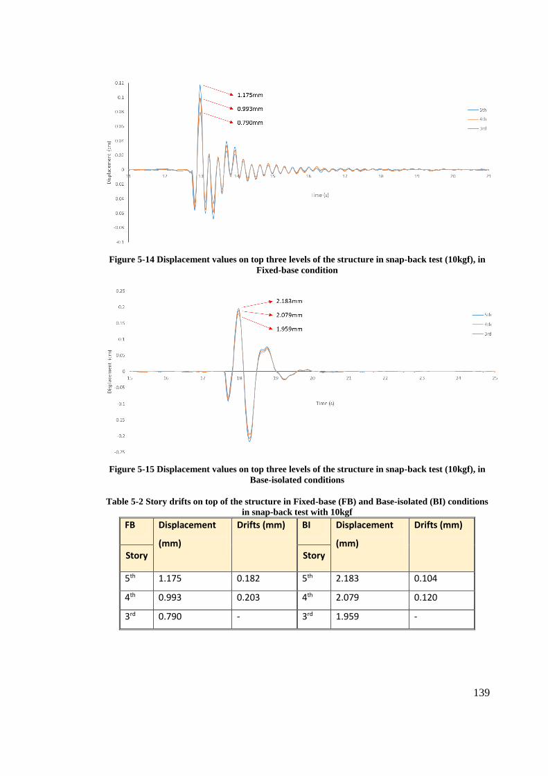
139
Figure 5-14 Displacement values on top three levels of the structure in snap-back test (10kgf), in
Fixed-base condition
Figure 5-15 Displacement values on top three levels of the structure in snap-back test (10kgf), in
Base-isolated conditions
Table 5-2 Story drifts on top of the structure in Fixed-base (FB) and Base-isolated (BI) conditions
in snap-back test with 10kgf
FB Displacement
(mm)
Drifts (mm) BI Displacement
(mm)
Drifts (mm)
Story Story
5th 1.175 0.182 5th 2.183 0.104
4th 0.993 0.203 4th 2.079 0.120
3rd 0.790 - 3rd 1.959 -

140
Figure 5-16 Displacement values on top three levels of the structure in snap-back test (15kgf), in
Fixed-base condition
Figure 5-17 Displacement values on top three levels of the structure in snap-back test (15kgf), in
Base-isolated conditions
Table 5-3 Story drifts on top of the structure in Fixed-base (FB) and Base-isolated (BI) conditions
in snap-back test with 15kgf
FB Displacement
(mm)
Drifts (mm) BI Displacement
(mm)
Drifts (mm)
Story Story
5th 2.474 0.379 5th 3.129 0.177
4th 2.095 0.432 4th 2.952 0.202
3rd 1.663 - 3rd 2.750 -

141
It is once again confirmed that the story drifts are reduced significantly (by 53% in both
5th and 4th level) in isolated structure. This implies that reduction in story drifts is an
indisputable advantage of the proposed isolated system.
A comparison between the values of story drifts of structure subject to different amount
of loadings suggests that the structure is more sensitive to the increase in loading when
it is isolated. This will be investigated in the next chapter based on the results of
numerical simulation of the structure subject to different earthquakes.
5.6.4 Damping
Damping values are empirical values that must be obtained by measurements. Damping
is recognised as playing a major role in reduction of response and alleviation of the level
of damage in a given structure. Even though, damping has been remained the most
difficult dynamic property of the structure to predict when designing the structure.
Unlike mass and stiffness, damping cannot be deducted from the physical property of
the structure (Butterworth, et al., 2004). Accordingly, the assessment of damping relies
mostly on measured data from experimental observations on the given structure or
similar structures.
Figure 5-18 Effects of damping in response of the structures, where D denotes the response of the
structure and 𝜷 is the ratio of applied loading frequency to the natural free-vibration frequency
(Clough & Penzien, 2003)

142
A structure with relatively low damping and with a natural frequency close to the natural
frequency of the applied dynamic load could produce high level of damage under
resonance conditions.
5.6.4.1 Definition
Damping in dynamic systems is defined as the phenomenon by which mechanical
energy is dissipated (De Silva, 2007). The dissipated energy is usually converted into
internal thermal energy. It is very important to gain a knowledge about the level of
damping in a given structure. Damping properties will be used in structural analysis and
further in structural tests and utilisations. Therefore, in order to develop a realistic
dynamic model of a structure, the nature and level of damping should be known. It is
also essential to have a good knowledge of system’s damping when imposing dynamic
environmental limitations is considered. The dynamic limitations involve maximum
dynamic excitation the system can withstand under service conditions (De Silva, 2007).
Moreover, knowledge of a system’s damping is useful in making design modifications
in systems with failure in acceptance tests.
In general, damping occurs through the dissipation of mechanical energy in vibrating
system. Types of damping includes:
• Structural damping
• Material internal damping (viscoelastic and hysteretic)
• Viscous damping
• Interface damping
• Fluid damping
• Coulomb friction
• Stribeck damping
It is customary to represent various types of damping using equivalent viscous damping.

143
5.6.4.2 Measurement of damping
Two different approaches are known for measurement of damping in structures when
time-history response of the structure is available; time domain method and frequency
domain method.
In time domain methods the response of a structure which could be acceleration,
velocity, or displacement is considered over a certain period of time. The damping ratio
is then obtainable by employing relevant theories in vibration and appropriate
calculations. There are three accepted methods for extracting damping from time history
response of a structure (De Silva, 2007):
Logarithmic decrement method
Step-Response method
Hysteresis loop method
In frequency domain methods the response of a structure versus different frequencies is
considered as the source of calculations. Widely accepted methods of this approach are
listed below (De Silva, 2007):
Magnification factor method
Bandwidth method
For structural analysis purposes when data of time-history response is available the most
convenient way of estimating damping is Logarithmic decrement method. This method
is used to measure the overall damping of a structure in this research.
5.6.4.3 Logarithmic decrement method
The method is perhaps the most popular one when using experimental data for
measurement of damping. This method is basically used for single-degree-of-freedom
(SDOF) systems but it can be also used for multiple-degree-of-freedom (MDOF) system
when lower modes are targeted (Butterworth, et al., 2004).
When a system is excited by an impulse input which can be an initial condition
(displacement or force), the system response takes the form of a time decay as
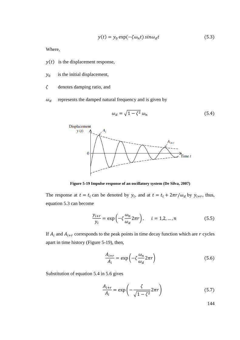
144
𝑦(𝑡) = 𝑦0 exp(−𝜁𝜔𝑛𝑡) 𝑠𝑖𝑛𝜔𝑑𝑡 (5.3)
Where,
𝑦(𝑡) is the displacement response,
𝑦0 is the initial displacement,
𝜁 denotes damping ratio, and
𝜔𝑑 represents the damped natural frequency and is given by
𝜔𝑑 = √1 − 𝜁2 𝜔𝑛 (5.4)
Figure 5-19 Impulse response of an oscillatory system (De Silva, 2007)
The response at 𝑡 = 𝑡𝑖 can be denoted by 𝑦𝑖, and at 𝑡 = 𝑡𝑖 + 2𝜋𝑟/𝜔𝑑 by 𝑦𝑖+𝑟, thus,
equation 5.3 can become
𝑦𝑖+𝑟
𝑦𝑖= exp (−𝜁
𝜔𝑛
𝜔𝑑2𝜋𝑟) , 𝑖 = 1,2, … , 𝑛 (5.5)
If 𝐴𝑖 and 𝐴𝑖+𝑟 corresponds to the peak points in time decay function which are 𝑟 cycles
apart in time history (Figure 5-19), then,
𝐴𝑖+𝑟
𝐴𝑖= exp (−𝜁
𝜔𝑛
𝜔𝑑2𝜋𝑟) (5.6)
Substitution of equation 5.4 in 5.6 gives
𝐴𝑖+𝑟
𝐴𝑖= exp (−
𝜁
√1 − 𝜁22𝜋𝑟) (5.7)

145
Then, the logarithmic decrement 𝛿 is given by
𝛿 =1
𝑟ln (
𝐴𝑖
𝐴𝑖+𝑟) =
2𝜋𝜁
√1 − 𝜁2 (5.8)
And damping ratio may be expressed as
𝜁 =1
√1 + (2𝜋/𝛿)2 (5.8)
For low damping ratios (typically under 10%), when 𝜔𝑑 ≅ 𝜔𝑛 the above equation
becomes (De Silva, 2007)
𝜁 =𝛿
2𝜋 (5.9)
Alternatively, when 𝑛 cycles of damped vibration are needed for the amplitude to decay
by a factor of 𝑘𝑑, in low damping (𝜁 < 0.1)
𝜁 =1
2𝜋𝑛ln(𝑘𝑑) (5.10)
5.6.4.4 Results
The method of logarithmic increment is employed to measure overall damping of the
structure for two different base configurations and three different impulse loadings.
Figure 5-12 to Figure 5-17 are considered to determine the level of damping in each test.
Results are presented in Table 5-4.
Table 5-4 Damping ratios extracting from displacement response of the structure
Bas
e co
nd
itio
n
s
Snap-back test loading (kgf)
Damping ratio (𝜻) (% of critical)
Fix
5 5.9
10 5.8
15 6.5
Iso
late
d 5 12.3
10 12.4
15 13.5

146
The above table reveals how the isolation system benefits the dynamic behaviour of the
structure by damping the free vibrations (induced by an impulse force) and alleviation
of shocks. The damping ratio is increased drastically for isolated structure, which is the
direct result of isolation system. The unisolated structure exhibits around 6% damping
ratio which is a reasonable level for a structure of this kind and the isolated structure
shows 12% damping as a result of employing isolation system. The overall damping in
the isolated structure is, indeed, the result of combination of structural damping and
isolation system damping, yet it should not be confused with the sum of the two damping
ratio. This means that the difference in the level of overall damping in the isolated
structure compare to the unisolated structure (around 6%) does not necessarily denote
the damping of isolation system (De Silva, 2007).
The table shows that there has been a slight increase in the level of damping when the
applied force is increased. This is, in fact, due to the greater movement exerted in the
structure due to greater loads and therefore, greater internal friction which produces
more damping. This is in a good agreement with the work of Butterworth, et al. in 2004
(Butterworth, et al., 2004).
As it was discussed before, damping is beneficial for isolation systems. Any isolation
system should demonstrate an increase in the level of overall damping in the given
structure in practice. In this section it was shown - by the results obtained from practical
tests – that the proposed isolation system provides the structure with a reasonable level
of damping in vibrations. The empirical values of damping obtained from experimental
tests will be further used in numerical simulation of the structure.
5.7 Conclusion
This chapter described and discussed the experimental study - the major part of this
research - on a case study which is a scaled model of a five-story building. It was
explained that how a hypothesis can be conducted in a scientific method through an
experimental investigation.
147
The methods of experimental tests explained in this chapter can be used for further study
as the followed approach (snap-back test) is categorised as a low-cost yet powerful
procedures for extracting the dynamic parameters of a given structure.
The results from experimental study validated the findings from analytical model of the
structure explained earlier in chapter 3. It was shown that the proposed isolation system
is able to lengthen the fundamental period of a structure to a greater one which results
in diminution in the level of peak acceleration exerted to the structure. It was also
discussed that, however, the maximum displacement on top of the structure is increased
by using the isolation system, story drifts are reduced by more than 40% in all cases
(given loading conditions). Damping as an empirical parameter was measured with
respect to the time-history response of the structure and employing Logarithmic
decrement method. It was conclude that the proposed isolation system is able to increase
the overall damping ratio from around 6% to 12%. The measured values for damping
are further employed in numerical simulation.
In the chapter that follows, the numerical model of the building is described and the
performance of the proposed isolation system under different earthquakes is
investigated accordingly.

148
6 Computer simulation of
the structure
6.1 Introduction
The numerical method enables researchers and engineers to solve complicated sets of
equations and variables with numbers of constraints which all together define a problem.
The time-history model of a structure is a mathematical model that uses numerical time-
stepping procedure to obtain the structural behaviour over time. This will be a numerical
simulation of sets of governing differential equations, obtained from physical
parameters of the structure that cannot be solved analytically.
In investigation of the dynamic behaviour of a structure, it is common to generate a
numerical simulation for a given building with respect to the development of computer
technology these days. When study of the dynamic behaviour of a structure subjected
to an earthquake or wind loads is considered, the best method is to examine a scaled real
model of the given structure under scaled given loading. This approach which is possible
through the use of shaking table in special fitted laboratories enable researchers to obtain
the exact results. The drawback is that such facilities are not available everywhere and
for everyone. In addition it is not possible and it is not rational to build a physical model
for every given building. Therefore, the mathematical model of a structure is generated
with respect to established physics laws. The physical model of the structures then can
be represented with a mathematical model.

149
The mathematical model of a structure should be accurate and should simplify the
problem with respect to the importance of parameters. Then the given problem is
represented by sets of equations, variables and unknowns. The mathematical models of
structures in dynamic analysis are not always simple to analyse as in majority of cases
there are numbers of simultaneous differential equations to be solved. The analytical
approach for solving the system of equations in these cases is almost impossible.
Therefore, numerical methods are employed to solve the sets of equations and unknowns
for a given problem.
The researcher or engineer who is looking at a problem in structural analysis can
generate their own approach for a numerical solution of the given problem. However,
there are programs and software available to be employed. One of the most powerful
tools is SAP2000 which enables the user to perform dynamic analysis on a structure
with respect to variety of parameters. One of the features this program provides is the
use of previous earthquake records. The user can examine the target structure’s dynamic
behaviour under different past earthquake records. It is also possible to define an
arbitrary dynamic loading in terms of force, acceleration or displacement to the program.
Hence, the performance of a given structure can be investigated under the other
earthquake records which are not available in the program predefined records.
In this research the numerical modelling of the structure is generated to gain an insight
into its dynamic behaviour with and without proposed isolation system under different
earthquakes. For this purpose, SAP2000 is chosen as the numerical simulator and
analyser tool with respect to its ability in dynamic analysis.
The earthquake records are scaled by factor of 0.316 in time axis (according to scaling
analysis, Table 3-1) to maintain the dynamic resemblance between the scaled model and
real scale structure. The earthquake records are chosen from the records of past
earthquakes with respect to their magnitude and duration.

150
6.2 Physical model
The physical model is what was explained in chapter 3, a scaled structure comprises of
five story, in which the stories are linked through the columns.
Figure 6-1 Physical model of the structure (dimensions in mm)
For simplification of the model in analysis, the structure is simulated as a shear building
explained in section 3.6. (Figure 6-2).
Figure 6-2 shear building model of the structure for dynamic analysis (direction of movement is
shown)

151
Therefore, the model of the structure for analysis is comprises of masses which are
connected through springs with relevant stiffness values.
6.3 Mathematical model
For the mass-spring model of the given structure the governing equations are defined
by recalling equation 3.3 as
𝑀�̈� + 𝑐�̇� + 𝐾𝑢 = −𝑀�̈�𝑔 (6.1)
Where, 𝑀, and 𝐾 represent mass and stiffness matrix respectively as
𝑀 =
[ 40 0 0 0 00 40 0 0 00 0 40 0 00 0 0 40 00 0 0 0 40]
(𝑘𝑔)
and
𝐾 =
[
469400 −469400 0 0 0−469400 938800 −469400 0 0
0 −469400 938800 −469400 00 0 −469400 938800 −4694000 0 0 −469400 938800 ]
(𝑁/𝑚)
for fixed-base structure and
𝑀 =
[ 40 0 0 0 0 00 40 0 0 0 00 0 40 0 0 00 0 0 40 0 00 0 0 0 40 00 0 0 0 0 40]
(𝑘𝑔)
and
𝐾 =
[
469400 −469400 0 0 0 0−469400 938800 −469400 0 0 0
0 −469400 938800 −469400 0 00 0 −469400 938800 −469400 00 0 0 −469400 938800 −4694000 0 0 0 −469400 483900 ]
(𝑁/𝑚)

152
for base-isolated structure.
In equation 6.1, c denotes damping for which the values obtained from experiments are
used (0.06 and 0.12 for fixed base and base isolated respectively). In the governing
equation of motion (equation 6.1), �̈�𝑔 specifies the time-history acceleration of ground
motion. These time-history records correspond to the past earthquakes acceleration
values over time which are recorded by seismographs around the world.
Equation 6.1 provides n number of simultaneous equations with n unknowns
corresponds to the degrees of freedom of the model. The unknown values in each run
will be time-history of acceleration, velocity and displacement correspond to each
degree of freedom.
6.4 Simulation
In order to numerically simulate the seismic responses of the structure, the basic
equation of motion 6.1 is considered by the program in which �̈�𝑔 is the time history of
a particular earthquake records acceleration. The seismic response is simulated only in
one direction, this, on the other word, means just one degree of freedom is defined at
each node. The mass and stiffness matrices together with scaled earthquakes are used to
simulate the dynamic behaviour of the structure. Scaling of the earthquakes are
necessary to maintain the dynamic similitude between the scaled model and real scale
building. The scale is 0.316 on time axis of the real record.
6.4.1 Earthquakes
The first earthquake simulated is El-Centro 1940 (California) ground motion as a
moderate earthquake with PGA (Peak Ground Acceleration) of 0.3188g. It is very
important for engineers to gain insight about the performance of the target structure
under a moderate ground motion as majority of earthquakes around the world are
categorised in this range; therefore, it is common to use El-Centro earthquake data for
structural dynamic analysis world-widely. In order to observe the performance of the
isolated system, proposed in this study, subject to stronger earthquakes, Kobe 1995
(Japan) recorded data is used as a near field strong ground motion. Kobe peak ground

153
acceleration was recorded as 0.8209g, by seismometer, which categorised this
earthquake as one of the greatest one recorded since the technology of seismometers
came into practice. Another earthquake simulated in this study is Manjil 1990 (Iran) as
a middle field record and long duration motion with PGA of 0.5146g.
Table 6-1 Earthquakes used for simulation
Earthquake El-Centro (1940) Kobe (1995) Manjil (1990)
PGA (g) 0.3188 0.8209 0.5146
Magnitude
(Richter)
6.9 6.9 7.4
Fault depth
(km)
8.8 17.9 19
Station Imperial valley JMA1 Abbar station
Station distance
(km)
12.2 1 12.6
Duration of
records (sec)
31.2 48 53.52
Time step (sec) 0.02 0.02 0.02
Number of data
points
1560 2400 2676
Earthquake
specifications
Moderate ground motion with short duration
Near field strong ground motion
Middle range strong ground motion with long duration
The earthquake records are obtained from the database of USGS (available at
http://www.strongmotioncenter.org/). The time axis for these earthquakes were scaled
to 0.316 of the original ones for dynamic similarity and in order to keep the fundamental
frequency of the structure consistent with dominant frequency of the earthquake records.
1 Japan Metrological Agency
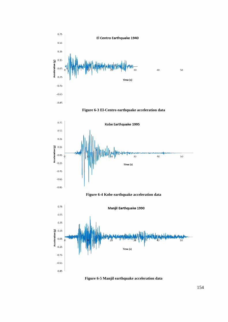
154
Figure 6-3 El-Centro earthquake acceleration data
Figure 6-4 Kobe earthquake acceleration data
Figure 6-5 Manjil earthquake acceleration data
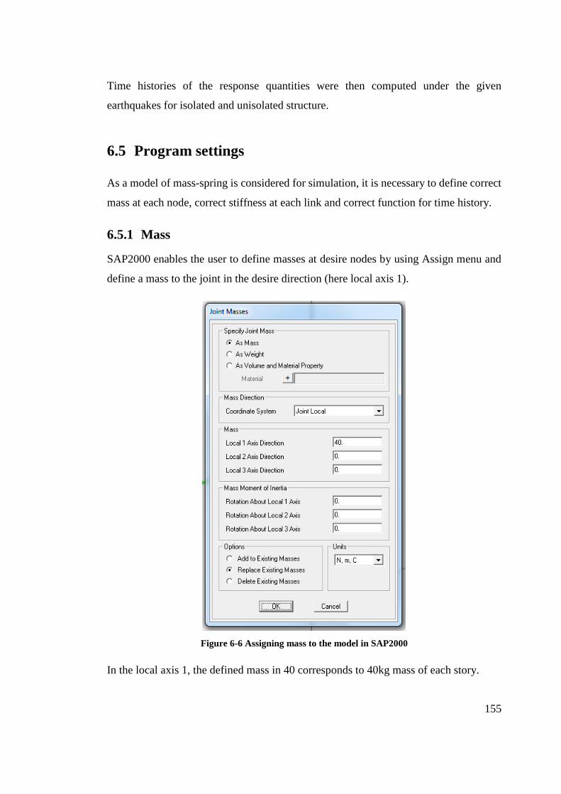
155
Time histories of the response quantities were then computed under the given
earthquakes for isolated and unisolated structure.
6.5 Program settings
As a model of mass-spring is considered for simulation, it is necessary to define correct
mass at each node, correct stiffness at each link and correct function for time history.
6.5.1 Mass
SAP2000 enables the user to define masses at desire nodes by using Assign menu and
define a mass to the joint in the desire direction (here local axis 1).
Figure 6-6 Assigning mass to the model in SAP2000
In the local axis 1, the defined mass in 40 corresponds to 40kg mass of each story.

156
6.5.2 Stiffness
In order to define the accurate stiffness to the model, it is necessary to draw the links
between each nodes. This is possible using Define menu where the option for defining
Links are available.
Figure 6-7 Defining lateral stiffness as Link in SAP2000
In the Link definition menu, SPR corresponds to lateral stiffness of each story and SPR-
B represents the lateral stiffness of the isolation system.
Figure 6-8 Definition of stiffness as Spring type Link in SAP2000

157
The mechanical properties of each Link can be defined by a Spring element as shown
in Figure 6-8. The value and direction of stiffness, then, is defined in the properties
menu as shown in Figure 6-9.
Figure 6-9 Definition of properties for spring links in SAP2000
The value of 469400 N/m corresponds to the lateral stiffness of each story is entered for
SPR element. Please note that, since the values for overall damping will be defined in
analysis settings the value for damping is considered as zero for this element here.
6.5.3 Time history input
For time-history inputs the user needs to first define the function of a quantity
(acceleration, displacement or force) over time. This is possible through Define menu
and sub-menu namely Function; where the user is able to introduce a time-history
records to the program. Time history records are text (*.txt) files format which in this
study are obtained from past earthquake records from USGS (United States Geological
Survey).

158
Figure 6-10 A sample of *.txt file corresponds to the earthquake recorded data
Figure 6-11 Definition of Kobe earthquake acceleration records as a function of time in SAP2000

159
Having known the sampling time for original record (which in this case is 0.02s) the
user is able to scale the time axis to the predefined target scale. The target scale for this
analysis was set to 0.316 for time, therefore, 0.00632 is entered as the intervals to the
program (Figure 6-11).
Upon defining the function of time history, it is necessary to assign it to a Load Case for
analysis by program. This is possible through Load Case Data setting from Define menu.
Figure 6-12 Load case data assignment to a time history function in SAP2000
As it is shown in Figure 6-12, the function is defined as acceleration with the scale factor
of 9.81 which denotes the gravity acceleration. Please note that, the recorded data used
for this analysis were acceleration readings by seismographs in unit of g. It should be
noted that the damping ratio is defined to the program at this step. The damping values
obtained from experiments are assigned to all modes of vibration here as 0.06 for fixed-
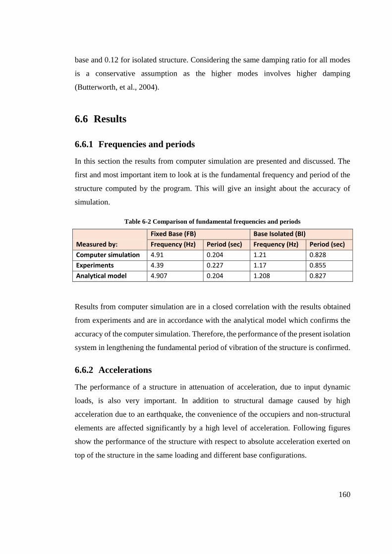
160
base and 0.12 for isolated structure. Considering the same damping ratio for all modes
is a conservative assumption as the higher modes involves higher damping
(Butterworth, et al., 2004).
6.6 Results
6.6.1 Frequencies and periods
In this section the results from computer simulation are presented and discussed. The
first and most important item to look at is the fundamental frequency and period of the
structure computed by the program. This will give an insight about the accuracy of
simulation.
Table 6-2 Comparison of fundamental frequencies and periods
Measured by:
Fixed Base (FB) Base Isolated (BI)
Frequency (Hz) Period (sec) Frequency (Hz) Period (sec)
Computer simulation 4.91 0.204 1.21 0.828
Experiments 4.39 0.227 1.17 0.855
Analytical model 4.907 0.204 1.208 0.827
Results from computer simulation are in a closed correlation with the results obtained
from experiments and are in accordance with the analytical model which confirms the
accuracy of the computer simulation. Therefore, the performance of the present isolation
system in lengthening the fundamental period of vibration of the structure is confirmed.
6.6.2 Accelerations
The performance of a structure in attenuation of acceleration, due to input dynamic
loads, is also very important. In addition to structural damage caused by high
acceleration due to an earthquake, the convenience of the occupiers and non-structural
elements are affected significantly by a high level of acceleration. Following figures
show the performance of the structure with respect to absolute acceleration exerted on
top of the structure in the same loading and different base configurations.

161
Figure 6-13 Acceleration response on top of the structure due to El-Centro earthquake (FB: Fixed
base and BI: Base isolated)
Figure 6-14 Acceleration response on top of the structure due to Kobe earthquake (FB: Fixed
base and BI: Base isolated)
Figure 6-15 Acceleration response on top of the structure due to Manjil earthquake (FB: Fixed
base and BI: Base isolated)

162
Table 6-3 Peak acceleration at each level of the structure due to input ground motion (m/s2)
MASSB 1st 2nd 3rd 4th 5th
ELCE
FB - 3.55466 6.04734 8.10146 10.20851 11.64578
BI 3.41102 3.50343 3.57001 3.60977 3.63773 3.6542
Reduction (%) 1.44 40.97 55.44 64.37 68.62
KOBE
FB - 6.47916 12.85764 17.44105 22.07453 24.91162
BI 8.08672 8.29152 8.44672 8.55902 8.63732 8.6815
Reduction (%) -27.97 34.31 50.93 60.87 65.15
MANJ
FB - 6.78363 9.98996 10.18468 8.59338 11.0826
BI 6.07364 6.1694 6.18779 6.19746 6.21461 6.23455
Reduction (%) 9.05 38.06 39.15 27.68 43.74
The response of the structure is drastically reduced when the present isolation system is
used. It is again confirmed that the present isolation system is able to reduce the level
of acceleration in the structure to a much lower level; more than 50% reduction is
observed on upper levels. It is observed that in a strong motion of Kobe, the acceleration
on first level is not reduced due to the use of isolation system. This, however, does not
have large effects as the value of peak acceleration at this level is low. It can be also
concluded that an acceptable level of performance for the isolation system corresponds
to all three cases of ground motion is observed. However, for Manjil ground motion
which involves a longer time oscillation, the ratio of attenuation is lower than shorter
oscillations such as El-Centro and Kobe.
6.6.3 Displacements
The other parameter which should be investigated is displacement in different levels of
the structure. Following figures correspond to the displacement response of the structure
with different base configurations and subject to three mentioned earthquakes.

163
Figure 6-16 Displacement response of the fixed-base structure due to El-Centro earthquake
Figure 6-17 Displacement response of the fixed-base structure due to Kobe earthquake
Figure 6-18 Displacement response of the fixed-base structure due to Manjil earthquake
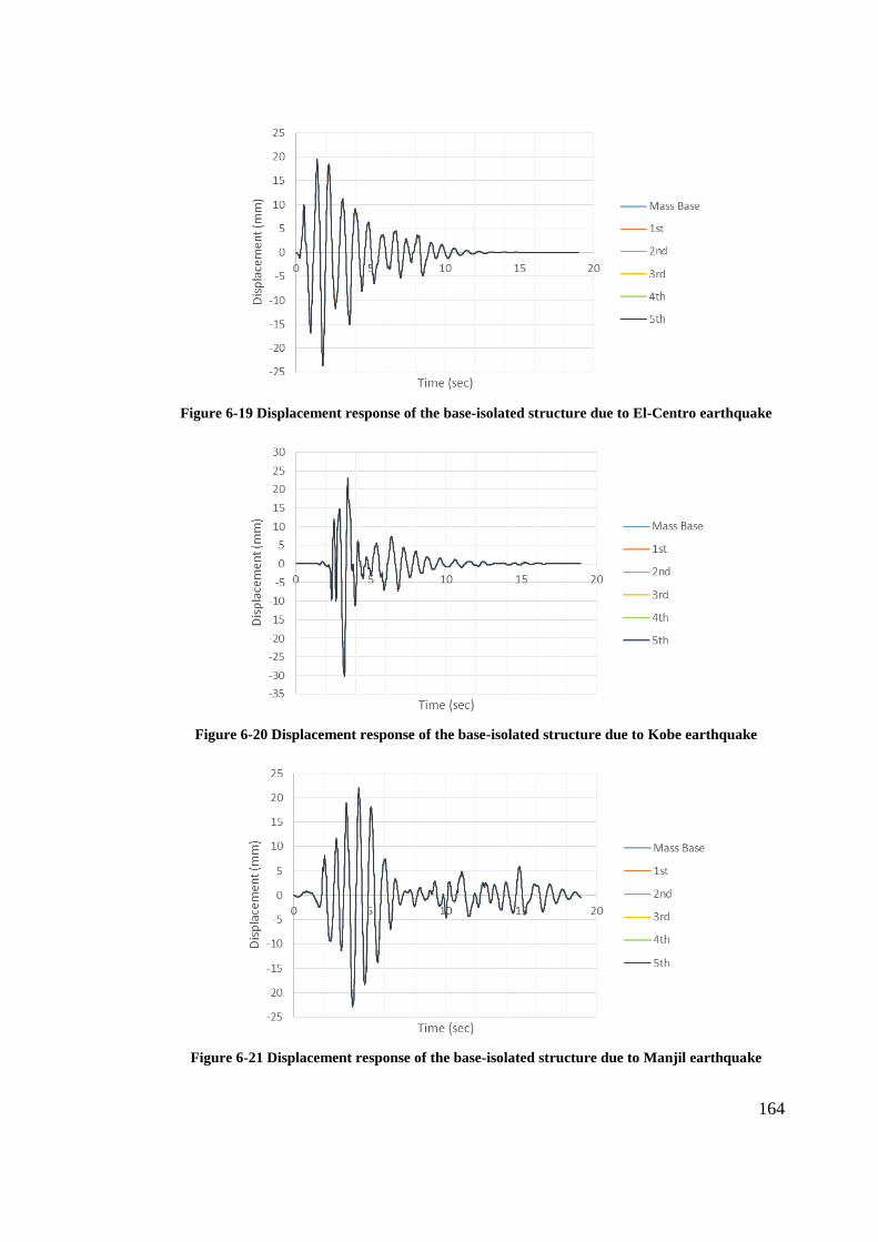
164
Figure 6-19 Displacement response of the base-isolated structure due to El-Centro earthquake
Figure 6-20 Displacement response of the base-isolated structure due to Kobe earthquake
Figure 6-21 Displacement response of the base-isolated structure due to Manjil earthquake

165
Table 6-4 Displacements and story drifts due to El-Centro earthquake (mm)
MASSB 1st 2nd 3rd 4th 5th
Fixed-Base
Displacement - 2.174 4.307 6.191 7.626 4.204
Story drift - - 2.133 1.884 1.435 3.422
Base-Isolated
Displacement 21.958 22.536 23.007 23.364 23.604 23.724
Story drift - 0.578 0.471 0.357 0.240 0.120
Table 6-5 Displacements and story drifts due to Kobe earthquake (mm)
MASSB 1st 2nd 3rd 4th 5th
Fixed-Base
Displacement - 5.921 11.354 15.909 19.252 10.552
Story drift - - 5.433 4.554 3.344 8.700
Base-Isolated
Displacement 28.110 28.829 29.397 29.815 30.090 30.226
Story drift - 0.719 0.568 0.418 0.275 0.136
Table 6-6 Displacements and story drifts due to Manjil earthquake (mm)
MASSB 1st 2nd 3rd 4th 5th
Fixed-Base
Displacement - 2.881 5.340 7.176 8.357 4.459
Story drift - - 2.459 1.836 1.181 3.898
Base-Isolated
Displacement 21.255 21.800 22.229 22.549 22.762 22.869
Story drift - 0.544 0.430 0.319 0.213 0.107
The isolated structure accommodates a large amount of displacement during the
earthquakes but the story drifts are reduced significantly in comparison to the unisolated
structure. The story drift known as one of the major causes of damage in structures
during earthquakes. Again, the appropriate performances of the present isolation system
under moderate and strong earthquakes are confirmed based on the displacement
response of the structure.
6.6.4 Base-shear
One of other important measures in earthquake engineering is the base-shear in a
structure due to an earthquake. The base-shear maximum values for fixed-base and base-
isolated structure subject to three mentioned earthquakes are presented in the following
table.

166
Table 6-7 Maximum base-shear force (N)
El-Centro Kobe Manjil
Fixed base 1020 2779 1352
Base isolated 318 407 308
Base-shear force is a horizontal load exerted to the structure basement at the time of
earthquake. A great reduction in base-shear is observed in the isolated structure.
6.6.5 Earthquake input energy
The performance of the present isolation system can be investigated with evaluating the
input energy to the structure due to the earthquakes (Figure 6-22 to Figure 6-27).
Table 6-8 Maximum input energy by different earthquakes (N-m)
El-Centro Kobe Manjil
Fixed base 15.40 97.45 20.80
Base isolated 11.07 29.38 13.77
A significant reduction in maximum input energy to the structure is observed when a
strong ground motion – Kobe – is considered. It can be concluded that the performance
of the isolation system in terms of reduction in the input energy is better when
considering strong earthquakes in comparison to moderate earthquakes.
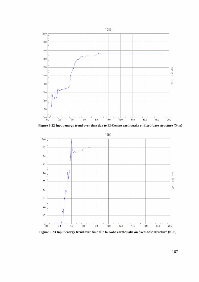
167
Figure 6-22 Input energy trend over time due to El-Centro earthquake on fixed-base structure (N-m)
Figure 6-23 Input energy trend over time due to Kobe earthquake on fixed-base structure (N-m)

168
Figure 6-24 Input energy trend over time due to Manjil earthquake on fixed-base structure (N-m)
Figure 6-25 Input energy trend over time due to El-Centro earthquake on base-isolated structure (N-m)

169
Figure 6-26 Input energy trend over time due to Kobe earthquake on base-isolated structure (N-m)
Figure 6-27 Input energy trend over time due to Manjil earthquake on base-isolated structure (N-m)

170
6.7 Conclusion
Numerical assessment of capability of the proposed isolation system was presented in
this chapter. The ability of the new system to protect structural and non-structural
elements from seismic hazards through its implementation on a structure were checked.
It is found that the new isolation system is able to greatly reduce the structure
accelerations, story drifts and base shears, while keeping acceptable displacement at
base. The proposed isolation system is highly effective when both moderate and strong
motion are considered.
It was clear from results that a larger period of vibration and a faster attenuation of
acceleration amplitude accompany the isolated structure. Although, the best
performance of the isolation system is obtained when strong motions are considered, the
results confirmed that the efficiency of the present system against earthquake attacks
does not highly depend on the type of input earthquake. It should be noted that, one of
the drawbacks of current base-isolation systems is dependency on the input shocks
characteristics.

171
7 Conclusion and future
works
This chapter concludes the thesis with a summary of results, the main contributions and
proposes topics that may be considered for future works.
7.1 Conclusion
Results from the experiments and numerical simulations reveal that the present isolation
system is a very efficient tool for seismic protection of building structures under
different earthquake features. The new isolation system exhibits a robust performance
for a scaled model of a typical five-story building. The behaviour of the structure
isolated by the new proposed system is relatively independent of the frequency content
and the amplitude of base excitation.
As the core of the idea for the new proposed isolation system was to make use of air-
bearing solutions, the air-bearing units were explicitly designed, analysed and optimised
through numerical simulation and further investigated through experimental tests. The
experimental tests on the air-bearing devices confirmed the best shape for the nozzles
of bearing in order to handle larger loads.
The purpose of the experimental study on the scaled structure was to determine whether
observations agree with or conflict with the predictions derived from the hypothesis
established earlier and its subsequent analytical model. The experiments confirmed that

172
the isolation system is able to lengthen the fundamental period of the structure and add
significant level of damping to the whole system (structure and its isolation). It was also
concluded that the isolation system reduces the level of acceleration exerted to the
structure subject to different applied impulse loadings. In addition, the isolation system
provides the structure with a reduction in the level of story drifts which is a known cause
of damages to the structures.
The computer investigation was conducted in order to simulate the behaviour of the
structure with two different base configurations (fixed base and base isolated) and
subject to different earthquakes; El-Centro 1940 as a moderate and short excitation,
Kobe 1994 as a strong and near-field ground motion, and Manjil 1990 as a strong ground
motion with long duration. The performance of the isolation system was confirmed
appropriate in terms of lengthening the fundamental period of vibration of the structure,
great attenuation of structural acceleration, significant reduction in story drifts and a
reduction of input energy to the structure in all cases. This is a great achievement that
the structure isolated by proposed isolation system is working quite independently from
the characteristics of input earthquake. As discussed in the literature review, one of the
drawbacks of current isolation systems is that they are not efficient in moderate
earthquakes and their performance is highly dependent on the input earthquake
characteristics; whereas, the new proposed system is able to protect a structure
regardless of the characteristics of the ground motion.
Measurements in engineering research works are usually accompanied by estimatipon
of their uncertainty. The value of the measured frequencies and periods by experiments
concur with the values obtained from the analytical model and numerical simulations.
There are only around 10% and 3% differences for fixed-base structure and base-
isolated structure, respectively, between experiments and computer modelling. This
stems from the uncertainty in the stiffness and damping characteristics of the structure
and its isolation system. A small variation in stiffness produces quite a large difference
in measures of dynamic parameters.
There are some limitations in computing equivalent damping values using experimental
data which arises because linear behaviour for a dynamic system is normally assumed.

173
When the given dynamic system is behaving highly nonlinear, a substantial error could
be introduced into the damping estimation. Nonetheless, it is routine to assume linear
viscous damping in experimental data analysis.
7.2 Contributions
This research aimed to develop an innovative isolation system that is efficient and has
some particular capabilities which are not offered by contemporary isolation systems.
The proposed isolation system works as a semi-active isolation system which can be
triggered by the signals received from metrological centres as an early warning. The
isolation system, then, employs air-bearing solutions to decouple the super-structure
from its base at the time of ground motion. The air-bearing system is accompanied by a
re-centring mechanism such as rubber-bearings or friction pendulum for self-re-
centring. As the horizontal stiffness at the base of a structure is reduced the fundamental
period of the structure is shifted to a greater one and the accelerations exerted in the
structure are reduced. Below is the list of features provided by the new system:
Great decoupling system
Lengthening the vibration period to the designer desire
Involving a wide range of base stiffness
Great level of energy dissipation
Self-re-centring system
Suitable for all range of earthquake from moderate to strong motions
Improvement of damping mechanism
7.3 Future works
Further research beyond the scope of this study is recommended in relation to the present
isolation system in the following area:

174
Testing the scaled structure with and without the proposed isolation system on a
shaking table in order to observe the behaviour of the structure and performance
of the isolation system in practice.
Checking the feasibility of the proposed isolation system for bridges isolation.
Design and development of a large-scale prototype, for characterisation
evaluations and experimental tests.
Undertaking a cost analysis of the isolation system with respect to the savings in
the use of materials and energy from production to construction and
implementation.
Checking the uplift response of the structure when isolated with the proposed
isolation system and subjected to different kinds of earthquakes.
Checking the influence of the proposed isolation system on torsional responses.
Performing a comparative study on the proposed system against current isolation
systems.
Performing a numerical investigation on the proposed air-bearing with dynamic
mesh generation.
Future works are not limited to the above mentioned activities and researchers interested
in this area may define their own aims and objectives to fill the gap in knowledge.
175
8 References
Ab-Malek, K. & Kamaruddin, S., 2010. Opportunities Of Manufacturing Engineering
Rubber Products. Buloh, Rubber research institute of Malaysia.
Aerogo, 2015. moving heavy loads up to 5000 tons. [Online]
Available at: http://www.aerogo.com/heavy-load-moving/moving-heavy-loads-up-to-
5000-tons/4
[Accessed 10 08 2015].
Airfloat, 2015. casestudy. [Online]
Available at: http://www.airfloat.com/casestudy/arena-seating/
[Accessed 10 08 2015].
ANSYS, 2015. ANSYS help. Canonsburg: ANSYS.
Aris, R., 1989. Vectors, Tensors and the Basic Equations of Fuid Mechanics. Newyork:
Dover Publications.
Avitabile, P., 2001. Experimental Modal Analysis , Lowell: University of Massachusetts
Lowell.
Bailey, W. S., 1961. Gas Particle Flow in an Axisymmetric Nozzle. ARS Journal, 31(6),
pp. 793-798.
Bernstein, A., Heiser, W. H. & Hevenor, C., 1967. Compound-Compressible Nozzle
Flow. Journal of Applied Mechanics, 34(3), pp. 548-554.

176
Beychok, M., 2010. De Laval nozzle. [Online]
Available at: http://en.citizendium.org/wiki/File:De_Laval_nozzle_2.png
[Accessed 22 09 2015].
Boroschek, K. R., 2002. Base Isolation in Hospitals. Barbados, Seminar on Design of
Health Facilities to Resist Natural Hazards .
Braga, F., 2001. Seismic Isolation Using Slide and Rubber Bearings. Assisi, Italy, s.n.
Brennan, D., 2001. The numerical simulation of two phase flows in settling tanks.
London: Imperial College London.
Buchanan, A. et al., 2011. Base Isolation and Damage Resistant Technologies for
Improved Seismic Performance of Buildings, Christchurch: University of Canterbury.
Buckle, I. G., 2000. Passive Control of Structures for Seismic Loads. s.l., s.n.
Butterworth, J., Lee, J. H. & Davidson, B., 2004. Experimental Determination of Modal
Damping from Full Scale Testing. Vancouver, 13th Conference on Earthquake
Engineering .
Castillo, J., 1991. Discrete Variational Grid Generation. In: J. Castillo, ed.
MATHEMATICAL ASPECTS OF NUMERICAL GRID GENERATION. s.l.:SIAM.
Chopra, 2007. Dynamics of Structures. Third Edition ed. Upper Saddle River: Pearson
Prentice Hall.
Clancy, L., 1975. Aerodynamics. New York: John Wiley & Sons Inc.
Clough, R. W. & Penzien, J., 2003. DYNAMICS OF STRUCTURES. 3rd ed. Berkeley:
Computers & Structures.
Cooperstock, F., 2009. General relativistic dynamics: extending Einstein's legacy
throughout the univese. Singapore: World Scientific.
De Silva, C. W., 2007. Vibration Damping, Control, And Design. Boca Raton: Taylor
& Francis.

177
Deardorff, W., 1970. numerical study of three-dimensional turbulent channel °ow at
large Reynolds numbers. Journal of Fluid Mechanics, 41(2), p. 453{480.
Elarms, 2012. Earthquake Alarm System. [Online]
Available at: www.elarms.org
[Accessed 1st March 2012].
Eswaran, V. & Pope, S., 1988. Direct numerical simulations of the turbulent mixing of
a passive scalar. Physics of Fluids, 31(March), pp. 506-520.
Eurocode8, 2011. Design of structures for earthquake resistance Prt 1, s.l.: British
standard.
Forni, M. & Martelli, A., 1998. Seismic isolation of civil buildings in europe. Progress
in Structural Engineering and Materials, Volume Voll(3), pp. 286-294.
Forni, M. & Martelli, A., 1998. Seismic isolation of civil buildings in europe. Progress
in Structural Engineering and Materials, Volume Voll(3), pp. 286-294.
Fujita, S., Minagawa, K., b, G. & HaruoShimosaka, 2011. Intelligent seismic isolation
system using air bearings and earthquake early warning. Soil Dynamics and Earthquake
Engineering, 31(2), p. 223–230.
GeoSIG, 2013. AC-43 Force Balance Accelerometer, Schlieren: GeoSIG.
GeoSIG, 2015. GMSplus Measuring System, Schlieren: GeoSIG.
Godfrey-Smith, P., 2003. Theory and Reality: An introduction to the philosophy of
science. Chicago: University of Chicago Press.
Griffith, T., 2001. The physics of everyday phenomena: a conceptual introduction to
physics. 3rd ed. Boston: McGraw-Hill.
Harris, F., 1978. On the use of windows for harmonic analysis with the discrete Fourier
Transform. Proc. IEEE, 66(January), pp. 51-83.
Hendriks, F., 2001. Shape optimization of pressurized air bearings, Hawthorne:
Rensselaer Polytechnic Institute.

178
Hibbeler, R. C., 2002. Engineering Mechanics Dynamics. 2nd ed. Singapore: Prentice
Hall.
HOVAIR, 2013. How does an air bearing work?. [Online]
Available at: http://hovair.com/information-files/what-is-an-air-bearing-how-does-an-
air-bearing-work.htm
[Accessed 01 06 2013].
Iqbal, A., 2006. Soft First Story with Seismic Isolation System. s.l., NZSEE Conference.
Ismail, M., 2009. An Innovative Isolation Device for Aseismic Design. PhD Thesis ed.
Barcelona: Technical University of Catalonia.
Ismail, M., Rodellar, F. & Ikhouane, 2010. An innovative isolation device for aseismic
design. Engineering Structures, pp. 1168-1183.
Izumi, M., 1988. State-of-the-art report: Base isolation and passive seismic response
control. Tokyo, s.n., pp. 385-396.
Izumi, M., 1988. State-of-the-art report: Base isolation and passive seismic response
control. Tokyo, s.n., pp. 385-396.
Jangid, R. S., 1996. Optimum Damping in Non-linear Base Isolation System. Journal
of Sound and Vibration , 189(4), pp. 477-487.
Jasak, H., 1996. Error Analysis and Estimation for the Finite Volume Method with
Applications to Fluid Flows. London: Imperial College of Science, Technology and
Medicine.
Jevons, W. S., 1958. The Principles of Science: A Treatise on Logic and Scientific
Method. New York: Dover Publications.
Kani, N., Takayama, M. & Wada, A., 2006. Performance of Seismically Isolated
Buildings in Japan. San Francisco, 8th U.S. National Conference on Earthquake
Engineering .
179
Kelly, T. E., 2001. Base Isolation of Structures, Wellington: Holmes Consulting Group
Ltd.
Kravchuk, N., Colquhoun, R. & Porbaha, A., 2008. Development of a Friction
Pendulum Bearing Base Isolation System for Earthquake Engineering Education.
Sacramento, American Society for Engineering Education Pacific Southwest Annual.
Kuramoto, H., 2006. Seismic Design Codes for Buildings in Japan. Journal of Disaster
Research.
Marsico, M. R., 2008. Seismic Isolation and Energy Dissipation: Theoretical Basis and
Applications. Napoli: Napoli Federico II university.
MATLAB help (2011) The MathWork Inc.
Mavriplis, D. J., 1996. Mesh generation and adaptivity for complex geometries and
flows. In: R. Peyret, ed. Handbook of computational fluid mechanics / edited by Roger
Peyret. 2 ed. London: Academic Press.
Monfared, H., Shirvani, A. & Nwaubani, S., 2013. An investigation into the seismic
base isolation from practical perspective. INTERNATIONAL JOURNAL OF CIVIL AND
STRUCTURAL ENGINEERING, 3(3), pp. 451- 463.
Mukai, T., 2006. Analysis of Dynamic Characteristics of Air Bearing, s.l.: NIPPON
STEEL.
Naeim, F. & Kelly, J. M., 1999. Design of seismic isolated structures: from theory to
practice. New York: John Wiley & Sons.
Naeim, F. & Kelly, J. M., 1999. Design of seismic isolated structures: from theory to
practice. New York: John Wiley & Sons.
Naeim, F. & Kelly, J. M., 1999. Design of seismic isolated structures: from theory to
practice. New York: John Wiley & Sons.

180
Nakashima, M. & Chusilp, P., 2003. A Partial View of Japanese Post-Kobe Seismic
Design and Construction Practices. Earthquake Engineering and Engineering
Seismology, Vol. 4, No. 1.
Newway, 2006. Air Bearing Aplication and Design Guide, Aston: New way air bearing.
Ørsted, H. C., 1998. Selected Scientific Works of Hans Christian Ørsted. Princeton:
Princeton University Press.
Parducci, A., 2010. SEISMIC ISOLATION: WHY, WHERE, WHEN, San Francisco:
esempi di Architettura.
Percision, N. W., 2003. Air Bearing Application and Design Guid, Aston, PA: New
Way Percision.
Popper, K., 2002. Conjectures and Refutations: The Growth of Scientific Knowledge.
Abingdon: Routledge Classics.
Popper, K., 2002. The Logic of Scientific Discovery. London: Routledge Classics.
Powell, J. W., 1970. Design of Aerostatic Bearings. s.l.:Machinery Publishing Ltd .
Ramezanpour, A., 2009. AUTHENTIC OPTIMISATION STUDY OF THE NOVEL
COMPACT HEAT EXCHANGER. 1st ed. s.l.:VDM Verlag.
Ramirez, R., 1975. The FFT: Fundamentals and concepts, Beaverton: Tekronix.
Renn, J.-C. & Hsiao, C.-H., 2004. Experimental and CFD study on the mass flow-rate
characteristic of gas through orifice-type restrictor in aerostatic bearings. Tribology
International, 37(4), pp. 309-315.
Roussis, P. C. & Constantinou, M. C., 2006. Uplift-restraining Friction Pendulum
seismic isolation system. EARTHQUAKE ENGINEERING AND STRUCTURAL
DYNAMICS, 35(5), p. 577–593.
Saiful-Islam, Jumaat, M. J. & Zamin, M., 2011. Seismic isolation in buildings to be a
practical reality:Behavior of structure and installation technique. Journal of Engineering
and Technology Research, Vol. 3(4),, pp. pp. 99-117.

181
Solving, 2015. 400t handling system for diesel engines. [Online]
Available at: http://www.solving.com/case-studies/400t-handling-system-for-diesel-
engines
[Accessed 10 08 2015].
Sterken, C., 2003. Jean Baptiste Joseph Fourier. San Francisco, Astronomical Society
of the Pacific.
Symans, M. D., 2004. Seismic Protective Systems. s.l.:FEMA 451.
Tajirian, F. F., 1998. Base Isolation Design for Civil Components and Civil Structures.
San Francisco, Structural Engineers World Congress.
Tiwari, P., Stein, A. & Lin, Y.-L., 2013. Dual-Solution and Choked Flow Treatment in
a Streamline Curvature Throughflow Solver. Journal of Turbomachinery, 135(4), p.
041004.
USGS, 2015. Earthquake Early Warning. [Online]
Available at: http://earthquake.usgs.gov/research/earlywarning/
[Accessed 20 10 2015].
Walters, M., 2003. THE SEISMIC RETROFIT OF THE OAKLAND CITY HALL. San
Francisco , SMIP03 Seminar on Utilization of Strong-Motion Data.
Wei, L. & Gang, B., 2010. Entrance Effect on Load Capacity of Orifice Compensated
Aerostatic Bearing with Feeding Pocket. CHINESE JOURNAL OF MECHANICAL
ENGINEERING, Volume 23.
Wilcox, D. C., 2006. Turbulence Modeling for CFD. 3rd ed. La Canada, California:
DCW Industries, Inc.
Wilczek, F. & Devine, B., 2006. Fantastic realities : 49 mind journeys and a trip to
Stockholm. New Jersey: World Scientific.
Wright, K. R. & Zegarra, A. V., 2000. Machu Picchu: A Civil Engineering Marvel.
s.l.:ASCE Press.

182
Wu, Y. M. & Samali, B., 2002. Shake Table Testing of a Base Isolated Model.
Engineering Structure, 24(2002), pp. 1203-1215.
Zhou, F. L., Yang, Z., Liu, W. G. & Tan, P., 2004. New Seismic Isolation System For
Irregular Structure With The Largest Isolation Building Area In The World. Vancouver,
13th World Conference on Earthquake Engineering.

183
Appendices
A.1 Research flowchart
Diagram below shows the research path from proposal to thesis.

184
A.2 BI projects around the world
Seismic base-isolation projects in U.S.A
Project Purpose and
location
Isolating
system
Construction
completed in
year
Description
Foothill Communities
Law and Justice Center
(Naeim & Kelly, 1999)
Official building
to be built, Rancho
Cucamonga near
Los Angeles
Isolation bearing,
98 High-damping
natural rubbers
1985 The first base-
isolated building in
the United States and
the first building in
the world to use
High-damping
natural rubber, the
four stories high with
170,000 ft2 area,
designed to withstand
an 8.3 magnitude
earthquake.
Flight simulator
manufacturing facility
(Naeim & Kelly, 1999)
Official building
to be built, Salt
Lake city
Isolation bearing,
98 isolators, 50 of
the bearings are
lead plug and 48
plain elastomeric
bearings
1988 The building is
located very close to
the Wastach Fault
which has capability
of generating 7.5
magnitude
earthquakes, a four-
story building with
116,000 ft2 area.
The M. L. King/C. R.
Drew Diagnostic
trauma center (Naeim
& Kelly, 1999)
Hospital building
to be built ,
Willowbrook, Los
Angeles county
Isolation and
Sliding bearings,
70 high-damping
natural rubbers
and 12 sliding
bearings
1995 The largest isolation
bearings fabricated in
the United States at
the time, a five stories
building with
140,000 ft2 area.
AutoZone head quarter
(Naeim & Kelly, 1999)
Official building
to be built,
Memphis
Isolation bearing,
composed of 24
lead-plug rubber
isolators and 19
high-damping
1995 A large office
building, eight stories
and 250,000 ft2 area,
withstand a
maximum seismic
event of 9.0

185
natural rubber
isolators
magnitude, without
the base isolation
system, the building
itself could withstand
a magnitude 6.0
event.
Oakland City Hall
(Walters, 2003)
Historical building
to be retrofitted,
Oakland
Isolation bearing,
composed of 113
elastomeric
bearings
approximately half
of which have
lead cores
1995 The top of the 18-
story building is 324
feet above street level
which was completed
in 1914, the
first high-rise
government building
in the United States at
the time.
U.S. Court of Appeals
(Naeim & Kelly, 1999)
(Kravchuk, et al.,
2008)
Historical building
to be retrofitted,
San Francisco
Friction Pendulum
System, 256
bearings
1996 A five-story building
with 350,000 ft2 area.
was built in 1905 on a
steel gravity frame
with unreinforced
granite and brick
masonry walls.
San Francisco City
Hall (Naeim & Kelly,
1999)
Historical building
to be retrofitted,
San Francisco
Isolation bearing,
composed of 530
lead-plug rubber
bearings
1998 A five-story building
with 300 ft high
dome. The structural
system is a steel
frame which was
designed in 1912.
San Francisco
International Airport
(International
Terminal) (Kravchuk,
et al., 2008)
Building to be
built, San
Francisco,
California
Friction Pendulum
System, 267
bearings
2000 The largest isolated
building of the world,
can resist a
magnitude 8
earthquake.

186
Some seismic base-isolation projects in Japan
Project Purpose and
location
Isolating
system
Construction
completed in
year
Description
Science University
of Tokyo (Izumi,
1988)
Official building to
be built, Tokyo
Double columns
and dampers
1981 The first modern base-
isolated building in
Japan
Yachiyodai Unitika
(Izumi, 1988)
Residential
building to be built,
Tokyo
Laminated rubber
bearing and PC
plate friction
damper
1983 -
Oyles Technical
center (Izumi,
1988)
Official Building
to be built,
Laminated lead
rubber bearing, 45
bearings
1987 -
West Japan Postal
Computer Center
(Naeim & Kelly,
1999)
Official building to
be built, Sanda
120 elastomeric
Isolators,
additional steel and
lead dampers
Before 1995 A six-story building,
506,000 ft2 area, has
shown a very
reasonable
performance during the
1995 Kobe earthquake
C-1 Building Computer center to
be built, Fuchu
City, Tokyo
68 Lead Rubber
Bearing
1992 A seven-story building,
with the area of
407,350 ft2
Maiya Matsumoto
hospital
(Boroschek, 2002)
Hospital to be built,
Kyoto
24 rubber bearings,
8 lead dampers and
14 steel bar
dampers
1997 -
Kyorin University
School of Medicine
(Boroschek, 2002)
Hospital to be built,
Shinkawa, Mitaka
City, Tokyo
72 lead rubber
bearings
2000 A seven-story building,
one below ground, with
maximum height of
40.30m
NS computer center
(Kani, et al., 2006)
Official building to
be built, Nagaoka
City
- 2004 The first data center
with seismic isolation

187
Some notable seismic base-isolation projects around the world
Project Purpose and
location
Isolating
system
Construction
completed in
year
Description
New Fire Station and
Headquarter of Napoli
(Forni & Martelli,
1998)
Official building,
Italy
Mechanical
dissipaters and
isolators
1981 The first base-isolated
building in Italy
Union House
Auckland (Naeim &
Kelly, 1999)
Official building,
Auckland, New
Zealand
Sleeved-pile
system
1984 A 12-story reinforced
concrete building
with additional
damping system
Ancona SIP buildings
(Marsico, 2008)
(Naeim & Kelly, 1999)
(Forni & Martelli,
1998)
Official building,
Italy
Rubber bearings
with recessed
plate connections
1988-1992 The first base-isolated
building in Italy with
application of rubber
bearings
Wellington Central
Police Station (Naeim
& Kelly, 1999)
Official building,
Wellington, New
Zealand
Sleeved-pile
system
1991 A 10-story reinforced
concrete building
with additional lead-
extrusion dampers for
controlling purposes
National museum of
New Zealand (Braga,
2001) (Naeim & Kelly,
1999)
Museum,
Wellington, New
Zealand
142 lead-rubber
bearings, and 36
Teflon pads under
the shear walls
1995 A five story building
with 23m high
Department of
Mathematics,
University of
Basilicata (Forni &
Martelli, 1998)
Official Building,
Italy
89 High-damping
Rubber bearings
1995 Block 1-4 of Faculty
of Agriculture also
were built on 132
bearings in the same
year
Museum (Zhou, et al.,
2004)
Official building to
be built, China
Rubber bearings 1996 A 13-story reinforced
concrete building
New Zealand
parliament House
(Naeim & Kelly, 1999)
Historical building
to be retrofitted,
Wellington, New
Zealand
More than 514
lead-rubber
bearings
1996 The building was
designed in 1911 and
strengthened and
refurbished between
1991 to 1996

188
Corinth Canal Bridges
(Roussis &
Constantinou, 2006)
Bridge to be built,
Greece
Elastomeric and
Flat sliding
bearings
1997 One of the notable
seismic-isolation in
Greece
LNG Tanks, In-Chon
(Tajirian, 1998)
Infrastructure,
Korea
Steel-laminated
rubber bearings
1997 An example of
utilizing base-
isolation system for
infrastructures
Sanctuary of Siracusa
(Marsico, 2008)
Temple to be
retrofitted, Italy
New kind
bearings namely
“moon’s sickle”
2006 One of the notable
retrofitting projects in
Europe
Parand residential
project (Ab-Malek &
Kamaruddin, 2010)
Residential
buildings to be
built, Iran
More than 8,000
rubber bearings
Under
construction
150 blocks of
residential building of
8 and 12-storey high,
this is the world’s
largest application of
seismic rubber
bearings in a single
project, 360rubber
bearings had been
installed until 2009

189
A.3 Roller bearing specifications
Part number 9101 was chosen and used with respect to space restrictions under the
scaled structure and roller’s load capacity.

190

191
A.4 Modal analysis (fixed-base model)
M= structural mass matrix
K= structural lateral stiffness matrix
M
40
0
0
0
0
0
40
0
0
0
0
0
40
0
0
0
0
0
40
0
0
0
0
0
40
K
469400
469400
0
0
0
469400
938800
469400
0
0
0
469400
938800
469400
0
0
0
469400
938800
469400
0
0
0
469400
938800
M1
0.025
0
0
0
0
0
0.025
0
0
0
0
0
0.025
0
0
0
0
0
0.025
0
0
0
0
0
0.025
MT
40
0
0
0
0
0
40
0
0
0
0
0
40
0
0
0
0
0
40
0
0
0
0
0
40
D M1
K
1.173 104
1.173 104
0
0
0
1.173 104
2.347 104
1.173 104
0
0
0
1.173 104
2.347 104
1.173 104
0
0
0
1.173 104
2.347 104
1.173 104
0
0
0
1.173 104
2.347 104
eigenvals D( )
950.7
8.1 103
2.013 104
3.322 104
4.321 104
eigenvecs D "R"( )[ ]
0.597
0.549
0.456
0.326
0.17
0.549
0.17
0.326
0.597
0.456
0.456
0.326
0.549
0.17
0.597
0.326
0.597
0.17
0.456
0.549
0.17
0.456
0.597
0.549
0.326
mode1
0
0.17
0.326
0.456
0.549
0.597
mode2
0
0.456
0.597
0.326
0.17
0.549
mode3
0
0.597
0.17
0.549
0.326
0.456
mode4
0
0.549
0.456
0.17
0.597
0.326
mode5
0
0.326
0.549
0.597
0.456
0.17

192
0 0.2 0.4 0.60
1
2
3
4
5
stories
mode1
1 0.5 0 0.5 10
1
2
3
4
5
stories
mode3
1 0.5 0 0.5 10
1
2
3
4
5
stories
mode2
0.5 0 0.5 10
1
2
3
4
5
stories
mode4
1 0.5 0 0.5 10
1
2
3
4
5
stories
mode5
0.597
0.549
0.456
0.326
0.17
0.549
0.17
0.326
0.597
0.456
0.456
0.326
0.549
0.17
0.597
0.326
0.597
0.17
0.456
0.549
0.17
0.456
0.597
0.549
0.326
T
0.597
0.549
0.456
0.326
0.17
0.549
0.17
0.326
0.597
0.456
0.456
0.326
0.549
0.17
0.597
0.326
0.597
0.17
0.456
0.549
0.17
0.456
0.597
0.549
0.326
eigenvals D( )
950.7
8.1 103
2.013 104
3.322 104
4.321 104
i 1 5
i
950.7
38.1·10
42.013·10
43.322·10
44.321·10
i
i
...
i
30.833
90.002
141.88
182.263
207.88
fi
i
2
fi
4.907
14.324
22.581
29.008
33.085
Ti
1
fi
Ti
0.204
0.07
0.044
0.034
0.03

193
m T
M
40
1.066 1014
3.553 1015
0
1.021 1014
9.326 1015
40
0
0
1.599 1014
3.553 1015
3.553 1015
40
1.243 1014
0
1.332 1015
1.776 1015
1.243 1014
40
7.994 1015
1.066 1014
1.599 1014
0
6.217 1015
40
i 1 5
mi i
40
40
40
40
40
r
1
1
1
1
1
L T
M r
83.882
26.409
13.919
7.751
3.541
Li 1
83.882
-26.409
13.919
7.751
3.541
i
Li 1
mi i
...
i
2.097
-0.66
0.348
0.194
0.089
meffi
Li 1
2
mi i
...
meffi
175.906
17.435
4.843
1.502
0.314
mtotal meff 200

194
A.5 Modal analysis (base isolated)
M= structural mass matrix
K= structural lateral stiffness matrix
M
40
0
0
0
0
0
0
40
0
0
0
0
0
0
40
0
0
0
0
0
0
40
0
0
0
0
0
0
40
0
0
0
0
0
0
40
K
469400
469400
0
0
0
0
469400
938800
469400
0
0
0
0
469400
938800
469400
0
0
0
0
469400
938800
469400
0
0
0
0
469400
938800
469400
0
0
0
0
469400
483900
M1
0.025
0
0
0
0
0
0
0.025
0
0
0
0
0
0
0.025
0
0
0
0
0
0
0.025
0
0
0
0
0
0
0.025
0
0
0
0
0
0
0.025
D M1
K
1.173 104
1.173 104
0
0
0
0
1.173 104
2.347 104
1.173 104
0
0
0
0
1.173 104
2.347 104
1.173 104
0
0
0
0
1.173 104
2.347 104
1.173 104
0
0
0
0
1.173 104
2.347 104
1.173 104
0
0
0
0
1.173 104
1.21 104
eigenvals D( )
57.654
3.258 103
1.183 104
2.353 104
3.524 104
4.38 104
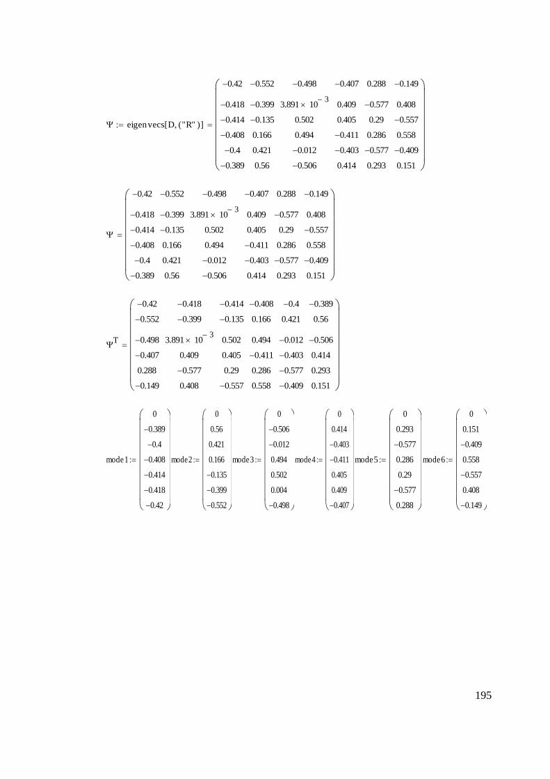
195
eigenvecs D "R"( )[ ]
0.42
0.418
0.414
0.408
0.4
0.389
0.552
0.399
0.135
0.166
0.421
0.56
0.498
3.891 103
0.502
0.494
0.012
0.506
0.407
0.409
0.405
0.411
0.403
0.414
0.288
0.577
0.29
0.286
0.577
0.293
0.149
0.408
0.557
0.558
0.409
0.151
0.42
0.418
0.414
0.408
0.4
0.389
0.552
0.399
0.135
0.166
0.421
0.56
0.498
3.891 103
0.502
0.494
0.012
0.506
0.407
0.409
0.405
0.411
0.403
0.414
0.288
0.577
0.29
0.286
0.577
0.293
0.149
0.408
0.557
0.558
0.409
0.151
T
0.42
0.552
0.498
0.407
0.288
0.149
0.418
0.399
3.891 103
0.409
0.577
0.408
0.414
0.135
0.502
0.405
0.29
0.557
0.408
0.166
0.494
0.411
0.286
0.558
0.4
0.421
0.012
0.403
0.577
0.409
0.389
0.56
0.506
0.414
0.293
0.151
mode1
0
0.389
0.4
0.408
0.414
0.418
0.42
mode2
0
0.56
0.421
0.166
0.135
0.399
0.552
mode3
0
0.506
0.012
0.494
0.502
0.004
0.498
mode4
0
0.414
0.403
0.411
0.405
0.409
0.407
mode5
0
0.293
0.577
0.286
0.29
0.577
0.288
mode6
0
0.151
0.409
0.558
0.557
0.408
0.149

196
0.5 0.4 0.3 0.2 0.1 00
2
4
6
stories
mode1
1 0.5 0 0.5 10
2
4
6
stories
mode2
1 0.5 0 0.5 10
2
4
6
stories
mode3
0.6 0.2 0.2 0.60
2
4
6
stories
mode4
0.6 0.4 0.2 0 0.2 0.40
2
4
6
stories
mode5
1 0.5 0 0.5 10
2
4
6
stories
mode6
i 1 6
eigenvals D( )
57.654
3.258 103
1.183 104
2.353 104
3.524 104
4.38 104
i
57.654
33.258·10
41.183·10
42.353·10
43.524·10
44.38·10
i
i
...
i
7.593
57.075
108.75
153.399
187.712
209.294
fi
i
2
fi
1.208
9.084
17.308
24.414
29.875
33.31
Ti
1
fi
Ti
0.827
0.11
0.058
0.041
0.033
0.03

197
m T
M
40
3.553 1015
6.217 1015
8.882 1015
0
7.55 1015
7.105 1015
40
7.105 1015
0
1.776 1015
7.105 1015
8.882 1015
7.105 1015
40
8.882 1015
4.441 1015
3.553 1015
9.77 1015
0
5.329 1015
40
1.776 1015
0
1.776 1015
4.441 1015
4.441 1015
4.441 1015
40
7.994 1015
5.329 1015
6.217 1015
3.553 1015
0
9.548 1015
40
i 1 6
mi i
40
40
40
40
40
40
r
1
1
1
1
1
1
L T
M r
97.946
2.491
0.62
0.255
0.12
0.05
Li 1
-97.946
2.491
-0.62
0.255
0.12
0.05
i
Li 1
mi i
...
i
-2.449
0.062
-0.015
-36.37·10
-33.01·10
-31.253·10
meffi
Li 1
2
mi i
...
meffi
239.833
0.155
-39.61·10
-31.623·10
-43.623·10
-56.285·10
mtotal meff 240

198
A.6 Air pump specifications
1- The air pump model used for producing pressurised air:

199
2- The air pump specifications according to its provider’s manual:
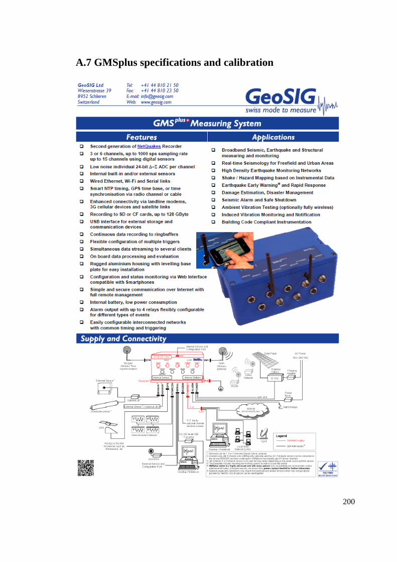
200
A.7 GMSplus specifications and calibration

201

202

203

204
A.8 Accelerometer specifications and calibration

205

206

207

208
A.9 FFT algorithm and implementation
The functions Y = fft(x) and y = ifft(X) implement the transform and inverse transform
pair given for vectors of length N by:
where
is an Nth root of unity.
Y = fft(x) returns the discrete Fourier transform (DFT) of vector x, computed with a fast
Fourier transform (FFT) algorithm.
Y = fft(X,n) returns the n-point DFT. fft(X) is equivalent to fft(X, n) where n is the size
of X in the first nonsingleton dimension. If the length of X is less than n, X is padded
with trailing zeros to length n (MATLAB help, 2011).
MATLAB implementation code for FFT analysis:
Fs = 50; % Sampling frequency T = 1/Fs; % Sample time L = 1000; % Length of signal t = (0:L-1)*T; % Time vector NFFT = 2^nextpow2(L); % Next power of 2 from length of y data1=transpose(xFBDispl); data1(isnan(data1))=[]; data2=transpose(xBIDispl); data2(isnan(data2))=[]; Y1= fft(data1,NFFT)/L; Y2 = fft(data2,NFFT)/L; f = Fs/2*linspace(0,1,NFFT/2+1); % Plot single-sided amplitude spectrum. plot(f,2*abs(Y1(1:NFFT/2+1))) title('Single-Sided Amplitude Spectrum of y(t)') xlabel('Frequency (Hz)') ylabel('|Y(f)|') hold on plot(f,2*abs(Y2(1:NFFT/2+1)),'r')

209

![SEISMIC ROOF ISOLATION OF HALKAPINAR … · most efficient seismic isolation solution for the Halkapınar Gymnasium. In this thesis, theory of seismic isolation, ... [18] (From AASHTO](https://img.dokumen.tips/doc/110x75/5b5ba6ce7f8b9a905c8e7903/seismic-roof-isolation-of-halkapinar-most-efficient-seismic-isolation-solution.jpg)