Embed Size (px)
Citation preview

A Neighborhood Search Algorithm for the Capacitated
Minimum Spanning Tree Problem Authors Dr Jun Han Associate Professor of Computing Science Email: [email protected] Phone: +86 10 8231 6340 Fax: +86 10 8231 6796 Post: Mailbox 7-28
Beihang University Beijing 100083, P.R.China
Dr Stephen Sugden Associate Professor of Mathematics Email: [email protected] Phone: +61 7 5595 3325 Fax: +61 7 5595 3320 Post: School of Information Technology Bond University Gold Coast, QLD 4229, Australia Dr Jinpeng Huai Professor of Computer Science Email: [email protected] Phone: +86 10 8231 4838 Fax: +86 10 8232 8058 Post: Mailbox 7-28
Beihang University Beijing 100083, P.R.China
Zhaoguo Li Graduate student Beihang University Email: [email protected] Corresponding Author Dr Jun Han
Abstract
This paper studies the capacitated minimum spanning tree problem, which is one of
the most fundamental and significant problems in the optimal design of
communication networks. A Neighborhood Search Algorithm is introduced and its
performance is presented. We show the advantages of the algorithm while illustrating
the process of searching for the optimal solution. Computational experiences
demonstrate the algorithm's effectiveness.
Introduction
In the capacitated minimum spanning tree problem the objective is to find a
minimum cost tree spanning a given set of nodes such that some capacity constraints
are observed. In terms of graph theory we consider a connected graph
with node set and arc set
),,,( cbAVG =
},...,1,0{ nV = A . Each node i in V has a unit node weight
with . The node weights may be interpreted as flow requirements
whereas a non-negative arc weight c represents the cost of using arc in
1=ib 00 =b
ij ),( ji A .
Node is a special node called center node and will be the root of the tree. We define
a rooted sub-tree (or component) of a tree spanning V as its maximal sub-graph
that is connected to the center by arc (which may be referred to as central arc).
The flow requirement of a sub-tree is the sum of the node weights of the included
nodes. To satisfy the capacity constraint the flow requirement of each sub-tree must
not exceed a given capacity
0
ir
),0( i
K . By means of these definitions the capacitated
minimum spanning tree (CMST) problem is the problem finding a minimum cost tree
spanning node set V where all sub-trees satisfy the capacity constraint.
2
Assume for all and 1=ib ni ,...,1= 0=ib for 0=i , then the CMST problem can be
described by a mixed integer linear programming formulation as presented below.
Define , if arc is included in the solution, and 1=ijx ),( ji 0=ijx , otherwise. Let
denote the flow on arc for
ijy
),( ji ni ,...,0= and nj ,...,1= . The following formulation
gives a minimum cost directed capacitated spanning tree with center node 0 being the
root:
)1( ∑∑= =
n
i
n
jijij xcMinimize
0 1
. .TS
)2( 10
=∑=
n
iijx nj ,...,1=
)3( 110
=−∑∑==
n
iji
n
iij yy nj ,...,1=
)4( ijiijij xbkyx ⋅−≤≤ )( ni ,...,0= nj ,...,1=
)5( }1,0{∈ijx 0≥ijy ni ,...,1= nj ,...,1=
Equality (2) ensures that exactly one arc is reaching each non-central node; the
coupling constraints (4) in combination with the flow conservation of (3) ensure that
no cycles are allowed and therefore a tree spanning all nodes is guaranteed.
Equality (3) tells that each non-center node absorbs one unit of flow. Inequality (4)
ensures that the capacity constraint is satisfied for each arc. When , ,
inequality (4) becomes
0=i 00 =b
jjj xkyx 000 ⋅≤≤ . For any node nj ,...,1= , if arc exists,
then , inequality (4) becomes
),0( j
10 =jx ky j ≤≤ 01 , and this restricts the flow on each
central arc to be from 1 to K ; if arc does not exist, then ),0( j 00 =jx , inequality (4)
3

becomes , and this implies 00 0 ≤≤ jy 00 =jy , which is true. When , ,
inequality (4) becomes
0≠i 1=ib
ijijij xkyx ⋅−≤≤ )1( . For any node , if arc
exists, then , inequality (4) becomes
nj ,...,1=
),( ji 1=ijx 11 −≤≤ kyij , and this restricts the
flow on each non-central arc to be from 1 to 1−K .
CMST has a great variety of applications, such as in the design of local access
networks, the design of minimum cost teleprocessing networks, the vehicle routing
and so on.
The capacitated minimum spanning tree problem is NP-hard when , as
proved by Papadimitriou in [14].
)2/(2 nk <<
A significant amount of research has been done in designing heuristics for solving
CMST problem. These achievements include construction procedures [15][16],
savings procedures [6][8][9], dual procedures [6], decomposition procedures [10],
constant error bounds procedures [4], Local exchange procedures [6][7], second order
procedures [9][13], node exchange procedures [17], etc. The latest works include
Gouveia and Martins’ hop-indexed models [11] [12] and Ahujia et al’s multi-
exchange neighborhood search algorithm [1]. From the next section, we will introduce
our neighborhood search algorithm for the undirected CMST problem.
1 The Initial Solution
The initial solution is generated by a modified Kruskal’s algorithm.
The algorithm starts from the center node, and chooses the cheapest arc spanning a
single tree. Let V be the candidate arc set, A be the solution arc set, S be the
solution node set, which stores the nodes already connected by the arcs in A .
4
The procedure in Figure 1 shows how the initial solution is constructed for an N-
node problem (excluding center node 0).
2 The Search Routines
Our neighborhood search algorithm is an improvement procedure, the basic idea of
which is that, we firstly find an initial solution, and then improve the solution by a
series of refining works. The performance of a neighborhood search algorithm
critically depends on the neighborhood structure, the manner in which we define
neighbors of a solution.
2.1 The Neighborhood Structure
Most previously developed neighborhood search algorithms perform a kind of
“node exchange” to find the neighborhood of existing solutions. However, the authors
prefer using a “sub-tree move” method to construct the neighborhoods.
{ }0=S =A φ
while number of nodes in S < N do = V 0V while V φ ≠0 do
= cheapest arc in V v 0
if exactly one end node of in v S and capacity constraint observed then include the other end node of in v S include in v A exclude from V v end if exclude from V v 0
end while-do end while-do
Figure 1 Constructing Initial Solution
5
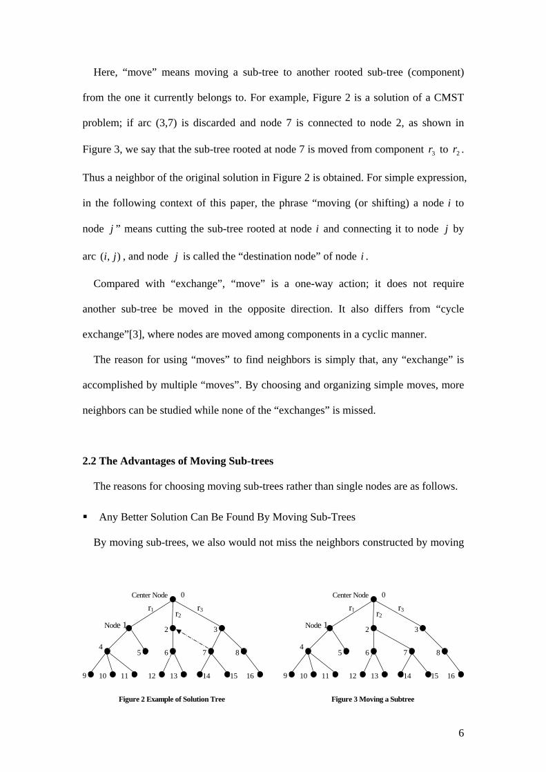
Here, “move” means moving a sub-tree to another rooted sub-tree (component)
from the one it currently belongs to. For example, Figure 2 is a solution of a CMST
problem; if arc (3,7) is discarded and node 7 is connected to node 2, as shown in
Figure 3, we say that the sub-tree rooted at node 7 is moved from component to .
Thus a neighbor of the original solution in Figure 2 is obtained. For simple expression,
in the following context of this paper, the phrase “moving (or shifting) a node i to
node
3r 2r
j ” means cutting the sub-tree rooted at node i and connecting it to node j by
arc , and node ),( ji j is called the “destination node” of node i .
Compared with “exchange”, “move” is a one-way action; it does not require
another sub-tree be moved in the opposite direction. It also differs from “cycle
exchange”[3], where nodes are moved among components in a cyclic manner.
The reason for using “moves” to find neighbors is simply that, any “exchange” is
accomplished by multiple “moves”. By choosing and organizing simple moves, more
neighbors can be studied while none of the “exchanges” is missed.
2.2 The Advantages of Moving Sub-trees
The reasons for choosing moving sub-trees rather than single nodes are as follows.
Any Better Solution Can Be Found By Moving Sub-Trees
By moving sub-trees, we also would not miss the neighbors constructed by moving
3
10
Center Node
Node 1
r1 r2 r3
2
45 6 7 8
0
Figure 2 Example of Solution Tree
9 11 12 13 14 15 16
15
3
10
Center Node
Node 1
r1 r2r3
2
45 6 7 8
0
Figure 3 Moving a Subtree
9 11 12 13 14 16
6
single nodes. This is because that, moving a single node form one component to
another can be done by moving the sub-tree rooted at this node to the other
component, and moving the descendent sub-trees of this node back to the original
component.
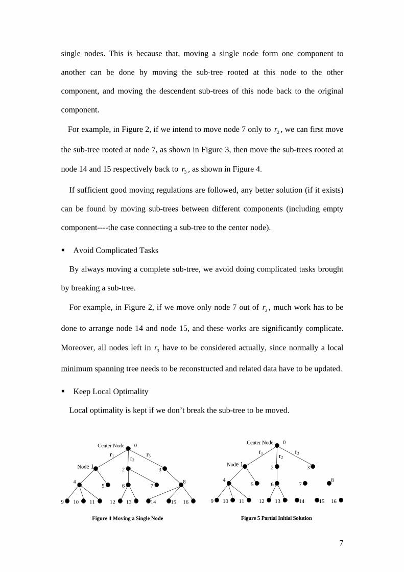
For example, in Figure 2, if we intend to move node 7 only to , we can first move
the sub-tree rooted at node 7, as shown in Figure 3, then move the sub-trees rooted at
node 14 and 15 respectively back to , as shown in Figure 4.
2r
3r
If sufficient good moving regulations are followed, any better solution (if it exists)
can be found by moving sub-trees between different components (including empty
component----the case connecting a sub-tree to the center node).
Avoid Complicated Tasks
By always moving a complete sub-tree, we avoid doing complicated tasks brought
by breaking a sub-tree.
For example, in Figure 2, if we move only node 7 out of , much work has to be
done to arrange node 14 and node 15, and these works are significantly complicate.
Moreover, all nodes left in have to be considered actually, since normally a local
minimum spanning tree needs to be reconstructed and related data have to be updated.
3r
3r
Keep Local Optimality
Local optimality is kept if we don’t break the sub-tree to be moved.
8
15
3
10
Center Node
Node 1
r1 r2r3
2
45 6 7
0
Figure 5 Partial Initial Solution
9 11 12 13 14 16
8
15
3
10
Center Node
Node 1
r1 r2 r3
2
45 6 7
0
Figure 4 Moving a Single Node
9 11 12 13 14 16
7

In Figure 2, suppose arc (7,14) is the cheapest arc among all arcs reaching node 14,
arc (7,15) is the cheapest arc reaching node 15, then disconnecting node 14 and node
15 from node 7 and connecting them to other nodes will definitely cause an increase
in the total cost of the solution.
This is more often the case when the solution is already very good. In other words,
as the solution is getting closer to the optimal solution, it is more likely that more
nodes have been linked in a more reasonable way. So, in the search process, when we
consider that we may get a cheaper cost solution by moving a node, we would rather
move the whole sub-tree rooted at this node, in order to avoid doing complicated
works that most probably will not lead to a better solution.
Fast Computation
The total cost of a solution has to be always monitored in the entire search process,
and with each sub-tree move, the change of the solution cost is exactly the difference
of the costs between two arcs. For example, in Figure 2, if node 7 is moved to node 2,
then the change of the total cost is just the difference between and . It is also
quick to change the topology of the tree by just changing an arc, no matter what kind
of data structure used. This has great significance for the related computations.
2,7c 3,7c
2.3 The Sub-Tree Move
There are many ways to perform the sub-tree move and certainly we prefer ways
that are more robust, or in another word, efficient. To find an efficient method, which
leads to better solutions in less iteration, the following aspects are considered.
Sequence of Nodes Being Added to the Initial Solution
8

Nodes are added to the initial solution in a sequence. Due to the way the initial
solution is constructed, we consider that nodes being added earlier have less chance to
be connected to a nearer ancestor.
Definition We say node j is nearer to node i if the cost of arc is cheaper than
arc where k is one of some other nodes. We define node
),( ji
),( ki j to be the nearest
node of node i if arc is the cheapest arc among all arcs reaching node . ),( ji i
Suppose the tree in Figure 2 is an initial solution of a certain problem, node 3 is the
first node being added to the initial solution.
According to the greedy initial solution generation algorithm, node 3 is the nearest
node of node 0, this means arc (0, 3) is the cheapest arc among all arcs reaching node
0. However, node 0 may not be the nearest node of node 3, that is, arc (0, 3) may not
be the cheapest arc reaching node 3.
Suppose node 1 is the second nearest node of node 0 and arc (0,1) is cheaper than
arc (1,3); then, the algorithm will connect node 1 to node 0.
Suppose the sequence of the nodes from the nearest to the furthest to node 3 is as
follows:
{4, 5, 9, 10, 11, 6, 12, 13, 7, 8, 14, 15, 16, 1, 2, 0} (6)
We make the following assumptions:
The third nearest node to node 0 is node 2.
The nearest node to nodes 2 is node 6.
The first two nearest nodes to node 1 are nodes 4 and 5.
The first two nearest nodes to node 1 are nodes 12 and 13.
The first three nearest nodes to node 4 are nodes 9, 10, and 11.
9

Arcs (0,2), (1,4), (1,5), (9,4), (10,4), (11,4), (2,6), (12,6) and (13,6) are cheaper
than arcs (2,3), (4,3), (5,3), (9,3), (10,3), (11,3), (6,3), (12,3) and (13,3)
respectively.
Then, following the initial solution generation algorithm, the next 9 nodes added
are nodes 2, 4, 5, 6, 9, 10, 11, 12 and 13, as shown in Figure 5.
We can see that none of the first 8 nodes in (6) can be connected to node 3, since
that will create a cycle.
On the other hand, a node being added to the initial solution later has more chance
to be connected to a nearer ancestor. Suppose in Figure 2, node 16 is the last node
added to the solution. Then, node 8 must be its nearest node (otherwise the modified
Dilkstra’s algorithm will not choose to connect node 16 to node 8, but node 16’s
nearest node i , since arc ( , 6) is cheaper than arc (8,16)). This is not true only if
node i is in a rooted sub-tree that is full (the central arc has reached its capacity).
i
Therefore, moving a node that was included in the solution earlier, will generally
lead to a greater decrease in the solution cost.
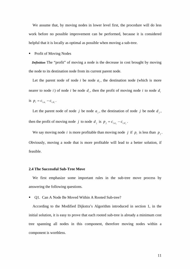
Level of Nodes
We define the level of a leaf node in a solution tree to be 0 (lowest level), and if a
node is in level l , then its parent node is in level 1+l . If a node has more than one
level value by counting from different leaves, we define the greater one to be its level.
Figure 6 shows the level (in brackets) of some nodes in Figure 2.
This definition is totally different from the traditional one, in which the “level” of
nodes in a tree is defined from top to bottom with the root being in level 0, and its
children being in level 1 etc. This is because it is concerned here how far a node is
from the leaves, but not from the root.
10
We assume that, by moving nodes in lower level first, the procedure will do less
work before no possible improvement can be performed, because it is considered
helpful that it is locally as optimal as possible when moving a sub-tree.
Profit of Moving Nodes
Definition The “profit” of moving a node is the decrease in cost brought by moving
the node to its destination node from its current parent node.
Let the parent node of node i be node , the destination node (which is more
nearer to node i ) of node i be node , then the profit of moving node i to node
is .
ia
id id
ii diaii ccp ,, −=
Let the parent node of node j be node , the destination of node ja j be node ,
then the profit of moving node
jd
j to node is jdjj diaij ccp ,, −= .
We say moving node is more profitable than moving node i j if is less than .
Obviously, moving a node that is more profitable will lead to a better solution, if
feasible.
ip jp
2.4 The Successful Sub-Tree Move
We first emphasize some important rules in the sub-tree move process by
answering the following questions.
Q1. Can A Node Be Moved Within A Rooted Sub-tree?
According to the Modified Dijkstra’s Algorithm introduced in section 1, in the
initial solution, it is easy to prove that each rooted sub-tree is already a minimum cost
tree spanning all nodes in this component, therefore moving nodes within a
component is worthless.
11
But when a sub-tree is moved into a component, this destination component may no
longer be a minimum spanning tree. In this case, this component is adjusted to a
minimum spanning tree. This MST adjustment is not performed in the sequence
priority search procedure, which will be introduced in Section 3, since otherwise the
nodes will lose their sequence property, according to which the searching is
performed.
Q2. What To Do If A Move Leads To An Infeasible Solution?
When a move causes the destination component containing too many nodes, one or
more sub-trees have to be moved out to make the component feasible. There are two
main concerns when deciding which node to be moved out. One is the profit of
moving the node; the other is the feasibility after moving the node. We consider that
making the solution feasible is more important. Thus the following rule is applied
when choosing the node to be moved out:
In the infeasible component, we move out the sub-tree containing the least number
of nodes and at the same time making the component feasible after being moved out.
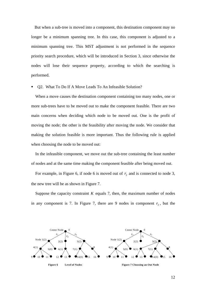
For example, in Figure 6, if node 6 is moved out of and is connected to node 3,
the new tree will be as shown in Figure 7.
2r
Suppose the capacity constraint K equals 7, then, the maximum number of nodes
in any component is 7. In Figure 7, there are 9 nodes in component , but the 3r
14(0)
2(2)
8
15
3(2)
10
Center Node
Node 1(2)
r1 r2 r3
4(1) 5(0) 6(1) 7(1)
0
Figure 6 Level of Nodes
9 11 12 13 16
14(0)
2(2)
8
15
3(2)
10
Center Node
Node 1(2)
r1 r2r3
4(1)5(0) 6(1) 7(1)
0
Figure 7 Choosing an Out Node
9 11 12 13 16
12

capacity constraint is 7, so at least 2 nodes have to be moved out of to make this
component feasible.
3r
In , We can move out node 7, node 8 or node 3, because the number of nodes in
the sub-trees rooted at these nodes are 3, 2 and 9 respectively and are all greater than
or equal to 2. Since the sub-tree rooted at node 8 contains the least number of nodes (2
nodes), we choose to move out node 8 to look for a lower possibility of getting an
infeasible solution after moving node 8 into other components.
3r
Q3. Can A Node Be Moved Back To Its Original Component?
In order to make sure that no endless moving cycles occur, a node cannot be moved
back into its original component.
For clear interpretation, the following expressions will be used in the later context.
“Shift”: given a certain node i and its destination node j , “shift” node i to j
refers to the single moving action, in which the sub-tree rooted at node i is cut and
connected to node j in another component by arc . ),( ji
“Move”: given a certain node i and its destination node j , one “move” refers to
not only the action of shifting node i to node j , but also the consequent node shifting
for looking for a feasible solution, if shifting node i to node j makes the solution
infeasible.
“Successful move”: if one move finds a feasible better solution before the
termination criterion is satisfied, we say this move is a successful move.
“Importer (exporter)”: if a node has been moved in (out of) a component, we say
this component has been changed, and has acted as an importer (exporter).
Regarding Q3, the actual rule in the searching process is that, a node can be moved
into a changed component, which has act as an exporter, only if this single import
13
action makes the solution feasible and therefore ends a successful move. After all
components have been changed, a move is forced to terminate whether it is successful
or not.
2.5 The Move Procedure
Suppose we are going to move node i to node j , we call node i the “Origin Node”,
and node j the “Destination Node”. We also call a node “Out Node” if the sub-tree
rooted at this node is chosen to move out of its current component.
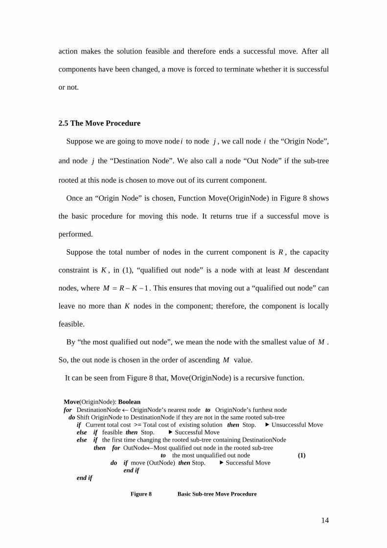
Once an “Origin Node” is chosen, Function Move(OriginNode) in Figure 8 shows
the basic procedure for moving this node. It returns true if a successful move is
performed.
Suppose the total number of nodes in the current component is R , the capacity
constraint is K , in (1), “qualified out node” is a node with at least M descendant
nodes, where 1−−= KRM . This ensures that moving out a “qualified out node” can
leave no more than K nodes in the component; therefore, the component is locally
feasible.
By “the most qualified out node”, we mean the node with the smallest value of M .
So, the out node is chosen in the order of ascending M value.
It can be seen from Figure 8 that, Move(OriginNode) is a recursive function.
Move(OriginNode): Boolean for DestinationNode ← OriginNode’s nearest node to OriginNode’s furthest node do Shift OriginNode to DestinationNode if they are not in the same rooted sub-tree if Current total cost >= Total cost of existing solution then Stop. Unsuccessful Move else if feasible then Stop. Successful Move else if the first time changing the rooted sub-tree containing DestinationNode then for OutNode←Most qualified out node in the rooted sub-tree
to the most unqualified out node (1) do if move (OutNode) then Stop. Successful Move end if end if
Figure 8 Basic Sub-tree Move Procedure
14

3 The Algorithm
As introduced in section 2.3, we consider nodes are different in three aspects, the
sequence of being added to the solution, the level value and the potential profit of
moving the nodes. Based on the basic move function presented in section 2.5, four
algorithms for the CMST problem are developed.
Sequence Priority Search
Let N be the problem size, that is, the total number of nodes (excluding center
node).
After constructing the initial solution, all nodes are stored in an array
NodeSequence[1..N] in the order of the sequence being linked to the solution tree.
NodeSequence[1] is the first node linked to the center, and NodeSequence[N] is the
last node spanned.
The sequence priority search procedure is as follows:
for OriginNode ← NodeSequence[1] to NodeSequence[N]
do Move(OriginNode)
Level Priority Search
Let “UnSuccess” stores the number of successive times of unsuccessful move, L be
the current active level, the level priority search procedure is shown in Figure 9.
Line (1) shows the termination condition. For N-node problem, if N times of
successive unsuccessful move have been performed, then we know no improved
solution can be found by moving any of the nodes.
15
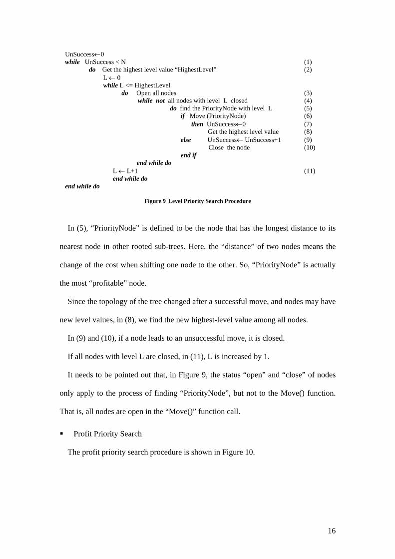
UnSuccess←0 while UnSuccess < N (1)
do Get the highest level value “HighestLevel” (2) L ← 0 while L <= HighestLevel do Open all nodes (3) while not all nodes with level L closed (4) do find the PriorityNode with level L (5) if Move (PriorityNode) (6)
then UnSuccess←0 (7) Get the highest level value (8)
else UnSuccess← UnSuccess+1 (9) Close the node (10)
end if end while do
L ← L+1 (11) end while do end while do
Figure 9 Level Priority Search Procedure
In (5), “PriorityNode” is defined to be the node that has the longest distance to its
nearest node in other rooted sub-trees. Here, the “distance” of two nodes means the
change of the cost when shifting one node to the other. So, “PriorityNode” is actually
the most “profitable” node.
Since the topology of the tree changed after a successful move, and nodes may have
new level values, in (8), we find the new highest-level value among all nodes.
In (9) and (10), if a node leads to an unsuccessful move, it is closed.
If all nodes with level L are closed, in (11), L is increased by 1.
It needs to be pointed out that, in Figure 9, the status “open” and “close” of nodes
only apply to the process of finding “PriorityNode”, but not to the Move() function.
That is, all nodes are open in the “Move()” function call.
Profit Priority Search
The profit priority search procedure is shown in Figure 10.
16

while Runtime < GivenTime (1) do Open all pairs of nodes while Not all pairs of nodes closed do Find the PriorityNode Find the DestinationNode of the PriorityNode Move1(PriorityNode, DestinationNode ) (2) if Successful
then Close the node pair (PriorityNode, DestinationNode)
Figure 10 Profit Priority Search Procedure
Same as in the level priority search procedure, “PriorityNode” is the node which
has the longest distance to its nearest node in other rooted sub-trees; “open” and
“close” only apply to finding a “PriorityNode”.
“DestinationNode” is PriorityNode’s nearest node in other rooted sub-trees.
In (1), a given running time is used as the termination criterion, since all nodes are
opened again once they have been all closed.
In (2), function Move1 performs one shift from the “PriorityNode” to the
“DestinationNode”, and then calls the basic Move(OriginNode) function, in which all
possible destination nodes are considered.
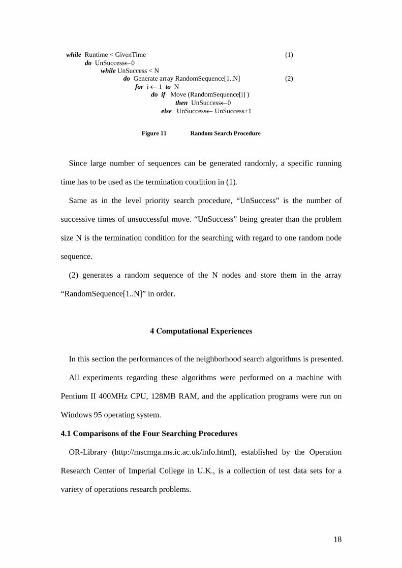
Random Search Procedure
Besides the above three procedures, we would also like to implement a random
search procedure.
All properties of the nodes are disregarded and the nodes are just arranged in a
random sequence. Then the basic Move(OriginNode) function is called with respect to
this node sequence.
We assumes that the random search procedure may find better solutions in some
instances. But generally, the first three procedures will perform better, since the
author considers that they are more robust due to the analyses in the previous sections.
Figure 11 shows how the random search procedure is performed.
17
while Runtime < GivenTime (1) do UnSuccess←0 while UnSuccess < N do Generate array RandomSequence[1..N] (2) for i ← 1 to N do if Move (RandomSequence[i] )
then UnSuccess←0 else UnSuccess← UnSuccess+1
Figure 11 Random Search Procedure
Since large number of sequences can be generated randomly, a specific running
time has to be used as the termination condition in (1).
Same as in the level priority search procedure, “UnSuccess” is the number of
successive times of unsuccessful move. “UnSuccess” being greater than the problem
size N is the termination condition for the searching with regard to one random node
sequence.
(2) generates a random sequence of the N nodes and store them in the array
“RandomSequence[1..N]” in order.
4 Computational Experiences
In this section the performances of the neighborhood search algorithms is presented.
All experiments regarding these algorithms were performed on a machine with
Pentium II 400MHz CPU, 128MB RAM, and the application programs were run on
Windows 95 operating system.
4.1 Comparisons of the Four Searching Procedures
OR-Library (http://mscmga.ms.ic.ac.uk/info.html), established by the Operation
Research Center of Imperial College in U.K., is a collection of test data sets for a
variety of operations research problems.
18
The popular benchmark CMST problems in OR-Library are used to test the
algorithms.
Table 1 is the results of implementing Sequence Priority Search, Level Priority
Search and Profit Priority Search procedures for solving one set of 41-node problems.
The capacity constraint is 10.
In Table 1, as well as in all other tables, the “optimal solution” refers to the optimal
solution found by the authors’ exact algorithms.
“N.S.M.” is the total number of successful moves.
It can be seen from Table 1 that, the running time before termination of the
Sequence Priority Search procedure is less than that of the Level Priority Search
procedure. However, the Sequence Priority Search procedure missed the optimal
solution for two problems, while the Level Priority Search procedure only missed one.
The Profit Priority Search procedure was run for 1 second, and it found the optimal
solutions for four problems from the five.
To test its performance, the Random Search procedure was run ten times for each
of the problems in Table 1, and the results are shown in Table 2.
From Table 2, we can see that the Random Search procedure found the optimal
solution for each problem within 10 runs. It even found the optimal solution for the
fifth problem, while none of the three procedures in Table 1 achieved so.
4.2 The Integrated Search Procedure
It can be seen from the above experiments that, as we have expected when
designing these algorithms, each algorithm has both advantages and disadvantages
compared with others. Therefore, we would integrate these search procedures into one
program, as shown in Figure 12.
19
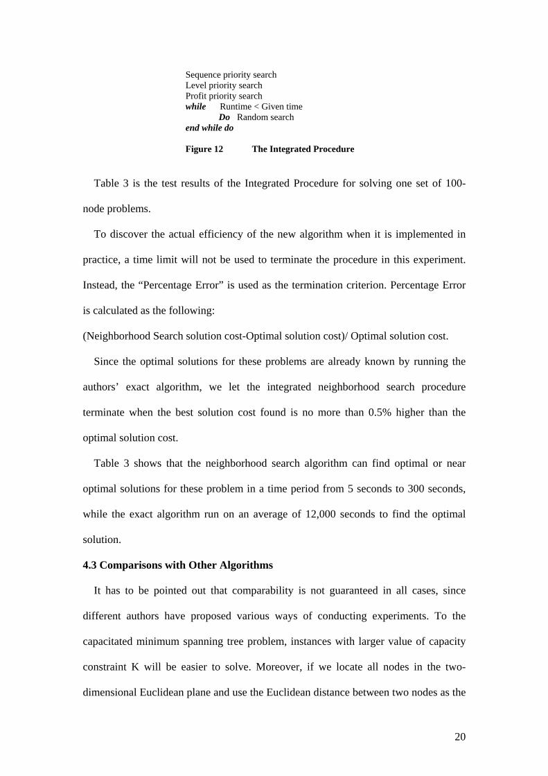
Sequence priority search Level priority search Profit priority search while Runtime < Given time
Do Random search end while do Figure 12 The Integrated Procedure
Table 3 is the test results of the Integrated Procedure for solving one set of 100-
node problems.
To discover the actual efficiency of the new algorithm when it is implemented in
practice, a time limit will not be used to terminate the procedure in this experiment.
Instead, the “Percentage Error” is used as the termination criterion. Percentage Error
is calculated as the following:
(Neighborhood Search solution cost-Optimal solution cost)/ Optimal solution cost.
Since the optimal solutions for these problems are already known by running the
authors’ exact algorithm, we let the integrated neighborhood search procedure
terminate when the best solution cost found is no more than 0.5% higher than the
optimal solution cost.
Table 3 shows that the neighborhood search algorithm can find optimal or near
optimal solutions for these problem in a time period from 5 seconds to 300 seconds,
while the exact algorithm run on an average of 12,000 seconds to find the optimal
solution.
4.3 Comparisons with Other Algorithms
It has to be pointed out that comparability is not guaranteed in all cases, since
different authors have proposed various ways of conducting experiments. To the
capacitated minimum spanning tree problem, instances with larger value of capacity
constraint K will be easier to solve. Moreover, if we locate all nodes in the two-
dimensional Euclidean plane and use the Euclidean distance between two nodes as the
20
cost of the arc between them, we say the root is “in the center” or “in the corner”
when its location is in the center of the Euclidean plane or in the corner of the
Euclidean plane. Another parameter, which has considerable impact on the
performance of most algorithms, is the location of the root. For problem instances in
OR-Library, class “tc” refers to problems with the root in the center of the Euclidean
plane and class “te” refers to problems with the root in the corner of the Euclidean
plane. It is believed that “tc” class problems are relatively “easier” to be solved than
“te” class problems.
The best published heuristics for the capacitated minimum spanning tree problem is
Ahuja et al’s Multi-exchange Neighborhood Search algorithm [1]. As the most recent
lower bound algorithms, Gouveia and Martins’ hop-indexed models [11] [12] have
the best overall performances. Referring to the benchmark problems in OR-Library,
Ahuja et al’s algorithm and Gouveia and Martins’ algorithm found the same solutions
for all “tc” class problems in similar computational time; but Ahuja et al’s algorithm
found better solutions for 3 “te” class problems in much less computational time.
Table 4 and 5 are comparisons of the Integrated Neighborhood Search algorithm
and the Multi-exchange Neighborhood Search algorithm.
The problems in table 4 are the 41-node “tc” class benchmark problems in OR-
Library, and the problems in Table 5 are the 41-node “te” class problems. The
capacity constraint is 10.
The program for the Multi-exchange Neighborhood Search algorithm was run on a
DEC Alpha computer.
It can be seen from Table 4 that, the Integrated Neighborhood Search algorithm is
faster when solving the “tc” class problems. For the “te” class problems however, it
21
has to run 1000 seconds to get the same solutions found by the Multi-exchange
Neighborhood Search algorithm. This is shown in Table 5.
The latest achievement is Ahuja et al’s Composite Very Large-scale Neighborhood
Structure for the CMST problem [2].
Table 6 is a comparison of the Integrated Neighborhood Search algorithm and the
Composite Very Large-scale Neighborhood Search algorithm for solving the 81-node
“tc” class benchmark problems in OR-Library.
Table 7 is the comparison of the two algorithms for solving the 81-node “te” class
problems. The capacity constraints are both 20 in these two tests.
The Composite Very Large-scale Neighborhood Search algorithm was tested on a
Pentium 4 processor with 512 MB RAM and 256KB L2 cache, while the author’s
programs were run on a machine with Pentium II CPU and 128 MB RAM.
From Table 6, we can see that the Integrated Neighborhood Search algorithm is
sufficiently faster to find the currently known best solutions.
However, Table 7 shows that for the “te” class problems, the Integrated
Neighborhood Search algorithm could not find solutions as good as those found by
the Composite Very Large-scale Neighborhood Search algorithm in the same time
period.
4.4 Analyses of the Neighborhood Search Algorithms
For the CMST problems maintained in OR-Library, it is considered that, the “tc”
class problems are relatively “easier” to be solved than the “te” class problems.
From the test results shown in section 4.3, it is noticed that the authors’
neighborhood search algorithm, compared with other algorithms, performs better for
“easier” problems, but worse for relatively “harder” problems. We consider that the
reasons are as follows.
22
According to the search routines introduced in the previous sections, the authors’
algorithm is concerned very much with the characteristics of current and consequent
solutions and makes effort on fast improving of the initial solution.
In the Multi-exchange Neighborhood Search algorithm and the Composite Very
Large-scale Neighborhood Search algorithm, much work is done to construct the
“improvement graph” and find the “valid cycles”, which are node exchanges leading
to better solutions.
Therefore, the authors’ neighborhood search algorithm is faster, but may not find
solutions as good as those found by the other two algorithms, since it does not
perform those precise “valid cycle” detections.
The authors’ neighborhood search algorithm has the same complexity with the
Composite Very Large-scale Neighborhood Search algorithm, which is ,
where is the problem size and
))/(( rrnΟ
n r is the total number of rooted sub-trees.
Since in the Integrated Neighborhood Search algorithm, the basic procedure is a
recursive function, the authors’ computer will run out of memory if the capacity
constraint is very small and therefore the r value is very large.
5 Summary
We have proposed a neighborhood search algorithm for the capacitated minimum
spanning tree problem and have presented the comparisons between different
algorithms. We introduced a series of new sub-tree move procedures, interpreted their
principles and analyzed their advantages. Computation experiences show that the
proposed procedures perform better than existing algorithms for relatively easier
problem. There is room for further improvement in our future work, especially in
dealing with relatively harder CMST problems.
23
References
[1] Ahuja, R.K., Orlin, J.B. and Sharma, D. (2001). Multi exchange neighborhood
search algorithms for the capacitated minimum spanning tree problem. Mathematical
Programming 91: 9-39.
[2] Ahuja, R.K., Orlin, J.B. and Sharma, D. (2001). A composite neighborhood search
algorithm for the capacitated minimum spanning tree problem. Working paper.
[3] Ahuja, R.K., Orlin, J.B. and Sharma, D. (2000). “Very large-scale neighborhood
search”. Operational Research 7: 301-317.
[4] Altinkemer, K. and Gavish, B. (1988). Heuristics with constant error guarantees
for the design of tree networks. Management Science 32: 331 - 341.
[5] Amberg, A., Domscheke, W. and Braunschweig, S. (1996). Capacitated Minimum
Spanning Trees: Algorithms using intelligent search. Combinatorial optimization:
Theory and Practice 1: 9-39.
[6] Elias, D. and Ferguson, M.J. (1974). Topological design of multipoint
teleprocessing networks. IEEE Transactions on Communications 22: 1753 - 1762.
[7] Frank, H., Frisch, I.T., Van Slyke, R. and Chou, W.S. (1971). Optimal design of
centralized computer design network. Networks 1: 43-57.
[8] Gavish, B. (1991). Topological design of telecommunication networks-local
access design methods. Annals of Operations Research 33: 17-71.
[9] Gavish, B. and Altinkemer, K. (1986). Parallel savings heuristics for the
topological design of local access tree networks. Proc. IEEE INFOCOM 86
Conference: 130-139.
24
[10] Gouveia, L. and Paixao, J. (1991). Dynamic programming based heuristics for
the topological design of local access networks. Annals of Operations Research 33:
305-327.
[11] Gouveia, L. and Martins, P. (1999). The capacitated minimum spanning tree
problem: An experiment with a hop-indexed model. Ann Oper Res 86: 271-294.
[12] Gouveia, L. and Martins, P. (2000). A hierarchy of hop-indexed models for the
capacitated minimum spanning tree problem. Networks 35: 1-16.
[13] Karnaugh, M. (1976). A new class of algorithms for multipoint network
optimization. IEEE Transactions on Communications 24: 500-505.
[14] Papadimitriou, C.H. (1978). The Complexity of the capacitated tree problem.
Networks 8: 217-230.
[15] Schneider, G.M. and Zastrow, M.N. (1982). An algorithm for the design of
multilevel concentrator networks. Computer Networks 6: 1-11.
[16] Sharma, R.L. and El-Bardai, M.T. (1970). Suboptimal communications network
synthesis. Proc. 1970 Int. Conf. Comm. 19: 11-16.
[17] Thangiah, S.R., Osman, I.H. and Sun, T. (1994). Hybrid genetic algorithms,
simulated annealing and tabu search methods for vehicle routing problems with time
windows. Working Paper, Univ. of Kent, Canterbury.
25
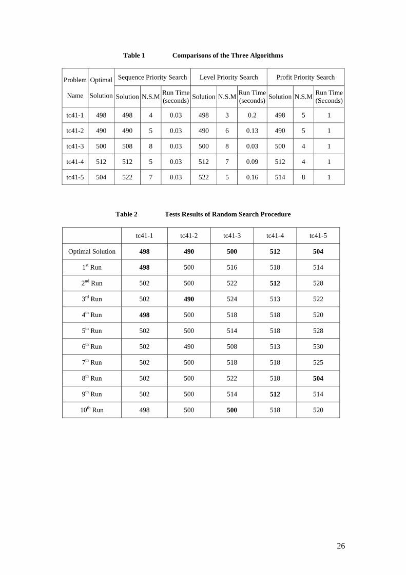
Table 1 Comparisons of the Three Algorithms
Sequence Priority Search Level Priority Search Profit Priority Search Problem
Name
Optimal
Solution Solution N.S.M Run Time(seconds) Solution N.S.M Run Time
(seconds) Solution N.S.M Run Time(Seconds)
tc41-1 498 498 4 0.03 498 3 0.2 498 5 1
tc41-2 490 490 5 0.03 490 6 0.13 490 5 1
tc41-3 500 508 8 0.03 500 8 0.03 500 4 1
tc41-4 512 512 5 0.03 512 7 0.09 512 4 1
tc41-5 504 522 7 0.03 522 5 0.16 514 8 1
Table 2 Tests Results of Random Search Procedure
tc41-1 tc41-2 tc41-3 tc41-4 tc41-5
Optimal Solution 498 490 500 512 504
1st Run 498 500 516 518 514
2nd Run 502 500 522 512 528
3rd Run 502 490 524 513 522
4th Run 498 500 518 518 520
5th Run 502 500 514 518 528
6th Run 502 490 508 513 530
7th Run 502 500 518 518 525
8th Run 502 500 522 518 504
9th Run 502 500 514 512 514
10th Run 498 500 500 518 520
26
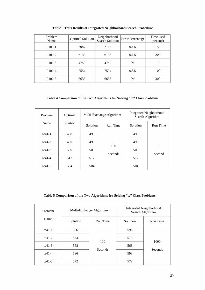
Multi-Exchange Algorithm Integrated Neighborhood Search Algorithm Problem
Name
Optimal
Solution Solution Run Time Solution Run Time
tc41-1 498 498 498
tc41-2 490 490 490
tc41-3 500 500 500
tc41-4 512 512 512
tc41-5 504 504
100
Seconds
504
1
Second
Multi-Exchange Algorithm Integrated Neighborhood Search Algorithm Problem
Name
Solution Run Time Solution Run Time
te41-1 596 596
te41-2 573 573
te41-3 568 568
te41-4 596 598
te41-5 572
100
Seconds
572
1000
Seconds
Table 5 Comparison of the Two Algorithms for Solving “te” Class Problems
Table 4 Comparison of the Two Algorithms for Solving “tc” Class Problems
Table 3 Tests Results of Integrated Neighborhood Search Procedure
Problem Name Optimal Solution Neighborhood
Search Solution Error Percentage Time used (second)
P100-1 7087 7117 0.4% 5
P100-2 6133 6138 0.1% 200
P100-3 4759 4759 0% 10
P100-4 7554 7594 0.5% 100
P100-5 6635 6635 0% 300
27
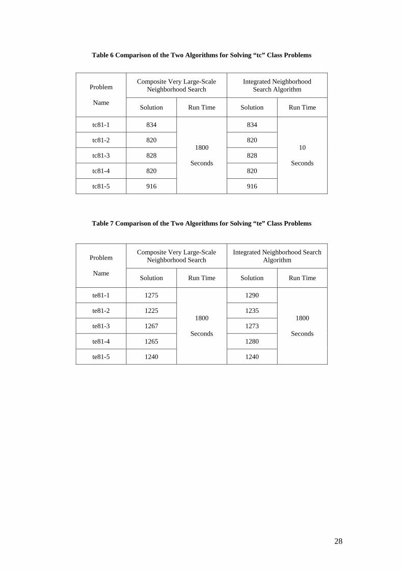
Table 6 Comparison of the Two Algorithms for Solving “tc” Class Problems
Composite Very Large-Scale Neighborhood Search
Integrated Neighborhood
Search Algorithm Problem
Name Solution Run Time Solution Run Time
tc81-1 834 834
tc81-2 820 820
tc81-3 828 828
tc81-4 820 820
tc81-5 916
1800
Seconds
916
10
Seconds
Table 7 Comparison of the Two Algorithms for Solving “te” Class Problems
Composite Very Large-Scale Neighborhood Search
Integrated Neighborhood Search Algorithm Problem
Name
Solution Run Time Solution Run Time
te81-1 1275 1290
te81-2 1225 1235
te81-3 1267 1273
te81-4 1265 1280
te81-5 1240
1800
Seconds
1800
Seconds
1240
28