Embed Size (px)
Citation preview
New Benchmark Instancesfor the Capacitated Vehicle Routing Problem
Eduardo Uchoa*1, Diego Pecin2, Artur Pessoa1, Marcus Poggi2,
Anand Subramanian3, Thibaut Vidal2
1 Universidade Federal Fluminense, Departamento de Engenharia de Producao, Brazil2 Pontifıcia Universidade Catolica do Rio de Janeiro, Departamento de Informatica, Brazil
3 Universidade Federal da Paraıba, Departamento de Engenharia de Producao, Brazil
Abstract. The recent research on the CVRP is being slowed down by the lack of a goodset of benchmark instances. The existing sets suffer from at least one of the followingdrawbacks: (i) became too easy for current algorithms; (ii) are too artificial; (iii) are toohomogeneous, not covering the wide range of characteristics found in real applications.We propose a new set of instances ranging from 100 to 1000 customers, designed in orderto provide a more comprehensive and balanced experimental setting. We report resultswith state-of-the-art exact and heuristic methods.
Keywords. Vehicle Routing Problem, Benchmark Instances, Experimental Analysis ofAlgorithms
* Corresponding author
1
1 Introduction
The Vehicle Routing Problem (VRP) is among the most widely studied problems in the
fields of operations research and combinatorial optimization. Its relevance stems from its
direct application in the real world systems that distribute goods and provide services,
vital to the modern economies. Reflecting the large variety of conditions present in those
systems, the VRP literature is spread into dozens of variants. For example, there are
variants that consider time windows, multiple depots, mixed vehicle fleet, split delivery,
pickups and deliveries, precedences, complex loading constraints, etc.
In the vast landscape of VRP variants, the Capacitated VRP (CVRP) occupies a
central position. It was defined by Dantzig and Ramser [12] as follows. The input consists
of a set of n + 1 points, a depot and n customers; an (n + 1)× (n + 1) matrix d = [dij]
with the distances between every pair of points i and j; an n-dimensional demand vector
q = [qi] giving the amount to be delivered to customer i; and a vehicle capacity Q. A
solution is a set of routes, starting and ending at the depot, that visit every customer
exactly once in such a way that the sum of the demands of the customers of each route
does not exceed the vehicle capacity. The objective is to find a solution with minimum
total route distance. Some authors also assume that the number of routes is fixed to an
additional input number K (almost always defined as the minimum possible number of
routes, Kmin).
The CVRP plays a particular role on VRP algorithmic research, for both exact and
on heuristics methods. Being the most basic variant, it is a natural testbed for trying
new ideas. Its relative simplicity allows cleaner descriptions and implementations, without
the additional conceptual burden necessary to handle more complex variants. Successful
ideas for the CVRP are often later extended to more complex variants. For example, the
classical CVRP heuristic by Clarke and Wright [9] was adapted for the VRP with Time
Windows [29] and for many other variants, as surveyed in Rand [25].
The present work is motivated by the claim that the recent research on the CVRP is
being hampered by the lack of a well-established set of benchmark instances able to push
the limits of the state-of-the-art algorithms. Let us examine this claim:
• Since Augerat et al. [3], nearly all new exact methods for the CVRP have been
tested over instances from six different classes. Classes A, B and P were proposed in [3],
while classes E, F and M were proposed by Christofides and Eilon [7], by Fisher [13] and
by Christofides et al. [8], respectively. Nearly all those instances are Euclidean. In the

literature of exact methods it became usual to follow the TSPLIB convention of rounding
distances to the nearest integer [26] and also to fix the number of routes.
The ABEFMP instances provided a good benchmark until the mid 2000’s decade.
Although 90 out of its 95 instances have no more than 100 customers, several such instances
were still very challenging for the branch-and-cut algorithms (like [1, 2, 3, 6, 20, 24, 34])
which prevailed at that time. Then, the branch-cut-and-price of Fukasawa et al. [14] solved
all its instances with up to 100 customers, as well as instances M-n121-k7 and F-n135-k7
(the later was already solved since [3]). Only instances M-n151-k12, M-n200-k16 and
M-n200-k17 remained unsolved. From that moment, the benchmark was not satisfactory
anymore. While the majority of its instances became quite easy, the now more interesting
range of 101 to 200 customers was very thinly populated. In particular, the column and cut
generation algorithms of Baldacci et al. [4, 5] significantly reduced the CPU time required
to solve many ABEFMP instances, but could not solve the three larger M instances. Later,
the algorithms of Contardo and Martinelli [10] and Røpke [28] were capable of solving
M-n151-k12. Very recently, the algorithm of Pecin et al. [22] solved the last two open
instances in the benchmark.
• Since the 1980’s, almost all articles proposing new heuristic and metaheuristic
methods for the CVRP reported results on a subset of the instances by Christofides and
Eilon [7] and Christofides et al. [8]. In this literature, it is usual to follow the convention
of not rounding the Euclidean distances and not to fix the number of routes. This classical
benchmark is also exhausted, since most recent heuristics find systematically the best
known solutions on nearly all instances. In fact, Rochat and Taillard [27] already published
in 1995 what we now know to be the optimal solutions, except on a single instance with
199 customers, where the reported solution was only 0.012% off-optimal.
The more recent set of instances by Golden et al. [17] is now the second most frequently
used benchmark. Having larger instances, ranging from 240 to 483 customers, it still has a
good discriminating power. In fact, the heuristics of Nagata and Braysy [21] and Vidal
et al. [32] are considered the best available for the CVRP basically due to their superior
performance on Golden’s instances. Nevertheless, we believe that those instances are not
sufficient for a good benchmark. A first drawback is their artificiality. In all instances
the customers are positioned in concentric geometric figures, either circles, squares or
six-pointed stars. The demands also follow very symmetric patterns. As a result, the
solution space is partitioned into groups of equivalent solutions obtainable by rotations
2

and flippings around several axis of symmetry. The second drawback is their relative
homogeneity. For example, there are no instances with clusters of customers.
This work proposes a new set of 100 instances, ranging from 100 to 1000 customers,
intended to be used by both exact and heuristic methods in the next years. They were
designed in order to provide a more comprehensive and balanced experimental setting.
The remainder of the paper is organized as follows. Section 2 summarizes the current
CVRP benchmark instances. Section 3 explains the procedure developed for generating
new CVRP instances. Section 4 contains the results found by state-of-the-art heuristic
and exact methods for the new set of instances. Section 5 briefly describes the features
of the new CVRPLIB web site where all instances mentioned in this paper are available.
Finally, Section 6 presents the concluding remarks of this work.
2 Current Benchmark Instances
In this section we provide detailed information about the existing benchmark instances.
In particular, we tried to track back the generation process of all these instances.
Table 1 presents data regarding the E series. Although they are usually attributed to
Christofides and Eilon [7], some instances actually come from Dantzig and Ramser [12]
and from Gaskell [15], and some are modifications later suggested by Gillett and Miller
[16]. As usual in the literature on exact methods, the naming of the instances reflects
the number of points (including the depot) and the fixed number of routes. For example,
E-n101-k8 is an instance with 100 customers and a requirement of 8 routes. Columns in
Table 1 include the value of Q, the tightness (the ratio between the sum of all demands and
KQ, the total capacity available in the fixed number of routes) and the optimal solution
value.
Table 2 presents information about the M series and explains how each instance was
generated. Instances M-n200-k16 and M-n200-k17 only differ by the required number
of routes. In fact, M-n200-k17 is the only ABEFMP instance where the fixed number
of routes does not match the minimum possible. This additional instance was created
because M-n200-k16 has a tightness so close to 1 (0.995625) that finding good feasible
solutions for it was very difficult. Surprisingly, it was recently discovered that the optimal
solution of M-n200-k16 costs less than the optimal solution of M-n200-k17 [22].
Table 3 presents the three real-world instances that compose the F series. Tables 4
and 5 correspond to the A and B series, respectively. While in the A series the customers
and the depot are randomly positioned; they are clustered in the B series. The instances
3
from series P were generated by taking some instances from the A, B and E series and
changing their capacities. Consequently, the required number of routes also changes. For
example, P-n101-k4 was obtained from E-n101-k8 by doubling the capacity.
Christofides et al. [8] defined the benchmark set shown in Table 7. Instances CMT1,
CMT2, CMT3, CMT, CMT5, CMT11 , and CMT12 correspond to instances E-n51-k5,
E-n76-k10, E-n101-k8, M-n151-k12, M-n200-k16, M-n121-k7, and M-n100-k10, respectively.
The only difference are the conventions: the euclidean distances are represented with full
computer precision (without rounding), and the number of routes is not fixed. This set
also contains instances for the duration constrained CVRP, obtained from the previous
CVRP instances by adding maximum route duration (MD) and service time (ST) values.
These values are also reported in Table 7. Column KBKS gives the number of routes in
the optimal/best known solution of each instance. Optimal solutions are marked with a *.
Table 8 corresponds to the benchmark proposed in Golden et al. [17]. There are 12
CVRP instances and 8 instances for Duration-constrained CVRP, the maximum durations
(as there are no service times, this is equivalent to a bound on the maximum total distance
traveled in a route) are given in column (MD). Table 8 also gives the geometric patterns
used for positioning the customers in each instance.
Table 9 corresponds to a benchmark proposed in Rochat and Taillard [27]. Twelve
instances from 75 to 150 customers were generated using a scheme where the depot is always
in the center, the customers are clustered and demands are taken from an exponential
distribution. An additional instance with 385 customers, obtained from real-world data,
already appeared in [31]. Note that a best value of 2341.84 for instance tai150c was
mentioned on some benchmark instance repositories and then relayed in some papers. Yet,
the exact algorithm of [22] determined that a solution of 2358.66 is optimal and most
recent heuristics found the same value. We thus assume that this previous solution was
erroneous.
Although there are no pure CVRP instances in this set, for the sake of completeness,
Table 10 presents a benchmark proposed in Li et al. [19], composed by 12 larger scale
instances of the Duration-constrained CVRP. Typical CVRP heuristics can be easily
adapted to handle duration/distance constraints, and some articles on the CVRP also
reported results in the Li benchmark. However, most recent state-of-the-art methods for
the CVRP [21, 32] did not. Therefore, in order to present solutions that correspond to
the current point of algorithmic evolution, we performed runs with the algorithm of [32].
Table 10 has been updated to include the newly found best known solutions. The detailed
computational results are reported in the Appendix. We also highlight an issue related
4
to the published solution of instance pr32, generated by a manual process in [19] with a
distance value of 36919.24. This solution seems to have 10 routes from the figure in the
paper, and as such cannot comply with the distance limit of 3600 units. For this reason, it
was not included in the table.
3 Newly Proposed Instances
This section describes how the instances in the proposed CVRP benchmark were generated.
As happens in almost all the existing instances, the distances are two-dimensional Euclidean.
Depot and costumers have integer coordinates corresponding to points in a [0, 1000] ×[0, 1000] grid. Each instance is characterized by the following attributes: number of
customers, depot positioning, customer positioning, demand distribution, and average
route size. The possible values of each attribute and their effect in the generation are
described in the next subsection.
3.1 Instance Attributes
3.1.1 Depot Positioning
Three different positions for the depot are considered:
Central (C) – depot in the center of the grid, point (500,500).
Eccentric (E) – depot in the corner of the grid, point (0,0).
Random (R) – depot in a random point of the grid.
The TC, TE and TR instances [18], used as benchmark on rooted network design problems,
present similar alternatives for root positioning.
3.1.2 Customer Positioning
Three alternatives for customer positioning are considered, following the R, C and RC
instance classes of the Solomon set for the VRPTW [29].
Random (R) – All customers are positioned in random points of the grid.
Clustered (C) – At first, a number S of customers that will act as cluster seeds is
picked from an uniform discrete distribution UD[3,8]. Next, the S seeds are randomly
positioned in the grid. The seeds will then attract, with an exponential decay, the
5
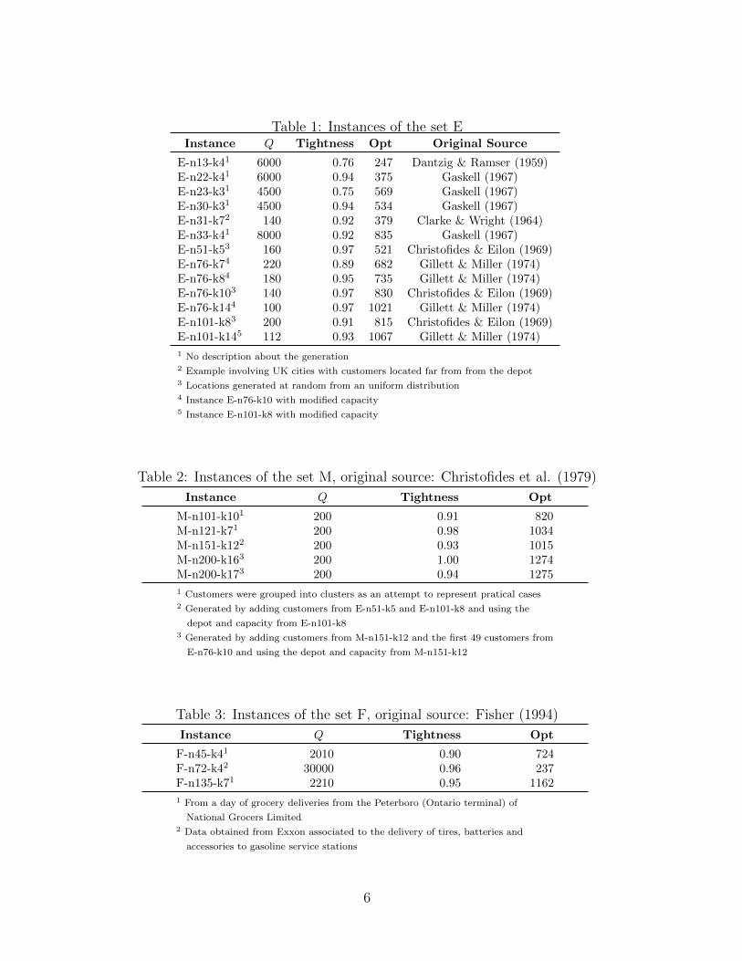
Table 1: Instances of the set EInstance Q Tightness Opt Original Source
E-n13-k41 6000 0.76 247 Dantzig & Ramser (1959)E-n22-k41 6000 0.94 375 Gaskell (1967)E-n23-k31 4500 0.75 569 Gaskell (1967)E-n30-k31 4500 0.94 534 Gaskell (1967)E-n31-k72 140 0.92 379 Clarke & Wright (1964)E-n33-k41 8000 0.92 835 Gaskell (1967)E-n51-k53 160 0.97 521 Christofides & Eilon (1969)E-n76-k74 220 0.89 682 Gillett & Miller (1974)E-n76-k84 180 0.95 735 Gillett & Miller (1974)E-n76-k103 140 0.97 830 Christofides & Eilon (1969)E-n76-k144 100 0.97 1021 Gillett & Miller (1974)E-n101-k83 200 0.91 815 Christofides & Eilon (1969)E-n101-k145 112 0.93 1067 Gillett & Miller (1974)
1 No description about the generation2 Example involving UK cities with customers located far from from the depot3 Locations generated at random from an uniform distribution4 Instance E-n76-k10 with modified capacity5 Instance E-n101-k8 with modified capacity
Table 2: Instances of the set M, original source: Christofides et al. (1979)
Instance Q Tightness Opt
M-n101-k101 200 0.91 820M-n121-k71 200 0.98 1034M-n151-k122 200 0.93 1015M-n200-k163 200 1.00 1274M-n200-k173 200 0.94 1275
1 Customers were grouped into clusters as an attempt to represent pratical cases2 Generated by adding customers from E-n51-k5 and E-n101-k8 and using the
depot and capacity from E-n101-k83 Generated by adding customers from M-n151-k12 and the first 49 customers from
E-n76-k10 and using the depot and capacity from M-n151-k12
Table 3: Instances of the set F, original source: Fisher (1994)
Instance Q Tightness Opt
F-n45-k41 2010 0.90 724F-n72-k42 30000 0.96 237F-n135-k71 2210 0.95 1162
1 From a day of grocery deliveries from the Peterboro (Ontario terminal) of
National Grocers Limited2 Data obtained from Exxon associated to the delivery of tires, batteries and
accessories to gasoline service stations
6
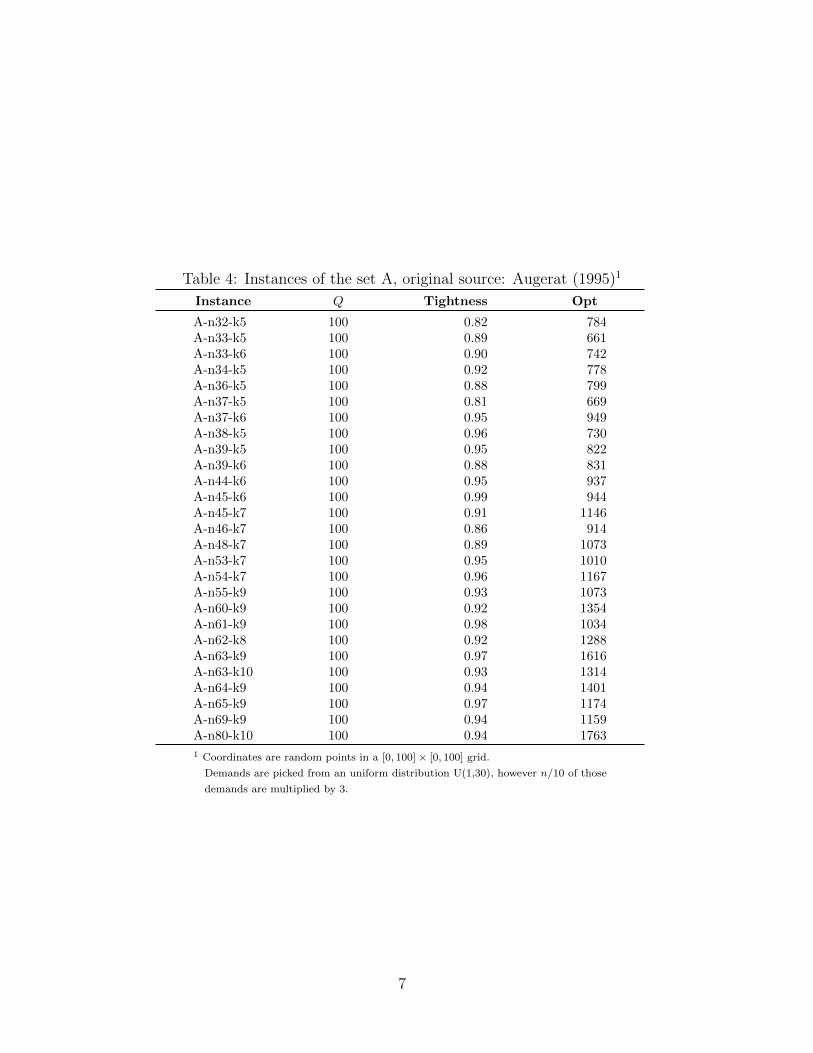
Table 4: Instances of the set A, original source: Augerat (1995)1
Instance Q Tightness Opt
A-n32-k5 100 0.82 784A-n33-k5 100 0.89 661A-n33-k6 100 0.90 742A-n34-k5 100 0.92 778A-n36-k5 100 0.88 799A-n37-k5 100 0.81 669A-n37-k6 100 0.95 949A-n38-k5 100 0.96 730A-n39-k5 100 0.95 822A-n39-k6 100 0.88 831A-n44-k6 100 0.95 937A-n45-k6 100 0.99 944A-n45-k7 100 0.91 1146A-n46-k7 100 0.86 914A-n48-k7 100 0.89 1073A-n53-k7 100 0.95 1010A-n54-k7 100 0.96 1167A-n55-k9 100 0.93 1073A-n60-k9 100 0.92 1354A-n61-k9 100 0.98 1034A-n62-k8 100 0.92 1288A-n63-k9 100 0.97 1616A-n63-k10 100 0.93 1314A-n64-k9 100 0.94 1401A-n65-k9 100 0.97 1174A-n69-k9 100 0.94 1159A-n80-k10 100 0.94 1763
1 Coordinates are random points in a [0, 100] × [0, 100] grid.
Demands are picked from an uniform distribution U(1,30), however n/10 of those
demands are multiplied by 3.
7
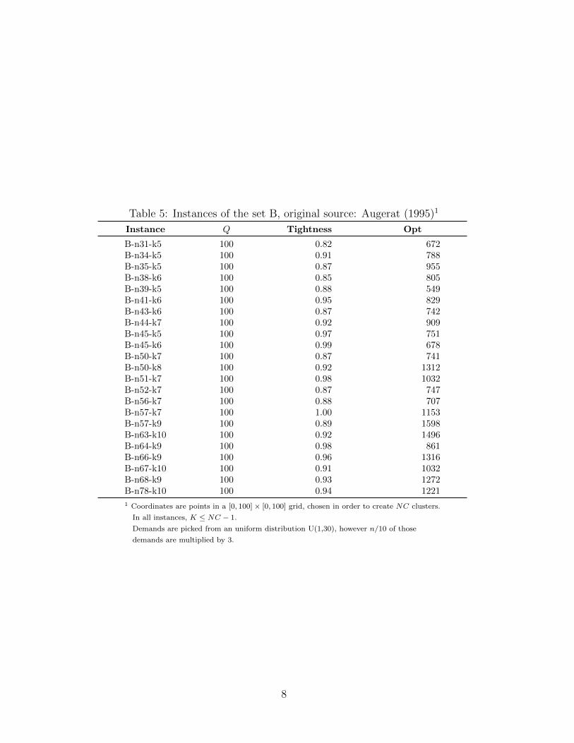
Table 5: Instances of the set B, original source: Augerat (1995)1
Instance Q Tightness Opt
B-n31-k5 100 0.82 672B-n34-k5 100 0.91 788B-n35-k5 100 0.87 955B-n38-k6 100 0.85 805B-n39-k5 100 0.88 549B-n41-k6 100 0.95 829B-n43-k6 100 0.87 742B-n44-k7 100 0.92 909B-n45-k5 100 0.97 751B-n45-k6 100 0.99 678B-n50-k7 100 0.87 741B-n50-k8 100 0.92 1312B-n51-k7 100 0.98 1032B-n52-k7 100 0.87 747B-n56-k7 100 0.88 707B-n57-k7 100 1.00 1153B-n57-k9 100 0.89 1598B-n63-k10 100 0.92 1496B-n64-k9 100 0.98 861B-n66-k9 100 0.96 1316B-n67-k10 100 0.91 1032B-n68-k9 100 0.93 1272B-n78-k10 100 0.94 1221
1 Coordinates are points in a [0, 100] × [0, 100] grid, chosen in order to create NC clusters.
In all instances, K ≤ NC − 1.
Demands are picked from an uniform distribution U(1,30), however n/10 of those
demands are multiplied by 3.
8

Table 6: Instances of the set P, original source: Augerat (1995)1
Instance Q Tightness Opt
P-n16-k8 35 0.88 450P-n19-k2 160 0.97 212P-n20-k2 160 0.97 216P-n21-k2 160 0.93 211P-n22-k2 160 0.96 216P-n22-k8 3000 0.94 603P-n23-k8 40 0.98 529P-n40-k5 140 0.88 458P-n45-k5 150 0.92 510P-n50-k7 150 0.91 554P-n50-k8 120 0.99 631P-n50-k10 100 0.95 696P-n51-k10 80 0.97 741P-n55-k7 170 0.88 568P-n55-k8 160 0.81 588P-n55-k10 115 0.91 694P-n55-k15 70 0.99 989P-n60-k10 120 0.95 744P-n60-k15 80 0.95 968P-n65-k10 130 0.94 792P-n70-k10 135 0.97 827P-n76-k4 350 0.97 593P-n76-k5 280 0.97 627P-n101-k4 400 0.91 681
1 Modifications in the capacity of some instances from A, B and E series.
Required number of routes are adjusted accordingly.
9
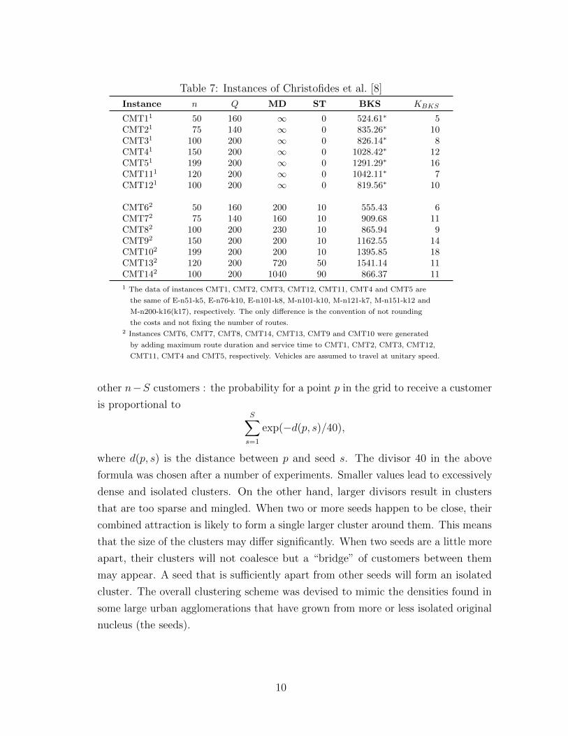
Table 7: Instances of Christofides et al. [8]
Instance n Q MD ST BKS KBKS
CMT11 50 160 ∞ 0 524.61∗ 5CMT21 75 140 ∞ 0 835.26∗ 10CMT31 100 200 ∞ 0 826.14∗ 8CMT41 150 200 ∞ 0 1028.42∗ 12CMT51 199 200 ∞ 0 1291.29∗ 16CMT111 120 200 ∞ 0 1042.11∗ 7CMT121 100 200 ∞ 0 819.56∗ 10
CMT62 50 160 200 10 555.43 6CMT72 75 140 160 10 909.68 11CMT82 100 200 230 10 865.94 9CMT92 150 200 200 10 1162.55 14CMT102 199 200 200 10 1395.85 18CMT132 120 200 720 50 1541.14 11CMT142 100 200 1040 90 866.37 11
1 The data of instances CMT1, CMT2, CMT3, CMT12, CMT11, CMT4 and CMT5 are
the same of E-n51-k5, E-n76-k10, E-n101-k8, M-n101-k10, M-n121-k7, M-n151-k12 and
M-n200-k16(k17), respectively. The only difference is the convention of not rounding
the costs and not fixing the number of routes.2 Instances CMT6, CMT7, CMT8, CMT14, CMT13, CMT9 and CMT10 were generated
by adding maximum route duration and service time to CMT1, CMT2, CMT3, CMT12,
CMT11, CMT4 and CMT5, respectively. Vehicles are assumed to travel at unitary speed.
other n−S customers : the probability for a point p in the grid to receive a customer
is proportional toS∑
s=1
exp(−d(p, s)/40),
where d(p, s) is the distance between p and seed s. The divisor 40 in the above
formula was chosen after a number of experiments. Smaller values lead to excessively
dense and isolated clusters. On the other hand, larger divisors result in clusters
that are too sparse and mingled. When two or more seeds happen to be close, their
combined attraction is likely to form a single larger cluster around them. This means
that the size of the clusters may differ significantly. When two seeds are a little more
apart, their clusters will not coalesce but a “bridge” of customers between them
may appear. A seed that is sufficiently apart from other seeds will form an isolated
cluster. The overall clustering scheme was devised to mimic the densities found in
some large urban agglomerations that have grown from more or less isolated original
nucleus (the seeds).
10
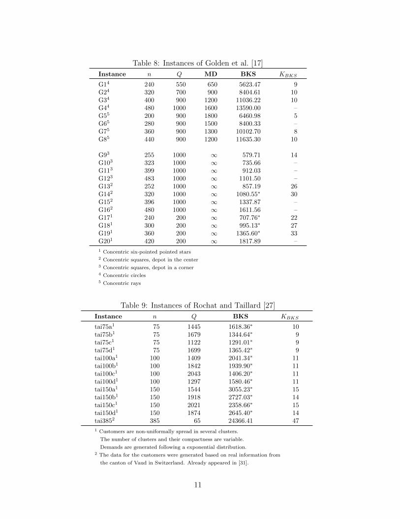
Table 8: Instances of Golden et al. [17]
Instance n Q MD BKS KBKS
G14 240 550 650 5623.47 9G24 320 700 900 8404.61 10G34 400 900 1200 11036.22 10G44 480 1000 1600 13590.00 –G55 200 900 1800 6460.98 5G65 280 900 1500 8400.33 –G75 360 900 1300 10102.70 8G85 440 900 1200 11635.30 10
G93 255 1000 ∞ 579.71 14G103 323 1000 ∞ 735.66 –G113 399 1000 ∞ 912.03 –G123 483 1000 ∞ 1101.50 –G132 252 1000 ∞ 857.19 26G142 320 1000 ∞ 1080.55∗ 30G152 396 1000 ∞ 1337.87 –G162 480 1000 ∞ 1611.56 –G171 240 200 ∞ 707.76∗ 22G181 300 200 ∞ 995.13∗ 27G191 360 200 ∞ 1365.60∗ 33G201 420 200 ∞ 1817.89 –
1 Concentric six-pointed pointed stars2 Concentric squares, depot in the center3 Concentric squares, depot in a corner4 Concentric circles5 Concentric rays
Table 9: Instances of Rochat and Taillard [27]
Instance n Q BKS KBKS
tai75a1 75 1445 1618.36∗ 10tai75b1 75 1679 1344.64∗ 9tai75c1 75 1122 1291.01∗ 9tai75d1 75 1699 1365.42∗ 9tai100a1 100 1409 2041.34∗ 11tai100b1 100 1842 1939.90∗ 11tai100c1 100 2043 1406.20∗ 11tai100d1 100 1297 1580.46∗ 11tai150a1 150 1544 3055.23∗ 15tai150b1 150 1918 2727.03∗ 14tai150c1 150 2021 2358.66∗ 15tai150d1 150 1874 2645.40∗ 14tai3852 385 65 24366.41 47
1 Customers are non-uniformally spread in several clusters.
The number of clusters and their compactness are variable.
Demands are generated following a exponential distribution.2 The data for the customers were generated based on real information from
the canton of Vaud in Switzerland. Already appeared in [31].
11

Table 10: Instances of Li et al. [19]1
Instance n Q MD BKS KBKS
21 560 1200 1800 16212.74 –22 600 900 1000 14499.04 1523 640 1400 2200 18801.12 1024 720 1500 2400 21389.33 –25 760 900 900 16668.51 1926 800 1700 2500 23971.74 –27 840 900 900 17343.38 2028 880 1800 2800 26565.92 –29 960 2000 3000 29154.33 –30 1040 2100 3200 31742.51 –31 1120 2300 3500 34330.84 –32 1200 2500 3600 37159.41 11
Random-Clustered (RC) – Half of the customers are clustered by the above
described scheme, the remaining customers are randomly positioned.
It should be noted that superpositions are not allowed, all customers and the depot
are located in distinct points on the grid.
3.1.3 Demand Distribution
Seven options of demand distributions have been selected in these instances.
Unitary (U) – All demands have value 1.
Small Values, Large Variance (1-10) – demands from UD[1,10].
Small Values, Small Variance (5-10) – demands from UD[5,10].
Large Values, Large Variance (1-100) – demands from UD[1,100].
Large Values, Small Variance (50-100) – demands from UD[50,100].
Depending on Quadrant (Q) – demands taken from UD[1,50] if customer is in
an even quadrant (with respect to point (500,500)), and from UD[51,100] otherwise.
This kind of demand distribution leads to solutions containing some routes that are
significantly longer (in terms of number of served customers) than others.
Many Small Values, Few Large Values (SL) – Most demands (70% to 95% of
the customers) are taken from UD[1,10], the remaining demands are taken from
UD[50,100].
12
3.1.4 Average Route Size
The previous experience of the authors with CVRP algorithms indicated that the value
n/Kmin, the average route size (assuming solutions with the minimum possible number
of routes) has a large impact on the performance of current exact methods. The impact
of this attribute on heuristic methods is not so pronounced, but is still quite significant.
We can not make a general statement that instances with shorter routes are easier than
instances with longer routes or the opposite. What happens is that some methods are more
suited for short routes and other methods for longer routes. Therefore, a comprehensive
benchmark set should contain instances where this attribute vary over a wide range of
values. Yet, generating an instance with exactly a given value of n/Kmin would be difficult,
since even computing Kmin requires the solution of a bin-packing problem. The generator
actually uses as attribute a value r representing the desired value of n/Kmin. This causes
the instance capacity to be defined as:
Q = dr∑n
i=1 qin
e,
where the q vector represents the demands, already obtained according to the specified
demand distribution. As∑n
i=1 qi/Q is usually a good lower bound on Kmin, instances
have values of n/Kmin that are sufficiently close to r.
3.2 Instance Generation
A benchmark set with instances corresponding to the cartesian product of so many
parameter values (even restricting the “continuous” parameters n and r to a reasonably
small number of values) would be huge. Thus, we generated a sample of 100 instances,
presented in Tables 11 to 13. We believe that this number of instances is large enough to
obtain the desired level of diversification, but still small enough to allow that future users
of the benchmark can report detailed results for each instance. We now explain how the
attribute values of those 100 instances were obtained.
• The instances are ordered by the number of customers n. For the first 50 instances,
ranging from 100 to 330 customers, n is increased in linear steps. For the last 50
instances, n is increased in exponential steps from 335 to 1000. For the time being,
instances with around 200 customers can already be hard for exact methods, and
larger instances are sufficiently challenging to highlight significant quality differences
between competing heuristics.
13

• The set of values of r were taken from a continuous triangular distribution T(3,6,25)
(minimum 3, mode 6 and maximum 25). The 100 values of r were partitioned in
quintiles, corresponding to very small routes, small routes, medium routes, long routes
and very long routes. The k-th instance receives an r from the ((k − 1) mod 5) + 1
quintile. In this way, it is guaranteed that every set containing 5t instances with
consecutive values of n will have exactly t instances from each quintile. It can
be observed in the end of Table 13 that the resulting set of n/Kmin values have
minimum 3.0, maximum 24.4, median 9.8 and average 11.1.
• A random permutation of the 3 possible values for the depot positioning attribute (C,
E and R) provides the values for the first 3 instances. Another random permutation
gives the values for the next 3 instances and so on. A similar scheme is used for
obtaining the values for the customer positioning and demand distribution attributes.
This guarantees that every subset of the instances with consecutive values of n will
have a near-balanced number of instances having the same value of an attribute.
The name of an instance follows the ABEFMP standard, and has a format X-nA-kB,
where A represents n+ 1, the number of points in the instance including the depot, and
B is the minimum possible number of routes Kmin, calculated by solving a bin-packing
problem. Since there are no two instances with the same number of points, in contexts
where the Kmin information is not considered much important, we propose the format XA
as an alternative shorter name. For example, the shorter name for X-n284-k15 would be
X284.
3.3 Two Decisions on Conventions
3.3.1 Rounding the Distances or Not?
Following the TSPLIB convention [26], the euclidean distances are rounded to the nearest
integer in the literature on exact methods. On the other hand, the distances are seldom
rounded in the literature on heuristics.
Advantages of Rounding – Most mathematical programming based algorithms
(including standard MIP solvers) have a limited optimality precision. For example, CPLEX
12.5 default precision is only 10−4 (0.01%). It is possible to increase the precision up
to a point by adjusting parameters (say, 10−6 or 10−7). Going further requires special
software, using more bits in the floating-point numbers or even exact rational arithmetic
[11], that is not easily available or implementable. The practice of distance rounding is
14
convenient for avoiding those pitfalls and usually makes the optimal values found by exact
methods based on standard mathematical programming software reliable. Remark that
the practice of not rounding, but only reporting two decimal places does not solve the
problem. For example, an algorithm with a precision of 10−6 may declare a solution having
value 853.2351 (published as 853.24) as optimal. Later, someone finds a solution with
value 853.2349 and publishes 853.23.
Disavantages of Rounding – A benchmark of rounded instances has less power for
comparing competing algorithms. Especially for heuristics, the search space is formed by
a relatively small number of plateaus, i.e., sets of solutions with the same value. Guiding
the search on such plateaus is usually done by trial and error since there is no indication
that the distance is –even slightly– reduced. There may also be in practice several distinct
optimal solutions, leading to more frequent ties between competitors. This effect is quite
significant on ABEFMP instances, where the optimal solution values have magnitudes
around 103. In addition, some people claim (but never publish, this is part of the commu-
nity folklore) that rounding can artificially enhance the performance of exact methods.
For example, if an upper bound of 1000 is known, a branch-and-bound node with lower
bound 999 +ε can be fathomed. This effect is significant on ABEFMP instances, enough
to make some algorithms to run at least twice as fast.
We took the decision that the newly proposed benchmark set will follow the TSPLIB
convention of rounding distances. Nevertheless, the instances were devised in order to
minimize the above mentioned disadvantages. The use of a [0, 1000]× [0, 1000] grid (instead
of the [0, 100]× [0, 100] grids of most ABEFMP instances) makes the optimal solutions
to have magnitudes between 104-105. This is still quite safe for exact methods having
a precision of 10−6. However, the plateau effect and the artificial enhancement of exact
methods are much reduced.
3.3.2 Fix the Number of Routes or Not?
The literature on exact methods usually follows the convention of fixing the number of
routes to a value K. Except for instance M-n200-k17, K is always set to Kmin. The
standard explanation for that fixing is that K represents the number of vehicles available
at the depot. A more sophisticated explanation is that fixing the number of routes to the
minimum is an indirect way of minimizing the fixed costs for using a vehicle. We do not
think that this is necessarily true : since the CVRP definition allows solutions containing
routes that are much shorter than others, why not assigning the two shortest routes to
15
the same vehicle? In fact, the CVRP may be used to model real-world situations where a
single vehicle (a truly homogeneous fleet!) will perform all routes in sequence. In other
words, CVRP routes do not need to correspond to vehicles. Based on that reasoning, we
decided that the newly proposed benchmark set will follow the convention of not fixing
the number of routes. Therefore, the number Kmin indicated in each instance should be
taken only as a lower bound on the number of routes in a solution. A second reason for
taking that decision is that the number of routes was not fixed in the original CVRP
definition [12].
4 Experiments with State-of-the-Art Methods
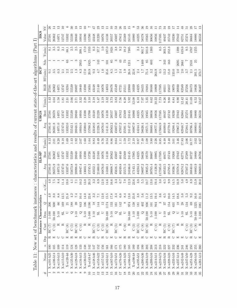
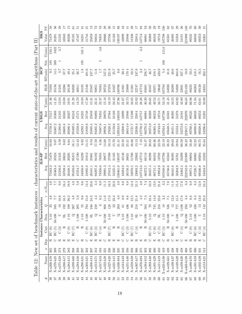
In order to provide an initial set of results to the new benchmark, experiments have been
conducted with recent state-of-the-art heuristic and exact methods. The experiments
also provide an assessment of the level of difficulty of the proposed instances and even
some hints on how the attributes used in their generation impact on that difficulty. Those
results are reported jointly in Tables 11 to 13, which describe the characteristics of each
instance, the average solution quality, best solutions quality and average CPU time of
two state-of-the-art metaheuristics, the lower bound, root CPU time, number of search
nodes and overall time of a recent state-of-the-art exact method, and finally the cost and
number of vehicles of the best solution (BKS) ever found since the instances were created,
including preliminary runs of those heuristics with alternative parameterizations. Table
13 also reports additional statistics on instances characteristics and results, such as the
minimum, maximum, average and median results on the instance set for n, Q, r, n/Kmin,
as well as for the Gaps(%) and CPU time of ILS-SP, UHGS and BCP (root relaxation).
4.1 Heuristic solutions
We selected a pair of recent successful metaheuristics to illustrate the two main current
types of approaches in the literature. We consider an efficient neighborhood-based method,
the iterated local search based matheuristic algorithm (ILS-SP) of Subramanian et al. [30],
and a recent population-based method, the unified hybrid genetic search (UHGS) of Vidal
et al. [32, 33]. These two methods rely extensively on local search to improve new solutions
generated either by shaking or recombinations of parents. They also include specific
strategies to explore new choices of customer-to-route assignments: ILS is coupled with a
integer programming solver over a set partitioning (SP) formulation, which seeks to create
new solutions based on known routes from past local optimums, while UHGS implements
16
Tab
le11
:N
ewse
tof
ben
chm
ark
inst
ance
s:
char
acte
rist
ics
and
resu
lts
ofcu
rren
tst
ate-
of-t
he-
art
algo
rith
ms
(Par
tI)
InstanceChara
cteristics
ILS-S
PUHGS
BCP
BKS
#N
am
en
Dep
Cu
stD
emQ
rn/K
min
Avg
Bes
tT
(min
)A
vg
Bes
tT
(min
)R
LB
RT
(min
)N
ds
T(m
in)
Val
ue
NV
1X
-n101
-k25
100
RR
C(7
)1-
100
206
4.0
4.0
275
91.0
27591
0.13
275
91.
027
591
1.43
2759
10.1
10.1
275
9126
2X
-n106
-k14
105
EC
(3)
50-
100
600
8.0
7.5
263
75.9
26362
2.01
263
81.
826
378
4.04
2636
23.5
13.5
263
6214
3X
-n110
-k13
109
CR
5-10
668.
88.
4149
71.0
14971
0.20
149
71.
014
971
1.58
1497
10.3
10.3
149
7113
4X
-n115
-k10
114
CR
SL
169
12.
511.
4127
47.0
12747
0.18
127
47.
012
747
1.81
1274
72.1
12.1
127
4710
5X
-n12
0-k
611
9E
RC
(8)
U21
21.8
19.8
133
37.6
13332
1.69
133
32.
013
332
2.31
1323
42.2
63
88.1
133
326
6X
-n125
-k30
124
RC
(5)
Q188
4.2
4.1
556
73.8
55539
1.43
555
42.
155
539
2.66
5553
92.5
12.5
555
3930
7X
-n129
-k18
128
ER
C(8
)1-
1039
7.4
7.1
289
98.0
28948
1.92
289
48.
528
940
2.71
2889
71.3
32.5
289
4018
8X
-n134
-k13
133
RC
(4)
Q643
10.
410
.2109
47.4
10916
2.07
109
34.
910
916
3.32
1084
08.3
295
539
9.1
109
1613
9X
-n139
-k10
138
CR
5-10
106
14.0
13.
8136
03.1
13590
1.60
135
90.
013
590
2.28
1359
017
.01
17.0
135
9010
10X
-n143
-k7
142
ER
1-1
00119
022
.620
.3157
45.2
15726
1.64
157
00.
215
700
3.10
1563
420
.9182
51553
157
007
11X
-n14
8-k46
147
RR
C(7
)1-1
018
3.2
3.2
434
52.1
43448
0.84
434
48.
043
448
3.18
4344
80.3
10.3
434
4847
12X
-n15
3-k22
152
CC
(3)
SL
144
7.1
6.9
214
00.0
21340
0.49
212
26.
321
220
5.47
2114
04.7
143
37.7
212
2023
13X
-n15
7-k13
156
RC
(3)
U12
12.
012
.0168
76.0
16876
0.76
168
76.
016
876
3.19
1687
61.0
11.0
168
7613
14X
-n16
2-k11
161
CR
C(8
)50
-100
1174
15.5
14.
6141
60.1
14138
0.54
141
41.
314
138
3.32
1405
335
.610
118
7.0
141
3811
15X
-n16
7-k10
166
ER
5-10
133
17.8
16.6
206
08.7
20562
0.86
205
63.
220
557
3.73
2047
68.5
85
1024
205
5710
16X
-n17
2-k51
171
CR
C(5
)Q
161
3.4
3.4
456
16.1
45607
0.64
456
07.
045
607
3.83
4554
91.5
33.8
456
0753
17X
-n17
6-k26
175
ER
SL
142
6.8
6.7
482
49.8
48140
1.11
479
57.
247
812
7.56
4772
12.4
43
9.2
478
1226
18X
-n18
1-k23
180
RC
(6)
U8
8.4
7.8
255
71.5
25569
1.59
255
91.
125
569
6.28
2551
11.9
73
18.2
255
6923
19X
-n18
6-k15
185
RR
50-1
00974
13.
012
.3241
86.0
24145
1.72
241
47.
224
145
5.92
2398
026
.8121
17305
241
4515
20X
-n190
-k8
189
EC
(3)
1-10
138
25.
023
.6171
43.1
17085
2.10
169
87.
916
980
12.
0816
939
22.8
169
808
21X
-n19
5-k51
194
CR
C(5
)1-1
00
181
3.8
3.8
442
34.3
44225
0.87
442
44.
144
225
6.10
4422
52.4
12.4
442
2553
22X
-n20
0-k36
199
RC
(8)
Q402
5.6
5.5
586
97.2
58626
7.48
586
26.
458
578
7.97
5845
51.7
146
990
1.7
585
7836
23X
-n20
4-k19
203
CR
C(6
)50
-100
836
11.2
10.7
196
25.2
19570
1.08
195
71.
519
565
5.35
1948
475
.485
501.6
195
6519
24X
-n20
9-k16
208
ER
5-10
101
13.5
13.0
307
65.4
30667
3.80
306
80.
430
656
8.62
3048
03.2
603
1303
306
5616
25X
-n21
4-k11
213
CC
(4)
1-10
0944
19.4
19.4
111
26.9
10985
2.26
108
77.
410
856
10.
2210
809
264
.9108
5611
26X
-n21
9-k73
218
ER
U3
3.6
3.0
117
595
.011
759
50.
85
11760
4.9
1175
957.7
311
759
50.5
10.5
1175
95
73
27
X-n
223
-k34
222
RR
C(5
)1-1
037
6.5
6.5
405
33.5
40471
8.48
404
99.
040
437
8.26
4031
113
.234
330
3.5
404
3734
28X
-n22
8-k23
227
RC
(8)
SL
154
10.0
9.9
257
95.8
25743
2.40
257
79.
325
742
9.80
2565
715
.016
325
2.3
257
4223
29X
-n23
3-k16
232
CR
C(7
)Q
631
14.
514
.5193
36.7
19266
3.01
192
88.
419
230
6.84
1907
0133
.0192
3017
30X
-n23
7-k14
236
ER
U18
18.6
16.9
270
78.8
27042
3.46
270
67.
327
042
8.90
2693
02.0
269
513
98270
4214
31X
-n24
2-k48
241
ER
1-10
28
5.0
5.0
828
74.2
82774
17.
83829
48.
782
804
12.
4282
589
2.0
266
181
9.0
827
5148
32X
-n24
7-k50
246
CC
(4)
SL
134
5.3
4.9
375
07.2
37289
2.06
372
84.
437
274
20.
4137
256
3.7
79.5
372
7451
33X
-n25
1-k28
250
RR
C(3
)5-1
069
9.2
8.9
388
40.0
38727
10.
77387
96.
438
699
11.
6938
473
2.1
253
147
67386
8428
34X
-n25
6-k16
255
CC
(8)
50-
100
1225
16.
015
.9188
83.9
18880
2.02
188
80.
018
880
6.52
1882
6201
.525
1255
188
8017
35X
-n26
1-k13
260
ER
1-1
00108
121
.020
.0268
69.0
26706
6.67
266
29.
626
558
12.
6726
407
373
.7265
5813
17
Tab
le12
:N
ewse
tof
ben
chm
ark
inst
ance
s:
char
acte
rist
ics
and
resu
lts
ofcu
rren
tst
ate-
of-t
he-
art
algo
rith
ms
(Par
tII
)In
stanceChara
cteristics
ILS-S
PUHGS
BCP
BKS
#N
ame
nD
epC
ust
Dem
Qr
n/K
min
Avg
Bes
tT
(min
)A
vg
Bes
tT
(min
)R
LB
RT
(min
)N
ds
T(m
in)
Valu
eN
V
36X
-n26
6-k
5826
5R
RC
(6)
5-1
035
4.6
4.6
7556
3.3
754
78
10.0
375
759
.37551
721.
36753
50
9.5
185
150
.1754
78
58
37
X-n
270-
k35
269
CR
C(5
)50
-100
585
7.7
7.7
3536
3.4
353
24
9.0
735
367
.23530
311.
25351
56
14.
538
934
22
352
91
36
38
X-n
275-
k28
274
RC
(3)
U10
10.8
9.8
2125
6.0
212
45
3.5
921
280
.62124
512.
04212
45
3.7
13.7
212
45
28
39
X-n
280-
k17
279
ER
SL
192
16.5
16.
433
769.4
336
24
9.6
233
605
.83350
519.
09332
86
87.
7335
03
17
40
X-n
284-
k15
283
RC
(8)
1-10
109
20.2
18.9
2044
8.5
202
95
8.6
420
286
.42022
719.
91201
39
49.
4202
26
15
41
X-n
289-
k60
288
ER
C(7
)Q
267
4.8
4.8
9545
0.6
953
15
16.1
195
469
.59524
421.
28949
28
25.
1951
85
61
42
X-n
294-
k50
293
CR
1-10
028
55.9
5.9
4725
4.7
471
90
12.4
247
259
.04717
114.
70469
11
26.
7471
67
51
43
X-n
298-
k31
297
RR
1-10
559.
69.
634
356.0
342
39
6.9
234
292
.13423
110.
93341
05
1.8
195
531
.1342
31
31
44
X-n
303-
k21
302
CC
(8)
1-10
0794
15.0
14.4
2189
5.8
218
12
14.1
521
850
.92174
817.
28215
46
481.
0217
44
21
45
X-n
308-
k13
307
ER
C(6
)S
L24
624
.223.
626
101.1
259
01
9.5
325
895
.42585
915.
31255
87
247.
7258
59
13
46
X-n
313-
k71
312
RR
C(3
)Q
248
4.4
4.4
9429
7.3
941
92
17.5
094
265
.29409
322.
41938
51
11.
6940
44
72
47
X-n
317-
k53
316
EC
(4)
U6
6.2
6.0
7835
6.0
783
55
8.5
678
387
.87835
522.
37783
34
1.7
54.6
783
55
53
48
X-n
322-
k28
321
CR
50-1
00
868
11.6
11.
529
991.3
298
77
14.6
829
956
.12987
015.
16297
22
547.
2298
66
28
49
X-n
327-
k20
326
RR
C(7
)5-1
0128
17.0
16.3
2781
2.4
275
99
19.1
327
628
.22756
418.
19273
78
221.
9275
56
20
50
X-n
331-
k15
330
ER
U23
23.
422
.031
235.5
311
05
15.7
031
159
.63110
324.
43310
27
25.
7311
03
15
51
X-n
336-
k84
335
ER
Q20
34.
04.
0139
461.0
1391
97
21.4
1139
534
.913
921
037
.96
1387
06
6.6
1391
97
86
52X
-n344
-k43
343
CR
C(7
)5-
1061
8.0
8.0
4228
4.0
421
46
22.5
842
208
.84209
921.
67418
81
20.
4420
99
43
53
X-n
351-
k40
350
CC
(3)
1-10
0436
8.8
8.8
2615
0.3
260
21
25.2
126
014
.02594
633.
73258
09
170.
4259
46
41
54
X-n
359-
k29
358
ER
C(7
)1-
1068
12.5
12.3
5207
6.5
517
06
48.8
651
721
.75150
934.
85513
81
82.
3515
09
29
55
X-n
367-
k17
366
RC
(4)
SL
218
21.
821
.523
003.2
229
02
13.1
322
838
.42281
422.
02227
47
247.
9228
14
17
56
X-n
376-
k94
375
ER
U4
4.2
4.0
147
713.0
1477
13
7.1
0147
750
.214
771
728
.26
1477
13
3.3
13.3
1477
13
94
57X
-n384
-k52
383
RR
50-
100
564
7.4
7.4
6637
2.5
661
16
34.4
766
270
.26608
140.
20656
81
256.
7660
81
53
58
X-n
393-
k38
392
CR
C(5
)5-
1078
10.4
10.3
3845
7.4
382
98
20.8
238
374
.93826
928.
65381
67
46.
7382
69
38
59
X-n
401-
k29
400
EC
(6)
Q74
514
.013
.866
715.1
664
53
60.3
666
365
.46624
349.
52659
71
318.
1662
43
29
60
X-n
411-
k19
410
RC
(5)
SL
216
22.
621
.619
954.9
197
92
23.7
619
743
.81971
834.
71196
40
433.
9197
18
19
61
X-n
420
-k13
041
9C
RC
(3)
1-10
18
3.2
3.2
107
838.0
1077
98
22.1
9107
924
.110
779
853
.19
1077
04
5.4
169
115
.01077
98
130
62X
-n429
-k61
428
RR
50-
100
536
7.1
7.0
6574
6.6
655
63
38.2
265
648
.56550
141.
45649
30
31.
6655
01
62
63
X-n
439-
k37
438
CR
C(8
)U
1212
.011
.836
441.6
363
95
39.6
336
451
.13639
534.
55362
89
20.
0363
95
37
64
X-n
449-
k29
448
ER
1-1
0077
715.
515
.456
204.9
557
61
59.9
455
553
.15537
864.
92549
28
804.
9553
58
29
65
X-n
459-
k26
458
CC
(4)
Q1106
17.8
17.6
2446
2.4
242
09
60.5
924
272
.62418
142.
80239
31
327.
1241
81
26
66
X-n
469
-k13
846
8E
R50
-100
256
3.4
3.4
222
182.0
2219
09
36.3
2222
617
.122
207
086
.65
2214
29
10.9
2219
09
140
67X
-n480
-k70
479
RC
(8)
5-10
526.
86.
889
871.2
896
94
50.4
089
760
.18953
566.
96892
35
59.
5895
35
70
68
X-n
491-
k59
490
RR
C(6
)1-
100
428
8.4
8.3
6722
6.7
669
65
52.2
366
898
.06663
371.
94662
63
418.
1666
33
60
69
X-n
502-
k39
501
EC
(3)
U13
13.0
12.
869
346.8
692
84
80.7
569
328
.86925
363.
61691
20
16.
5692
53
39
70
X-n
513-
k21
512
CR
C(4
)1-
10142
25.0
24.4
2443
4.0
243
32
35.0
424
296
.62420
133.
09240
53
262.
1242
01
21
18

Tab
le13
:N
ewse
tof
ben
chm
ark
inst
ance
s:
char
acte
rist
ics
and
resu
lts
ofcu
rren
tst
ate-
of-t
he-
art
algo
rith
ms
(Par
tII
I)In
stanceChara
cteristics
ILS-S
PUHGS
BCP
BKS
#N
ame
nD
epC
ust
Dem
Qr
n/K
min
Avg
Bes
tT
(min
)A
vg
Bes
tT
(min
)R
LB
RT
(min
)N
ds
T(m
in)
Valu
eN
V
70
X-n
513
-k21
512
CR
C(4
)1-
10
142
25.0
24.
4244
34.
024
332
35.
042429
6.6
242
01
33.0
924
053
262
.12420
121
71
X-n
524-k
153
523
RR
SL
125
3.8
3.4
1550
05.0
154
709
27.
2715
497
9.5
1547
7480.7
0154
533
12.5
381
212.
115
459
4155
72
X-n
536-
k96
535
CC
(7)
Q371
5.6
5.6
957
00.
795
524
62.
079533
0.6
951
22
107.5
394
409
47.9
9512
297
73
X-n
548-
k50
547
ER
U11
11.2
10.9
868
74.
186
710
63.
958699
8.5
868
22
84.2
486
604
16.1
8671
050
74
X-n
561-
k42
560
CR
C(7
)1-
10
7413
.513
.3431
31.
342
952
68.
864286
6.4
427
56
60.6
042
495
302
.34275
642
75
X-n
573-
k30
572
EC
(3)
SL
210
19.4
19.1
511
73.
051
092
112.
035091
5.1
507
80
188.1
550
575
1306
.95078
030
76
X-n
586-k
159
585
RR
C(4
)5-1
028
3.6
3.7
1909
19.0
190
612
78.
5419
083
8.0
1905
4317
5.2
9189
950
7.1
19054
3159
77
X-n
599-
k92
598
RR
50-
100
487
6.5
6.5
1093
84.0
109
056
72.
9610
906
4.2
1088
1312
5.9
1108
000
264
.310
881
394
78
X-n
613-
k62
612
CR
1-10
052
310
.09.9
604
44.
260
229
74.
805996
0.0
597
78
117.3
159
323
1429
.85977
862
79
X-n
627-
k43
626
EC
(5)
5-1
011
014
.514
.6629
05.
662
783
162.
676252
4.1
623
66
239.6
862
018
600
.26236
643
80
X-n
641-
k35
640
ER
C(8
)50-
100
138
118
.618.
3646
06.
164
462
140.
426419
2.0
638
39
158.8
163
228
401
.06383
935
81
X-n
655-k
131
654
CC
(4)
U5
5.0
5.0
1067
82.0
106
780
47.
2410
689
9.1
1068
2915
0.4
8106
766
8.5
21
41.5
10678
0131
82
X-n
670-k
130
669
RR
SL
129
5.3
5.1
1476
76.0
147
045
61.
2414
722
2.7
1467
0526
4.1
0146
211
103
.114
670
5134
83
X-n
685-
k75
684
CR
C(6
)Q
408
9.2
9.1
689
88.
268
646
73.
856865
4.1
684
25
156.7
167
925
1643
.26842
575
84
X-n
701-
k44
700
ER
C(7
)1-
1087
16.0
15.9
830
42.
282
888
210.
088248
7.4
822
93
253.1
781
694
680
.68229
244
85
X-n
716-
k35
715
RC
(3)
1-10
010
0721
.020
.4441
71.
644
021
225.
794364
1.4
435
25
264.2
843
113
419
.54352
535
86
X-n
733-k
159
732
CR
1-1
025
4.6
4.6
1370
45.0
136
832
111.
5613
658
7.6
1363
6624
4.5
3135
748
57.9
13636
6160
87
X-n
749-
k98
748
RC
(8)
1-10
0396
7.7
7.6
782
75.
977
952
127.
247786
4.9
777
15
313.8
876
924
259
.27770
098
88
X-n
766-
k71
765
ER
C(7
)S
L166
10.8
10.8
1157
38.0
115
443
242.
1111
514
7.9
1146
8338
2.9
9114
108
262
.811
468
371
89
X-n
783-
k48
782
RR
Q83
216
.516.
3737
22.
973
447
235.
487300
9.6
727
81
269.7
071
728
332
.87272
748
90
X-n
801-
k40
800
ER
U20
20.2
20.0
740
05.
773
830
432.
647373
1.0
735
87
289.2
473
124
258
.07358
740
91
X-n
819-k
171
818
CC
(6)
50-1
00
358
4.8
4.8
1594
25.0
159
164
148.
9115
889
9.3
1586
1137
4.2
8157
627
257
.215
861
1173
92
X-n
837-k
142
836
RR
C(7
)5-1
044
5.9
5.9
1950
27.0
194
804
173.
1719
447
6.5
1942
6646
3.3
6193
245
253
.719
426
6142
93
X-n
856-
k95
855
CR
C(3
)U
99.
69.0
892
77.
689
060
153.
658923
8.7
891
18
288.4
388
839
43.6
8906
095
94
X-n
876-
k59
875
EC
(5)
1-10
076
415
.014
.81004
17.0
100
177
409.
319988
4.1
997
15
495.3
898
880
433
.29971
559
95
X-n
895-
k37
894
RR
50-
100
181
624.
224.
2549
58.
554
713
410.
175443
9.8
541
72
321.8
953
147
984
.55417
238
96
X-n
916-k
207
915
ER
C(6
)5-
1033
4.4
4.4
3309
48.0
330
639
226.
0833
019
8.3
3298
3656
0.8
1328
588
97.1
32983
6208
97
X-n
936-k
151
935
CR
SL
138
6.2
6.2
1345
30.0
133
592
202.
5013
351
2.9
1331
4053
1.5
0132
496
395
.813
310
5159
98
X-n
957-
k87
956
RR
C(4
)U
1111
.611
.0859
36.
685
697
311.
208582
2.6
856
72
432.9
085
328
257
.18567
287
99
X-n
979-
k58
978
EC
(6)
Q99
817.
016
.91202
53.0
119
994
687.
2211
950
2.1
1191
9455
3.9
6118
399
937
.511
919
458
100
X-n
1001
-k43
1000
RR
–1-1
0131
23.4
23.3
739
85.
473
776
792.
757295
6.0
727
42
549.0
371
812
308
.87274
243
Min
100
33.
23.0
0.0
0%0.0
0%0.1
30.
00%
0.0
0%
1.43
0.0
0%0.1
Max
1000
181
625
.024
.42.5
0%1.4
2%792
.75
0.55
%0.1
3%
560.
811.8
9%164
3.2
Avg.
412
.2324
.611.
411.
10.5
2%0.2
5%71
.71
0.19
%0.0
1%
98.
790.4
4%18
9.4
Med
ian
333
149
10.2
9.9
0.3
8%0.1
0%17
.67
0.20
%0.0
0%
22.
390.4
0%33.6
19
a continuous diversification procedure by modifying the objective during parents and
survivors selection to promote not only good but also diverse solutions. Both methods are
known to achieve very high quality results on the previous sets of CVRP instances as well
as on various other vehicle routing variants.
The two methods have been run with the same parameter setting specified in the
original papers. To produce solutions that can stand the test of time, and counting on the
fact that more computing power will be surely available in the coming years, we selected
a slightly larger termination criterion for UHGS by allowing up to 50.000 consecutive
iterations without improvement. These tests have been conducted on a Xeon CPU with
3.07 GHz and 16 GB of RAM, running under Oracle Linux Server 6.4. The average and
best results on 50 runs are reported in the Table, as well as the average computational
time per instance.
From these tests, it appears that both ILS-SP and UHGS produce solutions of consistent
quality, with an average gap of 0.52% and 0.19%, respectively, with respect to the best
known solutions (BKS) ever found during all experiments. Considering the subset of
instances that are solved to optimality (see Section 4.2), ILS-SP and UHGS achieve average
gaps of 0.18% and 0.09%, respectively. A direct comparison of the best solutions found by
each method provides the following score: UHGS solutions are better 58 times, ILS-SP
solutions are better 9 times and there are 33 ties.
UHGS produces solutions of generally higher quality than ILS for a comparable amount
of CPU time, except for some instances containing few customers per route. For this
type of problems, the set partitioning solver can produce new high-quality solutions from
existing routes in a very efficient manner, while generating new structurally different
solutions with other choices of assignments is more challenging for local searches and
even for randomized crossovers. On the other hand, for problems with a large number of
customers per route, the hybrid ILS exhibits a slower convergence and generally leads to
solutions of lower quality.
Overall, these experiments show that some state-of-the-art methods may perform well
on different classes of instances. Therefore, a promising research path would involve the
extension of these methods and/or further hybridizations to cover all problems in the best
possible way.
4.2 Exact solutions
The Branch-Cut-and-Price (BCP) in Pecin et al. [22] is a complex algorithm that combines
and improves several ideas proposed by other authors [4, 5, 10, 28], as also detailed in [23].
20

The algorithm was run in a single core of an Intel i7-3960X 3.30GHz processor with 64
GB RAM. The value of the best solution found by the previously mentioned heuristics
was inputted as an initial upper bound. Actually, in order to increase our confidence in
the correctness of the implementation, we always add 1 to that upper bound. In this way,
the BCP always has to find by itself a feasible solution with value at least as good as the
upper bound.
The BCP could solve 40 out of the 100 new instances to optimality in reasonable times
(maximum of 5 days, for X-n186-k15). For those instances we report the root node lower
bound, the time to obtain that bound, the number of nodes in the search tree and the total
time. For the remaining 60 instances we only report a lower bound and the corresponding
time.
• The BCP can solve most instances with up to 275 customers. In the 38 instances
in that range, it only failed when the routes are very long (X-n190-k8, X-n214-k11,
X-n233-k16, and X-n261-k13). On the other hand, only 6 larger instances could
be solved (X-n298-k31, X-n317-k53, X-376-k94, X-n420-k130, X-n524-k153, and
X-nX655-k131). Those more favorable instances have short routes and small values
of Q.
• The BCP attested the general good quality of the solutions that can be found by
current heuristics. Consider the best solution provided either by ILS-SP or UHGS.
In 96 out of the 100 instances, this solution is less than 1% above the computed
lower bounds.
5 The CVRPLIB Web Site
The typical instance repository of today is a web page that allows downloading the instance
files and includes additional textual information, like file format description, instance
source, best known/optimal solution values, etc. The CVRLIB web page, where the new
instances (and all the previous CVRP instances described in Section 2) are available
(http://vrp.galgos.inf.puc-rio.br/index.php/en/), is more sophisticated:
• Its core is a full-fledged database containing, for each instance: (i) its actual data,
like n, Q, customer coordinates and demands, (ii) its best known/optimal solution,
represented as set of routes, (iii) a miscellanea of additional information, like original
source, the values of the attributes used in its generation (for the new instances), and
even comments about remarkable characteristics. The visible pieces of information
21

that appear in the web site are produced by queries. The objective of that design is
having a larger degree of consistency and flexibility in the maintenance of the page.
• The best known solutions are automatically verified, their feasibility is checked
and their costs are calculated from the original instance data. This eliminates the
possibility that false best known solutions appear due to typos or misunderstandings
about the conventions.
• Instances with euclidean distances (the vast majority) can be depicted graphically,
along with their best known/optimal solutions.
6 Conclusions
We hope that the proposed set of instances will contribute to spark new interest on the
“classic” CVRP, helping to test new algorithmic developments in the coming years. In
particular, by proposing a common set of benchmark instances for both heuristic and
exact methods, this work contributes to end a bizarre situation where minor convention
details were sufficient for isolating both communities. For example, most of the CVRP
instances in Table 7 could have their best known solutions proven to be optimal by the
algorithms in [4, 5, 10, 14, 28]. But none of those authors effectively changed a few lines
of code to adapt for the different conventions. This instance-induced isolation was harmful
and prevented a more effective cross-fertilization between exact and heuristic methods.
In fact, this paper has shown that it is already possible to perform direct comparisons
of heuristic results with good lower bounds or even proven optimal solutions on fairly
large-sized instances.
A major concern in the design of the new benchmark set was problem diversity. By
having instances covering a wider set of characteristics, the benchmark will favor the
development of more flexible methods (perhaps hybrids), that will eventually be applied
to real-life situations with lesser risks of failure due to an uncommon instance type.
Finally, we point out that the proposed CVRP instances can be extended to other clas-
sical VRP variants as needed, by providing additional data fields like duration constraints,
time windows, or heterogeneous fleet specifications.
22
Acknowledgments
The authors would like to thank Teobaldo Bulhoes Jr. for computing the values of Kmin
for the new set of proposed instances and Ivan Xavier de Lima for his help on creating the
CVRPLIB web page.
References
[1] Achuthan, N., Caccetta, L., Hill, S., 2003. An improved branch-and-cut algorithm for
the capacitated vehicle routing problem. Transportation Science 37, 153–169.
[2] Araque, J., Kudva, G., Morin, T., Pekny, J., 1994. A branch-and-cut algorithm for
the vehicle routing problem. Annals of Operations Research 50, 37–59.
[3] Augerat, P., Belenguer, J., Benavent, E., Corberan, A., Naddef, D., Rinaldi, G., 1995.
Computational results with a branch and cut code for the capacitated vehicle routing
problem. Tech. Rep. 949-M, Universite Joseph Fourier, Grenoble, France.
[4] Baldacci, R., Christofides, N., Mingozzi, A., 2008. An exact algorithm for the vehicle
routing problem based on the set partitioning formulation with additional cuts.
Mathematical Programming 115 (2), 351–385.
[5] Baldacci, R., Mingozzi, A., Roberti, R., 2011. New route relaxation and pricing
strategies for the vehicle routing problem. Operations Research 59 (5), 1269–1283.
[6] Blasum, U., Hochstattler, W., 2000. Application of the branch and cut method to
the vehicle routing problem. Tech. Rep. ZPR2000-386, Zentrum fur Angewandte
Informatik Koln.
[7] Christofides, N., Eilon, S., 1969. An algorithm for the vehicle-dispatching problem.
Operational Research Quarterly 20, 309–318.
[8] Christofides, N., Mingozzi, A., Toth, P., 1979. The vehicle routing problem. In:
Christofides, N., Mingozzi, A., Toth, P., Sandi, C. (Eds.), Combinatorial Optimization.
Vol. 1. Wiley Interscience, pp. 315–338.
[9] Clarke, G., Wright, J., 1964. Scheduling of vehicles from a central depot to a number
of delivery points. Operations research 12 (4), 568–581.
23
[10] Contardo, C., Martinelli, R., 2014. A new exact algorithm for the multi-depot vehicle
routing problem under capacity and route length constraints. Discrete Optimization
12, 129–146.
[11] Cook, W., Koch, T., Steffy, D. E., Wolter, K., 2011. An exact rational mixed-integer
programming solver. In: Integer Programming and Combinatoral Optimization.
Springer, pp. 104–116.
[12] Dantzig, G. B., Ramser, J. H., 1959. The truck dispatching problem. Management
science 6 (1), 80–91.
[13] Fisher, M., 1994. Optimal solution of vehicle routing problems using minimum K-trees.
Operations research 42 (4), 626–642.
[14] Fukasawa, R., Longo, H., Lysgaard, J., Poggi de Aragao, M., Reis, M., Uchoa,
E., Werneck, R., 2006. Robust branch-and-cut-and-price for the capacitated vehicle
routing problem. Mathematical programming 106 (3), 491–511.
[15] Gaskell, T., 1967. Bases for vehicle fleet scheduling. OR, 281–295.
[16] Gillett, B. E., Miller, L. R., 1974. A heuristic algorithm for the vehicle-dispatch
problem. Operations research 22 (2), 340–349.
[17] Golden, B., Wasil, E., Kelly, J., Chao, I., 1998. The impact of metaheuristics on
solving the vehicle routing problem: algorithms, problem sets, and computational
results. In: Fleet management and logistics. Springer, pp. 33–56.
[18] Gouveia, L., 1996. Multicommodity flow models for spanning trees with hop con-
straints. European Journal of Operational Research 95 (1), 178–190.
[19] Li, F., Golden, B., Wasil, E., 2005. Very large-scale vehicle routing: new test problems,
algorithms, and results. Computers & Operations Research 32 (5), 1165–1179.
[20] Lysgaard, J., Letchford, A., Eglese, R., 2004. A new branch-and-cut algorithm for
the capacitated vehicle routing problem. Mathematical Programming 100, 423–445.
[21] Nagata, Y., Braysy, O., 2009. Edge assembly-based memetic algorithm for the
capacitated vehicle routing problem. Networks 54 (4), 205–215.
[22] Pecin, D., Pessoa, A., Poggi, M., Uchoa, E., 2014. Improved branch-cut-and-price for
capacitated vehicle routing. In: Integer Programming and Combinatorial Optimization.
Springer, pp. 393–403.
24
[23] Poggi, M., Uchoa, E., 2014. New exact approaches for the capacitated VRP. In: Toth,
P., Vigo, D. (Eds.), Vehicle Routing: Problems, Methods, and Applications,. SIAM,
Ch. 3, pp. 59–86.
[24] Ralphs, T., Kopman, L., Pulleyblank, W., Jr., L. T., 2003. On the capacitated vehicle
routing problem. Mathematical Programming 94, 343–359.
[25] Rand, G. K., 2009. The life and times of the Savings Method for vehicle routing
problems. ORiON: The Journal of ORSSA 25 (2), 125–145.
[26] Reinelt, G., 1991. Tsplib - a traveling salesman problem library. ORSA journal on
computing 3 (4), 376–384.
[27] Rochat, Y., Taillard, E. D., 1995. Probabilistic diversification and intensification in
local search for vehicle routing. Journal of heuristics 1 (1), 147–167.
[28] Røpke, S., 2012. Branching decisions in branch-and-cut-and-price algorithms for
vehicle routing problems. Presentation in Column Generation 2012.
[29] Solomon, M. M., 1987. Algorithms for the vehicle routing and scheduling problems
with time window constraints. Operations research 35 (2), 254–265.
[30] Subramanian, A., Uchoa, E., Ochi, L. S., 2013. A hybrid algorithm for a class of
vehicle routing problems. Computers & Operations Research 40 (10), 2519–2531.
[31] Taillard, E., 1993. Parallel iterative search methods for vehicle routing problems.
Networks 23 (8), 661–673.
[32] Vidal, T., Crainic, T. G., Gendreau, M., Lahrichi, N., Rei, W., 2012. A hybrid genetic
algorithm for multidepot and periodic vehicle routing problems. Operations Research
60 (3), 611–624.
[33] Vidal, T., Crainic, T. G., Gendreau, M., Prins, C., 2014. A unified solution frame-
work for multi-attribute vehicle routing problems. European Journal of Operational
Research 234 (3), 658 – 673.
[34] Wenger, K., 2003. Generic cut generation methods for routing problems. Ph.D. thesis,
Institute of Computer Science, University of Heidelberg.
25
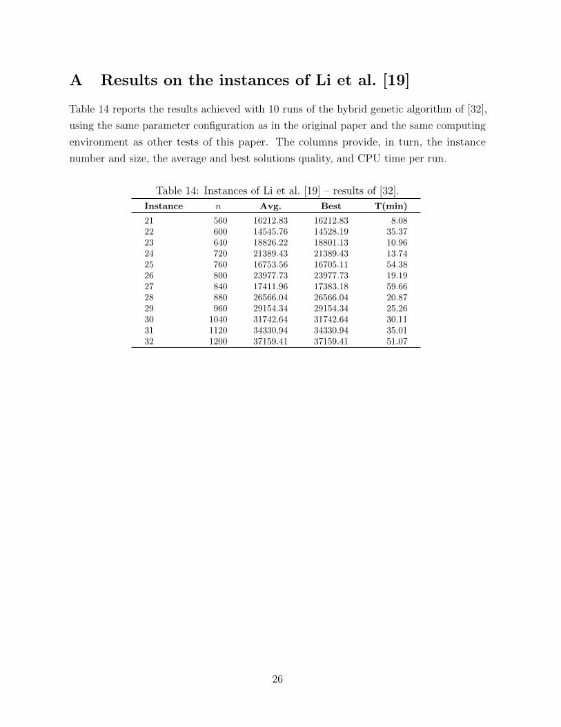
A Results on the instances of Li et al. [19]
Table 14 reports the results achieved with 10 runs of the hybrid genetic algorithm of [32],
using the same parameter configuration as in the original paper and the same computing
environment as other tests of this paper. The columns provide, in turn, the instance
number and size, the average and best solutions quality, and CPU time per run.
Table 14: Instances of Li et al. [19] – results of [32].
Instance n Avg. Best T(min)
21 560 16212.83 16212.83 8.0822 600 14545.76 14528.19 35.3723 640 18826.22 18801.13 10.9624 720 21389.43 21389.43 13.7425 760 16753.56 16705.11 54.3826 800 23977.73 23977.73 19.1927 840 17411.96 17383.18 59.6628 880 26566.04 26566.04 20.8729 960 29154.34 29154.34 25.2630 1040 31742.64 31742.64 30.1131 1120 34330.94 34330.94 35.0132 1200 37159.41 37159.41 51.07
26