Embed Size (px)
Citation preview
A Multivariate Threshold GARCH Model with
Time-varying Correlations
C.K. Kwan ∗ W.K. Li† K. Ng‡
Abstract
In this article, a Multivariate Threshold Generalized Autoregressive Conditional Het-
eroscedasticity model with time-varying correlation (VC-MTGARCH) is proposed. The
model extends the idea of Engle (2002) and Tse & Tsui (2002) in a threshold framework.
This model retains the interpretation of the univariate threshold GARCH model and al-
lows for dynamic conditional correlations. Extension of Bollerslev, Engle and Wooldridge
(1988) in a threshold framework is also proposed as a by-product. Techniques of model
identification, estimation and model checking are developed. Some simulation results are
reported on the finite sample distribution of the maximum likelihood estimate of the VC-
MTGARCH model. Real examples demonstrate the asymmetric behaviour of the mean
and the variance in financial time series and that the VC-MTGARCH model can capture
these phenomena.
∗Email: [email protected]. Department of Applied Mathematics, The Hong Kong Polytechnic Univer-
sity and Department of Statistics and Actuarial Science, The University of Hong Kong.†Email: [email protected]. Department of Statistics and Actuarial Science, The University of Hong Kong‡Email: [email protected] Department of Statistics and Actuarial Science, The University of Hong Kong
1
Keywords: VC-MTGARCH model; Varying correlation; Volatility
1 Introduction
During the last two decades, the modelling of conditional volatility in finance has been widely
discussed in the literature. As a model for financial data with a changing conditional variance,
Engle (1982) first proposed the autoregressive conditional heteroscedasticity (ARCH) model.
Bollerslev (1986) extended this into a generalized ARCH (GARCH) model. Engle & Gonzalez-
Rivera (1991) further extended the GARCH model to a semiparametric GARCH model which
does not assume a parametric form of the noise distribution. A tremendous literature now exists
for the GARCH model, for instance Li, Ling & McAleer (2002).
Incidentally, there have been growing interests in the nonlinear time series, for instance, the
self-exciting threshold autoregressive (SETAR) model of Tong (1978, 1980, 1983) and Tong &
Lim (1980). Various tests for nonlinearity have since been developed. Keenan (1985) constructed
a test for linearity which is an analogue of Tukey’s one degree of freedom for nonadditivity test.
Petruccelli (1986) proposed a portmanteau test for self-exciting threshold autoregressive non-
linearity model. Moreover, Tsay (1989) proposed an efficient procedure for testing threshold
nonlinearity and successfully illustrated its use via the analysis of high-frequency financial data.
During the time, many researchers have also extended the ARCH model to a nonlinear ARCH
model, for example Li & Lam (1995). Li & Li (1996) extended the threshold ARCH model to
a double-threshold ARCH model, which can handle the situation where both the conditional
mean and the conditional variance specifications are piecewise linear given previous informa-
tion. Brooks (2001) further extended the double-threshold ARCH model to a double-threshold
2
GARCH model.
After the development in univariate ARCH model, the study of multivariate ARCH models
becomes the next important issue. Bollerslev, Engle and Wooldridge (1988) suggested a basic
structure for a multivariate GARCH (MGARCH) model. Engle & Kroner (1995) proposed a
BEKK model which is a class of MGARCH model. Numerous applications of the multivariate
GARCH models have been applied to financial data. For instance, Bollerslev (1990) studied
the time-varying variance structure of the exchange rate in the European Monetary System.
Kroner & Claessens (1991) applied the models to evaluate the optimal debt portfolio in multi-
ple currencies. Thereafter, Tsay (1998) proposed a procedure for testing multivariate threshold
nonlinearity models and successfully illustrated its use via the analysis of monthly U.S. interest
rates and two daily river flow series of Iceland. In order to satisfy the necessary conditions pre-
sented by Engle, Granger and Kraft (1984) for the conditional-variance matrix of an estimated
MGARCH model to be positive definite, Bollerslev (1990) suggested a parsimonious constant-
correlation MGARCH model. The necessary conditions for positive definiteness can be easily
imposed during the optimization of the log-likelihood function. Engle & Susmel (1993) inves-
tigate some international stock markets that have similar time-varying volatility. The recent
work of Tse & Tsui (2002), Engle (2002) and that of Pelletier (2003) describe a parsimonious
MGARCH model that allows a time-varying correlation instead of a constant-correlation for-
mulation for the conditional variance equation. It is found that the time-varying model could
provide interesting and more realistic empirical results.
In this paper, a multivariate threshold GARCH (MTGARCH) model with time-varying
correlation (VC-MTGARCH) is proposed. The proposed model is an extension of the threshold
approach for nonlinearity to the time-varying correlation model of Tse & Tsui (2002). In
3
Section 2, the construction of a time-varying correlation MTGARCH model is discussed. A
nonlinearity test for model building is presented in section 3. Model identification and estimation
procedures of the proposed model are given in Section 4 and Section 5. Here, model identification
includes estimating the AR orders, GARCH orders, delay parameter and threshold parameter.
Simulation results are provided in Section 6. In Section 7, some empirical examples of the
proposed model using some real data sets are presented. These are the exchange rate data and
national stock market price data considered in Tse & Tsui (2002). Finally some concluding
remarks are given in the last section.
2 A time-varying correlation MTGARCH Model
In this section, time-varying correlation Multivariate Threshold GARCH models are presented.
Consider an n-dimensional multivariate time series Zt = (Z1t, . . . , Znt), where t = 1, . . . , T . The
conditional variance matrix of Zt follows a time-varying structure,
V ar(Zt|Ft−1) = Ht,
where Ft−1 is the information set {Zt−1, . . . , Z1} at time t − 1. Rewrite Ht = H12t H
12t , where
H12t is the symmetric square-root matrix based on the spectral decomposition. Let et = H
12t εt,
where εt ∼ N(0, I). Here, εt=(ε1t, . . . , εnt)′ is assumed to be independently distributed and
et = (e1t, . . . , ent)′ is conditionally normally distributed with mean zero and variance-covariance
matrix Ht. Here, v′ denotes the transpose of v.
In this article, a time-varying correlations MGARCH model with threshold structure (VC-
MTGARCH) is mainly discussed. Pelletier (2003) introduced a regime switching model of
constant correlations within each regime. In this work, an extension of the VC-MGARCH
4
model of Tse & Tsui (2002) using the threshold approach is discussed. This model will have
an appealing property of dynamic correlations within a regime. In particular, the time varying
conditional variance matrix Ht is defined as follows:
Ht = DtΓtDt.
Denote the variance elements of Ht by σ2it, for i = 1, . . . , n, and the covariance elements by σ2
ijt,
where 1 ≤ i < j ≤ n. Define Dt as a n × n diagonal matrix where the ith diagonal element is
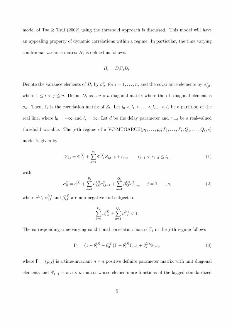
σit. Then, Γt is the correlation matrix of Zt. Let l0 < l1 < . . . < ls−1 < ls be a partition of the
real line, where l0 = −∞ and ls = ∞. Let d be the delay parameter and rt−d be a real-valued
threshold variable. The j-th regime of a VC-MTGARCH(p1, . . . , ps; P1, . . . , Ps; Q1, . . . , Qs; s)
model is given by
Zi,t = Φ(j)i,0 +
pj∑
k=1
Φ(j)i,kZi,t−k + ei,t, lj−1 < rt−d ≤ lj , (1)
with
σ2it = c
(j)i +
Pj∑
k=1
α(j)i,kσ2
i,t−k +Qj∑
k=1
β(j)i,k e2
i,t−k, j = 1, . . . , s, (2)
where c(j), α(j)i,k and β
(j)i,k are non-negative and subject to
Pj∑
k=1
α(j)i,k +
Qj∑
k=1
β(j)i,k < 1.
The corresponding time-varying conditional correlation matrix Γt in the j-th regime follows
Γt = (1 − θ(j)1 − θ
(j)2 )Γ + θ
(j)1 Γt−1 + θ
(j)2 Ψt−1, (3)
where Γ = {ρij} is a time-invariant n× n positive definite parameter matrix with unit diagonal
elements and Ψt−1 is a n × n matrix whose elements are functions of the lagged standardized
5
residuals ui,t =ei,t
σi,t
. The parameters θ(j)1 and θ
(j)2 are non-negative subject to θ
(j)1 + θ
(j)2 ≤ 1.
Denote Ψt = {Ψij,t}. In Tse & Tsui (2002), the matrix Ψt−1 follows
Ψij,t−1 =
M∑
h=1
ui,t−huj,t−h
√
√
√
√(M∑
h=1
u2i,t−h)(
M∑
h=1
u2j,t−h)
, (4)
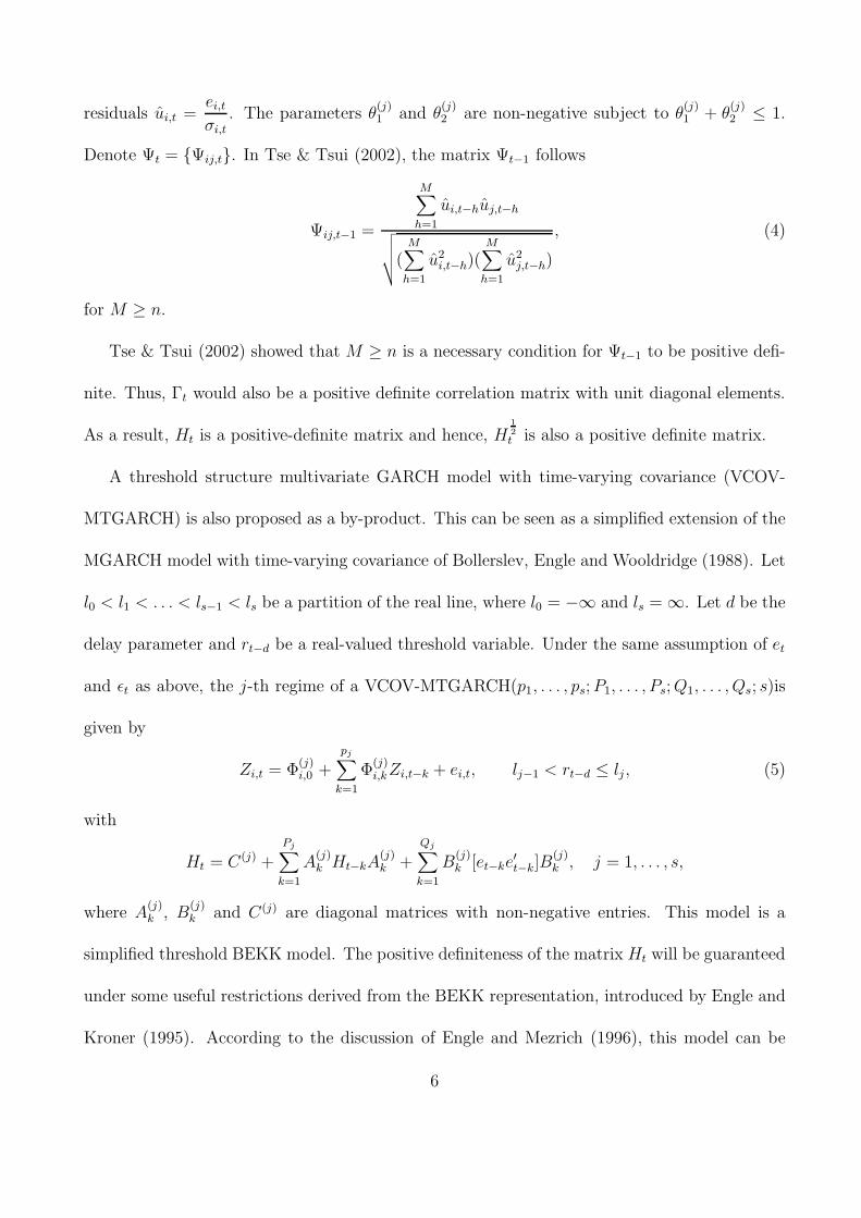
for M ≥ n.
Tse & Tsui (2002) showed that M ≥ n is a necessary condition for Ψt−1 to be positive defi-
nite. Thus, Γt would also be a positive definite correlation matrix with unit diagonal elements.
As a result, Ht is a positive-definite matrix and hence, H12t is also a positive definite matrix.
A threshold structure multivariate GARCH model with time-varying covariance (VCOV-
MTGARCH) is also proposed as a by-product. This can be seen as a simplified extension of the
MGARCH model with time-varying covariance of Bollerslev, Engle and Wooldridge (1988). Let
l0 < l1 < . . . < ls−1 < ls be a partition of the real line, where l0 = −∞ and ls = ∞. Let d be the
delay parameter and rt−d be a real-valued threshold variable. Under the same assumption of et
and εt as above, the j-th regime of a VCOV-MTGARCH(p1, . . . , ps; P1, . . . , Ps; Q1, . . . , Qs; s)is
given by
Zi,t = Φ(j)i,0 +
pj∑
k=1
Φ(j)i,kZi,t−k + ei,t, lj−1 < rt−d ≤ lj , (5)
with
Ht = C(j) +Pj∑
k=1
A(j)k Ht−kA
(j)k +
Qj∑
k=1
B(j)k [et−ke
′
t−k]B(j)k , j = 1, . . . , s,
where A(j)k , B
(j)k and C(j) are diagonal matrices with non-negative entries. This model is a
simplified threshold BEKK model. The positive definiteness of the matrix Ht will be guaranteed
under some useful restrictions derived from the BEKK representation, introduced by Engle and
Kroner (1995). According to the discussion of Engle and Mezrich (1996), this model can be
6
estimated subject to the variance targeting constraint by which the long run variance covariance
matrix is the sample covariance matrix.
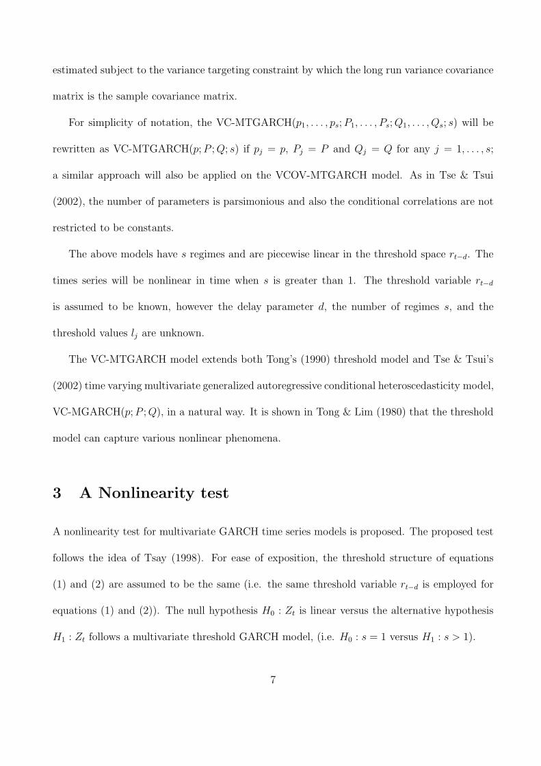
For simplicity of notation, the VC-MTGARCH(p1, . . . , ps; P1, . . . , Ps; Q1, . . . , Qs; s) will be
rewritten as VC-MTGARCH(p; P ; Q; s) if pj = p, Pj = P and Qj = Q for any j = 1, . . . , s;
a similar approach will also be applied on the VCOV-MTGARCH model. As in Tse & Tsui
(2002), the number of parameters is parsimonious and also the conditional correlations are not
restricted to be constants.
The above models have s regimes and are piecewise linear in the threshold space rt−d. The
times series will be nonlinear in time when s is greater than 1. The threshold variable rt−d
is assumed to be known, however the delay parameter d, the number of regimes s, and the
threshold values lj are unknown.
The VC-MTGARCH model extends both Tong’s (1990) threshold model and Tse & Tsui’s
(2002) time varying multivariate generalized autoregressive conditional heteroscedasticity model,
VC-MGARCH(p; P ; Q), in a natural way. It is shown in Tong & Lim (1980) that the threshold
model can capture various nonlinear phenomena.
3 A Nonlinearity test
A nonlinearity test for multivariate GARCH time series models is proposed. The proposed test
follows the idea of Tsay (1998). For ease of exposition, the threshold structure of equations
(1) and (2) are assumed to be the same (i.e. the same threshold variable rt−d is employed for
equations (1) and (2)). The null hypothesis H0 : Zt is linear versus the alternative hypothesis
H1 : Zt follows a multivariate threshold GARCH model, (i.e. H0 : s = 1 versus H1 : s > 1).
7
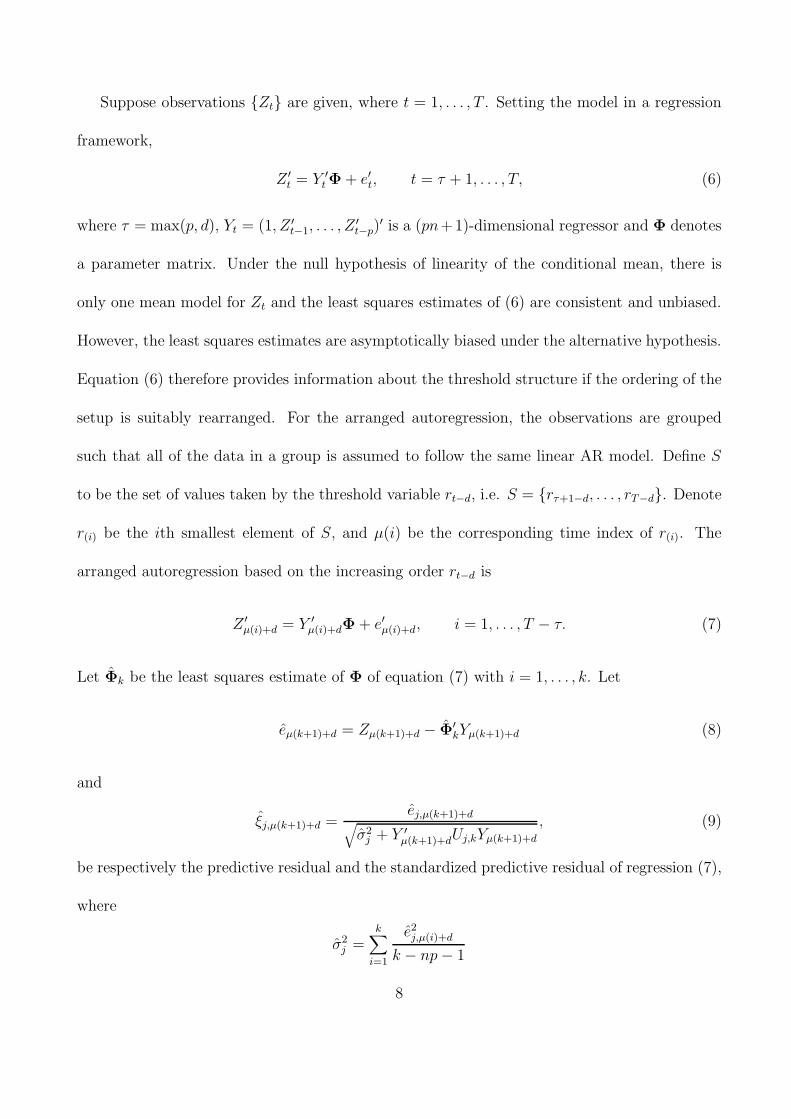
Suppose observations {Zt} are given, where t = 1, . . . , T . Setting the model in a regression
framework,
Z ′
t = Y ′
t Φ + e′t, t = τ + 1, . . . , T, (6)
where τ = max(p, d), Yt = (1, Z ′
t−1, . . . , Z′
t−p)′ is a (pn+1)-dimensional regressor and Φ denotes
a parameter matrix. Under the null hypothesis of linearity of the conditional mean, there is
only one mean model for Zt and the least squares estimates of (6) are consistent and unbiased.
However, the least squares estimates are asymptotically biased under the alternative hypothesis.
Equation (6) therefore provides information about the threshold structure if the ordering of the
setup is suitably rearranged. For the arranged autoregression, the observations are grouped
such that all of the data in a group is assumed to follow the same linear AR model. Define S
to be the set of values taken by the threshold variable rt−d, i.e. S = {rτ+1−d, . . . , rT−d}. Denote
r(i) be the ith smallest element of S, and µ(i) be the corresponding time index of r(i). The
arranged autoregression based on the increasing order rt−d is
Z ′
µ(i)+d = Y ′
µ(i)+dΦ + e′µ(i)+d, i = 1, . . . , T − τ. (7)
Let Φk be the least squares estimate of Φ of equation (7) with i = 1, . . . , k. Let
eµ(k+1)+d = Zµ(k+1)+d − Φ′
kYµ(k+1)+d (8)
and
ξj,µ(k+1)+d =ej,µ(k+1)+d
√
σ2j + Y ′
µ(k+1)+dUj,kYµ(k+1)+d
, (9)
be respectively the predictive residual and the standardized predictive residual of regression (7),
where
σ2j =
k∑
i=1
e2j,µ(i)+d
k − np − 1
8
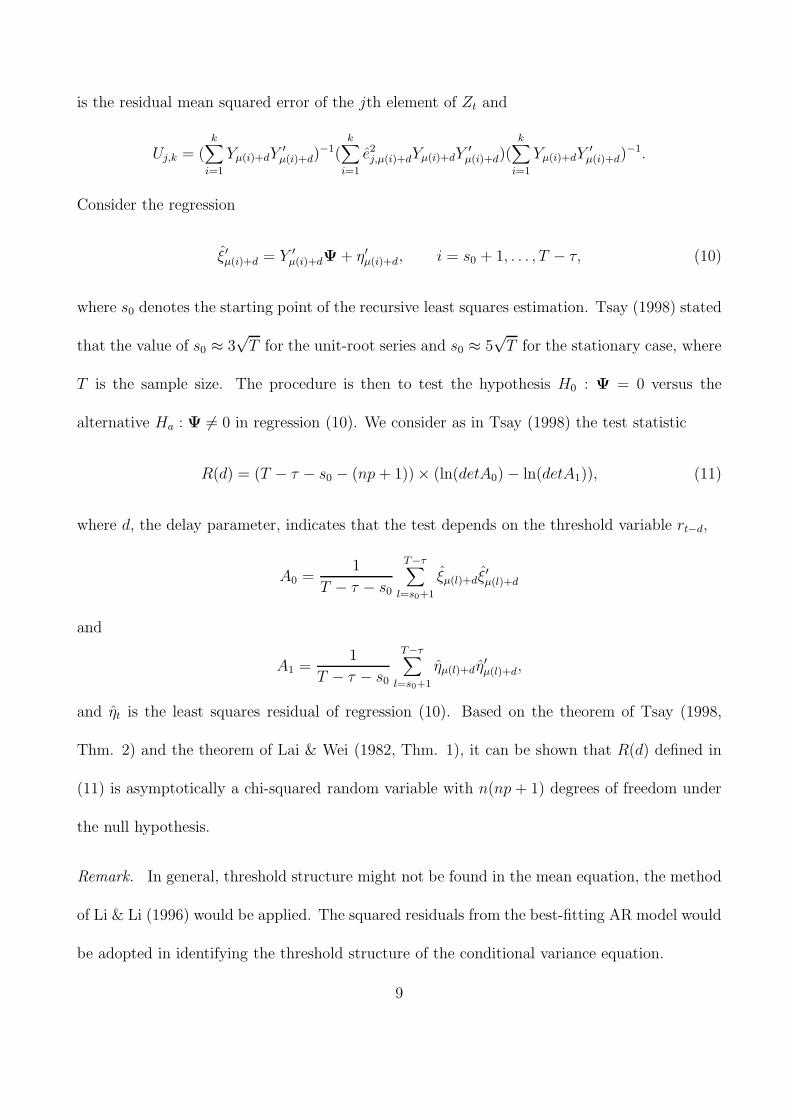
is the residual mean squared error of the jth element of Zt and
Uj,k = (k
∑
i=1
Yµ(i)+dY′
µ(i)+d)−1(
k∑
i=1
e2j,µ(i)+dYµ(i)+dY
′
µ(i)+d)(k
∑
i=1
Yµ(i)+dY′
µ(i)+d)−1.
Consider the regression
ξ′µ(i)+d = Y ′
µ(i)+dΨ + η′
µ(i)+d, i = s0 + 1, . . . , T − τ, (10)
where s0 denotes the starting point of the recursive least squares estimation. Tsay (1998) stated
that the value of s0 ≈ 3√
T for the unit-root series and s0 ≈ 5√
T for the stationary case, where
T is the sample size. The procedure is then to test the hypothesis H0 : Ψ = 0 versus the
alternative Ha : Ψ 6= 0 in regression (10). We consider as in Tsay (1998) the test statistic
R(d) = (T − τ − s0 − (np + 1)) × (ln(detA0) − ln(detA1)), (11)
where d, the delay parameter, indicates that the test depends on the threshold variable rt−d,
A0 =1
T − τ − s0
T−τ∑
l=s0+1
ξµ(l)+dξ′
µ(l)+d
and
A1 =1
T − τ − s0
T−τ∑
l=s0+1
ηµ(l)+dη′
µ(l)+d,
and ηt is the least squares residual of regression (10). Based on the theorem of Tsay (1998,
Thm. 2) and the theorem of Lai & Wei (1982, Thm. 1), it can be shown that R(d) defined in
(11) is asymptotically a chi-squared random variable with n(np + 1) degrees of freedom under
the null hypothesis.
Remark. In general, threshold structure might not be found in the mean equation, the method
of Li & Li (1996) would be applied. The squared residuals from the best-fitting AR model would
be adopted in identifying the threshold structure of the conditional variance equation.
9
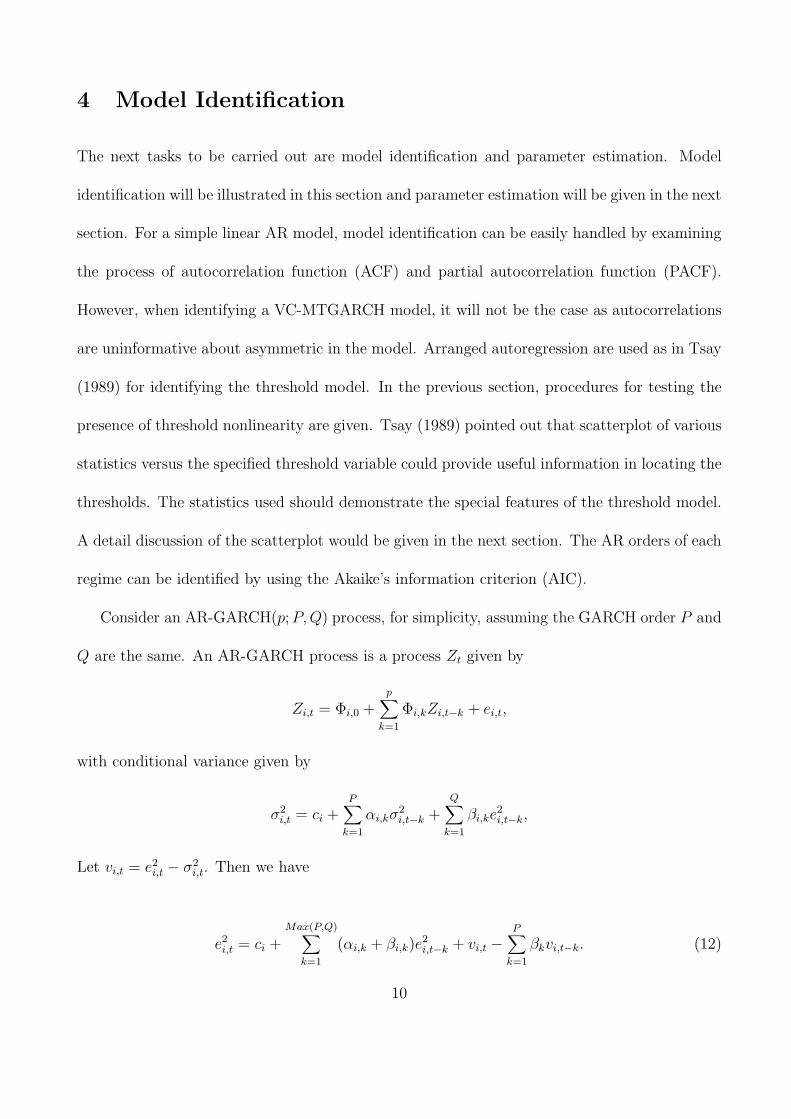
4 Model Identification
The next tasks to be carried out are model identification and parameter estimation. Model
identification will be illustrated in this section and parameter estimation will be given in the next
section. For a simple linear AR model, model identification can be easily handled by examining
the process of autocorrelation function (ACF) and partial autocorrelation function (PACF).
However, when identifying a VC-MTGARCH model, it will not be the case as autocorrelations
are uninformative about asymmetric in the model. Arranged autoregression are used as in Tsay
(1989) for identifying the threshold model. In the previous section, procedures for testing the
presence of threshold nonlinearity are given. Tsay (1989) pointed out that scatterplot of various
statistics versus the specified threshold variable could provide useful information in locating the
thresholds. The statistics used should demonstrate the special features of the threshold model.
A detail discussion of the scatterplot would be given in the next section. The AR orders of each
regime can be identified by using the Akaike’s information criterion (AIC).
Consider an AR-GARCH(p; P, Q) process, for simplicity, assuming the GARCH order P and
Q are the same. An AR-GARCH process is a process Zt given by
Zi,t = Φi,0 +p
∑
k=1
Φi,kZi,t−k + ei,t,
with conditional variance given by
σ2i,t = ci +
P∑
k=1
αi,kσ2i,t−k +
Q∑
k=1
βi,ke2i,t−k,
Let vi,t = e2i,t − σ2
i,t. Then we have
e2i,t = ci +
Max(P,Q)∑
k=1
(αi,k + βi,k)e2i,t−k + vi,t −
P∑
k=1
βkvi,t−k. (12)
10

Gourieroux (1997, p.37) shows that E(vi,t −P
∑
k=1
βkvi,t−k|Ft−1) = 0. Therefore, the MGARCH
model can be rewritten in an ARMA representation. This is useful in identifying the GARCH
orders P and Q.
The model identification procedure mainly involves two parts:
• Applying Tsay’s procedure to identify the delay parameters, the threshold parameters and
the AR orders in the conditional mean.
• Identify the GARCH orders of the conditional variances.
The overall procedure is as follows.
1. Select the AR order p, the GARCH order P, Q.
2. Fit arranged autoregressions for a given p and each possible delays d, and perform the
threshold nonlinearity test. When nonlinearity is detected, choose the delay parameter d
which maximizes the test statistics.
3. For given p and d, locate the value of the threshold parameter by using Tsay’ arranged
autoregression based on the scatterplots of the elements of Φ versus the threshold variable.
4. If the threshold structure is identified, calculate the residuals et of the threshold AR
model and identify the GARCH order using ete′
t and equation (12). Then fit the entire
VC-MTGARCH model.
5. Use an information criterion like AIC or Bayesian information criterion (BIC) to refine
the AR orders, the GARCH orders, the delay and threshold parameters by repeating steps
(1) - (4), if necessary.
11
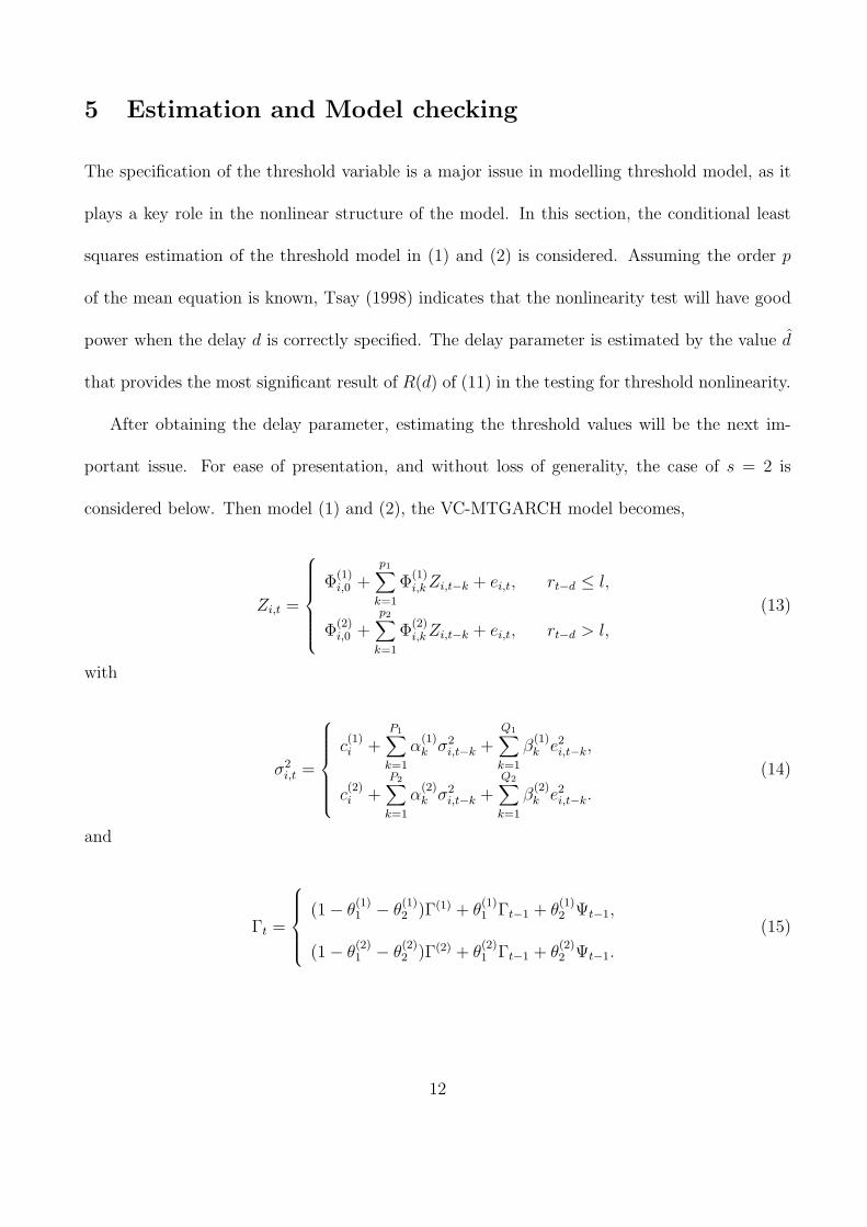
5 Estimation and Model checking
The specification of the threshold variable is a major issue in modelling threshold model, as it
plays a key role in the nonlinear structure of the model. In this section, the conditional least
squares estimation of the threshold model in (1) and (2) is considered. Assuming the order p
of the mean equation is known, Tsay (1998) indicates that the nonlinearity test will have good
power when the delay d is correctly specified. The delay parameter is estimated by the value d
that provides the most significant result of R(d) of (11) in the testing for threshold nonlinearity.
After obtaining the delay parameter, estimating the threshold values will be the next im-
portant issue. For ease of presentation, and without loss of generality, the case of s = 2 is
considered below. Then model (1) and (2), the VC-MTGARCH model becomes,
Zi,t =
Φ(1)i,0 +
p1∑
k=1
Φ(1)i,k Zi,t−k + ei,t, rt−d ≤ l,
Φ(2)i,0 +
p2∑
k=1
Φ(2)i,k Zi,t−k + ei,t, rt−d > l,
(13)
with
σ2i,t =
c(1)i +
P1∑
k=1
α(1)k σ2
i,t−k +Q1∑
k=1
β(1)k e2
i,t−k,
c(2)i +
P2∑
k=1
α(2)k σ2
i,t−k +Q2∑
k=1
β(2)k e2
i,t−k.
(14)
and
Γt =
(1 − θ(1)1 − θ
(1)2 )Γ(1) + θ
(1)1 Γt−1 + θ
(1)2 Ψt−1,
(1 − θ(2)1 − θ
(2)2 )Γ(2) + θ
(2)1 Γt−1 + θ
(2)2 Ψt−1.
(15)
12
Chan (1993) has shown the strong consistency of the estimator of a threshold model. In
particular, the threshold value is super-consistent in the sense that, l = l + Op(1/N). We now
propose a method for estimating the threshold values. For simplicity, the same threshold struc-
ture of the mean and conditional variance equations are considered. When there is a threshold
structure in the mean equation, it is noted in Section 3 that the least squares estimates of the
mean equation are biased. Then we can take this into account by the arranged autoregression
method.
The next step is to locate the threshold value l, so that we can divide observations into
regimes. To do this, the true value of l satisfies rµ(s) ≤ l < rµ(s+1). In general, there are several
methods to estimate the threshold values. Tsay (1989) considered the empirical percentiles as
candidates for the threshold values. In this articles, all the values in the set S are considered
to be candidates for the threshold values. We also adopt the approach of Tsay (1989) by
considering scatterplots of various statistics versus the specified threshold variable as method
for locating the threshold. In the arranged autoregression framework, the threshold model
consists of various model changing at each candidate threshold value. For simplicity, the AR
order of the mean equation is usually taken to be of low order, say p = 1. Therefore, the values
of the lag-1 AR coefficients are biased at the threshold values. A scatterplot of the lag-1 AR
coefficients versus the threshold variable thus may reveal the locations of the threshold values.
At each candidate threshold value, the lag-1 AR coefficients in the first and second regime,
Φ(1)1 and Φ
(2)1 can be calculated respectively. However, the lag-1 AR coefficients have n different
values in each regime. In order to obtain a relevant scatterplot, we therefore have to consider
a real value deterministic function which can differentiate between Φ(1)1 and Φ
(2)1 . Here, the
deterministic function will be defined as the mean of all the entries of the lag-1 AR coefficients.
13
A scatterplot can then be obtained by plotting the values of the suggested deterministic function
against the values of the threshold variable. Following Tsay’s (1989) approach, the threshold
can be obtained.
After locating the threshold value, the series in each regime of model (13) becomes linear.
Moreover, the threshold structure also applies to (14). The remaining task is to estimate the
parameters in (14). Assuming normality, et|Ft−1 ∼ N(0, Ht), and the conditional loglikelihood
at time t, Lt is given by
Lt = −1
2(n log 2π + log |Ht| + e′tH
−1t et)
= −1
2(n log 2π + log |Γt| + log σ2
i,t + e′tD−1t Γ−1
t D−1t et)
and thus the loglikelihood function, L =T
∑
t=1
Lt can be obtained.
Remark. Asymptotic normality of the estimated parameter θ can be established as in Chan
(1993). In actual estimation, numerical derivative will be applied in the conjugate gradient
method instead. It is because the size of the data series usually are large enough so that the
estimated results using numerical derivative are still appropriate. In addition, the number of
operations in estimation required for the numerical derivative is much less than that for the
theoretical derivative. However, the derivatives of L will be useful if the sample size is small
because more information about the gradient is often required for speedy convergence.
In checking the adequacy of the ARMA models with homogeneous conditional covariance
over time, residual autocorrelations has been widely applied. Li (1992) proposed the asymptotic
distribution of residual autocorrelations of a general threshold nonlinear time series model. Li &
Mak (1994) provided the asymptotic distribution of squared residual autocorrelations of a gen-
eral conditional heteroscedastic nonlinear time series model. Tse (2002) proposed an asymptotic
14
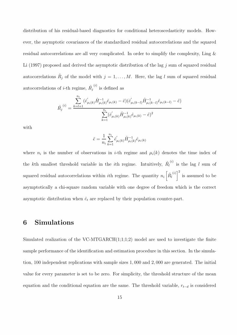
distribution of his residual-based diagnostics for conditional heteroscedasticity models. How-
ever, the asymptotic covariances of the standardized residual autocorrelations and the squared
residual autocorrelations are all very complicated. In order to simplify the complexity, Ling &
Li (1997) proposed and derived the asymptotic distribution of the lag j sum of squared residual
autocorrelations Rj of the model with j = 1, . . . , M . Here, the lag l sum of squared residual
autocorrelations of i-th regime, Rj
(i)is defined as
Rj
(i)=
ni∑
k=l+1
(e′
µi(k)H−1µi(k)eµi(k) − e)(e
′
µi(k−l)H−1µi(k−l)eµi(k−l) − e)
ni∑
k=1
(e′
µi(k)H−1µi(k)eµi(k) − e)2
with
e =1
ni
ni∑
k=1
e′
µi(k)H−1µi(k)eµi(k)
where ni is the number of observations in i-th regime and µi(k) denotes the time index of
the kth smallest threshold variable in the ith regime. Intuitively, Rl
(i)is the lag l sum of
squared residual autocorrelations within ith regime. The quantity ni
[
Rl
(i)]2
is assumed to be
asymptotically a chi-square random variable with one degree of freedom which is the correct
asymptotic distribution when et are replaced by their population counter-part.
6 Simulations
Simulated realization of the VC-MTGARCH(1;1;1;2) model are used to investigate the finite
sample performance of the identification and estimation procedure in this section. In the simula-
tion, 100 independent replications with sample sizes 1, 000 and 2, 000 are generated. The initial
value for every parameter is set to be zero. For simplicity, the threshold structure of the mean
equation and the conditional equation are the same. The threshold variable, rt−d is considered
15
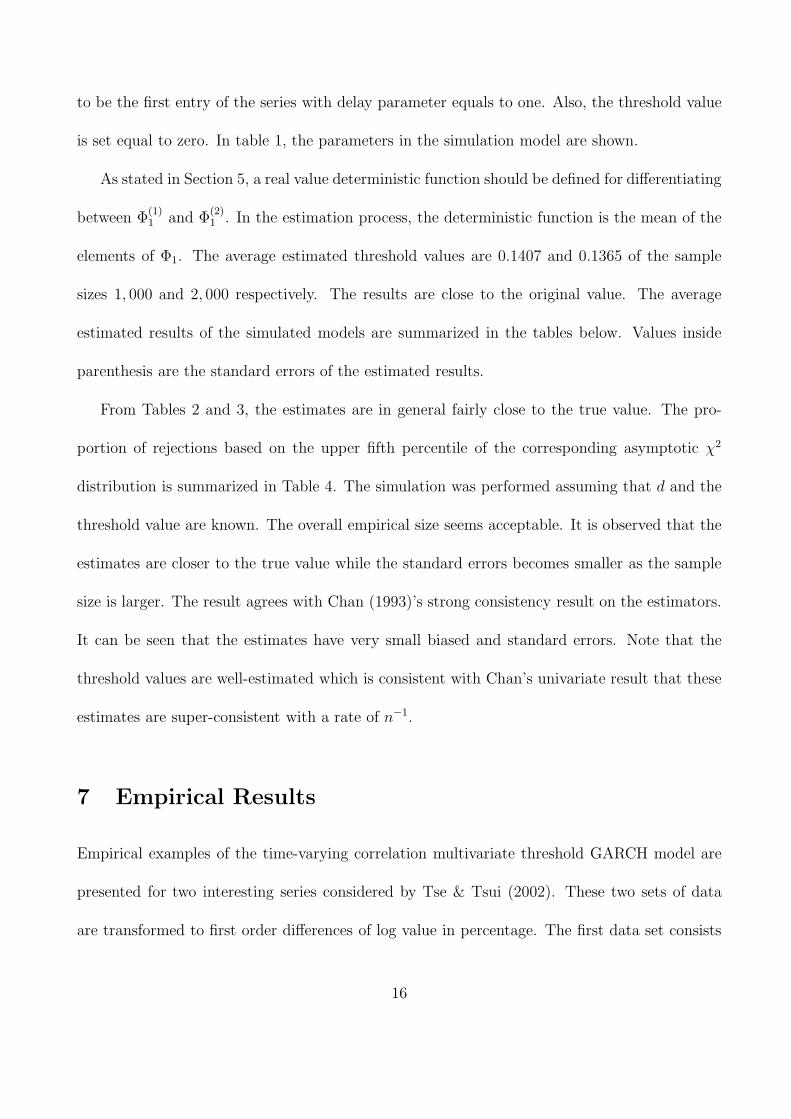
to be the first entry of the series with delay parameter equals to one. Also, the threshold value
is set equal to zero. In table 1, the parameters in the simulation model are shown.
As stated in Section 5, a real value deterministic function should be defined for differentiating
between Φ(1)1 and Φ
(2)1 . In the estimation process, the deterministic function is the mean of the
elements of Φ1. The average estimated threshold values are 0.1407 and 0.1365 of the sample
sizes 1, 000 and 2, 000 respectively. The results are close to the original value. The average
estimated results of the simulated models are summarized in the tables below. Values inside
parenthesis are the standard errors of the estimated results.
From Tables 2 and 3, the estimates are in general fairly close to the true value. The pro-
portion of rejections based on the upper fifth percentile of the corresponding asymptotic χ2
distribution is summarized in Table 4. The simulation was performed assuming that d and the
threshold value are known. The overall empirical size seems acceptable. It is observed that the
estimates are closer to the true value while the standard errors becomes smaller as the sample
size is larger. The result agrees with Chan (1993)’s strong consistency result on the estimators.
It can be seen that the estimates have very small biased and standard errors. Note that the
threshold values are well-estimated which is consistent with Chan’s univariate result that these
estimates are super-consistent with a rate of n−1.
7 Empirical Results
Empirical examples of the time-varying correlation multivariate threshold GARCH model are
presented for two interesting series considered by Tse & Tsui (2002). These two sets of data
are transformed to first order differences of log value in percentage. The first data set consists
16
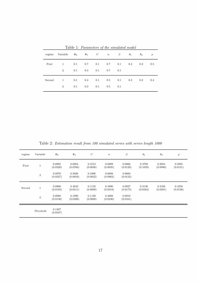
Table 1: Parameters of the simulated model
regime Variable Φ0 Φ1 C α β θ1 θ2 ρ
First 1 0.1 0.7 0.1 0.7 0.1 0.4 0.2 0.5
2 0.1 0.4 0.1 0.7 0.1
Second 1 0.1 0.4 0.1 0.5 0.1 0.3 0.2 0.4
2 0.1 0.2 0.1 0.5 0.1
Table 2: Estimation result from 100 simulated series with series length 1000
regime Variable Φ0 Φ1 C α β θ1 θ2 ρ
First 10.0905
(0.0320)0.6804
(0.0766)0.1012
(0.0036)0.6809
(0.0035)0.0866
(0.0120)0.3708
(0.1059)0.2024
(0.0090)0.5085
(0.0131)
20.0970
(0.0227)0.3926
(0.0656)0.1006
(0.0022)0.6808
(0.0962)0.0860
(0.0123)
Second 10.0960
(0.0193)0.4042
(0.0511)0.1132
(0.0098)0.4990
(0.0318)0.0927
(0.0173)0.3130
(0.0504)0.2168
(0.0291)0.4258
(0.0136)
20.0988
(0.0136)0.1990
(0.0396)0.1139
(0.0090)0.4908
(0.0230)0.0918
(0.0161)
Threshold0.1407
(0.0347)
17
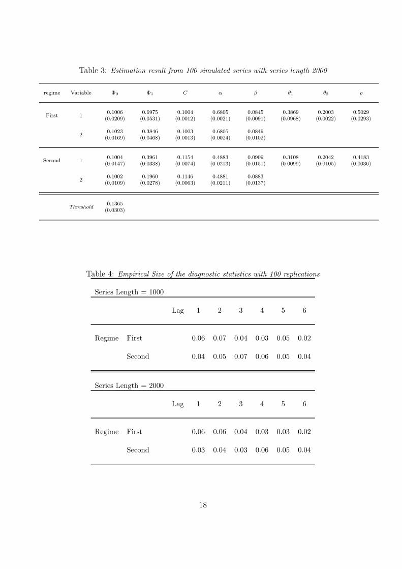
Table 3: Estimation result from 100 simulated series with series length 2000
regime Variable Φ0 Φ1 C α β θ1 θ2 ρ
First 10.1006
(0.0209)0.6975
(0.0531)0.1004
(0.0012)0.6805
(0.0021)0.0845
(0.0091)0.3869
(0.0968)0.2003
(0.0022)0.5029
(0.0293)
20.1023
(0.0169)0.3846
(0.0468)0.1003
(0.0013)0.6805
(0.0024)0.0849
(0.0102)
Second 10.1004
(0.0147)0.3961
(0.0338)0.1154
(0.0074)0.4883
(0.0213)0.0909
(0.0151)0.3108
(0.0099)0.2042
(0.0105)0.4183
(0.0036)
20.1002
(0.0109)0.1960
(0.0278)0.1146
(0.0063)0.4881
(0.0211)0.0883
(0.0137)
Threshold0.1365
(0.0303)
Table 4: Empirical Size of the diagnostic statistics with 100 replications
Series Length = 1000
Lag 1 2 3 4 5 6
Regime First 0.06 0.07 0.04 0.03 0.05 0.02
Second 0.04 0.05 0.07 0.06 0.05 0.04
Series Length = 2000
Lag 1 2 3 4 5 6
Regime First 0.06 0.06 0.04 0.03 0.03 0.02
Second 0.03 0.04 0.03 0.06 0.05 0.04
18
of the stock market indices of the Hong Kong and the Singapore markets, the Hang Seng Index
(HSI) and the Straits Time Index (SES) for Hong Kong and Singapore respectively. These
series represent 1,942 daily (closing) prices for each series from January 1990 through March
1998. The second data set consists of two exchange rate (versus U.S. dollar) series, namely the
Deutsche Mark and the Japanese Yen. There are 2,131 daily observations covering the period
from January 1990 through June 1998. Tse & Tsui (2002) suggested a parsimonious AR order
of the conditional mean equation to fit these two data sets. According to the model checking
discussed in Section 5, the lag-l sum of squared (standardized) residual autocorrelations are also
given below assuming M = 6 for each of the considered data set.
7.1 Hang Seng Index and Straits Time Index
The dramatic rise in the HSI over the latter 1990s puzzled many portfolio managers. Tse &
Tsui (2002) pointed out that the national stock markets in Hong Kong experienced different
phases of bulls and bears over the 1990s. It is also found that the HSI has always been more
volatile than the SES but that this gap widens at the end of this sample. Tse & Tsui (2002)
showed that significant serial autocorrelations are present.
Here, the VC-MTGARCH(1;1;1;2) model is used to fit this data set. Let Z1,t represents the
HSI and Z2,t represents the SES. Graphically, it suggests that the stock market indices in Hong
Kong have a larger volatility than Singapore. During the observed period, it is known that the
HSI has a giant rise before 1997, while there is a huge drop in 1998. It is believed that there
may be a structural change in the economy and hence a threshold model would be relevant. Let
the lagged values (d = 1) of the HSI, Z1,t−1 be the threshold variable. The nonlinearity test
statistic, R(d) = 80.13. The asymptotic distribution of the statistics is χ2 with 6 df. Therefore
19
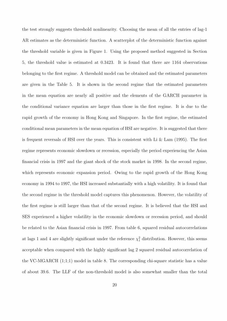
the test strongly suggests threshold nonlinearity. Choosing the mean of all the entries of lag-1
AR estimates as the deterministic function. A scatterplot of the deterministic function against
the threshold variable is given in Figure 1. Using the proposed method suggested in Section
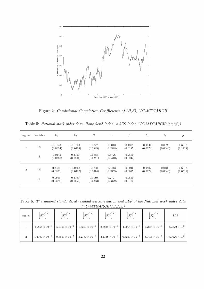
5, the threshold value is estimated at 0.3423. It is found that there are 1164 observations
belonging to the first regime. A threshold model can be obtained and the estimated parameters
are given in the Table 5. It is shown in the second regime that the estimated parameters
in the mean equation are nearly all positive and the elements of the GARCH parameter in
the conditional variance equation are larger than those in the first regime. It is due to the
rapid growth of the economy in Hong Kong and Singapore. In the first regime, the estimated
conditional mean parameters in the mean equation of HSI are negative. It is suggested that there
is frequent reversals of HSI over the years. This is consistent with Li & Lam (1995). The first
regime represents economic slowdown or recession, especially the period experiencing the Asian
financial crisis in 1997 and the giant shock of the stock market in 1998. In the second regime,
which represents economic expansion period. Owing to the rapid growth of the Hong Kong
economy in 1994 to 1997, the HSI increased substantially with a high volatility. It is found that
the second regime in the threshold model captures this phenomenon. However, the volatility of
the first regime is still larger than that of the second regime. It is believed that the HSI and
SES experienced a higher volatility in the economic slowdown or recession period, and should
be related to the Asian financial crisis in 1997. From table 6, squared residual autocorrelations
at lags 1 and 4 are slightly significant under the reference χ21 distribution. However, this seems
acceptable when compared with the highly significant lag 2 squared residual autocorrelation of
the VC-MGARCH (1;1;1) model in table 8. The corresponding chi-square statistic has a value
of about 39.6. The LLF of the non-threshold model is also somewhat smaller than the total
20
−3 −2 −1 0 1 2 3 4 5−0.8
−0.7
−0.6
−0.5
−0.4
−0.3
−0.2
−0.1
0
0.1
Threshold variable
Det
erm
inis
tic fu
nctio
n
Figure 1: Threshold value plot of National stock market data.
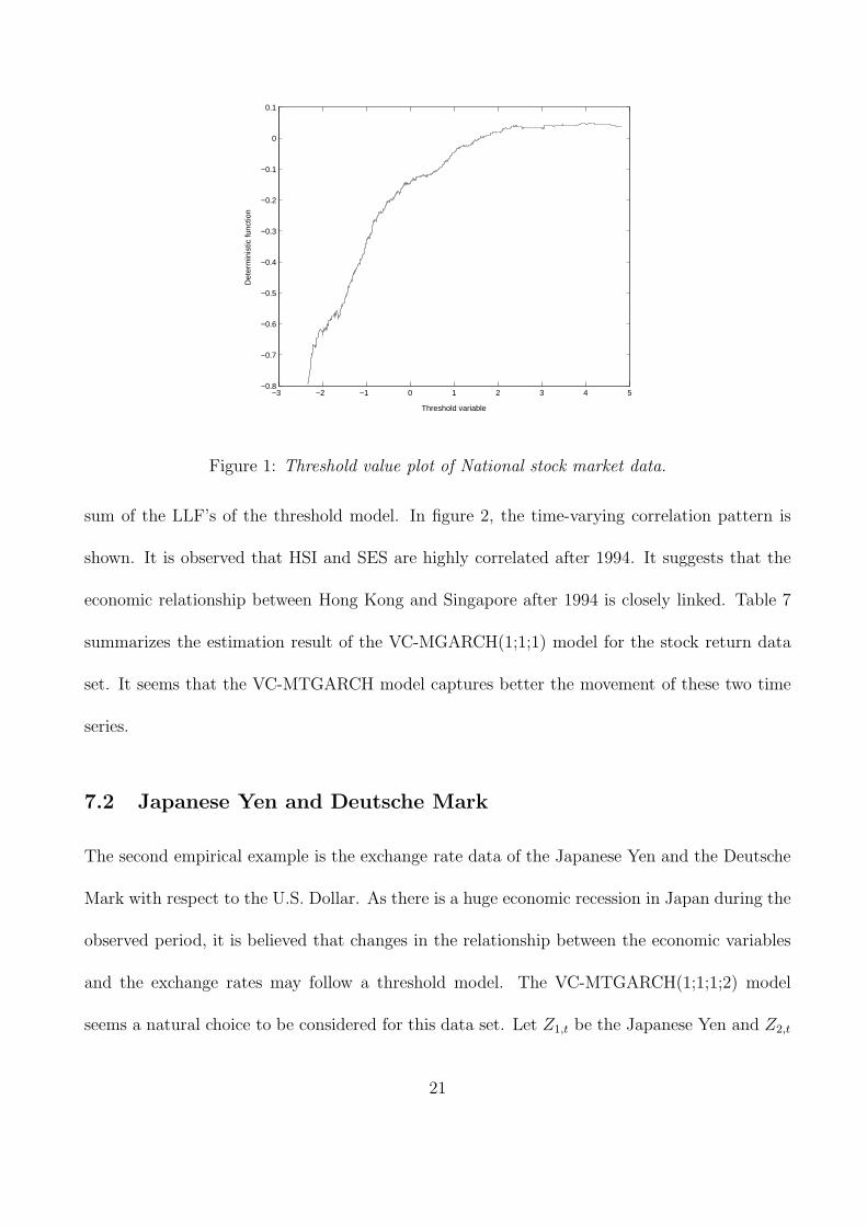
sum of the LLF’s of the threshold model. In figure 2, the time-varying correlation pattern is
shown. It is observed that HSI and SES are highly correlated after 1994. It suggests that the
economic relationship between Hong Kong and Singapore after 1994 is closely linked. Table 7
summarizes the estimation result of the VC-MGARCH(1;1;1) model for the stock return data
set. It seems that the VC-MTGARCH model captures better the movement of these two time
series.
7.2 Japanese Yen and Deutsche Mark
The second empirical example is the exchange rate data of the Japanese Yen and the Deutsche
Mark with respect to the U.S. Dollar. As there is a huge economic recession in Japan during the
observed period, it is believed that changes in the relationship between the economic variables
and the exchange rates may follow a threshold model. The VC-MTGARCH(1;1;1;2) model
seems a natural choice to be considered for this data set. Let Z1,t be the Japanese Yen and Z2,t
21
0
0.1
0.2
0.3
0.4
0.5
0.6
0.7
Time: Jan 1990 to Mar 1998
Con
ditio
nal C
orre
latio
n C
oeffi
cien
ts
Figure 2: Conditional Correlation Coefficients of (H,S), VC-MTGARCH
Table 5: National stock index data, Hang Send Index vs SES Index (VC-MTGARCH(1;1;1;2))
regime Variable Φ0 Φ1 C α β θ1 θ2 ρ
1 H−0.1643(0.0634)
−0.1200(0.0409)
0.1827(0.0529)
0.8048(0.0328)
0.1808(0.0185)
0.9944(0.0073)
0.0026(0.0040)
0.6918(0.1428)
S−0.0442(0.0326)
0.1750(0.0301)
0.0868(0.0251)
0.6726(0.0410)
0.2570(0.0244)
2 H0.3181
(0.0820)−0.0368(0.0427)
0.1738(0.0614)
0.8443(0.0359)
0.0212(0.0095)
0.9802(0.0072)
0.0188(0.0043)
0.6018(0.0511)
S0.0605
(0.0376)0.1799
(0.0353)0.1189
(0.0263)0.7727
(0.0379)0.0850
(0.0170)
Table 6: The squared standardized residual autocorrelation and LLF of the National stock index data
(VC-MTGARCH(1;1;1;2))
regime
[
R(i)1
]2 [
R(i)2
]2 [
R(i)3
]2 [
R(i)4
]2 [
R(i)5
]2 [
R(i)6
]2
LLF
1 4.2855 × 10⁻³ 5.0103 × 10⁻⁴ 1.6301 × 10⁻⁴ 2.5835 × 10⁻⁴ 4.9904 × 10⁻³ 1.7854 × 10⁻³−4.7872 × 10³
2 1.4197 × 10⁻⁴ 9.7563 × 10⁻⁵ 3.2380 × 10⁻⁴ 3.4338 × 10⁻⁴ 6.5263 × 10⁻⁶ 8.9405 × 10⁻⁶−3.3026 × 10³
22
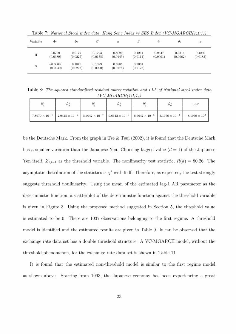
Table 7: National Stock index data, Hang Seng Index vs SES Index (VC-MGARCH(1;1;1))
Variable Φ0 Φ1 C α β θ1 θ2 ρ
H0.0709
(0.0389)0.0122
(0.0227)0.1793
(0.0175)0.8029
(0.0145)0.1241
(0.0111)0.9547
(0.0091)0.0314
(0.0062)0.4260
(0.0183)
S−0.0008(0.0240)
0.1876(0.0223)
0.1029(0.0090)
0.6985(0.0175)
0.2061(0.0176)
Table 8: The squared standardized residual autocorrelation and LLF of National stock index data
(VC-MGARCH(1;1;1))
R21 R2
2 R23 R2
4 R25 R2
6 LLF
7.8970 × 10⁻⁴ 2.0415 × 10⁻² 5.4042 × 10⁻⁷ 9.6642 × 10⁻⁶ 8.6647 × 10⁻⁵ 3.1976 × 10⁻⁴−8.1959 × 10³
be the Deutsche Mark. From the graph in Tse & Tsui (2002), it is found that the Deutsche Mark
has a smaller variation than the Japanese Yen. Choosing lagged value (d = 1) of the Japanese
Yen itself, Z1,t−1 as the threshold variable. The nonlinearity test statistic, R(d) = 80.26. The
asymptotic distribution of the statistics is χ2 with 6 df. Therefore, as expected, the test strongly
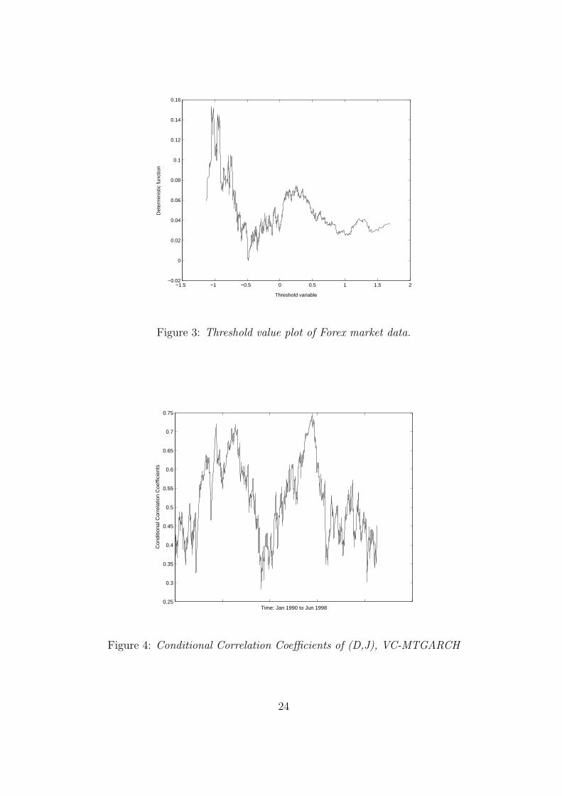
suggests threshold nonlinearity. Using the mean of the estimated lag-1 AR parameter as the
deterministic function, a scatterplot of the deterministic function against the threshold variable
is given in Figure 3. Using the proposed method suggested in Section 5, the threshold value
is estimated to be 0. There are 1037 observations belonging to the first regime. A threshold
model is identified and the estimated results are given in Table 9. It can be observed that the
exchange rate data set has a double threshold structure. A VC-MGARCH model, without the
threshold phenomenon, for the exchange rate data set is shown in Table 11.
It is found that the estimated non-threshold model is similar to the first regime model
as shown above. Starting from 1993, the Japanese economy has been experiencing a great
23
−1.5 −1 −0.5 0 0.5 1 1.5 2−0.02
0
0.02
0.04
0.06
0.08
0.1
0.12
0.14
0.16
Threshold variable
Det
erm
inis
tic fu
nctio
n
Figure 3: Threshold value plot of Forex market data.
0.25
0.3
0.35
0.4
0.45
0.5
0.55
0.6
0.65
0.7
0.75
Time: Jan 1990 to Jun 1998
Con
ditio
nal C
orre
latio
n C
oeffi
cien
ts
Figure 4: Conditional Correlation Coefficients of (D,J), VC-MTGARCH
24
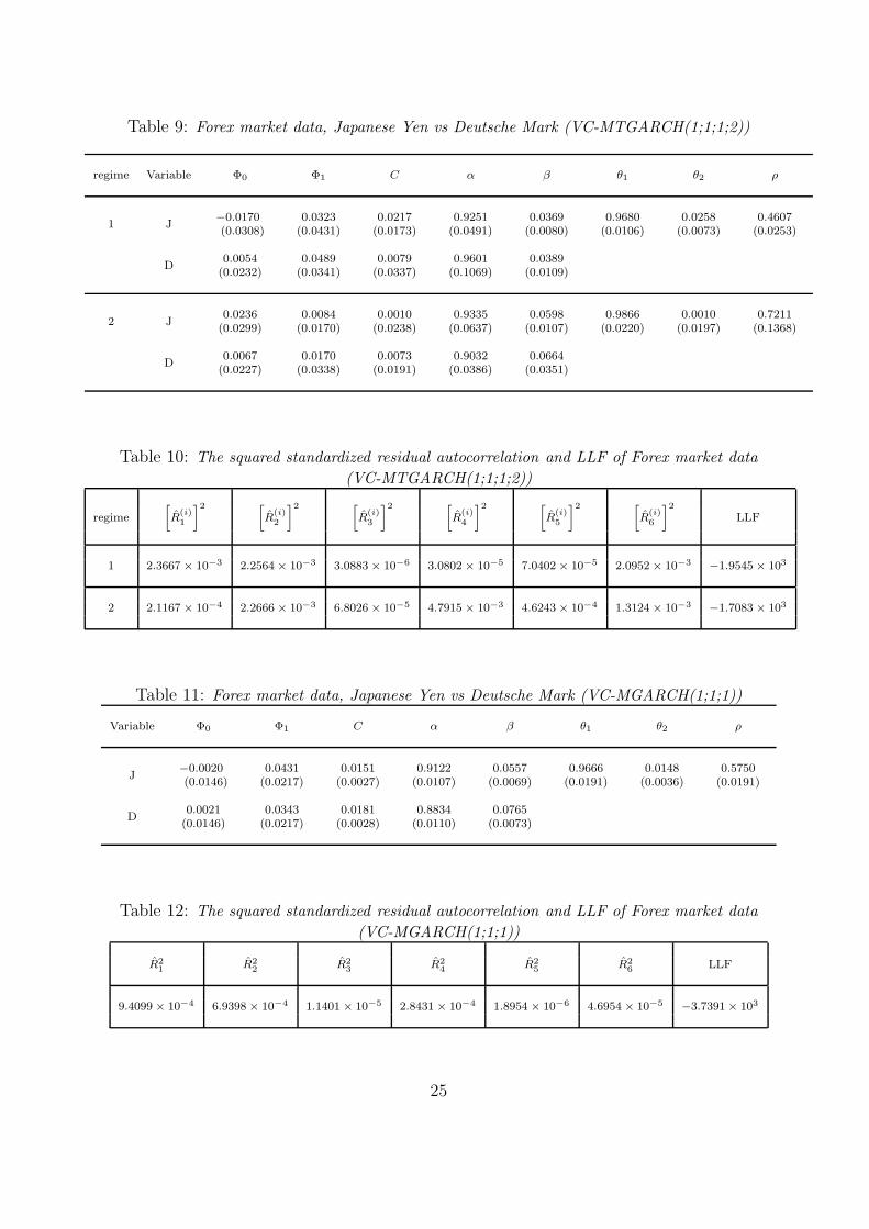
Table 9: Forex market data, Japanese Yen vs Deutsche Mark (VC-MTGARCH(1;1;1;2))
regime Variable Φ0 Φ1 C α β θ1 θ2 ρ
1 J−0.0170(0.0308)
0.0323(0.0431)
0.0217(0.0173)
0.9251(0.0491)
0.0369(0.0080)
0.9680(0.0106)
0.0258(0.0073)
0.4607(0.0253)
D0.0054
(0.0232)0.0489
(0.0341)0.0079
(0.0337)0.9601
(0.1069)0.0389
(0.0109)
2 J0.0236
(0.0299)0.0084
(0.0170)0.0010
(0.0238)0.9335
(0.0637)0.0598
(0.0107)0.9866
(0.0220)0.0010
(0.0197)0.7211
(0.1368)
D0.0067
(0.0227)0.0170
(0.0338)0.0073
(0.0191)0.9032
(0.0386)0.0664
(0.0351)
Table 10: The squared standardized residual autocorrelation and LLF of Forex market data
(VC-MTGARCH(1;1;1;2))
regime
[
R(i)1
]2 [
R(i)2
]2 [
R(i)3
]2 [
R(i)4
]2 [
R(i)5
]2 [
R(i)6
]2
LLF
1 2.3667 × 10⁻³ 2.2564 × 10⁻³ 3.0883 × 10⁻⁶ 3.0802 × 10⁻⁵ 7.0402 × 10⁻⁵ 2.0952 × 10⁻³−1.9545 × 10³
2 2.1167 × 10⁻⁴ 2.2666 × 10⁻³ 6.8026 × 10⁻⁵ 4.7915 × 10⁻³ 4.6243 × 10⁻⁴ 1.3124 × 10⁻³−1.7083 × 10³
Table 11: Forex market data, Japanese Yen vs Deutsche Mark (VC-MGARCH(1;1;1))
Variable Φ0 Φ1 C α β θ1 θ2 ρ
J−0.0020(0.0146)
0.0431(0.0217)
0.0151(0.0027)
0.9122(0.0107)
0.0557(0.0069)
0.9666(0.0191)
0.0148(0.0036)
0.5750(0.0191)
D0.0021
(0.0146)0.0343
(0.0217)0.0181
(0.0028)0.8834
(0.0110)0.0765
(0.0073)
Table 12: The squared standardized residual autocorrelation and LLF of Forex market data
(VC-MGARCH(1;1;1))
R21 R2
2 R23 R2
4 R25 R2
6 LLF
9.4099 × 10⁻⁴ 6.9398 × 10⁻⁴ 1.1401 × 10⁻⁵ 2.8431 × 10⁻⁴ 1.8954 × 10⁻⁶ 4.6954 × 10⁻⁵−3.7391 × 10³
25
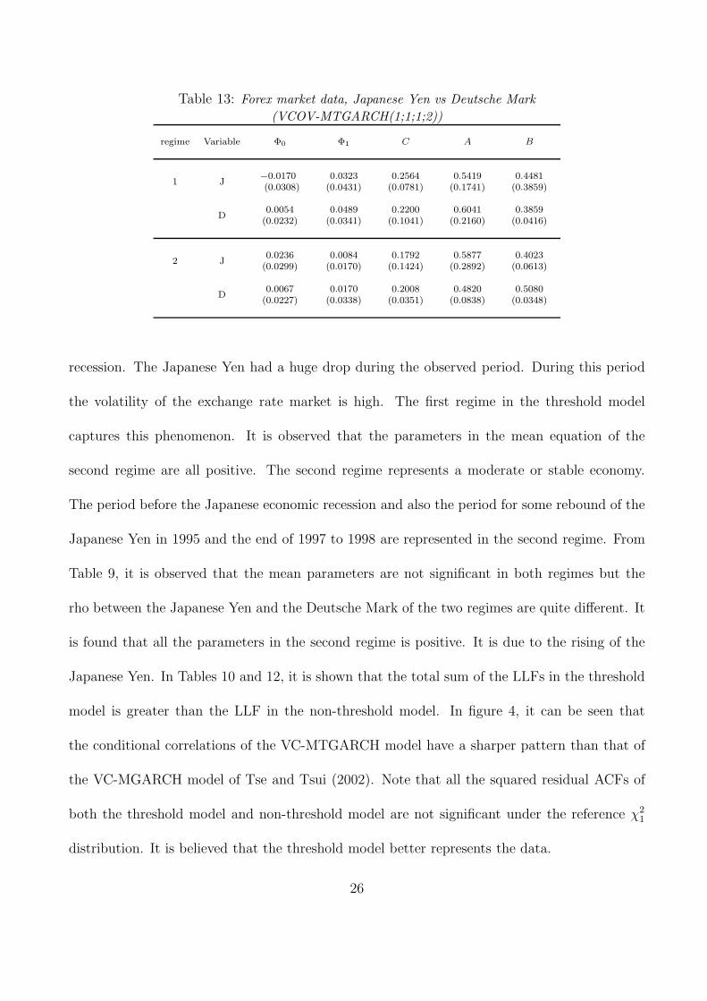
Table 13: Forex market data, Japanese Yen vs Deutsche Mark
(VCOV-MTGARCH(1;1;1;2))
regime Variable Φ0 Φ1 C A B
1 J−0.0170(0.0308)
0.0323(0.0431)
0.2564(0.0781)
0.5419(0.1741)
0.4481(0.3859)
D0.0054
(0.0232)0.0489
(0.0341)0.2200
(0.1041)0.6041
(0.2160)0.3859
(0.0416)
2 J0.0236
(0.0299)0.0084
(0.0170)0.1792
(0.1424)0.5877
(0.2892)0.4023
(0.0613)
D0.0067
(0.0227)0.0170
(0.0338)0.2008
(0.0351)0.4820
(0.0838)0.5080
(0.0348)
recession. The Japanese Yen had a huge drop during the observed period. During this period
the volatility of the exchange rate market is high. The first regime in the threshold model
captures this phenomenon. It is observed that the parameters in the mean equation of the
second regime are all positive. The second regime represents a moderate or stable economy.
The period before the Japanese economic recession and also the period for some rebound of the
Japanese Yen in 1995 and the end of 1997 to 1998 are represented in the second regime. From
Table 9, it is observed that the mean parameters are not significant in both regimes but the
rho between the Japanese Yen and the Deutsche Mark of the two regimes are quite different. It
is found that all the parameters in the second regime is positive. It is due to the rising of the
Japanese Yen. In Tables 10 and 12, it is shown that the total sum of the LLFs in the threshold
model is greater than the LLF in the non-threshold model. In figure 4, it can be seen that
the conditional correlations of the VC-MTGARCH model have a sharper pattern than that of
the VC-MGARCH model of Tse and Tsui (2002). Note that all the squared residual ACFs of
both the threshold model and non-threshold model are not significant under the reference χ21
distribution. It is believed that the threshold model better represents the data.
26
−0.8
−0.6
−0.4
−0.2
0
0.2
0.4
0.6
0.8
1
Time: Jan 1990 to Jun 1998
Con
ditio
nal C
orre
latio
n C
oeffi
cien
ts
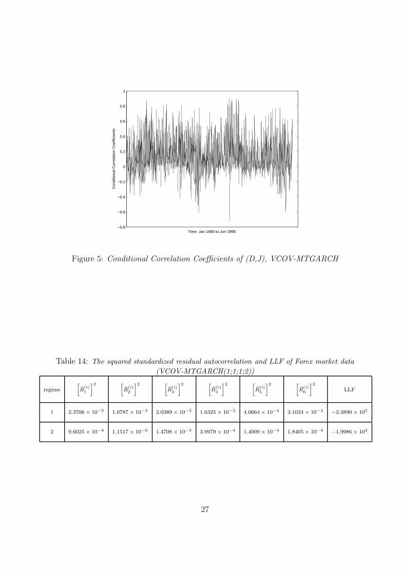
Figure 5: Conditional Correlation Coefficients of (D,J), VCOV-MTGARCH
Table 14: The squared standardized residual autocorrelation and LLF of Forex market data
(VCOV-MTGARCH(1;1;1;2))
regime
[
R(i)1
]2 [
R(i)2
]2 [
R(i)3
]2 [
R(i)4
]2 [
R(i)5
]2 [
R(i)6
]2
LLF
1 2.3706 × 10⁻³ 1.0787 × 10⁻³ 2.0389 × 10⁻³ 1.6325 × 10⁻³ 4.0664 × 10⁻⁴ 3.1034 × 10⁻⁴−2.3890 × 10³
2 9.6025 × 10⁻⁴ 1.1517 × 10⁻⁶ 1.4708 × 10⁻³ 3.9979 × 10⁻⁴ 1.4009 × 10⁻⁴ 1.8405 × 10⁻⁴−1.9986 × 10³
27
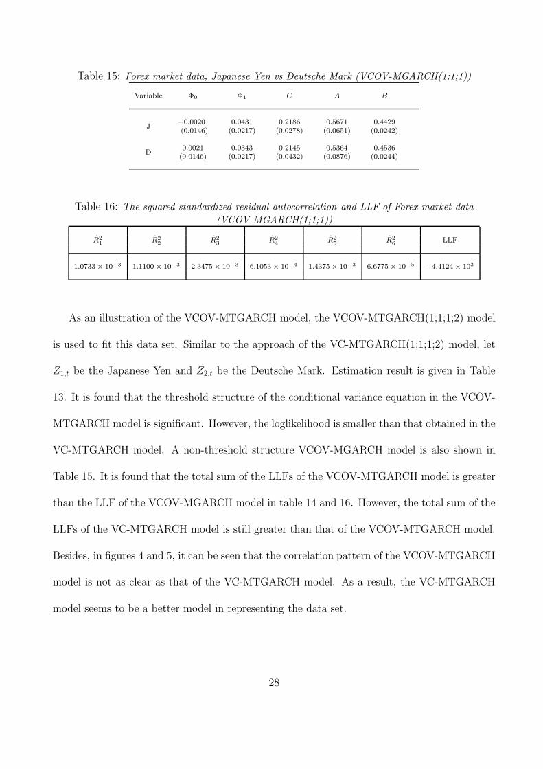
Table 15: Forex market data, Japanese Yen vs Deutsche Mark (VCOV-MGARCH(1;1;1))
Variable Φ0 Φ1 C A B
J−0.0020(0.0146)
0.0431(0.0217)
0.2186(0.0278)
0.5671(0.0651)
0.4429(0.0242)
D0.0021
(0.0146)0.0343
(0.0217)0.2145
(0.0432)0.5364
(0.0876)0.4536
(0.0244)
Table 16: The squared standardized residual autocorrelation and LLF of Forex market data
(VCOV-MGARCH(1;1;1))
R21 R2
2 R23 R2
4 R25 R2
6 LLF
1.0733 × 10⁻³ 1.1100 × 10⁻³ 2.3475 × 10⁻³ 6.1053 × 10⁻⁴ 1.4375 × 10⁻³ 6.6775 × 10⁻⁵−4.4124 × 10³
As an illustration of the VCOV-MTGARCH model, the VCOV-MTGARCH(1;1;1;2) model
is used to fit this data set. Similar to the approach of the VC-MTGARCH(1;1;1;2) model, let
Z1,t be the Japanese Yen and Z2,t be the Deutsche Mark. Estimation result is given in Table
13. It is found that the threshold structure of the conditional variance equation in the VCOV-
MTGARCH model is significant. However, the loglikelihood is smaller than that obtained in the
VC-MTGARCH model. A non-threshold structure VCOV-MGARCH model is also shown in
Table 15. It is found that the total sum of the LLFs of the VCOV-MTGARCH model is greater
than the LLF of the VCOV-MGARCH model in table 14 and 16. However, the total sum of the
LLFs of the VC-MTGARCH model is still greater than that of the VCOV-MTGARCH model.
Besides, in figures 4 and 5, it can be seen that the correlation pattern of the VCOV-MTGARCH
model is not as clear as that of the VC-MTGARCH model. As a result, the VC-MTGARCH
model seems to be a better model in representing the data set.
28
8 Conclusion
The model structure of the VC-MTGARCH is an extension and a synthesis of the work of Tong,
Tsay, Tse & Tsui (2002) and Engle (2002). The conditional variance matrix is easily guaranteed
to be positive definite and the conditional correlations are allowed to be non-constants. The
number of parameters of the model is also parsimonious. A modelling methodology is proposed
for the VC-MTGARCH model. Extensions of Tsay’s identification procedures are made to
identify the AR orders, GARCH orders, delay parameters and threshold parameters. Some
simulation results are presented. As a by-product of the VC-MTGARCH model, the multivariate
threshold GARCH model with time-varying covariance (VCOV-MTGARCH) is also defined. For
empirical applications, the VC-MTGARCH and VCOV-MTGARCH models are applied to the
data sets in Tse & Tsui (2002). The obtained VC-MTGARCH and VCOV-MTGARCH model
seem to capture well the threshold structure in the series. However, the correlation pattern
of the VC-MTGARCH model is more clear than that obtained by the VCOV-MTGARCH
model. Moreover, the loglikelihood of the VC-MTGARCH model is greater than that of the
VCOV-MTGARCH model. This suggests that the proposed VC-MTGARCH model should be
a potentially useful tool in modelling financial time series.
Acknowledgements — W.K. Li thanks the Hong Kong Research Grants Councils & the Croucher
Foundation for partial support of this research. We would also like to thank Professor Y.K. Tse
for providing the two financial time series data sets.
29
References
[1] Bollerslev, T. (1986), Generalized Autoregressive Conditional Heteroskedasticity, Journal
of Econometrics, 31, pp. 307 - 327.
[2] Bollerslev, T. (1990), Modelling the Coherence in Short-Run Nominal Exchange Rates: A
Multivariate Generalized ARCH Model, Review of Economics and Statistics, 72, pp. 498 -
505.
[3] Bollerslev, T., Engle, R.F. and Wooldridge, J.M. (1988), A Capital Asset Pricing Model
with Time-varying Covariances, Journal of Political Economy, 96, No. 1, pp. 116 - 131.
[4] Brooks, C. (2001), A double-threshold GARCH model for the French Franc/Deutschmark
exchange rate, Journal of Forecasting, 20, pp. 135 - 143.
[5] Chan, K.S. (1993), Consistency and Limiting Distribution of the Least Squares Estimator
of a Threshold Autoregressive Model, Annals of Statistics, 21, 1, pp. 520 - 533.
[6] Engle, R.F. (1982), Autoregressive Conditional Heteroscedasticity with Estimates of the
Variance of United Kingdom Inflation, Econometrica, 50, pp. 987 - 1007.
[7] Engle, R.F. (2002), Dynamic Conditional Correlation: A simple Class of Multivariate
Generalized Autoregressive Conditional Heteroskedasticity Models, Journal of Business
and Economic Statistics, 20, 3, pp. 339 - 350.
[8] Engle, R.F. and Gonzalez-Riveria, G. (1991), Semiparametric ARCH models, Journal of
Business and Economic Statistics, 9, 4, pp. 345 - 359.
30

[9] Engle, R.F. and Kroner, K.F. (1995), Multivariate Simultaneous Generalized ARCH,
Econometric Theory, 11, pp. 122 - 150.
[10] Engle, R.F. and Mezrich, J. (1996), GARCH for Groups, Risk, 9, pp. 36 - 40.
[11] Engle, R.F. and Susmel, R. (1993), Common Volatility in International Equity Market,
Journal of Business and Economic Statistics, 11, 2, pp. 167 - 176.
[12] Engle, R.F., Granger, C.W.J. and Kraft, D. (1984), Combining Competing Forecasts of
Inflation Using a Bivariate ARCH model, Journal of Economic Dynamics and Control, 8,
pp. 151 - 165.
[13] Gourieroux, C. (1997), ARCH Models and Financial Applications, Springer.
[14] Keenan, D.M. (1985), A Tukey nonadditivity-type test for time series nonlinearity,
Biometrika, 72, 1, pp. 39 - 44.
[15] Kroner, K.F. and Claessens, S. (1991), Optimal Dynamic Hedging Portfolios and the Cur-
rency Composition of External Debt, Journal of International Money and Finance, 10, pp.
131 - 148.
[16] Lai, T.L. and Wei, C.Z. (1982), Least Squares Estimates in Stochastic Regression Mod-
els with Applications to Identification and Control of Dynamic Systems, The Annals of
Statistics, 10, pp. 154 - 166.
[17] Li, C.W. and Li, W.K. (1996), On a Double-Threshold Autoregressive Heteroscedastic
Time Series Model, Journal in Applied Econometrics, Vol 11, pp. 253 - 274.
31
[18] Li, W.K. (1992), On the asymptotic standard errors of residual autocorrelations in nonlinear
Time Series Modelling, Biometrika, 79, 2, pp. 435 - 437.
[19] Li, W.K. and Lam, K. (1995), Modelling asymmetry in stock returns by a threshold ARCH
model, The Statistician, 44, 3, pp. 333 - 341.
[20] Li, W.K. and Mak, T.K. (1994), On the squared residual autocorrelations in conditional
heteroskedastic variance by iteratively weighted least squares, Journal of Time Series Anal-
ysis, 15, pp. 627 - 636.
[21] Li, W.K., Ling, S. and McAleer M. (2002), Recent theoretical results for time series models
with GARCH errors, Journal of Economic Surveys, 16, pp. 245 - 269.
[22] Ling, S.Q. and Li, W.K. (1997), Diagnostic checking of Nonlinear Multivariate Time Series
with Multivariate ARCH errors, Journal of Time Series Analysis, 18, pp. 447 - 464.
[23] MacRae, E.C. (1974), Matrix derivatives with an application to an adaptive linear decision
problem, The Annals of Statistics, 2, pp. 337 - 346.
[24] Pelletier, D. (2003), Regime switching for dynamic correlations, unpublished manuscript,
http://www4.ncsu.edu/∼dpellet.
[25] Petruccelli, J.D. and Davies, N. (1986), A portmanteau test for self-exciting threshold
autoregressive-type nonlinearity in time series, Biometrika, 73, 3, pp. 687 - 694.
[26] Tong, H. (1978), On a threshold model, (ed. C.H. Chen), Pattern Recognition and Signal
Processing, Sijthoff and Noordhoff, Amsterdam.
32
[27] Tong, H. (1980), A view on non-linear times series model building, Time series, (ed. O.D.
Anderson), North Holland, Amsterdam.
[28] Tong, H. (1983), Threshold models in non-linear time series analysis, Lecture Notes in
Statistics, No. 21. Springer, Heidelberg.
[29] Tong, H. (1990), Non-Linear Time Series: A Dynamical System Approach, Oxford Univer-
sity Press, Oxford.
[30] Tong, H. and K.S. Lim (1980), Threshold autoregressive, limit cycles and cyclical data,
Journal of the Royal Statistical Society, Series B, 42, pp. 245 - 292.
[31] Tsay, R.S. (1989), Testing and Modeling Threshold Autoregressive Processes, Journal of
the American Statistical Association, March 1989, 84, No. 405, pp. 231 - 240.
[32] Tsay, R.S. (1998), Testing and Modeling Multivariate Threshold Models, Journal of the
American Statistical Association, March 1998, 93, No. 443, pp. 1188 - 1202.
[33] Tse, Y.K. (2002), Residual-based diagnostics for conditional heteroscedasticity models,
Econometrics Journal, 5, pp. 358 - 373.
[34] Tse, Y.K. and Tsui, A.K.C. (2002), A Generalized Autoregressive Conditional Het-
eroscedasticity Model with Time-Varying Correlations, Journal of Business and Economic
Statistics, July 2002, 20, No. 3, pp. 351 - 362.
[35] Wong, C.S. and Li, W.K. (2001), On a Mixture Autoregressive Conditional Heteroscedastic
Model, Journal of the American Statistical Association, September 2001, 96, No. 455, pp.
982 - 995.
33