Embed Size (px)
Citation preview

Multivariate Rotated ARCH Models
Diaa NoureldinDepartment of Economics, University of Oxford,
& Oxford-Man Institute,Eagle House, Walton Well Road, Oxford OX2 6ED, UK,
Neil ShephardNu¢ eld College, New Road, Oxford OX1 1NF, UK,Department of Economics, University of Oxford,& Oxford-Man Institute, University of Oxford,
Kevin SheppardDepartment of Economics, University of Oxford,
& Oxford-Man Institute,Eagle House, Walton Well Road, Oxford OX2 6ED, UK,
February 16, 2012
Abstract
This paper introduces a new class of multivariate volatility models which is easy to estimate usingcovariance targeting, even with rich dynamics. We call them rotated ARCH (RARCH) models. Thebasic structure is to rotate the returns and then to �t them using a BEKK-type parameterization of thetime-varying covariance whose long-run covariance is the identity matrix. The extension to DCC-typeparameterizations is given, introducing the rotated conditional correlation (RCC) model. Inference forthese models is computationally attractive, and the asymptotics are standard. The techniques areillustrated using data on some DJIA stocks.
Keywords: RARCH; RCC; multivariate volatility; covariance targeting; common persistence; em-pirical Bayes; predictive likelihood.JEL classi�cation: C32; C52; C58.
1 Introduction
Estimating multivariate volatility models with �exible dynamics that are feasible in moderately large
dimensions remains a challenging problem. Modelling and forecasting multivariate volatility is not only
crucial for asset pricing and optimal portfolio allocation, but also to characterize the systemic risk pro�le
of individual �rms.
The recent �nancial crisis forcefully demonstrated the need for more robust models to project �nancial
risk, especially to capture correlation dynamics. However, in practice, new, richly parameterized models

face the �curse of dimensionality� in reference to the - often exponential - increase in the number of
model parameters as the number of assets under study grows. Reviews of the multivariate generalized
autoregressive conditional heteroskedasticity (GARCH) literature are given by, for example, Bauwens
et al. (2006), Engle (2009a), Silvennoinen and Teräsvirta (2009) and Francq and Zakoian (2010, Ch. 11).
The main idea in this paper is to undertake a transformation (in particular, a rotation) of the raw
returns, which enables us to easily extend the idea of variance targeting (Engle and Mezrich, 1996) to
covariance targeting in multivariate models of any dimension. We call this model the rotated ARCH
(RARCH) model. The proposed transformation is not novel, but our model is. The transformation is
related to work on the orthogonal GARCH (OGARCH) model of Alexander and Chibumba (1997) and
Alexander (2001), and its extensions in van der Weide (2002), Lanne and Saikkonen (2007), Fan et al.
(2008) and Boswijk and van der Weide (2011). The interest in these papers is to �nd orthogonal or
unconditionally uncorrelated components in the raw returns which can then be modelled individually
through univariate volatility models.1 In contrast, we utilize a closely related transformation enabling us
to �t �exible multivariate models to the rotated returns using covariance targeting. Unlike the majority
of the existing literature, we do not assume that the unconditional rotation produces returns which are
also conditionally uncorrelated.
The RARCH model utilizes the popular BEKK parameterization introduced in Engle and Kroner
(1995) using covariance targeting where the long-run covariance is the identity matrix. We also apply
the same rotation technique in the context of the dynamic conditional correlation (DCC) model of Engle
(2002) to introduce the rotated conditional correlation (RCC) model. The RARCH and RCC models are
particularly attractive in terms of estimation and inference, and o¤er computational advantages compared
to existing models.
Our attention will be devoted throughout to diagonal speci�cations. For d assets, the diagonal RARCH
or diagonal RCC model will have a number of dynamic parameters equal to 2d.2 In relation to diagonal
speci�cations, we propose a novel parameterization that o¤ers �exibility in modelling both the volatilities
and correlations while economizing on the number of parameters, hence it may be attractive in large
dimensions. We call it the common persistence (CP) speci�cation as it imposes common persistence on
all elements of the conditional covariance/correlation matrix and has only d + 1 dynamic parameters.
1The model of Fan et al. (2008) di¤ers in that the estimated components are also conditionally uncorrelated, or theleast conditionally correlated if conditionally uncorrelated components do not exist. We discuss the relation of our model toOGARCH models in Section 2.5.
2We use the term �dynamic parameters�to denote the parameters of the dynamic equation for the conditional covariancematrix in the RARCH model, and for the conditional correlation matrix in the RCC model. However, covariance targetingalso requires the estimation of �static parameters�which characterize the long-run covariance of the non-standardized returnsin the RARCH model, or the standardized returns in the RCC model. Estimation is typically undertaken in stages asdiscussed later.
2
This speci�cation is motivated by the empirical observation that parameter estimates of GARCH(1,1)
processes tend to show similar persistence across assets, but di¤er in levels of smoothness. We show that
it performs quite favourably in comparison to diagonal speci�cations which have 2d dynamic parameters.
We discuss quasi-maximum likelihood (QML) estimation of the RARCH and RCC models and the
asymptotic distribution of the QML estimator. In addition, we use empirical Bayes methods to improve
inference for the diagonal speci�cations. The empirical Bayes estimator applies shrinkage to the QML
parameter estimates in the spirit of James and Stein (1961), which is known to dominate the QML
estimator in terms of estimation risk under quadratic loss; see Efron (2010) for details. The use of
empirical Bayes methods enables us to assess the poolability of the dynamic parameters by o¤ering a
more �exible alternative to the scalar speci�cation.
Our empirical analysis shows that both RARCH and RCC lead to statistically signi�cant gains in
the 1-step predictive joint likelihood compared to the OGARCH model. We also show that capturing
the dynamics of the covariances of the rotated returns, which is missing in the OGARCH model, does
improve the prediction of the conditional correlations of the unrotated returns. Given its �exibility, the
RCC model performs best in the 10-dimensional case we study, and our proposed common persistence
speci�cation performs quite favourably in comparison to the diagonal speci�cation.
The structure of the paper is as follows: Section 2 discusses the RARCH and RCC models, and their
properties. Section 3 shows how to estimate the models using QML and empirical Bayes methods, and
also discusses our model evaluation strategy. In Section 4, the usefulness of the rotation technique is
illustrated using data on some DJIA stocks. Section 5 draws some conclusions.
2 Modelling Approach
2.1 The rotated ARCH (RARCH) Model
2.1.1 First Some Preliminaries
Let rt, t = 1; :::; T , denote the d-dimensional time series of daily asset returns, and assume E[rtjFt�1] = 0
where Ft�1 denotes the information set at time t� 1. The unconditional covariance of rt is given by
Var[rt] � H = P�P 0;
using the spectral decomposition in the second equality, where P is a matrix of eigenvectors, and the
eigenvalue matrix, �, is diagonal with non-negative elements. Orthogonality of P implies P 0P = Id where
Id denotes the d-dimensional identity matrix. The symmetric square root of H is H1=2= P�1=2P 0.
3

2.1.2 Core of the Paper
We now move on to the core of the paper. Letting rt = H1=2et, we de�ne the rotated returns as
et = H�1=2
rt = P��1=2P 0rt; (1)
where Var[et] = Id. In the case that there are k zero eigenvalues in �, using the asymmetric square root
H1=2
= P�1=2 is preferred since it delivers a reduced-dimension vector of the rotated returns of length
d � k.3 Without loss of generality, we will assume in the rest of the paper that all eigenvalues in � are
strictly positive.4
The conditional covariance of the rotated returns is
Var[etjFt�1] � Gt;
where E[etjFt�1] = 0 which follows from E[rtjFt�1] = 0. Consider a covariance-targeting BEKK-type
parameterization (Engle and Kroner, 1995) for Gt:
Gt =�Id �AA0 �BB0
�+Aet�1e
0t�1A
0 +BGt�1B0; G0 = Id; (2)
where A and B are conformable parameter matrices, and we assume that
�Id �AA0 �BB0
�� 0
in the sense of being positive semide�nite.5 Note that by taking the unconditional expectation of (2) we
have E[Gt] � AE[Gt]A0 � BE[Gt]B0 = Id � AA0 � BB0, where E[Gt] = Id is a solution to this equation
implying E[ete0t] = Id.
The �RARCH model�in (1) and (2) means et follows a covariance-targeting BEKK-type parameteri-
zation with long-run covariance equal to Id. The dynamics in (2) can, of course, be generalized to include
a higher-order lag structure, or introduce asymmetric terms as proposed in Cappiello et al. (2006) in the
context of the DCC model. In addition, high-frequency volatility estimators can be utilized to model and
forecast the conditional covariance of daily returns as proposed in Noureldin et al. (2011), where this is
shown to provide signi�cant forecast improvements. This is straightforward to apply in (2) by replacing
et�1e0t�1 by a high-frequency covariance estimator which has been rotated so that it has unconditional
3By ignoring the zero eigenvalues, the dimension of � will be (d� k)� (d� k), while P will be d� (d� k).4 It is worth noting that the distinction between the symmetric and asymmetric square roots also has implications for the
implied model for the unrotated returns when the rotated returns follow a model with a diagonal structure. This is discussedin more detail in Section 2.3.
5For the univariate GARCH model, variance targeting was introduced in Engle and Mezrich (1996). The usefulness ofcovariance targeting in large models is that it allows for 2-step estimation. In the �rst step, the d(d+ 1)=2 parameters in Hare estimated using the method of moments, while the dynamic parameters, A and B, are estimated in the second step byquasi-maximum likelihood.
4
expectation equal to Id. Also, a component structure which decomposes the conditional covariance matrix
into long- and short-run components can be adopted as proposed in, for example, Colacito et al. (2011)
for the DCC model.
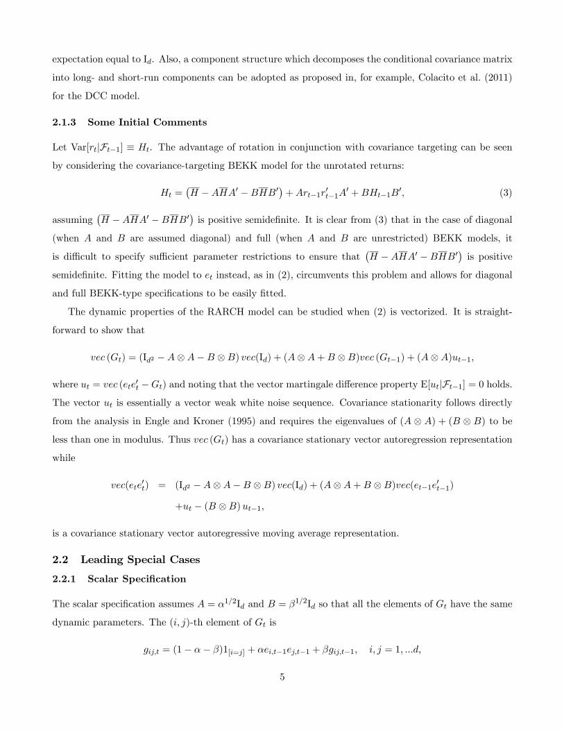
2.1.3 Some Initial Comments
Let Var[rtjFt�1] � Ht. The advantage of rotation in conjunction with covariance targeting can be seen
by considering the covariance-targeting BEKK model for the unrotated returns:
Ht =�H �AHA0 �BHB0
�+Art�1r
0t�1A
0 +BHt�1B0; (3)
assuming�H �AHA0 �BHB0
�is positive semide�nite. It is clear from (3) that in the case of diagonal
(when A and B are assumed diagonal) and full (when A and B are unrestricted) BEKK models, it
is di¢ cult to specify su¢ cient parameter restrictions to ensure that�H �AHA0 �BHB0
�is positive
semide�nite. Fitting the model to et instead, as in (2), circumvents this problem and allows for diagonal
and full BEKK-type speci�cations to be easily �tted.
The dynamic properties of the RARCH model can be studied when (2) is vectorized. It is straight-
forward to show that
vec (Gt) = (Id2 �AA�B B) vec(Id) + (AA+B B)vec (Gt�1) + (AA)ut�1;
where ut = vec (ete0t �Gt) and noting that the vector martingale di¤erence property E[utjFt�1] = 0 holds.
The vector ut is essentially a vector weak white noise sequence. Covariance stationarity follows directly
from the analysis in Engle and Kroner (1995) and requires the eigenvalues of (A A) + (B B) to be
less than one in modulus. Thus vec (Gt) has a covariance stationary vector autoregression representation
while
vec(ete0t) = (Id2 �AA�B B) vec(Id) + (AA+B B)vec(et�1e0t�1)
+ut � (B B)ut�1;
is a covariance stationary vector autoregressive moving average representation.
2.2 Leading Special Cases
2.2.1 Scalar Speci�cation
The scalar speci�cation assumes A = �1=2Id and B = �1=2Id so that all the elements of Gt have the same
dynamic parameters. The (i; j)-th element of Gt is
gij;t = (1� �� �)1[i=j] + �ei;t�1ej;t�1 + �gij;t�1; i; j = 1; :::d;
5

where 1[�] is the indicator function. Here we assume �; � � 0. Note that if � = 0, � is unidenti�ed and
needs to be set equal to zero indicating conditional homoskedasticity in the model. Covariance stationarity
requires �+ � < 1.
2.2.2 Diagonal Speci�cation
In the diagonal speci�cation, A and B are assumed to be diagonal with elements �1=2ii and �1=2ii , i = 1; :::d.
This speci�cation implies
gij;t = (1� �1=2ii �1=2jj � �1=2ii �
1=2jj )1[i=j] + �
1=2ii �
1=2jj ei;t�1ej;t�1 + �
1=2ii �
1=2jj gij;t�1; i; j = 1; :::d:
We assume �1=2ii ; �1=2ii � 0.6 The cross-equation parameter restrictions between the variance and covari-
ance equations are a feature of BEKK-type parameterizations. Covariance stationarity is determined by
the eigenvalues of the diagonal matrix:
AA+B B =
0BBBB@�1=211 A+ �
1=211 B 0 � � � 0
0 �1=222 A+ �
1=222 B
. . ....
.... . . . . . 0
0 � � � 0 �1=2dd A+ �
1=2dd B
1CCCCA :
De�ne
�ij = �1=2ii �
1=2jj + �
1=2ii �
1=2jj ;
which we call �persistence parameters�as they control the persistence of Gt. Obviously �ij = �ji so that
AA+B B has d(d+ 1)=2 unique elements. To ensure covariance stationarity, we impose
max�ij < 1; i; j = 1; :::d: (4)
Note that this restriction also ensures that Id�AA0�BB0 is positive de�nite which highlights the particular
advantage of the RARCH model. In practice, imposing �ii = �ii + �ii < 1, by parameterizing the model
in terms of �ii and �ii, is a necessary and su¢ cient condition for (4) to hold; see Engle and Kroner (1995).
It will be convenient to introduce measures of the heterogeneity of the smoothness and persistence
parameters in the elements of Gt. By smoothness parameters we refer to the coe¢ cients �ii for gii;t and
�1=2ii �
1=2jj for gij;t, while �ii and �ij determine the persistence of gii;t and gij;t, respectively. For ease of
interpretation, we focus only on the smoothness and persistence parameters for gii;t (i.e. the conditional
6 It is worth noting that Engle and Kroner (1995) did not impose non-negativity restrictions on the elements of A and B,except for restricting their �rst elements, �1=211 and �1=211 , to be positive for identi�cation. This allows for the possibilities of(i) a positive cross product of returns decreasing the conditional covariance, and (ii) an oscillatory path for the conditionalcovariance/correlation. By assuming �1=2ii ; �
1=2ii � 0 we rule out such possibilities.
6

variances), noting that the dynamic parameters of gij;t are linked to those of gii;t and gjj;t as shown above.
Let
�� = d�1
dXi=1
�ii
denote the mean estimate of �ii, and
�� =
vuutd�1 dXi=1
(�ii � ��)2
be a corresponding measure of heterogeneity. We similarly de�ne �� and �� for �ii, and �� and �� for
�ii. Note that for the scalar model, �� = �� = �� = 0. These measures are useful for motivating the
common persistence speci�cation, as well as introducing empirical Bayes estimation in Section 3.2.
2.2.3 Common Persistence Speci�cation
In the diagonal case, (A A) + (B B) will be a diagonal matrix with diagonal elements given by
�ij = �1=2ii �
1=2jj + �
1=2ii �
1=2jj . We propose a new speci�cation in the context of diagonal structures, which
we call the common persistence (CP) speci�cation. The CP speci�cation imposes
�ij = �; 8i; j = 1; :::; d;
implying AA+B B = �Id2 . This gives the dynamic equation
Gt = (1� �)Id +A(et�1e0t�1 �Gt�1)A0 + �Gt�1; (5)
where A is a diagonal matrix with elements �1=2ii � 0, and 0 < � < 1 is a scalar parameter satisfying
� � max�ii. This implies
gij;t = (1� �)1[i=j] + �1=2ii �
1=2jj ei;t�1ej;t�1 + (�� �
1=2ii �
1=2jj )gij;t�1; i; j = 1; :::d;
The CP speci�cation has d + 1 dynamic parameters compared to 2d dynamic parameters in the
diagonal model. It imposes common persistence on all elements of Gt through a common eigenvalue, �,
for the dynamic equation for Gt.7 The condition for covariance stationarity is simply � < 1, which also
guarantees that (1��)Id is positive de�nite. This speci�cation allows the di¤erent elements of Gt to load
freely on the lagged variances/covariances and the corresponding shocks allowing them to have di¤erent
smoothness levels; however it restricts them to have common persistence through �. In contrast to the
diagonal speci�cation, here we have �� = 0, while �� 6= 0 which also implies �� 6= 0.7More generality can be introduced in (5) by assuming Gt = (Id � e�e�0) + A(et�1e0t�1 � Gt�1)A0 + e�Gt�1e�0, where e� is
diagonal matrix with a block structure such that di¤erent groupings of assets have di¤erent persistence levels.
7

GARCH(1,1): alpha IQRGARCH(1,1): beta IQRGARCH(1,1): lambda IQRComponent GARCH: rho IQR
2004 2005 2006 2007 2008 2009
0.05
0.10
0.15
0.20
0.25
0.30
0.35
0.40 GARCH(1,1): alpha IQRGARCH(1,1): beta IQRGARCH(1,1): lambda IQRComponent GARCH: rho IQR
Figure 1: Heterogeneity in the smoothness and persistence parameters of the GARCH(1,1) model and the component GARCHmodel of Engle and Lee (1999) for the S&P 100 stocks during the period 1/4/2000-1/12/2008. The �gure shows a time seriesof the inter-quartile range (IQR) for rolling-window estimates of the GARCH(1,1) model parameters, �ii and �ii, as well asthe persistence, �ii = �ii + �ii. The dashed black line is the IQR for rolling-window estimates of the persistence parameterin the long-run variance component, �ii, using the component GARCH model of Engle and Lee (1999). A rolling window of1,000 observations is used to estimate the parameters.
This speci�cation is motivated by the empirical observation that persistence levels in the conditional
variances of asset returns are less heterogeneous than their smoothness levels. Figure 1 shows a time series
of the inter-quartile range (IQR) for rolling-window estimates of the GARCH(1,1) model parameters, �ii
and �ii, as well as the implied persistence, �ii = �ii + �ii, for 94 stocks of the S&P 100 index which
consistently appeared on the index during the period 1/4/2000-1/12/2008.8 Before the �nancial crisis,
the IQR for �ii was noticeably lower than that for both �ii and �ii, especially compared to �ii. During the
recent �nancial crisis, more heterogeneity appears in �ii probably due to a decline in volatility persistence
for some stocks in reaction to the sudden increase in their average levels of volatility during the crisis.
However, it remains lower than the �ii IQR, and gradually returns to its pre-crisis level by the end of the
sample.
The GARCH(1,1) model is likely to miss the volatility dynamics during the crisis due to rapidly
8Here we are studying univariate GARCH models for a panel of assets as should be clear from the context. The sourceof the data is Thompson Reuters Datastream, and the stocks are listed in Appendix A. We used a rolling window of 1,000observations, about 4 years of data, to estimate the parameters.
8

changing volatility levels. To capture this feature, we also estimated the component GARCH model of
Engle and Lee (1999) using the same data. In this model the conditional variance for asset i is modelled
as hii;t = qii;t + sii;t, where
qii;t = !ii + �iiqii;t�1 + �ii(r2i;t�1 � hii;t�1);
sii;t = (�sii + �sii)sii;t�1 + �
sii(r
2i;t�1 � hii;t�1);
such that qii;t and sii;t represent the long- and short-run variance components, respectively. The short-run
component has persistence �sii+�sii where the superscripts are used in reference to the sii;t equation, while
qii;t has persistence �ii which is assumed to be larger than �sii + �
sii for identi�cation. This model is a
restricted GARCH(2,2) model and is better able to capture changes in the long-run variance over time.
We �nd the IQR for the cross-section estimates of �ii to be quite low, and although it increases during
the �nancial crisis, it remains indicative of a high degree of homogeneity in the persistence levels of the
long-run component. The IQR for �sii + �sii, not plotted in Figure 1 to improve presentation, is much
larger reaching as high as 0.763 during the crisis.
Brownlees (2010) studies a large cross section of U.S. �nancial �rms during the crisis, and �nds the
cross-sectional variation in �ii to be negligible, while smoothness tends to decline with the leverage of the
company. In the context of the DCC model, Hafner and Franses (2009) make a related observation by
arguing that heterogeneity in �ii is greater than that in �ii, and in one of their speci�cations they impose
a common smoothing parameter �.9 We conjecture that imposing a common persistence parameter, �,
is more intuitive since assets with di¤erent �ii�s are also likely to display varying levels of smoothness
through �ii. In addition, the advantage of our speci�cation is that a single parameter, �, controls both
covariance stationarity and positive de�niteness of (1��)Id regardless of the dimensionality of the system.
2.2.4 Orthogonal Parameter Matrices
Another interesting case, which we outline here but do not pursue empirically, is when A and B are made
up of orthogonal vectors
A = (a1; :::; ad); B = (b1; :::; bd)
and so �AA0
�ij= aia
0j = �ij1[i=j];
�BB0
�ij= bib
0j = �ij1[i=j]; i; j = 1; 2; :::; d:
Orthogonality of A and B implies that Id � AA0 � BB0 is diagonal, which means one can easily impose
restrictions on A and B to ensure Id �AA0 �BB0 is positive semide�nite.9 In their paper, the parameters are those of the dynamic equation for the conditional correlations; we will discuss the
DCC model in more detail in Section 2.4.
9

g11
0 200 400 600 800 1000
0.6
1.0
1.4
1.8 g11 g22
0 200 400 600 800 1000
0.8
1.0
1.2
g22
g12
0 200 400 600 800 1000
0.2
0.0
0.2
0.4 g12 Conditional correlation
200 400 600 800 1000
0.2
0.0
0.2
0.4 Conditional correlation
Figure 2: Sample path of Gt for 1,000 simulations.
Example 1 Suppose d = 2 and we parameterize A as
A =
�1=211 �c�1=211
c�1=222 �
1=222
!; Aet�1 =
�1=211
c�1=222
!e1;t�1 +
�c�1=211�1=222
!e2;t�1;
then A is orthogonal and AA0 is diagonal with �rst element �11�1 + c2
�, and second element �22
�1 + c2
�.
When c = 0 then A is diagonal. In the diagonal case suppose �1=211 = 0:300, �1=211 = 0:950, �1=222 = 0:150,
�1=222 = 0:980. Figure 2 shows the sample path of Gt for 1; 000 simulated observations assuming dynamics
similar to (2). Top left is g11;t, top right is g22;t, bottom left is g12;t while bottom right is the conditional
correlation.
Remark 1 One parameterization for A and B in the orthogonal parameters version of RARCH is to use
A = diag��1=2ii
�PA; B = diag
��1=2ii
�PB;
where �1=2ii and �1=2ii are identical to those in the diagonal speci�cation, and PA and PB are orthonormal
matrices.
10

PA can be computed using a set of d (d� 1) =2 parameters on [�1; 1]d(d�1)=2, by exploiting the relation-
ship between correlation matrices and the space of orthonormal matrices. Let the d(d� 1)=2 parameter be
denoted
�21; �31; �32; �41; �42; �43; �51; : : : ; �d(d�1)
and de�ne CA = [cij ] where
cij =
8>>>><>>>>:1 i; j = 1;q
1�Pj�1k=1 c
2ik i = j 6= 1;
�ij
q1�
Pj�1k=1 c
2ik i > j;
0 i < j:
De�ne RA = CAC 0A, and �nally PA are the eigenvectors of RA so that RA = PA�AP0A. PB can be similarly
parameterized. Finally, AA0 = diag��1=2ii
�PAP
0Adiag
��1=2ii
�= diag (�ii) and BB0 = diag (�ii), so that
the constraint needed for stationarity is that �ii+�ii < 1 for all i, which also ensures that Id�AA0�BB0
is positive de�nite.
2.3 Implied BEKK Model for rt
For the conditional covariance matrix of the unrotated returns, Ht, the RARCH model in (1) and (2)
implies that
Ht = H1=2GtH
1=2= CC
0+Art�1r
0t�1A
0+BHt�1B
0;
where
A = H1=2AH
�1=2; B = H
1=2BH
�1=2; CC
0= H
1=2 �Id �AA0 �BB0
�H1=2: (6)
It is clear that the RARCH model implies a BEKK model for rt but it is not an entirely general BEKK
model; rather it is a constrained version since A and B are rotations of A and B which depend on the
spectral decomposition of H.
Bauwens et al. (2006) discuss the invariance of multivariate GARCH models to linear transformations
of rt. In their de�nition, invariance implies that the model for the transformed series is within the same
model class (e.g. BEKK class) and retains the same dynamic speci�cation (e.g. scalar, diagonal or full
parameterization). This de�nition di¤ers from the �stability by aggregation�property discussed in Francq
and Zakoian (2010, Ch. 11), which refers only to model class invariance. Bauwens et al. (2006) note that
BEKK models are invariant to linear transformations except in the case of diagonal dynamics. For scalar
dynamics, we further note that the scalar RARCH model will have the same dynamic parameters as the
scalar BEKK model. This holds since A = �1=2Id implies A = �1=2P�1=2P 0P��1=2P 0 = �1=2Id, and the
same applies to B.
11

In the case of diagonal speci�cations, which are not invariant to linear transformations, the diagonal
RARCH model implies a full BEKK model for rt. Suppose A is diagonal, then A = P�1=2P 0AP��1=2P 0
which is a full matrix that is asymmetric in general. The same applies to B when B is diagonal. This
means that �tting a diagonal RARCH model implies rather rich dynamics for the unrotated returns.
When the asymmetric square root is used, a diagonal RARCH model implies a full BEKK for rt with
A = P�1=2A��1=2P 0 = PAP 0 which is symmetric, and B will also be symmetric. Thus, we prefer the
symmetric square root given the generality it implies for the model of the unrotated returns since A and
B will be asymmetric in this case.
2.4 The Rotated Conditional Correlation (RCC) Model
One shortcoming of the BEKK-type parameterization in the RARCH model is that the dynamics of gij;t
is linked to the dynamics of gii;t and gjj;t for all i and j through cross-equation parameter restrictions.
This is overcome if we apply the rotation to the returns after having them standardized in a �rst step by
their �tted conditional variances. This is in the spirit of the DCC model of Engle (2002), thus we call the
resulting model the rotated conditional correlation (RCC) model. As in DCC, RCC allows for the speed
of change in the conditional correlations to be di¤erent than that of the individual volatilities, and also
allows models to be �t in quite large dimensions.
Let Ht = DtCtDt where Dt = diag(phii;t). Thus Ct is the conditional correlation matrix of rt. In the
DCC model the conditional variances, Var[ri;tjFrit�1] � hii;t, i = 1; 2; :::; d, are set as univariate GARCH
processes, where Frit�1 is asset i�s own univariate information set, or �natural �ltration.�Then let
"t = D�1t rt
denote the standardized, potentially correlated returns and let their unconditional covariance be written
as
� = Var["t]:
The correlation dynamics are modelled as
Ct = (Qt � Id)�12Qt(Qt � Id)�
12 ; (7)
where � denotes the Hadamard elementwise product, with specifying a dynamic equation for Qt. For
instance, a correlation-targeting scalar DCC model is
Qt = (1� �� �)� + �"t�1"0t�1 + �Qt�1; (8)
where � and � satisfy restrictions similar to the scalar BEKK model. This ensures that Ct is a genuine
correlation matrix.
12

From (8), it is clear that a rotation of the standardized returns, "t, enables us to �t speci�cations with
�exible dynamics as demonstrated with the RARCH model for the non-standardized returns. Decompose
� = PC�CP0C where PC contains the eigenvectors and �C has the eigenvalues on the main diagonal. Then
we construct the rotated standardized returns
eet = PC��1=2C P 0C"t:
where Var[eet] = Id. Then we model the dynamics of Var[eetjFt�1] � Q�t asQ�t =
�Id �AA0 �BB0
�+Aeet�1ee0t�1A+BQ�t�1B; Q�0 = Id: (9)
As shown for the RARCH model, Qt is given by
Qt = PC�1=2C P 0CQ
�tPC�
1=2C P 0C ;
which is used to construct the correlation matrix according to (7).
Aielli (2006) points to a bias problem in the DCC model when estimating � in (8) using a moment
estimator based on "t since E["t�1"0t�1] 6= E[Qt]. The RCC model is not subject to this bias since in (9)
we have E[eet�1ee0t�1] = E[Q�t ] = Id. This is an important advantage of the RCC model.Setting A = �1=2Id and B = �1=2Id gives the scalar RCC model. We can also introduce more �exible
dynamics by allowing A and B to be diagonal or follow CP dynamics in the recursion for Q�t . The RCC
model contributes to a recent research push aiming to increase the �exibility of the DCC model; see, for
example, Cappiello et al. (2006), Billio et al. (2006), Billio and Caporin (2009) and Hafner and Franses
(2009).
The main model in Hafner and Franses (2009) bears close resemblance to a diagonal BEKK-type model
applied to (8). The primary di¤erence is that we apply this speci�cation to the rotated standardized
returns, which has the important implication that unlike Hafner and Franses (2009), our model preserves
the correlation targeting property and is also not subject to the bias problem discussed in Aielli (2006).
The CP speci�cation is also somewhat related to one of the proposed models in Hafner and Franses
(2009), the distinction being that they impose a common smoothing parameter � on the system for the
unrotated standardized returns, while we impose common persistence through � on the system for the
rotated standardized returns.
In the context of DCC models, Bauwens et al. (2011) also use the idea of orthogonalizing the daily
returns in a �rst step. There are, however, two main di¤erences between RCC and their model. First,
they �t a DCC model to the rotated returns whereas we apply the rotation to the standardized returns,
i.e. after the �rst step of �tting the conditional variances. Second, we use a constant rotation matrix for
13

"t, while they use a slowly-varying rotation matrix computed using a Nadaraya-Watson estimator applied
to rt. For future work, it would be interesting to compare the two models empirically.
2.5 Relation to Orthogonal GARCH Models
In this subsection, we discuss how the RARCHmodel di¤ers from the class of OGARCHmodels introduced
in Alexander and Chibumba (1997), and further extended and re�ned in van der Weide (2002), Lanne
and Saikkonen (2007), Fan et al. (2008) and Boswijk and van der Weide (2011) among others. Consider
general linear transformations of the form: rt = Zet, where Z is some invertible matrix. Lanne and
Saikkonen (2007) propose the polar decomposition for Z such that
Z = SU; (10)
where S is a symmetric positive de�nite matrix, and U is an orthogonal matrix. Since Var[et] = Id, we
have Var[rt] � H = ZZ 0 = S2, thus S is the symmetric square root of H given by P�1=2P 0. Therefore
part of the Z matrix can be estimated using only unconditional information.
The OGARCH model of Alexander and Chibumba (1997) and Alexander (2001) assumes U = P , hence
Z = P�1=2, which is the asymmetric square root of H. In this case et is a vector of the standardized
principal components of rt which are unconditionally uncorrelated by construction. Alexander (2001)
assumes that these standardized principal components are also conditionally uncorrelated with a diagonal
conditional covariance matrix, which gives the following dynamic equation:
Gt =�Id � eA eA0 � eB eB0�+ eA eA0 � �et�1e0t�1�+ eB eB0 �Gt�1; (11)
where eA and eB are diagonal. Its popularity in applications relates to the convenient form of (11) which
allows for estimating the diagonal elements of Gt individually as univariate GARCH models, and this
is obviously helpful in large dimensions. However, assuming that Gt is diagonal is an ad hoc restriction
and possibly a misspeci�cation since we expect the standardized principal components to inherit the
heteroskedastic properties of the original returns; Fan et al. (2008) argue similarly. The OGARCH model
completely ignores the information in the cross products of the rotated returns, and we will show that
this leads to statistically signi�cant loss of information when modelling and forecasting the conditional
correlations.
The GOGARCH model of van der Weide (2002), when modi�ed according to Boswijk and van der
Weide (2011), implies Z = SU(�) = P�1=2P 0U(�), where the orthogonal matrix U(�) is parameterized by
a d(d� 1)=2� 1 vector �, with j-th element �180 � �j � 180 which is a rotation angle. The dynamics of
the resulting et = Z�1rt are modelled as in (11).
14

Our model takes a di¤erent stand by assuming that Gt is a full matrix. Thus we include information
from the cross products of the rotated returns which are ignored in the OGARCH and GOGARCH models.
This means that our model and the OGARCH model are non-nested. With reference to (10), we simply
assume U = Id, which means that et is not a unique set of components that satis�es Var[et] = Id. For
instance, we can post-multiply H1=2
= P�1=2P 0 by an arbitrary orthogonal matrix U�, and still have
Var[et] = E[ete0t] = E[U�0H
�1=2rtr
0tH
�1=2U�] = Id. However, uniqueness (or identi�ability) of et is not
crucial since our objective is to simplify estimation, not get unique estimates of et. What is important is
that for any model for et, it is straightforward to derive the implied model for rt as shown in Section 2.3.
It is worth noting that Fan et al. (2008) make an important departure from the earlier OGARCH
models by estimating U under the condition that the resulting components, et, are also conditionally
uncorrelated. While the model of Fan et al. (2008) is conceptually appealing, a set of conditionally
uncorrelated components may not exist. Thus, in practice, their model may only give components that
are the least conditionally correlated in-sample. Boswijk and van der Weide (2011) adopt a closely
related approach to estimate conditionally uncorrelated factors, which departs from earlier work on the
GOGARCH model.
2.6 A Time-Varying-Weight Strict Factor Model Representation
The RARCH model can also be interpreted as a time-varying-weight strict factor model since it implies
Ht = H1=2GtH
1=2= P�1=2P 0GtP�
1=2P 0:
Suppose we take the spectral decomposition of Gt at each point in time such that Gt = PGt �Gt (P
Gt )
0,
where PGt contains the eigenvectors of Gt and the diagonal matrix �Gt has the eigenvalues of Gt along its
main diagonal. Then we can write
Ht = P�1=2P 0PGt �
Gt (P
Gt )
0P�1=2P 0 = zt�Gt z
0t;
where zt = P�1=2P 0PGt is a time-varying weight matrix.
This representation is reminiscent of strict factor models where the factors are not correlated, their
conditional variances are given by the diagonal elements of the time-varying �Gt , and there is no approx-
imation error covariance since the number of factors is equal to the number of assets. The term strict
factor model is typically used to characterize a model where the idiosyncratic components of asset returns
are uncorrelated as in Ross (1976), for example. Here we adapt it to describe a model where the factors
are uncorrelated both conditionally and unconditionally, and the factor loadings, zt, are time-varying.
15

Note that OGARCH models assume that Gt is diagonal, and in this case �Gt = Gt while PGt = Id, hence
they impose a �xed weight matrix z = P�1=2P 0. This representation provides an additional intuition
behind our model, and explains why capturing the covariance dynamics of ei;t, i = 1; :::; d, is important.
3 Inference and Model Evaluation
3.1 Maximum Likelihood Estimation
3.1.1 Optimization via Multisteps
For RARCH, OGARCH and GOGARCH models, let �S = vech(H) denote the model�s static parameters,
and let �D denote the vector of dynamic parameters indexing A and B in (2) for the RARCH model, or
indexing eA and eB in (11) for OGARCH and GOGARCH. The full parameter vector is � = ��0S ; �0D�0, andthe true parameter vector is denoted by �0. Typically the dimension of �S is large and potentially massive
if d is large since it has O(d2) elements. The dimension of �D is often small with only O(d) parameters
in the speci�cations we consider.
The structure of these models allows for a 2-step estimation strategy to estimate �. In the �rst step,
we use a method of moments estimator:
bH = T�1TXt=1
rtr0t;
implying b�S . This estimate is then decomposed into bP and b�. Then we construct the time series of rotatedreturns, et = bP b��1=2 bP 0rt, t = 1; 2; :::; T . The second-step estimation is based on the quasi-likelihood
logL(�D;b�S) = TXt=1
logLt(�D;b�S) = �12
TXt=1
�d log(2�) + log jGtj+ e0tG�1t et
�; (12)
where Gt is given by (2).
This is optimized over �D keeping b�S �xed, which delivers b�D. When estimating the OGARCH model,we use et = b��1=2 bP 0rt in (12) while the dynamic equation for Gt will be given by (11). For GOGARCHwe use et = bP b��1=2 bP 0rt in the following quasi-likelihood
logL(�D;b�S) = TXt=1
logLt(�D;b�S) = �12
TXt=1
�d log(2�) + log jGtj+ e0tU(�)G�1t U(�)0et
�;
where the dynamic equation for Gt is also given by (11). In the GOGARCH case, the additional d(d�1)=2
parameters in � are contained in �D.10
10When d is large, estimating � is generally challenging thus we only include the GOGARCH model for comparison in ourempirical analysis in the bivariate case.
16

Remark 2 The GOGARCH model uses a di¤erent rotation than the RARCH model, unless � = 0, and
so the di¤erence between the two is not only due to the non-zero conditional covariances in the RARCH
model. Eq. (12) could be modi�ed to allow for an estimated rotation matrix by modifying the �nal term
to be e0tU(�)G�1t U(�)
0et which would not pose an identi�cation problem since the long-run covariance is
Id. We do not pursue this parameterization further since estimating the d(d � 1)=2 parameters of U(�)
substantially increases the computational burden, except when d is small.
For the RCC model, let e�M = (e�01; :::;e�0d)0 denote the parameter vector of the d marginal models,e�S = vech(�) where � is the unconditional covariance of the standardized returns, "t, and e�D is the
vector of dynamic parameters in (9). The full parameter vector is e� = (e�M ;e�S ;e�D), and the true parametervector is denoted by e�0. The log-likelihood is
logL(e�M ;e�S ;e�D) =
TXt=1
logLt(e�M ;e�S ;e�D)=
TXt=1
dXi=1
logLi;t(e�i) + TXt=1
logLC;t(e�M ;e�S ;e�D). (13)
where logLi;t(�) and logLC;t(�) denote the i-th margin and correlation log-likelihoods respectively. The
two terms in (13) can be written as
TXt=1
dXi=1
logLi;t(e�i) = �12
TXt=1
�d log(2�) + 2 log jDtj+ r0tD�2t rt
�TXt=1
logLC;t(e�M ;e�S ;e�D) = �12
TXt=1
��"0t"t + log jCtj+ "0tC�1t "t
�.
3.1.2 Asymptotic Distribution
To compute asymptotic standard errors, we cast the estimators into a method of moments frame-
work. For RARCH, OGARCH and GOGARCH models, the moment conditions for the t-th observa-
tion are given by mt = (m0S;t;m
0D;t)
0, where mS;t = �S � vech (rtr0t) and mD;t =@ logLt(�S ;�D)
@�D. For
RCC, the moment conditions for the t-th observation are given by emt = (em0M;t; em0
S;t; em0D;t)
0, where
emM;t =
�@ logL1;t(e�1)
@e�1 ; :::;@ logLd;t(e�d)
@e�d�collects the scores of the marginal models, emS;t = e�S � vech ("t"0t)
and emD;t =@ logLC;t(e�M ;e�S ;e�D)
@e�D .
It holds that E [mtjFt�1] = 0 and E [emtjFt�1] = 0 at the true parameter values. In terms of asymptotic
theory, for �xed d and T ! 1, this is simply a 2-step moment estimator, e.g. Newey and McFadden
(1994) and Pagan (1986), in the case of RARCH, OGARCH and GOGARCH. In the case of RCC, this is
17
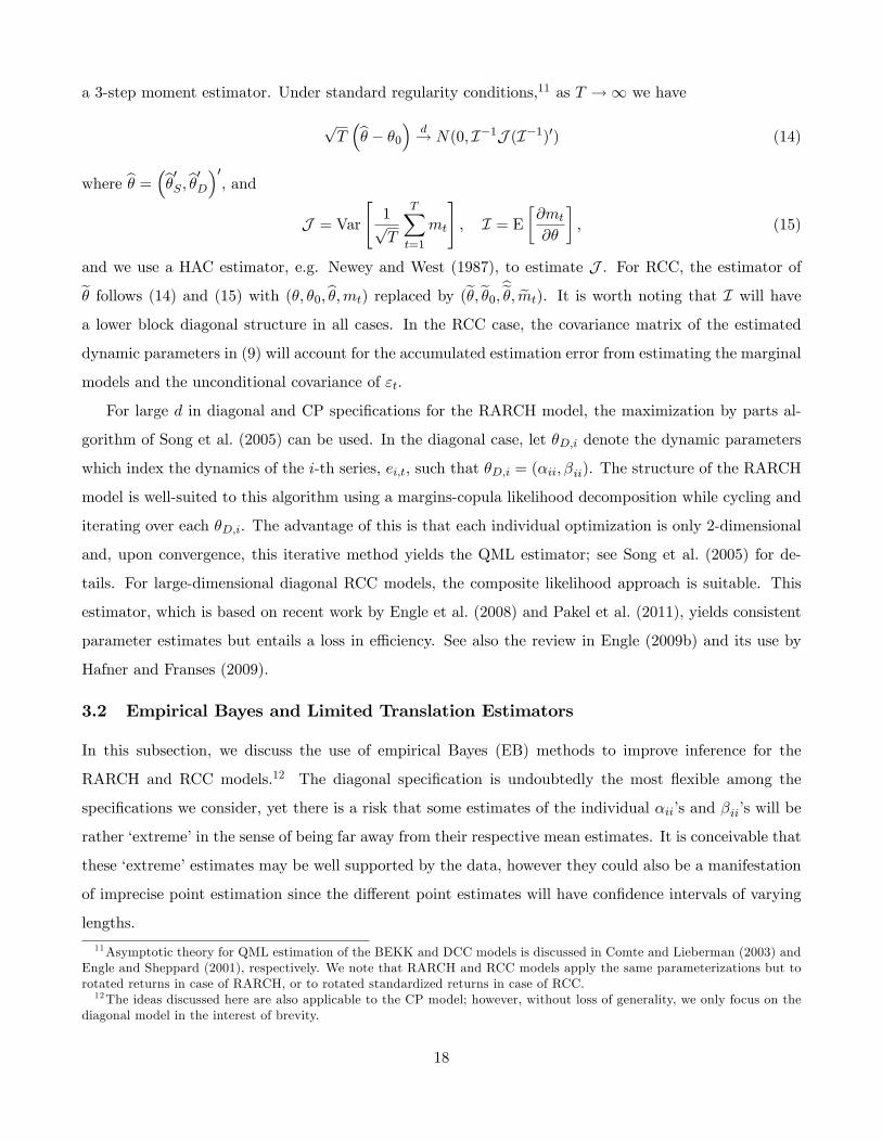
a 3-step moment estimator. Under standard regularity conditions,11 as T !1 we have
pT�b� � �0� d! N(0; I�1J (I�1)0) (14)
where b� = �b�0S ;b�0D�0, andJ = Var
"1pT
TXt=1
mt
#; I = E
�@mt
@�
�; (15)
and we use a HAC estimator, e.g. Newey and West (1987), to estimate J . For RCC, the estimator ofe� follows (14) and (15) with (�; �0;b�;mt) replaced by (e�;e�0;be�; emt). It is worth noting that I will have
a lower block diagonal structure in all cases. In the RCC case, the covariance matrix of the estimated
dynamic parameters in (9) will account for the accumulated estimation error from estimating the marginal
models and the unconditional covariance of "t.
For large d in diagonal and CP speci�cations for the RARCH model, the maximization by parts al-
gorithm of Song et al. (2005) can be used. In the diagonal case, let �D;i denote the dynamic parameters
which index the dynamics of the i-th series, ei;t, such that �D;i = (�ii; �ii). The structure of the RARCH
model is well-suited to this algorithm using a margins-copula likelihood decomposition while cycling and
iterating over each �D;i. The advantage of this is that each individual optimization is only 2-dimensional
and, upon convergence, this iterative method yields the QML estimator; see Song et al. (2005) for de-
tails. For large-dimensional diagonal RCC models, the composite likelihood approach is suitable. This
estimator, which is based on recent work by Engle et al. (2008) and Pakel et al. (2011), yields consistent
parameter estimates but entails a loss in e¢ ciency. See also the review in Engle (2009b) and its use by
Hafner and Franses (2009).
3.2 Empirical Bayes and Limited Translation Estimators
In this subsection, we discuss the use of empirical Bayes (EB) methods to improve inference for the
RARCH and RCC models.12 The diagonal speci�cation is undoubtedly the most �exible among the
speci�cations we consider, yet there is a risk that some estimates of the individual �ii�s and �ii�s will be
rather �extreme�in the sense of being far away from their respective mean estimates. It is conceivable that
these �extreme�estimates may be well supported by the data, however they could also be a manifestation
of imprecise point estimation since the di¤erent point estimates will have con�dence intervals of varying
lengths.
11Asymptotic theory for QML estimation of the BEKK and DCC models is discussed in Comte and Lieberman (2003) andEngle and Sheppard (2001), respectively. We note that RARCH and RCC models apply the same parameterizations but torotated returns in case of RARCH, or to rotated standardized returns in case of RCC.12The ideas discussed here are also applicable to the CP model; however, without loss of generality, we only focus on the
diagonal model in the interest of brevity.
18

The structure of the RARCH and RCC models makes the use of empirical Bayes a natural extension.
Suppose that in the diagonal speci�cation the shock parameters (�ii�s) and smoothing parameters (�ii�s)
are drawn from distributions that are centred around corresponding scalar parameters. Given this prior
and the point estimates from QML estimation, denoted by �MLii and �MLii , we can use EB methods to
make inference about the posterior distribution of the parameters having observed �MLii and �MLii . For a
recent overview of empirical Bayes methods, see Efron (2010).
Since the shrinkage will be applied di¤erently to the �ii�s and �ii�s, in what follows we use ii to
generically denote either parameter. Assume the following prior distribution: iii:i:d:� N(� ; � ).
13 The
ML estimator being consistent and asymptotically normal implies MLii j ii�� N( ii; �
2 ii). Noting that
estimates of �2 ii are available from QML estimation, then the posterior distribution of ii is14
iij MLii�� N
0@� + � �� + �2 ii
� � MLii � � �;
� �2 ii�
� + �2 ii
�1A ;
which depends on the unknown parameters � and � . The EB estimator utilizes the information in MLii
to make inference about these parameters. De�ne
= d�1Xd
i=1 MLii ;
then the EB estimator is
EBii = +
0B@1� (d� 3)�2 iiXd
i=1( MLii � )2
1CA� MLii � �: (16)
This EB estimator is itself the James and Stein (1961) shrinkage estimator. James and Stein (1961)
showed that it everywhere dominates the ML estimator in terms of estimation risk under quadratic loss
for dimensions larger than or equal to three. Empirical Bayes estimators utilize these shrinkage gains and
they have proven useful in many applications; Morris (1983) and Efron (2010) provide overviews of the
main results and discuss some applications. Here the Stein e¤ect works for d � 4 because of the need to
estimate � by the sample average, .
Of course, the EB method is related to the heterogeneity of the dynamic and persistence parameters
as discussed in Section 2.2.2 to motivate the CP speci�cation. It is clear from (16) that the EB estimator
can shrink some parameters drastically if they are far away from the mean estimate and have a relatively
13 Independence among the ii�s is a simplifying assumption which enables us to utilize the empirical Bayes estimator inits classical formulation. The alternative route of utilizing the covariance between the QML estimates would complicate thederivation of the posterior distribution.14See Efron (2010) for details.
19

large variance, �2 ii . To control for this e¤ect, Efron and Morris (1972) introduced the limited translation
(LT) estimator:
LTii =
�max( EBii ;
MLii �D� ii) for MLii > ;
min( EBii ; MLii +D� ii) for MLii � ; (17)
where D is a choice parameter. For instance, D = 1 means that LTii will never deviate more than � ii
from MLii . We will use the EB and LT estimators to assess the poolability of the dynamic parameters as
they are shrunk towards a vector of parameters that is possibly close to, but not as extreme as the scalar
speci�cation.
3.3 Model Evaluation
3.3.1 Non-Nested Comparison via Predictive Ability
We use a quasi-likelihood criterion for rt to compare the forecasts of the RARCH, OGARCH, GOGARCH
and RCCmodels, which means we will focus on the 1-step predictive ability of the models using a Kullback-
Leibler distance. Given the likelihood for et in the RARCH, OGARCH and GOGARCH models, it is
straightforward to compute the likelihood for rt since the Jacobian of the transformation is @rt@et= P�1=2P 0,
and its determinant is��P�1=2P 0�� = ���1=2��, where the second equality follows from P being orthogonal.
Thus for a time series of length T , we have logLr = logLe+ T2 log j�j, where logLr and logLe denote the
log-likelihoods for rt and et, respectively. For the RCC model, we have logL" = logLee + T2 log j�C j, and
logLr is computed by adding the sum of the log-likelihoods of the marginal models for the conditional
variances.
Let logLar;t denote the t-th observation log-likelihood for rt based on model a. To compare two models,
a and b, we look at the average log-likelihood di¤erence
la;b =1
T
TXt=1
la;b;t; la;b;t = logLar;t � logLbr;t: (18)
We then test if la;b is statistically signi�cantly di¤erent from zero by computing a HAC estimator of
the variance of la;b. This predictive ability test was introduced by Diebold and Mariano (1995). Using
a quasi-likelihood criterion is valid for non-nested and misspeci�ed models; see Cox (1961) and Vuong
(1989) for in-sample model comparison, and Amisano and Giacomini (2007) for out-of-sample model
selection. For the set of models under comparison, we choose the diagonal speci�cation within each class
(RARCH, OGARCH, GOGARCH and RCC) since it is the most �exible speci�cation, and then test for
equal predictive ability. We will use either OGARCH or GOGARCH in a comparison, but not both since
the GOGARCH nests OGARCH and thus this test would not be appropriate.15
15 If interest is in testing nested models, the approach of Giacomini and White (2006) can be adopted by using rolling-window estimation. This allows for pairwise comparisons of the predictive ability of all the four classes of models as well asthe di¤erent speci�cations under each class.
20

3.3.2 Margin-Copula Predictive Likelihood Decomposition
Noureldin et al. (2011) propose a margins-copula predictive likelihood decomposition to assess the �t of
multivariate volatility models by separating the gains/losses due to the forecast variances and correla-
tions. Let logLi =PTt=1 log f(ri;tjFt�1) be the marginal log-likelihood for the i-th asset, where we have
conditioned on the entire �ltration, not just its own natural �ltration. The copula log-likelihood is then
given by logLr �Pdi=1 logLi, where logLr is the model�s joint log-likelihood. Under the assumption of
conditional normality for rt, the copula parameter is the conditional correlation matrix of the unrotated
returns. This decomposition appears naturally in the RCC model due to the separate estimation of the
margins in a �rst step, and here we apply it to the RARCH, OGARCH and GOGARCH models. Margin-
based and copula-based predictive ability tests can be conducted as outlined in Noureldin et al. (2011).
These tests are useful to show the improvement of RARCH and RCC over OGARCH/GOGARCH in
terms of predictive power for the conditional correlations.
4 Empirical Analysis
4.1 Data
We use close-to-close daily returns data on ten stocks from the DJIA index. These are: Alcoa (AA),
American Express (AXP), Bank of America (BAC), Coca Cola (KO), Du Pont (DD), General Electric
(GE), International Business Machines (IBM), JP Morgan (JPM), Microsoft (MSFT), and Exxon Mobil
(XOM). The sample period is 1/2/2001 to 31/12/2009 and the source of the data is Yahoo!Finance, which
is accessible online. We use close prices adjusted for dividends and splits.
Our primary empirical example in Section 4.3 focuses on the pair XOM-AA, which we use to present
the models�main features. In Section 4.4 we estimate the models using all 10 stocks from the DJIA index.
4.2 Competing Models
For RARCH models, where the dynamic equation is given by (2), we �t the following speci�cations:
� Scalar RARCH (S-RARCH). A = �1=2Id and B = �1=2Id.
� Diagonal RARCH (D-RARCH). A = diag(�1=2ii ) and B = diag(�1=2ii ).
� Common persistence RARCH (CP-RARCH). A = diag(�1=2ii ) and � is the common persistence
parameter.
For comparison, we also report results for these three speci�cations when applied to OGARCH and
GOGARCH models, where in the latter models it is assumed that Gt is diagonal. The diagonal OGARCH
21
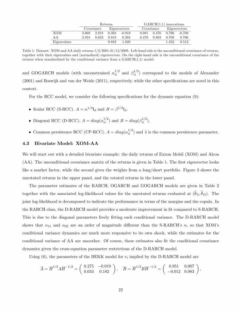
Returns GARCH(1,1) innovationsCovariance Eigenvectors Covariance Eigenvectors
XOM 3.069 2.918 0.394 -0.919 0.981 0.470 0.706 -0.708AA 2.918 8.633 0.919 0.394 0.470 0.983 0.708 0.706Eigenvalues 9.882 1.820 1.452 0.512
Table 1: Dataset: XOM and AA daily returns 1/2/2001-31/12/2009. Left-hand side is the unconditional covariance of returns,together with their eigenvalues and (normalized) eigenvectors. On the right-hand side is the unconditional covariance of thereturns when standardized by the conditional variance from a GARCH(1,1) model.
and GOGARCH models (with unconstrained �1=2ii and �1=2ii ) correspond to the models of Alexander
(2001) and Boswijk and van der Weide (2011), respectively, while the other speci�cations are novel in this
context.
For the RCC model, we consider the following speci�cations for the dynamic equation (9):
� Scalar RCC (S-RCC). A = �1=2Id and B = �1=2Id.
� Diagonal RCC (D-RCC). A = diag(�1=2ii ) and B = diag(�1=2ii ).
� Common persistence RCC (CP-RCC). A = diag(�1=2ii ) and � is the common persistence parameter.
4.3 Bivariate Model: XOM-AA
We will start out with a detailed bivariate example: the daily returns of Exxon Mobil (XOM) and Alcoa
(AA). The unconditional covariance matrix of the returns is given in Table 1. The �rst eigenvector looks
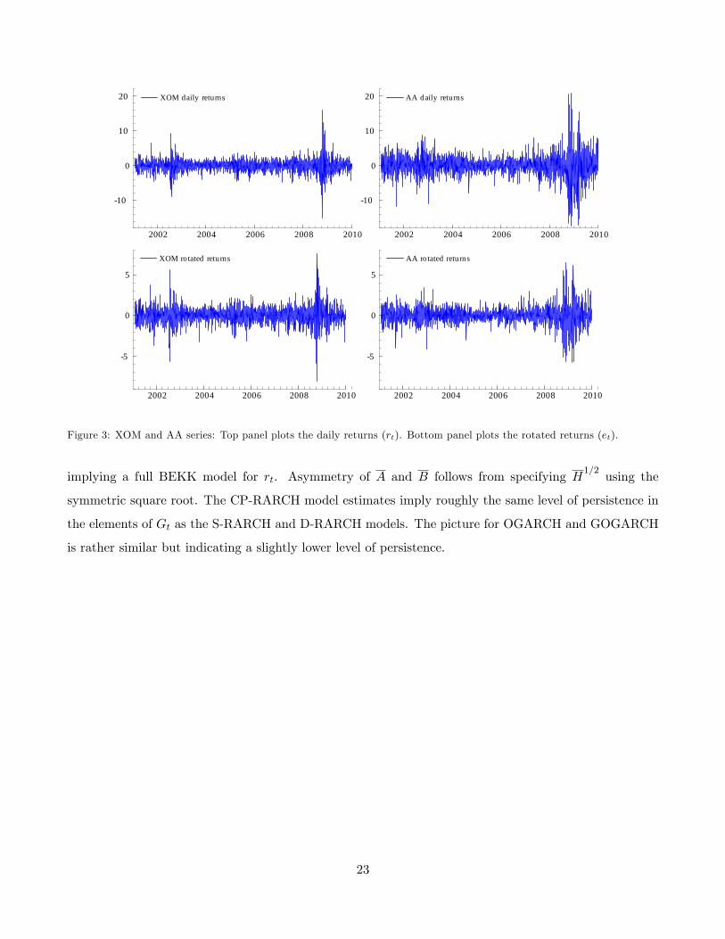
like a market factor, while the second gives the weights from a long/short portfolio. Figure 3 shows the
unrotated returns in the upper panel, and the rotated returns in the lower panel.
The parameter estimates of the RARCH, OGARCH and GOGARCH models are given in Table 2
together with the associated log-likelihood values for the unrotated returns evaluated at (b�S ;b�D). Thejoint log-likelihood is decomposed to indicate the performance in terms of the margins and the copula. In
the RARCH class, the D-RARCH model provides a moderate improvement in �t compared to S-RARCH.
This is due to the diagonal parameters freely �tting each conditional variance. The D-RARCH model
shows that �11 and �22 are an order of magnitude di¤erent than the S-RARCH�s �, so that XOM�s
conditional variance dynamics are much more responsive to its own shock, while the estimates for the
conditional variance of AA are smoother. Of course, these estimates also �t the conditional covariance
dynamics given the cross-equation parameter restrictions of the D-RARCH model.
Using (6), the parameters of the BEKK model for rt implied by the D-RARCH model are
A = H1=2AH
�1=2=
�0:275 �0:0190:034 0:182
�; B = H
1=2BH
�1=2=
�0:951 0:007�0:012 0:983
�;
22
XOM daily returns
2002 2004 2006 2008 2010
10
0
10
20 XOM daily returns AA daily returns
2002 2004 2006 2008 2010
10
0
10
20 AA daily returns
XOM rotated returns
2002 2004 2006 2008 2010
5
0
5
XOM rotated returns AA rotated returns
2002 2004 2006 2008 2010
5
0
5
AA rotated returns
Figure 3: XOM and AA series: Top panel plots the daily returns (rt). Bottom panel plots the rotated returns (et).
implying a full BEKK model for rt. Asymmetry of A and B follows from specifying H1=2
using the
symmetric square root. The CP-RARCH model estimates imply roughly the same level of persistence in
the elements of Gt as the S-RARCH and D-RARCH models. The picture for OGARCH and GOGARCH
is rather similar but indicating a slightly lower level of persistence.
23

RARCH
OGARCH
GOGARCH
RCC
SD
CP
SD
CP
SD
CP
SD
CP
Marginalparameters
�XOM
0:084
(0:015)
0:084
(0:015)
0:084
(0:015)
�XOM
0:901
(0:019)
0:901
(0:019)
0:901
(0:019)
�AA
0:048
(0:014)
0:048
(0:014)
0:048
(0:014)
�AA
0:948
(0:017)
0:948
(0:017)
0:948
(0:017)
Dynamicparameters
�0:050
(0:011)
0:066
(0:017)
0:063
(0:017)
0:015
(0:019)
�0:943
(0:013)
0:924
(0:020)
0:927
(0:022)
0:977
(0:006)
�11
0:072
(0:015)
0:055
(0:013)
0:060
(0:019)
0:076
(0:023)
0:088
(0:016)
0:067
(0:019)
0:006
(0:012)
0:005
(0:008)
�22
0:036
(0:008)
0:044
(0:010)
0:082
(0:020)
0:059
(0:016)
0:041
(0:012)
0:055
(0:020)
0:037
(0:107)
0:054
(0:062)
�11
0:909
(0:020)
0:934
(0:022)
0:884
(0:023)
0:993
(0:075)
�22
0:960
(0:009)
0:887
(0:029)
0:955
(0:014)
0:960
(0:068)
�0:993
(0:003)
0:989
(0:005)
0:991
(0:005)
0:992
(0:017)
�0:015
(0:040)
�0:008
(0:073)
0:030
(0:379)
LLdecomposition
Margin(XOM)
-4,034
-4,030
-4,032
-4,028
-4,031
-4,027
-4,029
-4,030
-4,028
-4,026
-4,026
-4,026
Margin(AA)
-5,098
-5,098
-5,099
-5,099
-5,126
-5,102
-5,100
-5,097
-5,099
-5,096
-5,096
-5,096
Copula
284
288
284
233
270
235
258
266
258
306
307
307
TotalLL
-8,848
-8,840
-8,847
-8,894
-8,887
-8,893
-8,870
-8,861
-8,869
-8,816
-8,815
-8,815
Table2:
Dataset:XOMandAAdaily
returns1/2/2001-31/12/2009.
Parameterestimatesofthescalar(S),diagonal(D)andcommon
persistence(CP)
speci�cations.Top
panel:MarginalparameterestimatesareofthevariancetargetingGARCH(1,1)modelsfortheRCCmargins.Dynamicparametersare
estimatesoftheRARCH,OGARCHandGOGARCHmodels,andthecorrelationdynamicsforRCC.�isthecommon
persistenceparameter,while�isthe
rotationangleintheGOGARCHmodel.Standarderrorsarereportedinparentheses.Bottompanel:Log-likelihooddecompositionattheestimatedparameter
values.
24

Interestingly, the GOGARCH model�s estimated rotation angle is very close to zero and statistically
insigni�cant. This implies that U(�) � Id, making the et series from the GOGARCH model very close
to those from the RARCH model. The primary di¤erence, in this case, between the two models is that
GOGARCH assumes that g12;t is zero, which is re�ected in RARCH�s superior copula �t.
The RARCH models provide an increase in the likelihood compared to OGARCH and GOGARCH.
The increase in the log-likelihood in RARCH models is primarily due to an increase in the copula �t,
implying that capturing the conditional correlations in the rotated returns (which is not the case in
OGARCH and GOGARCH) does improve the modelling of the conditional correlations of the unrotated
returns. There is a small loss in �t in the �rst margin (XOM) when using the RARCH model, however this
is more than compensated through capturing the conditional correlation dynamics with RARCH models
providing an overall gain in �t.
The last three columns of table 2 give estimates of the di¤erent RCC speci�cations. When estimating
the variance targeting GARCH(1,1) models for the margins, we �rst standardize the returns of XOM
and AA by their respective unconditional variances, �t variance targeting GARCH(1,1) models for these
standardized returns and report the log-likelihood for the original returns as the marginal log-likelihood.
The estimates suggest di¤erent dynamics for the two series, which can already be inferred from the
improvement o¤ered by the diagonal RARCH, OGARCH and GOGARCH speci�cations.
The estimates for the RCC dynamics suggest only a marginal improvement by the D-RCC and CP-
RCC over S-RCC. With the margins �t freely, there seems to be no additional improvement from further
enriching the RCC dynamics in this case. This is in contrast to the RARCH model results, but it is
perhaps unsurprising since there is a single conditional correlation to �t in this case. Overall the estimates
suggest that the conditional correlation matrix is quite persistent. The log-likelihood decomposition
results indicate a rather signi�cant improvement in the overall �t compared to the RARCH, OGARCH
and GOGARCH models, especially in comparison to OGARCH.
We apply the 1-step predictive ability test outlined in Section 3.3 to the D-RARCH, D-OGARCH
and D-RCC models which are the most �exible in each class. Comparing D-RARCH to D-OGARCH
gives a t-statistic of 2.81 which is statistically signi�cant at 1 percent, indicating that D-RARCH provides
superior 1-step forecasts. Comparing D-RCC to D-RARCH and D-OGARCH gives t-statistics equal to
2.24 and 3.74, respectively, indicating that D-RCC outperforms both models. For the correlation gains,
the t-statistics of the copula-based predictive ability tests are 1.04 for D-RARCH versus D-OGARCH,
and 1.8 and 2.4 for D-RCC versus D-OGARCH and D-RARCH, respectively.
Figure 4 plots the conditional correlations from the diagonal models which provided the best �t in each
25

DRARCHDOGARCHDRCC
2001 2002 2003 2004 2005 2006 2007 2008 2009 2010
0.1
0.2
0.3
0.4
0.5
0.6
0.7
0.8
0.9DRARCHDOGARCHDRCC
Figure 4: Conditional correlations from the diagonal RARCH, OGARCH and RCC models.
model class. The D-RCC conditional correlation is the most persistent and lies within a tighter range.
It appears to be generally lower than the conditional correlation from the D-RARCH and D-OGARCH
model, with the exception of the year 2005 where D-OGARCH conditional correlation was noticeably
lower. This observation is perhaps most evident during the latter part of the �nancial crisis, roughly
starting 2009, with a large di¤erence in the level of the conditional correlations.
4.4 10-Dimensional Model
In this subsection we analyze all 10 stocks from the DJIA index. The �rst two eigenvectors, corresponding
to the two largest eigenvalues of the unconditional covariance matrix of the returns, are reported in Table
3. The �rst eigenvector looks roughly like a market factor and the second is a market portfolio that is
short (long) in �nancial stocks (BAC, JPM and AXP) and long (short) in the other stocks.16 The two
largest eigenvalues are 35.93 and 6.85, and they account for 73 percent of the total variation in the returns,
where total variation is measured by the trace of H.
Table 4 shows the estimated parameters for the scalar, diagonal and common persistence models.
16Note that when the eigenvalues are distinct, the eigenvectors are unique up to sign.
26

BAC JPM IBM MSFT XOM AA AXP DD GE KOEigenvector 1 0.505 0.439 0.182 0.218 0.180 0.360 0.392 0.242 0.292 0.106Eigenvector 2 -0.584 -0.288 0.177 0.259 0.255 0.582 -0.033 0.223 0.077 0.129
Table 3: Dataset: 10 DJIA stocks daily returns 1/2/2001-31/12/2009. The �rst two (normalized) eigenvectors correspondto the two largest eigenvalues of the unconditional covariance matrix of the returns.
Moving from the scalar to the diagonal models seems to pay o¤ with a considerable improvement in
overall �t in D-RARCH, and less so for D-OGARCH. The RARCH models provide a signi�cant overall
gain in the log-likelihood over OGARCH, all due to improving the copula �t. Note that RARCH loses in
the margins to OGARCH as the RARCH parameters provide a �t to both the variance and covariance
elements of Gt.
Of course, the RCC models provide the best �t since the margins are freely estimated. The overall
gain compared to RARCH and OGARCH is quite impressive, and the RCC gains are uniform across
all margins and the copula. Unlike RARCH and OGARCH cases, moving from S-RCC to D-RCC does
not improve the copula �t massively. In this moderately large dimension, the favourable performance of
the CP speci�cation is evident, particularly in the RCC model where moving from D-RCC to CP-RCC
decreases the log-likelihood only marginally.
Given that both the scalar and CP speci�cations are nested in the diagonal model, we can use a
likelihood ratio (LR) test. The scalar speci�cation imposes 2d restrictions on the diagonal model, and
according to the LR test, the reduction in �t is statistically signi�cant at 5 percent in all three models.
The CP speci�cation imposes d(d + 1)=2 restrictions on the parameters of the diagonal model, and the
loss in �t when moving from D-RARCH to CP-RARCH is statistically signi�cant at 5 percent, while this
is not the case in the OGARCH and RCC models. This suggests that common persistence dynamics is
not a restrictive assumption in the OGARCH and RCC cases.
This is an interesting result since the number of dynamic parameters in the CP model is d+1 compared
to 2d dynamic parameters in the diagonal model. This is potentially due to di¤erences in the heterogeneity
of the persistence parameters, �ii, among the RARCH, OGARCH and RCC diagonal speci�cations. We
�nd that �� = 0:011 for D-RARCH, �� = 0:008 for D-OGARCH and �� = 0:019 for D-RCC implying that
common persistence may not be a reasonable assumption for RCC; however, we note that the D-RCC
parameters are subject to con�dence intervals of varying lengths and that is why the empirical Bayes
analysis adds further insight into the poolability of the dynamic parameters, as we discuss later. It is also
worth noting that �� = 0:014 and �� = 0:023 for D-RARCH, �� = 0:020 and �� = 0:026 for D-OGARCH,
and �� = 0:004 and �� = 0:020 for D-RCC.
Compared to the D-OGARCH speci�cations, D-RARCH produces superior 1-step forecasts with a
27

RARCH OGARCH RCCS D CP S D CP S D CP
Dynamic parameters� 0:020
(0:002)0:045(0:009)
0:007(0:007)
� 0:978(0:003)
0:952(0:010)
0:980(0:007)
min�ii 0:009(0:002)
0:010(0:002)
0:027(0:015)
0:025(0:009)
0:003(0:003)
0:002(0:003)
max�ii 0:054(0:017)
0:054(0:009)
0:097(0:121)
0:095(0:018)
0:018(0:022)
0:015(0:021)
min�ii 0:905(0:035)
0:869(0:177)
0:925(0:079)
max�ii 0:989(0:003)
0:967(0:020)
0:993(0:028)
� 0:998(0:001)
0:996(0:002)
0:987(0:018)
LL decompositionMargin (BAC) -4,496 -4,355 -4,373 -4,416 -4,351 -4,361 -4,350 -4,350 -4,350Margin (JPM) -4,769 -4,719 -4,734 -4,706 -4,695 -4,700 -4,671 -4,671 -4,671Margin (IBM) -4,058 -4,085 -4,092 -4,025 -4,025 -4,023 -4,011 -4,011 -4,011Margin (MSFT) -4,449 -4,488 -4,482 -4,438 -4,431 -4,433 -4,424 -4,424 -4,424Margin (XOM) -4,090 -4,067 -4,084 -4,040 -4,032 -4,035 -4,026 -4,026 -4,026Margin (AA) -5,115 -5,130 -5,132 -5,097 -5,097 -5,096 -5,096 -5,096 -5,096Margin (AXP) -4,665 -4,648 -4,652 -4,620 -4,705 -4,654 -4,599 -4,599 -4,599Margin (DD) -4,249 -4,310 -4,299 -4,231 -4,247 -4,232 -4,228 -4,228 -4,228Margin (GE) -4,291 -4,299 -4,300 -4,263 -4,327 -4,314 -4,257 -4,257 -4,257Margin (KO) -3,556 -3,558 -3,562 -3,528 -3,542 -3,542 -3,520 -3,520 -3,520Copula 4,640 4,860 4,807 3,888 4,040 3,963 4,919 4,946 4,939Total LL -39,098 -38,798 -38,904 -39,475 -39,413 -39,426 -38,263 -38,236 -38,244
Table 4: Dataset: 10 DJIA stocks daily returns 1/2/2001-31/12/2009. Parameter estimates of the scalar (S), diagonal (D),and common persistence (CP) speci�cations. Top panel: estimates of the dynamic parameters; � and � are the parametersof the scalar speci�cations, and �ii and �ii are those of the diagonal speci�cations. For CP, � (the common persistenceparameter) and �ii are reported. Standard errors are reported in parentheses. Lower panel: Log-likelihood decompositionat the estimated parameter values.
t-statistic equal to 3.49. The D-RCC model outperforms both D-OGARCH and D-RARCH with t-
statistics equal to 7.09 and 2.66, respectively. For the correlations, D-RARCH signi�cantly improves
over D-OGARCH with a t-statistic of 6.58, while D-RCC�s predictive ability tests against D-OGARCH
and D-RARCH give t-statistics equal to 5.44 and 0.54, respectively. Hence the overall gains of D-RCC
over D-RARCH seem to be due to better forecasts of the conditional variances. These results re�ect the
importance of the information in the cross products of the returns, which is ignored in the OGARCH
model.
28
RARCH
OGARCH
RCC
�ML
ii�ML
ii�LTii
�LTii
�ML
ii�ML
ii�LTii
�LTii
�ML
ii�ML
ii�LTii
�LTii
BAC
0:053
(0:017)
0:946
(0:017)
0.036
0.954
0:080
(0:014)
0:918
(0:015)
0.073
0.922
0:005
(0:011)
0:992
(0:047)
0.010
0.969
JPM
0:030
(0:004)
0:969
(0:004)
0.029
0.969
0:054
(0:012)
0:942
(0:013)
0.055
0.941
0:007
(0:012)
0:993
(0:028)
0.013
0.979
IBM
0:016
(0:008)
0:979
(0:012)
0.017
0.977
0:042
(0:014)
0:955
(0:015)
0.046
0.950
0:006
(0:006)
0:978
(0:026)
0.009
0.972
MSFT
0:011
(0:004)
0:985
(0:005)
0.012
0.985
0:075
(0:109)
0:917
(0:130)
0.020
0.982
0:009
(0:011)
0:970
(0:018)
0.003
0.971
XOM
0:054
(0:017)
0:905
(0:035)
0.037
0.940
0:058
(0:071)
0:937
(0:078)
0.044
0.927
0:018
(0:022)
0:960
(0:035)
0.007
0.977
AA
0:016
(0:003)
0:981
(0:004)
0.017
0.981
0:042
(0:029)
0:955
(0:033)
0.056
0.939
0:008
(0:011)
0:990
(0:007)
0.005
0.988
AXP
0:025
(0:003)
0:974
(0:007)
0.025
0.973
0:050
(0:049)
0:938
(0:072)
0.073
0.926
0:007
(0:011)
0:925
(0:079)
0.010
0.964
DD
0:009
(0:002)
0:989
(0:003)
0.009
0.989
0:097
(0:121)
0:869
(0:177)
0.037
0.958
0:006
(0:010)
0:977
(0:022)
0.011
0.973
GE
0:019
(0:005)
0:979
(0:005)
0.020
0.978
0:027
(0:015)
0:967
(0:020)
0.035
0.957
0:007
(0:011)
0:949
(0:034)
0.008
0.966
KO
0:020
(0:005)
0:976
(0:007)
0.020
0.976
0:036
(0:057)
0:955
(0:084)
0.064
0.913
0:003
(0:003)
0:989
(0:023)
0.004
0.977
LLdecomposition
Margin(BAC)
-4,355
-4,703
-4,351
-4,417
-4,350
-4,350
Margin(JPM)
-4,719
-4,724
-4,695
-4,705
-4,671
-4,671
Margin(IBM)
-4,085
-4,076
-4,025
-4,024
-4,011
-4,011
Margin(MSFT)
-4,488
-4,483
-4,431
-4,713
-4,424
-4,424
Margin(XOM)
-4,067
-4,070
-4,032
-4,065
-4,026
-4,026
Margin(AA)
-5,130
-5,129
-5,097
-5,097
-5,096
-5,096
Margin(AXP)
-4,648
-4,652
-4,705
-4,606
-4,599
-4,599
Margin(DD)
-4,310
-4,308
-4,247
-4,234
-4,228
-4,228
Margin(GE)
-4,299
-4,297
-4,327
-4,330
-4,257
-4,257
Margin(KO)
-3,558
-3,556
-3,542
-3,541
-3,520
-3,520
Copula
4,860
4,855
4,040
4,000
4,946
4,909
TotalLL
-38,798
-39,144
-39,413
-39,732
-38,236
-38,272
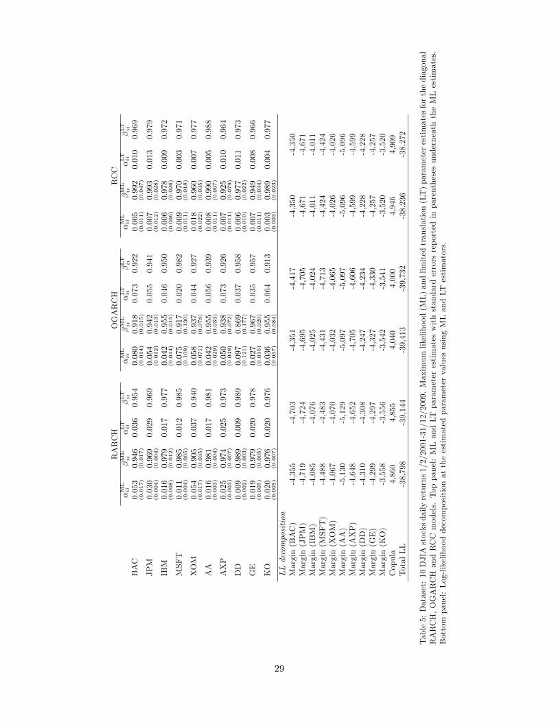
Table5:Dataset:10DJIAstocksdailyreturns1/2/2001-31/12/2009.Maximum
likelihood(ML)andlimitedtranslation(LT)parameterestimatesforthediagonal
RARCH,OGARCHandRCCmodels.Toppanel:MLandLT
parameterestimateswithstandarderrorsreportedinparenthesesunderneaththeMLestimates.
Bottompanel:Log-likelihooddecompositionattheestimatedparametervaluesusingMLandLT
estimators.
29

In Table 5 we analyze the results of the EB and LT estimators. As discussed in Section 3.2, the
EB estimator may result in strong shrinkage e¤ects, depending on the parameters�standard errors and
distance from the mean estimate, which may result in violations of the parameter restrictions required for
the diagonal model. In all three cases, we used the LT estimator to cushion against such e¤ects. In the
RARCH model, we set D = 1, while for the OGARCH and RCC models, we set D = 0:5; see (17). The
table reports the QML estimates along with their standard errors, and the LT estimates. The parameters
in the RARCH and OGARCH models are directly linked to the respective assets. In the case of RCC,
the parameters of BAC, for instance, are those which parameterize the correlation dynamics of BAC with
the remaining assets, and so on.
In the RARCH model, the e¤ect of shrinkage is strongest in the parameters of BAC and XOM. The
�MLii is quite high for these assets, implying less smoothness in the conditional variances and stronger-
than-average responsiveness to the shocks. Shrinkage leads to a notable deterioration in the �t of BAC�s
conditional variance, while XOM�s �t is almost una¤ected. Interestingly the copula �t is not drastically
a¤ected, and so the overall deterioration in the joint log-likelihood is mostly due to BAC�s marginal log-
likelihood. Testing the predictive ability of D-RARCH according to the QML estimates against the LT
estimates gives a t-statistic of 5.81 suggesting that shrinkage is not suitable in this case. This mirrors the
results in Table 4 where it is shown that moving from a diagonal to a scalar RARCH (implying shrinkage
to scalar parameters) leads to a statistically signi�cant reduction in predictive ability.
In the OGARCH case where there is higher heterogeneity among the dynamic parameters, noticeable
shrinkage is applied to almost half of the assets. Given the OGARCH model�s structure, this results in
a worse �t mostly in the margins while the copula log-likelihood only decreases marginally. Shrinkage
leads to a statistically signi�cant reduction in predictive ability with a t-statistic of 3.66. Again, this
mirrors the result when imposing common dynamic parameters as in the S-OGARCH model. In the case
of RCC, the �LTii estimates show considerable di¤erence compared to �MLii for many of the assets as they
are shrunk towards the mean estimate. These parameters control only the evolution of the conditional
correlations and so the �t of the margins is una¤ected. There is a slight deterioration in the copula �t
but it is not statistically signi�cant when using the predictive ability test. For the joint log-likelihood,
the predictive ability test for the unshrunk versus the shrunk model gives a t-statistic of -0.10 implying
that RCC dynamic parameters are not adversely a¤ected by shrinkage.
30

5 Conclusion
This paper advocates a rotation technique for raw returns which leads to easy-to-�t multivariate volatility
models via covariance targeting. We introduce the RARCH and RCC models to study the dynamics of the
conditional covariance matrix of daily asset returns, highlighting the similarities and di¤erences between
our approach and the class of OGARCH models.
We focus on diagonal structures and introduce the common persistence speci�cation as a more-tightly-
parameterized alternative to the diagonal speci�cation. Quasi-maximum likelihood estimation for our
model is computationally attractive, thanks to the convenient form of covariance targeting with a long-
run identity matrix. We also discuss the use of empirical Bayes methods for estimation, which provides
additional insight into the poolability of the dynamic parameters.
Empirical analysis shows that our model leads to statistically signi�cant gains in the 1-step predic-
tive joint likelihood compared to OGARCH and GOGARCH, and that capturing the dynamics of the
covariances of the rotated returns does improve the prediction of the conditional correlations. Given its
�exibility, the RCC model performs best in the 10-dimensional case we study, and our proposed common
persistence speci�cation performs quite favourably in comparison to the diagonal speci�cation.
Acknowledgements
We would like to thank Monica Billio, Tim Bollerslev, Christian Hafner and seminar participants at the
Oxford-Man Institute internal seminar series for helpful comments and suggestions.
References
Aielli, G. P. (2006). Consistent estimation of large scale dynamic conditional correlations. Unpublished paper:Department of Statistics, University of Florence.
Alexander, C. (2001). Orthogonal GARCH. In Mastering Risk, Volume 2, pp. 21�38. Prentice Hall.
Alexander, C. O. and A. M. Chibumba (1997). Multivariate orthogonal factor GARCH. Mimeo: University ofSussex, UK.
Amisano, G. and R. Giacomini (2007). Comparing density forecasts via weighted likelihood ratio tests. Journal ofBusiness & Economic Statistics 25, 177�190.
Bauwens, L., C. M. Hafner, and D. Pierret (2011). Multivariate volatility modelling of electricity futures. Journalof Applied Econometrics. Forthcoming.
Bauwens, L., S. Laurent, and J. V. K. Rombouts (2006). Multivariate GARCH models: a survey. Journal of AppliedEconometrics 21, 79�109.
Billio, M. and M. Caporin (2009). A generalized dynamic conditional correlation model for portfolio risk evaluation.Mathematics and Computers in Simulation 79, 2566�2578.
31

Billio, M., M. Caporin, and M. Gobbo (2006). Flexible dynamic conditional correlation multivariate GARCHmodels for asset allocation. Applied Financial Economics Letters 2, 123�130.
Boswijk, H. P. and R. van der Weide (2011). Method of moments estimation of GO-GARCH models. Journal ofEconometrics. Forthcoming.
Brownlees, C. T. (2010). On the relation between �rm characteristics and volatility dynamics with an applicationto the 2007-2009 �nancial crisis. Working paper: Stern School of Business, New York University.
Cappiello, L., R. F. Engle, and K. Sheppard (2006). Asymmetric dynamics in the correlations of global equity andbond returns. Journal of Financial Econometrics 4, 537�572.
Colacito, R., R. F. Engle, and E. Ghysels (2011). A component model for dynamic correlations. Journal ofEconometrics 164, 45�59.
Comte, F. and O. Lieberman (2003). Asymptotic theory for multivariate GARCH processes. Journal of MultivariateAnalysis 84, 61�84.
Cox, D. R. (1961). Tests of separate families of hypotheses. Proceedings of the Berkeley Symposium 4, 105�123.
Diebold, F. X. and R. S. Mariano (1995). Comparing predictive accuracy. Journal of Business & EconomicStatistics 13, 253�263.
Efron, B. (2010). Large-Scale Inference: Empirical Bayes Methods for Estimation, Testing and Prediction. Cam-bridge: Cambridge University Press.
Efron, B. and C. N. Morris (1972). Limiting the risk of Bayes and empirical Bayes estimators - part II. Journal ofthe American Statistical Association 67, 130�139.
Engle, R. F. (2002). Dynamic conditional correlation: a simple class of multivariate GARCH models. Journal ofBusiness and Economic Statistics 20, 339�350.
Engle, R. F. (2009a). Anticipating Correlations. Princeton University Press.
Engle, R. F. (2009b). High dimensional dynamic correlations. In J. L. Castle and N. Shephard (Eds.), TheMethodology and Practice of Econometrics: Papers in Honour of David F Hendry, pp. 122�148. Oxford UniversityPress.
Engle, R. F. and K. F. Kroner (1995). Multivariate simultaneous generalized ARCH. Econometric Theory 11,122�150.
Engle, R. F. and G. G. J. Lee (1999). A permanent and transitory component model of stock return volatility. InR. F. Engle and H. White (Eds.), Cointegration, Causality, and Forecasting. A Festschrift in Honour of CliveW.J. Granger, pp. 475�497. Oxford: Oxford University Press.
Engle, R. F. and J. Mezrich (1996). GARCH for groups. Risk 9, 36�40.
Engle, R. F., N. Shephard, and K. K. Sheppard (2008). Fitting vast dimensional time-varying covariance models.Unpublished paper: Oxford-Man Institute, University of Oxford.
Engle, R. F. and K. K. Sheppard (2001). Theoretical and empirical properties of dynamic conditional correlationmultivariate GARCH. Unpublished paper: UCSD.
Fan, J., M. Wang, and Q. Yao (2008). Modelling multivariate volatilities via conditionally uncorrelated components.Journal of the Royal Statistical Society, Series B 70, 679�702.
Francq, C. and J. M. Zakoian (2010). GARCH Models. Chichester: Wiley.
Giacomini, R. and H. White (2006). Tests of conditional predictive ability. Econometrica 74, 1545�1578.
32

Hafner, C. M. and P. H. Franses (2009). A generalized dynamic conditional correlation model: simulation andapplication to many assets. Econometric Reviews 28, 612�631.
James, W. and C. Stein (1961). Estimation with quadratic loss. In Proceedings of the Fourth Berkeley Symposiumin Math Statist. Prob, Volume 1, pp. 361�380. University of California.
Lanne, M. and P. Saikkonen (2007). A multivariate generalized orthogonal factor GARCH model. Journal ofBusiness and Economic Statistics 25, 61�75.
Morris, C. N. (1983). Parametric empirical Bayes inference: theory and applications. Journal of the AmericanStatistical Association 78, 47�55.
Newey, W. K. and D. McFadden (1994). Large sample estimation and hypothesis testing. In R. F. Engle andD. McFadden (Eds.), The Handbook of Econometrics, Volume 4, pp. 2111�2245. North-Holland.
Newey, W. K. and K. D. West (1987). A simple positive semi-de�nite, heteroskedasticity and autocorrelationconsistent covariance matrix. Econometrica 55, 703�708.
Noureldin, D., N. Shephard, and K. Sheppard (2011). Multivariate high-frequency-based volatility (HEAVY)models. Journal of Applied Econometrics. Forthcoming.
Pagan, A. (1986). Two stage and related estimators and their applications. Review of Economic Studies 53, 517�538.
Pakel, C., N. Shephard, and K. Sheppard (2011). Nuisance parameters, composite likelihoods and a panel ofGARCH models. Statistica Sinica 21, 307�329.
Ross, S. A. (1976). The arbitrage theory of capital asset pricing. Journal of Economic Theory 13, 341�360.
Silvennoinen, A. and T. Teräsvirta (2009). Multivariate GARCH models. In T. G. Andersen, R. A. Davis, J. P.Kreiss, and T. Mikosch (Eds.), Handbook of Financial Time Series, pp. 201�229. Springer-Verlag.
Song, P. X. K., Y. Fan, and J. D. Kalb�eisch (2005). Maximization by parts in likelihood inference. Journal of theAmerican Statistical Association 100, 1145�1169.
van der Weide, R. (2002). GO-GARCH: a multivariate generalized orthogonal GARCH model. Journal of AppliedEconometrics 17, 549�564.
Vuong, Q. H. (1989). Likelihood ratio tests for model selection and non-nested hypotheses. Econometrica 57,307�333.
A List of Stocks Used in Figure 1
The following is the list of stocks, with the ticker symbol in parentheses, from the S&P100 index used
in Figure 1: 3M Co. (MMM), AT&T Inc. (T), Abbott Laboratories (ABT), Alcoa (AA), Allstate Corp.
(ALL), Altria Group (MO), Amazon.com (AMZN), American Electric Power Co. (AEP), American
Express Inc. (AXP), Amgen Inc. (AMGN), Apple Inc. (AAPL), Avon Products Inc. (AVP), Baker
Hughes (BHI), Bank of America Corp. (BAC), Bank of New York (BK), Baxter International Inc.
(BAX), Boeing Co. (BA), Bristol-Myers Squibb (BMY), Burlington Northern Santa Fe Corp. (BNI),
CVS Caremark (CVS), Campbell Soup Co. (CPB), Capital One Financial Corp (COF), Chevron (CVX),
Caterpillar (CAT), Cisco Systems (CSCO), Citigroup Inc. (C), The Coca Cola Co. (KO), Colgate-
Palmolive Co. (CL), Comcast Corp. (CMCSA), ConocoPhillips (COP), Costco (COST), Dell (DELL),
33

Devon Energy (DVN), DuPont (DD), Dow Chemical (DOW), EMC Corp. (EMC), Entergy (ETR), Exelon
(EXC), Exxon Mobil Corp. (XOM), FedEx (FDX), Ford Motor (F), General Dynamics (GD), General
Electric (GE), Gilead Sciences (GILD), Goldman Sachs (GS), Halliburton (HAL), H. J. Heinz Co. (HNZ),
Hewlett Packard Co. (HPQ), Home Depot (HD), Honeywell International (HON), Intel Corp. (INTC),
International Business Machines (IBM), JP Morgan Chase & Co. (JPM), Johnson & Johnson Inc. (JNJ),
Lockheed Martin (LMT), Lowe�s Companies Inc. (LOW), McDonald�s Corp. (MCD), Medtronic Inc.
(MDT), Merck & Co. (MRK), Microsoft (MSFT), Morgan Stanley (MS), Nike (NKE), National Oilwell
Varco Inc. (NOV), Norfolk Southern Corp (NSC), Occidental Petroleum Corp. (OXY), Oracle Corp.
(ORCL), Pepsico Inc. (PEP), P�zer Inc. (PFE), Procter & Gamble Co. (PG), Qualcomm Inc. (QCOM),
Raytheon Co. (RTN), Regions Financial (RF), Sara Lee Corp. (SLE), Schering-Plough Corporation
(SGP), Schlumberger (SLB), Southern Co. (SO), Sprint Nextel Corp. (S), Target Corp. (TGT), Texas
Instruments (TXN), Time Warner Inc. (TWX), Tyco International (TYC), US Bancorp (USB), United
Parcel Service Inc. (UPS), United Technologies Corp. (UTX), UnitedHealth Group Inc. (UNH), Verizon
Communications Inc. (VZ), Wal-Mart Stores Inc. (WMT), Walgreen co. (WAG), The Walt Disney Co.
(DIS), Wells Fargo & Co. (WFC), Weyerhaeuser Co. (WY), Williams Companies (WMB), Wyeth (WYE)
and Xerox (XRX).
34