NeuroImage 62 (2012) 1848–1856

Contents lists available at SciVerse ScienceDirect

NeuroImage

j ourna l homepage: www.e lsev ie r .com/ locate /yn img

A multidimensional magnetic resonance histology atlas of the Wistar rat brain

G. Allan Johnson a,b,⁎, Evan Calabrese a,b, Alexandra Badea a, George Paxinos d,e, Charles Watson c,d,e

a Center for In Vivo Microscopy, Department of Radiology, Box 3302 Duke University Medical Center, Durham, NC 27710, USAb Biomedical Engineering, Box 90281 Duke University, Durham, NC 27708, USAc Health Sciences, Curtin University, Bentley, Western Australia, Australiad Neuroscience Research Australia, Australiae The University of New South Wales, Randwick, Australia

⁎ Corresponding author at: Center for In Vivo MicroscMedical Center, Durham, NC 27710, USA. Fax: +1 919

E-mail address: gjohnson@duke.edu (G.A. Johnson).

1053-8119/$ – see front matter © 2012 Elsevier Inc. Alldoi:10.1016/j.neuroimage.2012.05.041

a b s t r a c t

a r t i c l e i n f o

Article history:Accepted 18 May 2012Available online 24 May 2012

Keywords:Rat brainMRIAtlasDiffusion tensor imaging

We have produced a multidimensional atlas of the adult Wistar rat brain based on magnetic resonance his-tology (MRH). This MR atlas has been carefully aligned with the widely used Paxinos–Watson atlas basedon optical sections to allow comparisons between histochemical and immuno-marker data, and the use ofthe Paxinos–Watson abbreviation set. Our MR atlas attempts to make a seamless connection with the advan-tageous features of the Paxinos–Watson atlas, and to extend the utility of the data through the unique capa-bilities of MR histology: a) ability to view the brain in the skull with limited distortion from shrinkage orsectioning; b) isotropic spatial resolution, which permits sectioning along any arbitrary axis without loss ofdetail; c) three-dimensional (3D) images preserving spatial relationships; and d) widely varied contrast de-pendent on the unique properties of water protons. 3D diffusion tensor images (DTI) at what we believe to bethe highest resolution ever attained in the rat provide unique insight into white matter structures and con-nectivity. The 3D isotropic data allow registration of multiple data sets into a common reference space to pro-vide average atlases not possible with conventional histology. The resulting multidimensional atlas thatcombines Paxinos–Watson with multidimensional MRH images from multiple specimens provides a new,comprehensive view of the neuroanatomy of the rat and offers a collaborative platform for future rat brainstudies.

© 2012 Elsevier Inc. All rights reserved.

Introduction

The evolution of histological brain atlases has been marked by theprogressive introduction of new technologies, each of which has cre-ated new opportunities for more accurate mapping and greater un-derstanding. Until 1982, the most widely used atlases of the ratbrain were based on myelin-stained sections (König and Klippel,1963) or Nissl-stained coronal sections (Pellegrino et al., 1979), andnone offered a satisfactory stereotaxic system. The Paxinos andWatson (1982) rat brain atlas was the first to take advantage of histo-chemical staining, the first to offer a comprehensive and accurate ste-reotaxic system, and the first to picture labeled brain sections in allthree cardinal planes. This atlas also marked the introduction of anew abbreviation set, which has since become the most widely usedin the field of neuroscience, and has been adopted by almost allmajor mammalian and avian brain atlases (Ashwell and Paxinos,2008; Franklin and Paxinos, 2007; Mai et al., 2008; Morin andWood, 2001; Paxinos et al., 2007, 2009a, 2009b, 2010; Puelles et al.,2007; Watson and Paxinos, 2010).

opy, Box 3302 Duke University684 7158.

rights reserved.

Since its first release in 1982, the Paxinos andWatson (for simplic-ity “P–W”) atlas has gone through rapid evolution, culminating in the6th edition in 2007 (Paxinos and Watson, 1982, 1986, 1997, 1998,2005, 2007). The new features include the use of a wide range of im-munohistochemical markers (Paxinos et al., 2009a, 2009b) and geneexpression patterns (www.alleninstitute.org), the delineation ofabout 1000 structures (versus 400 in the 1st edition), and thedevelopment of a web-based version featuring 3D reconstructions(BrainNavigator www.brainnav.com). In addition, the comprehensivenomenclature set has been structured in the form of an ontologybased on developmental gene expression patterns (available onBrainNavigator).

Conventional histological atlases of the rat brain will continue toevolve. This article describes the addition of magnetic resonance his-tology (MRH) data, accompanied by a range of new benefits to theuser. The evolution of atlases does not mean the replacement of theold by the new, but the continuing emergence of new types thattake advantage of new technologies. The new types adopt the impor-tant features that developed in earlier atlases. A modern MRH atlasshould incorporate all of the best features of the conventional histo-logical atlases, while offering new technological advantages to users.

Johnson et al. introduced the first magnetic resonance imaging(MRI) atlas of the live rat in 1987 (Johnson et al., 1987). The

1849G.A. Johnson et al. / NeuroImage 62 (2012) 1848–1856

realization in 1993 that MRI could be used to study the structure offixed tissue introduced the concept of magnetic resonance histology(MRH) (Johnson et al., 1993). Over the last 25 years, MR atlaseshave evolved with higher spatial resolution, 3D acquisitions with iso-tropic voxels (Suddarth and Johnson, 1991), and an increasingly richset of contrast mechanisms. Table 1 summarizes some of this work forthe rat. The table covers a literature search using the terms “MRI,”“atlas,” and “rat” over the last 25 years. Magnetic field strength rangesfrom 1.5 T to 9.4 T. A number of sequences have been used, which em-phasize different contrasts in the tissue (column 4): T1—emphasizingdifference in spin lattice relaxation time; T2—emphasizing differencein spin relaxation time; PD—based on differences in proton density;and diffusion tensor images (DTI)—providing a suite of contrast param-eters based on tissue-specific diffusion of water. Both two-dimensional(2D) and three-dimensional (3D) imaging sequences have been used.To allow comparisons of resolution between two sequences, we includethe slice thickness and in-plane resolution. The product of slice andin-plane resolution yields the voxel volume (column 7), which is themost appropriate comparison of resolution. By normalizing this voxelvolume to the voxel volume in this work (15.6×10−6 mm3), one isable to readily compare the differences in resolutions. For example,the first rat MRI atlas in 1987 was based on contiguous slices thatwere 1.2-mm thick within in-plane resolution of 0.115 mm. The atlasshown here with 25-micron slices represents an increase in resolutionalong the z axis of 50 times. But the voxels of this first atlas(0.115×0.115×1.2 mm=15.9 nl) are 1025-times larger than thevoxels of this new atlas (0.025×0.025×0.025 mm=15.6 pl).

The majority of these rat atlases have been based on 2D multisliceimaging strategies (Cross et al., 2004; Johnson et al., 1987; Nie et al.,2010; Ramu et al., 2006; Schwarz et al., 2006; Schweinhardt et al.,2003; Ting and Bendel, 1992). The resolution is limited in 2D se-quences because of hardware capabilities and reduced signal relativeto 3D sequences. The introduction of 3D sequences with large arrays(Suddarth and Johnson, 1991), the use of active staining to reduceT1 (and allow shorter acquisitions) (Johnson et al., 2002), and the de-velopment of extended dynamic range (Johnson et al., 2007) havebeen crucial technical milestones required for isotropic imaging.While a number of mouse atlases have exploited these methods forisotropic imaging (Benveniste et al., 2000; Chen et al., 2006; Jiangand Johnson, 2011; Ma et al., 2005) the arrays have been much small-er. The 800×800×1600 arrays used here represent an increase indata volume of more than 30-times that of the mouse atlases. 3Ddata allows the development of a whole new class of atlases basedon population averages (Aggarwal et al., 2011; Bai et al., 2012;Chuang et al., 2011; Valdés-Hernández et al., 2011). Isotropic resolu-tion allows one to align images sets from multiple specimens regard-less of misalignments between specimens during scanning. The MRdata are acquired in the skull, so there is no damage to the brain

Table 1Comparison of MR atlases.

Year Reference Field(T)

Contrast

1987 (Johnson et al., 1987) 1.5 T11992 (Ting and Bendel, 1992) 4.7 T1, T2, PD2003 (Leergaard et al., 2003) 3.0 T12003 (Schweinhardt et al., 2003) 4.7 T1, T22004 (Cross et al., 2004) 1.5 T12006 (Ramu et al., 2006) 7.0 T22006 (Schwarz et al., 2006) 4.7 T22007 (Hjornevik et al., 2007) 3.0 T12010 (Nie et al., 2010) 7.0 T22010 (Lu et al., 2010) 9.4 T22011 (Veraart et al., 2011) 7.0 T1, DTI2012 This work 7.0 T2*, DTI

a The resolution is normalized to this work by dividing the encoding voxel volume by 0.

from extraction. The specimen preparation has been undertaken tominimize shrinkage and there is no distortion from physical sectioning.

As conventional histology atlases have evolved with variedchemical stains to highlight the chemoarchitecture, so too havethe MRH atlases evolved with different MRI contrasts. Sophisticat-ed image-processing methods developed for comparison of clini-cal images have been adapted to register multiple data sets intoaverage atlases with enhanced signal-to-noise and contrast-to-noise.

We present here what we believe to be the highest-resolution multidimensional MR atlas of the rat brain, withthe widest range of contrast mechanisms, including averageatlases with a total of 8 different types of contrast. The datahave been registered to the orientation defined by the Paxinosand Watson atlas, and provides a comprehensive new view ofthe adult Wistar rat.

Methods

Experimental animals

All experiments and procedures were done with the approval of theDuke University Institutional Animal Care and Use Committee. Fivepostnatal-day 80, male Wistar rats (Charles River Laboratories,Wilmington, MA, USA) weighing approximately 250 g were selectedfor imaging studies. Animals were perfusion fixed using the activestaining technique (Johnson et al., 2002) to introduce the gadolinium-based MRI contrast agent Gadoteridol (ProHance, Bracco DiagnosticsInc., Princeton, NJ, USA) into the brain parenchyma. After flushing thevasculature with normal saline, perfusion fixation was achieved usinga 10% solution of neutral buffered formalin (NBF) containing 10%(50 mM) gadoteridol. After perfusion fixation, rat heads were removedfrom the torso and immersed in 10% NBF for 24 h. Finally, fixed ratheads (i.e., with brains still in the cranium) were transferred to a 0.1 Msolution of phosphate buffered saline containing 1% (5mM) gadoteridolat 4°C for 5–7 days to ensure equilibration of contrast agent, and tissuerehydration. This final step of rehydration in normal buffered salineminimizes any shrinkage or swelling. The active staining technique re-duces the T1 relaxation time of the brain parenchyma to less than100 ms and allows faster, higher-resolution imaging with highersignal-to-noise ratio (SNR) (Johnson et al., 2002). Prior to imaging, spec-imens were placed in custom-made, MRI-compatible tubes andimmersed in a liquid fluorocarbon (Fomblin perfluoropolyether,Ausimont, Thorofare, NJ, USA) to reduce susceptibility artifacts at tissueinterfaces and to prevent specimen dehydration. All imaging experi-ments were performed with the brain in the cranium to preserve itsnatural shape.

Slice(mm)

In plane(Mm)

Voxel(mm3)

Relativea

1.2 0.115×0.115 0.016 10250.6 0.175×175 0.018 11770.39 0.390×0.390 0.059 37820.5 0.117×0.117 0.007 4480.5 0.273×250 0.034 21791.0 0.137×0.137 0.019 12031.0 0.156×0.156 0.024 15380.195 0.195×0.195 0.007 4490.3 0.14×0.14 0.00588 3771.0 0.137×0.137 0.0187 11990.088 0.088×0.088 0.00068 440.025 0.025×0.025 0.0000156 1

0000156, i.e. the volume of the voxels in our gradient recalled echo (GRE) image.

1850 G.A. Johnson et al. / NeuroImage 62 (2012) 1848–1856

Data acquisition

Images were acquired on a 7 T small animal MRI system (MagnexScientific, Yarnton, Oxford, UK) equipped with 750 mT/m ResonanceResearch gradient coils (Resonance Research, Inc., Billerica, MA,USA), and controlled with a General Electric Signa console (GE Med-ical Systems, Milwaukee, WI, USA). RF excitation and receptionwere accomplished using a custom-made 30-mm diameter×50-mmlong solenoid RF coil. T2*-weighted structural images were acquiredusing a 3D gradient recalled echo (GRE) sequence (flip angleα=60°, TR=50 ms, TE=8.3 ms, NEX=2) with a strategy designedto provide the wide dynamic range required for large 3D arrays, de-scribed more completely in Johnson et al. (2007). The data werefully sampled in Fourier space with an acquisition matrix of 1600(frequency)×800 (phase)×800 (phase) over a 40×20×20 mmfield of view (FOV), yielding Nyquist limited isotropic voxel size of25 μm3 (voxel volume=15.6 pl). Data presented here have notbeen interpolated by zero filling. Approximate scan time was 13 hper specimen.

Diffusion-weighted images were acquired using an RF refocusedspin-echo pulse sequence (TR=100 ms, TE=16.5 ms, NEX=1).The acquisition matrix was 800×400×400 over a 40×20×20 mmFOV for a Nyquist-limited isotropic voxel of 50 μm3 (voxel vol-ume=125 pl). Diffusion preparation was accomplished using a mod-ified Tanner–Stejskal diffusion-encoding scheme with a pair ofunipolar, half-sine diffusion gradient waveforms (width [δ]=3 ms,separation [Δ]=8.5 ms, gradient amplitude=600 mT/m). One base-line image with b=0 (b0) and 6 high b-value images (b=1462 s/mm2) were acquired with diffusion sensitization along each of 6non-collinear diffusion gradient vectors' directions [1, 1, 0], [1, 0, 1],[0, 1, 1], [−1, 1, 0], [1, 0, −1], and [0, −1, 1]. Total acquisition timewas approximately 38 h.

Diffusion tensor image processing pipeline

Diffusion-weighted image processing was carried out using an au-tomated DTI processing pipeline written in Perl (www.perl.org), andMATLAB (MathWorks, Natick, MA). After image reconstruction, alldiffusion-weighted images were registered to the b0 image usingAdvanced Normalization Tools (ANTs) (Avants et al., 2008) using a6-parameter rigid affine registration to correct for the linear compo-nent of eddy current distortions. For each specimen (n=5), wederived 6 different DTI data sets. For each specimen, the b0 imageand the 6 DWI images were then combined into a single 4D volumeto simplify processing. Diffusion Toolkit (www.trackvis.org/dtk) com-mand line tools were used to calculate the diffusion tensor, the 3 ei-genvalues and 3 eigenvectors, and 6 tensor-derived image sets—anapparent diffusion coefficient map (ADC), an isotropic diffusion-weighted image (DWI), a longitudinal diffusivity map (LD), a radialdiffusivity map (RD), a fractional anisotropy (FA) map, and adirectionally-encoded FA color-map. Automated skull stripping ofthe DWI was performed using a modified version of the skull-stripping algorithm described in Badea et al. (2007), and the maskwas propagated to all other co-registered image sets. Finally, themask was used as a region of interest for whole-brain fibertractography using the Diffusion Toolkit implementation of the FACTalgorithm (Mori et al., 1999) with fractional anisotropy thresh-old=0.25 and angle threshold=45°. All tractography data were vi-sualized and analyzed using TrackVis interactive visualizationenvironment (www.trackvis.org).

Image registration and population averaging

Inter-specimen registration of the all the MR data was accom-plished with the ANTs software package using an iterative registra-tion strategy similar to that described in Johnson et al. (2010).

Skull-stripped FA and gradient recalled echo (GRE) images fromeach of the 5 specimens were aligned using a 12-parameter affineregistration, followed by an iterative diffeomorphic deformable regis-tration process designed to maximize cross-correlation. Data registra-tion was achieved using a Minimum Deformation Template (MDT)strategy, which uses a viscous fluid deformation model for dif-feomorphic registration (Avants et al., 2008). The MDT strategy usespairwise, non-linear image registrations to construct an average tem-plate requiring the minimum amount of deformation from each of thestarting points (Kochunov et al., 2001). This technique is ideal foratlas construction because it creates an average data set with a mini-mum amount of individual bias. In short, the MDT is generated byperforming an iterative non-linear registration between each pair ofdata sets (for example, 5 data sets=10 possible pairs), producing adeformation field for each pair of data sets. All deformation fieldsfor a given data set are averaged to create a single, average deforma-tion field, which is then applied to the corresponding data set totransform it into the MDT space. The transformed data can then beaveraged to create a single average MDT data set. For more detailsabout this technique, see Veraart et al. (2011). The similarity metricwas cross-correlation (CC) with a weight of 1 (i.e. only this metricdrives registration), computed for a kernel radius of 4 voxels. Weused a multi-resolution scheme, and did a maximum of 4000 itera-tions at a downsampling factor of 3, 4000 iterations at a down-sampling factor of 2, and 200 iterations at full resolution. We usedthe greedy symmetric normalization (SyN) model with a gradientstep of 0.5 and a Gaussian regularization with a sigma of 3 for the sim-ilarity gradient, and a sigma of 1 for the deformation field.

One of the unique aspects of this collection of data is that for eachspecimen (n=5), we have acquired multiple images with contrastdifferentiation based on different physical phenomena. Since thespecimen remains in place during these multiple scans, all of thedata for a single specimen are co-registered so a single set of transfor-mations can be applied to each of the different image contrasts (all ofthe DTI data sets are registered to a common space during process-ing). The resulting affine and diffeomorphic transformations were ap-plied directly to the GRE images to generate a single population-averaged image volume. Transformations were applied to the tensorvolumes using log-Euclidean methods (i.e., the transforms were ap-plied to the matrix logarithm of the diagonalized tensor) because di-rect transformation of tensor volumes can result in null or negativeeigenvalues (Arsigny et al, 2006). We report here the following pop-ulation averages: gradient recalled echo (GRE), proton density (PD)based on the b=0 spin echo of the DTI acquisition, diffusion weight-ed image (DWI), apparent diffusion coefficient (ADC), longitudinaldiffusivity (LD), radial diffusivity (RD), fractional anisotropy (FA),and color-encoded fractional anisotropy (colorFA). In addition, an av-erage diffusion tensor image has been generated for tractography.Representative data are available from our web site (www.civm.duhs.duke.edu/neuro2012ratatlas).

Orientation of MR data to Paxinos–Watson

The slice thickness and the sampling interval in the MR data are25 μm for the GRE images. The slice thickness in P–W is 40 μm, butthe sampling interval for the horizontal sections is 220 μm. Sincethe MRH volume is an isotropic 3D array, one can resample planesat arbitrary angles with only limited degradation in spatial resolutionarising from interpolation. We have not attempted to “align” the MRand histology using the mathematical approaches used to align theindividual MR data sets to each other, since there is shrinkage anddistortion in the conventional sectioning. We have instead, tried toalign the axes of the MR data to the axes of the P–W atlas. This align-ment was a three-step process. We first oriented the coronal plane ofthe GRE image so the mid-sagittal plane is vertical and the left andright sides appear symmetrical in a coronal section. We then chose

1851G.A. Johnson et al. / NeuroImage 62 (2012) 1848–1856

three horizontal sections from the P–W atlas, which had anatomicallandmarks that are apparent in two (but not all three) of the P–Wsections shown in Fig. 1: the medial cerebellar nucleus (MedDL);the ventralmost aspect of the genu of the corpus callosum (gcc); theventralmost aspect of the posterior commissure (pc). Through an it-erative process, we were able to define reliable landmarks in fivehorizontal (dorsoventral) planes of the GRE image that are approxi-mately 1 mm apart. The angle of the horizontal plane used to reslicethe GRE images was adjusted until these landmarks (in the GRE im-ages) matched those in the three adjacent slices of Paxinos–Watson.

Results

Validation of the selected horizontal reference plane by examination oflandmarks in coronal sections

To ensure that the MR data sets were oriented as closely as possi-ble to that of the P–Watlas, we identified landmarks in a series of cor-onal slices and compared their rostrocaudal position with the same

Fig. 1. Three adjacent horizontal slices from the Paxinos andWatson atlas and the corresponbeen inverted to better match histology contrast. Row (a) corresponds to Paxinos and W(MedDL) is visible posteriorly, but the crossing of the posterior commissure (pc) and theto Paxinos and Watson Figure 199 (interaural 4.90 mm), the section immediately dorsal to Raspect of the gcc, the ventralmost aspect of the pc, and the dorsalmost aspect of MedDL. Romediately dorsal to Row (b). In this horizontal plane, MedDL is no longer visible, while the gseen in the histology sections.

structures pictured in the P–W atlas. The comparisons are shown inTable 2. The mean discrepancy in 21 comparisons was 0.27 mm,which is within the range of discrepancy that exists when landmarksin the P–W atlas were compared in different planes (Paxinos andWatson, 2007).

The alignment of the MRH and P–W atlas can be most easily ap-preciated in Fig. 2 in which the labels from the P–W atlas (Figure71, Bregma −4.56 mm) have been drawn on a coronal section fromthe GRE images after alignment with the P–W atlas. More than 60structures can be seen in the GRE images corresponding to delinea-tions in the P–W atlas

Features of the average multidimensional atlas

Since the MRH atlas from each specimen is three-dimensionalwith minimal distortion, it is possible to align multiple data setsusing the registration algorithms that have been developed for clini-cal MRI. The advantages can be seen in Fig. 3 in which a slice from asingle GRE image (Fig. 3a) is compared to the same slice in the

ding GRE images demonstrating the alignment of MR data to histology. MR contrast hasatson atlas Figure 198 (interaural 4.68). In this plane, the medial cerebellar nucleusgenu of the corpus callosum (gcc) are not yet visible anteriorly. Row (b) correspondsow (a). The three major landmarks that define this horizontal slice are the ventralmostw (c) corresponds to Paxinos and Watson Figure 200 (interaural 5.26), the section im-cc and pc remain in plane. The corresponding MR images closely match the landmarks

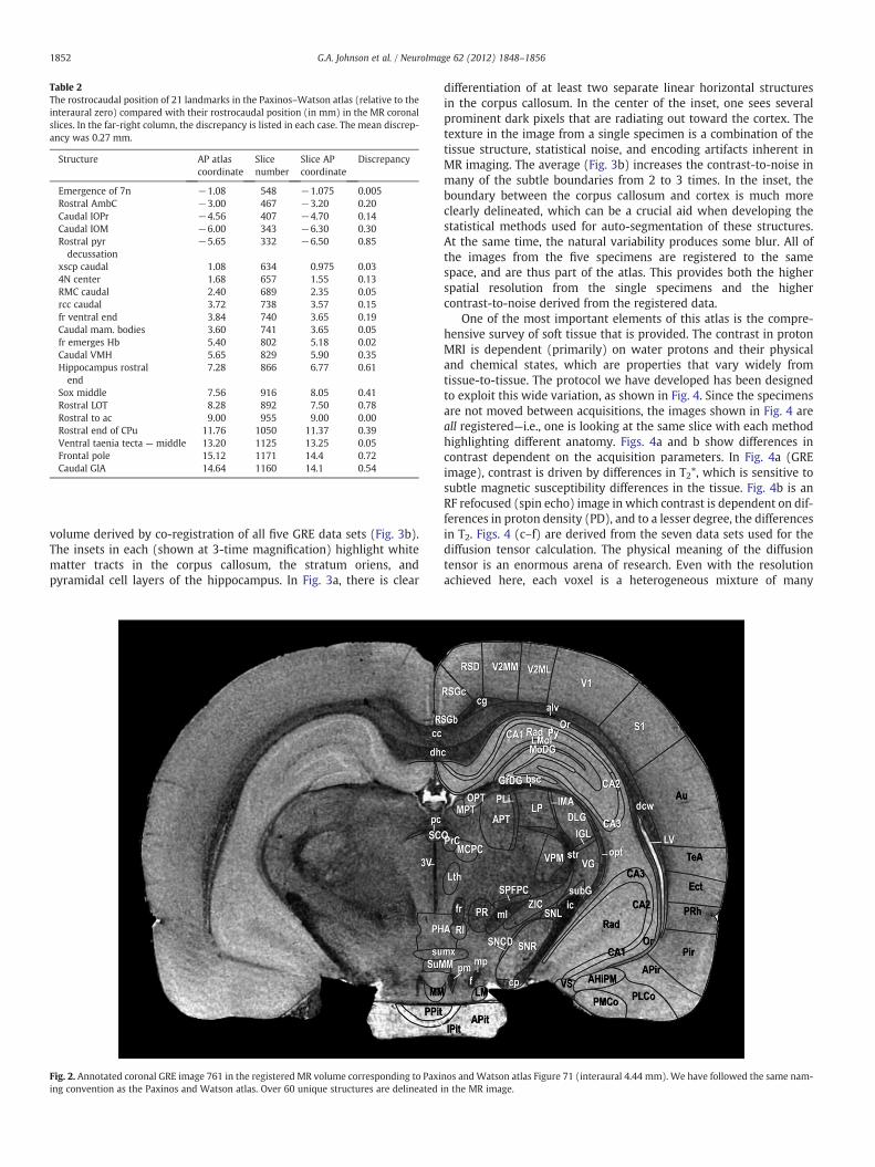
Table 2The rostrocaudal position of 21 landmarks in the Paxinos–Watson atlas (relative to theinteraural zero) compared with their rostrocaudal position (in mm) in the MR coronalslices. In the far-right column, the discrepancy is listed in each case. The mean discrep-ancy was 0.27 mm.

Structure AP atlascoordinate

Slicenumber

Slice APcoordinate

Discrepancy

Emergence of 7n −1.08 548 −1.075 0.005Rostral AmbC −3.00 467 −3.20 0.20Caudal IOPr −4.56 407 −4.70 0.14Caudal IOM −6.00 343 −6.30 0.30Rostral pyrdecussation

−5.65 332 −6.50 0.85

xscp caudal 1.08 634 0.975 0.034N center 1.68 657 1.55 0.13RMC caudal 2.40 689 2.35 0.05rcc caudal 3.72 738 3.57 0.15fr ventral end 3.84 740 3.65 0.19Caudal mam. bodies 3.60 741 3.65 0.05fr emerges Hb 5.40 802 5.18 0.02Caudal VMH 5.65 829 5.90 0.35Hippocampus rostralend

7.28 866 6.77 0.61

Sox middle 7.56 916 8.05 0.41Rostral LOT 8.28 892 7.50 0.78Rostral to ac 9.00 955 9.00 0.00Rostral end of CPu 11.76 1050 11.37 0.39Ventral taenia tecta — middle 13.20 1125 13.25 0.05Frontal pole 15.12 1171 14.4 0.72Caudal GlA 14.64 1160 14.1 0.54

1852 G.A. Johnson et al. / NeuroImage 62 (2012) 1848–1856

volume derived by co-registration of all five GRE data sets (Fig. 3b).The insets in each (shown at 3-time magnification) highlight whitematter tracts in the corpus callosum, the stratum oriens, andpyramidal cell layers of the hippocampus. In Fig. 3a, there is clear

Fig. 2. Annotated coronal GRE image 761 in the registered MR volume corresponding to Paxiing convention as the Paxinos and Watson atlas. Over 60 unique structures are delineated

differentiation of at least two separate linear horizontal structuresin the corpus callosum. In the center of the inset, one sees severalprominent dark pixels that are radiating out toward the cortex. Thetexture in the image from a single specimen is a combination of thetissue structure, statistical noise, and encoding artifacts inherent inMR imaging. The average (Fig. 3b) increases the contrast-to-noise inmany of the subtle boundaries from 2 to 3 times. In the inset, theboundary between the corpus callosum and cortex is much moreclearly delineated, which can be a crucial aid when developing thestatistical methods used for auto-segmentation of these structures.At the same time, the natural variability produces some blur. All ofthe images from the five specimens are registered to the samespace, and are thus part of the atlas. This provides both the higherspatial resolution from the single specimens and the highercontrast-to-noise derived from the registered data.

One of the most important elements of this atlas is the compre-hensive survey of soft tissue that is provided. The contrast in protonMRI is dependent (primarily) on water protons and their physicaland chemical states, which are properties that vary widely fromtissue-to-tissue. The protocol we have developed has been designedto exploit this wide variation, as shown in Fig. 4. Since the specimensare not moved between acquisitions, the images shown in Fig. 4 areall registered—i.e., one is looking at the same slice with each methodhighlighting different anatomy. Figs. 4a and b show differences incontrast dependent on the acquisition parameters. In Fig. 4a (GREimage), contrast is driven by differences in T2*, which is sensitive tosubtle magnetic susceptibility differences in the tissue. Fig. 4b is anRF refocused (spin echo) image in which contrast is dependent on dif-ferences in proton density (PD), and to a lesser degree, the differencesin T2. Figs. 4 (c–f) are derived from the seven data sets used for thediffusion tensor calculation. The physical meaning of the diffusiontensor is an enormous arena of research. Even with the resolutionachieved here, each voxel is a heterogeneous mixture of many

nos andWatson atlas Figure 71 (interaural 4.44 mm). We have followed the same nam-in the MR image.

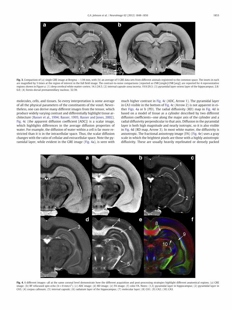
Fig. 3. Comparison of (a) single GRE image at Bregma −1.94 mm, with (b) an average of 5 GRE data sets from different animals registered to the common space. The insets in eachare magnified by 3 times at the region of interest in the full field image. The contrast-to-noise comparisons (reported as CNR [single]/CNR [avg]) are reported for 4 representativeregions shown in Figure a: (1) deep cerebral white matter-cortex; 14.1/24.5; (2) internal capsule-zona incerta; 19.9/29.3; (3) pyramidal layer-oriens layer of the hippocampus; 2.8/6.0; (4) fornix-dorsal premammillary nucleus; 32/39.

1853G.A. Johnson et al. / NeuroImage 62 (2012) 1848–1856

molecules, cells, and tissues. So every interpretation is some averageof all the physical parameters of the constituents of the voxel. Never-theless, one can derive many different images from the tensor, whichproduce widely varying contrast and differentially highlight tissue ar-chitecture (Basser et al., 1994; Basser, 1995; Basser and Jones, 2002).Fig. 4c (the apparent diffusion coefficient [ADC]) is a scalar image,which highlights differences in the average diffusion properties ofwater. For example, the diffusion of water within a cell is far more re-stricted than it is in the intracellular space. Thus, the scalar diffusionchanges with the ratio of cellular and extracellular space. Note the py-ramidal layer, while evident in the GRE image (Fig. 4a), is seen with

Fig. 4. 6 different images—all at the same coronal level demonstrate how the different acqimage; (b) RF refocused spin echo (b=0 mm/s2); (c) ADC image; (d) RD image; (e) FA imCA3; (4) corpus callosum; (5) internal capsule; (6) radiatum layer of the hippocampus; (7

much higher contrast in Fig. 4c (ADC, Arrow 1). The pyramidal layerin CA3 visible in the bottom of Fig. 4c (Arrow 2) is not apparent in ei-ther Figs. 4a or b (PD). The radial diffusivity (RD) map in Fig. 4d isbased on a model of tissue as a cylinder described by two differentdiffusion coefficients—one along the major axis of the cylinder and aradial diffusivity perpendicular to that axis. Diffusion in the pyramidallayer is both high magnitude and nearly isotropic, so it is also visiblein Fig. 4d (RD map, Arrow 3). In most white matter, the diffusivity isanisotropic. The fractional anisotropy image (FA) (Fig. 4e) uses a grayscale in which the brightest pixels are those with a highly anisotropicdiffusivity. These are usually heavily myelinated or densely packed

uisition and post-processing strategies highlight different anatomical regions. (a) GREage; (f) color FA. Notes: (1,3) pyramidal layer in hippocampus; (2) pyramidal layer in) molecular layer; (8) CA1; (9) CA2; (10) CA3.

Fig. 6. DTI data can be used to extract fiber connectivity between regions. (a)Tractography volume of the whole brain showing 3% of the fibers detected. (b) Fibertracts in specific structures (e.g., the anterior commissure) can be isolated. (c) Magni-fied view of the tractography data in the anterior commissure demonstrates the exqui-site spatial resolution of these data.

Fig. 5. A volume-rendered image helps define three-dimensional relationships that aresometimes difficult to appreciate in planar images. 20 different sub-volumes of thebrain have been delineated with the boundaries between volumes defined by the con-trast in all of the data. Nine of those sub-volumes are volume-rendered here.

1854 G.A. Johnson et al. / NeuroImage 62 (2012) 1848–1856

and coherently organized axons. Note the bright corpus callosum(Arrow 4) and internal capsule (Arrow 5). However, the FA can alsohighlight other structures that are not white matter if the underlyingcytoarchitecture directionally alters the diffusion of water. For exam-ple, note the radiatum layer (Arrow 6) and molecular layers of thedentate gyrus (Arrow 7) in the hippocampus. Both of these layershave significant numbers of axons radiating outward so the anisotro-py, while not as high as heavily myelinated white matter, is still suf-ficient to provide some differential contrast. The directionallyencoded FA color map (Fig. 4f) encodes both the degree of anisotropy(intensity) and direction (hue). Voxels in which the greatest diffusiv-ity is anterior–posterior are encoded in blue and voxels in which thediffusivity is greatest along the dorsal–ventral axis are in green, withthe remaining lateral dimension encoded in red. The corpus callosum(red) and cingulum (green), both bright in the FA image, are nowclearly differentiated, based on the direction of the fiber tracts. Inareas where the anisotropy is less dramatic, the color can still help de-fine the anatomy. Note now in the radiatum layer and molecular layerof the dentate gyrus in the hippocampus, one can distinguish subtleshading differences between CA1 (Arrow 8), CA2 (Arrow 9), andCA3 (Arrow 10) related to the direction of the radiating axons. Sever-al good reviews of the underlying physics of DTI and the conventionsfor display include Basser and Jones (2002) and Mukherjee et al.(2008).

Finally, all of the data in this atlas are three-dimensional. In Fig. 5,a collection of 9 different structures has been rendered to appreciaterelationships that might be more difficult to understand in planarslices. As noted previously, the boundaries of some structures aremore apparent in the ADC image, while others are more apparent inthe FA image. Structure delineation can be done with all the variedcontrast sets and transferred into a single comprehensive label setthat can be resliced along any plane and rendered from any angle.

Fig. 6 extends the dimensionality of the data yet again with avolume-rendered image of white matter tracts derived from theDTI. Using freely available tools (such as TrackVis www.trackvis.org), one can select any region of interest and display only tractsthat pass through it. In Fig. 6a, we have selected an FA threshold of0.25 to render fiber tracts. Because the signal-to-noise and resolutionare both high, this results in a considerable number of tracts. To facil-itate display, only 3% of the detected tracts are shown in Fig. 6a. Amid-sagittal section from the GRE image (downsampled to matchthe DTI) is included for reference. In Fig. 6b, we have limited the dis-play to 3% of the tracts in the anterior commissure. Again, the mid-sagittal GRE image provides context. The magnified image (Fig. 6c)

allows one to appreciate the spatial resolution that is unique to thisdata. Even at this resolution, the single-tensor tractography model islimited by the fact that the dimensions of the voxels are significantlylarger than the individual neuronal tracts. But, the resolution in thesedata is the highest yet published, which serves to reduce the ambigu-ity from crossing fibers.

Discussion

This is not the first MR atlas of the rat brain andmost probably willnot be the last. Atlases continue to evolve as new stains develop fortraditional histology and new technology evolves for digital imagingmethods. The important features of this new atlas are as follows:

1. We have provided the highest-resolution MRI data yet attained. AsTable 1 demonstrates, the resolution of the gradient recalled im-ages is nearly 44-times higher than that of our previous workwith the Sprague Dawley rat, and more than 400-times higherthan that of any other MR atlases.

2. We have registered the data to the historical reference space de-fined by Paxinos and Watson that has long served as the definitiveneuroanatomic reference for the Wistar rat. This alignment facili-tates direct comparison between the chemoarchitectonic atlasesand this new modality, and allows translation of the well-

1855G.A. Johnson et al. / NeuroImage 62 (2012) 1848–1856

established nomenclature from previous work into this new di-mension of the atlas.

3. We have provided images with a comprehensive range of MR con-trast mechanisms enabling, for example, the delineation of verysmall structures (granular layer in the hippocampus) with gradi-ent recalled images and subtle contrast (e.g., subthalamic nucleiusing the ADC). The data for each individual specimen are all reg-istered so one can simultaneously view the same cytoarchitecturewith multiple MRI contrasts. Structures not seen with one contrastcan be readily appreciated with an alternate contrast mechanism,with minimal registration errors.

4. We have provided data sets from five different specimens acquiredwith our comprehensive protocol. The protocol provides the mostrobust registration yet the large data arrays are isotropic, allowinginteractive simultaneous display of multiple planes along any arbi-trary axis without loss of spatial resolution. Some anatomic con-nections not readily appreciated in a single cardinal planebecome more apparent. Quantitative morphometric measures arevastly improved over measures done on conventional histologysince the image data are isotropic, from a brain in the skull, andwith fully hydrated tissue that has undergone minimal shrinkageor tissue damage during extraction from the skull. We have includ-ed a data set for the supplemental web site (http://www.civm.duhs.duke.edu/neuro2012ratatlas) (prior to skull stripping) thatdemonstrates the limited change in tissue volume by noting thespace between the dura of the brain and the skull. The majorityof previous rat atlases have used 2D sequences with thick slices.Isotropic 3D imaging has been used for several mouse atlases.But, the majority of these atlases use relatively small image arrays(256×256×512). The unique technical approach used in thiswork allowed us to acquire image arrays that are more than 30-times that of the majority of the mouse atlases. The combinationof multiple 3D images with very large arrays at the highest spatialresolution from multiple specimens with DTI data allows one toperform comparative studies not possible with any previousmethod.

These data are an extension of previous work in the mouse(Waxholm Space) (Johnson et al., 2010; Jiang and Johnson, 2011) thatwas undertaken to facilitate comparisons and collaborations acrosslaboratories. One of the major shortcomings of that work was the factthat the original orientation was not undertaken with concern for con-nection to existing cytoarchitectonic atlases. As a consequence, thereare far fewer structures labeled in the mouse data. Since those mousedata are isotropic like the rat data discussed here, it is relatively straight-forward to perform the necessary transformations. This work is nowunder way to connectWaxholm Space to that of the existing traditionalatlases. The careful initial registration of all these rat data to thePaxinos–Watson atlas should make this atlas muchmore readily acces-sible to the neuroscience community.

Like Waxholm Space, these data provide a framework to facilitatecollaboration in neuroscience (see International NeuroinformaticsCoordinating Facility [www.incf.org]). Since the data are of high reso-lution, in three dimensions, with high signal-to-noise, and a widerange of contrasts, researchers should be able to register their datato these. Once done, any point in their work is immediately translatedto this 3D space and the Paxinos–Watson atlas, along with a commonnomenclature.

Conventional histologic procedures still provide the highest-resolution atlases for two-dimensional planar images. But, they arenot three-dimensional and they suffer significant distortion arisingfrom tissue processing. The resolution of this MRI data is sufficientlyhigh that traditional two-dimensional histology sections can be regis-tered to it. This provides the neuroscientist using these traditional ap-proaches a ready method for mapping their data into this commonspace.

Atlases are finding their way into many in vivo studies where ste-reotactic coordinates are useful. Since the range of contrast suppliedin our atlas is extensive, in vivo MRI studies done with nearly anytechnique can be readily registered using either single-channelmethods, or where necessary, more sophisticated multi-channelmethods. Lower-contrast studies, e.g., CT or lower-resolution studies(PET, SPECT) can be readily aligned using automated registrationalgorithms.

Structural delineations generated on this atlas can serve as thestarting point for segmentations from any of the image sources previ-ously mentioned. For example, if one maps in vivo data from MRI orSPECT into this space using invertible transforms, the very preciselydefined volumetric delineations of this space can be inverted ontothe original in vivo images to enable automated segmentation andanalysis.

For this atlas to serve the community as noted, it must be readilyavailable in a digital format. Traditionally, histology atlases have beendistributed as hard-copy books with individual labeled pages/plates.But, enabling the opportunities cited in this article requires that thedata be made available digitally, as has been done with our previousmouse brain atlas (www.civm.duhs.duke.edu/neuro201001/index.html). This presents both a challenge and opportunity. A single 3DGRE image from the rat at 25-μm spatial resolution is more than 2 GB.A single 3D GRE image from our previous mouse data at 21.5 μm isonly ~0.5 GB. A complete data set for one rat specimen (GRE, DTI,ADC, FA, RD, colorFA, eigenvalue, eigenvectors) is more than 5 GB.Even with high-bandwidth connections, these arrays are cumbersometo transfer between laboratories. Andworkstationswith b8 GB ofmem-ory (e.g., most laptops) will struggle to service these data. Serving theentire atlas online would be unrealistic—with its multiple specimens,multiple contrasts, and with tractography, average atlases, andprobabilistic atlases. We are taking a two-stage approach to thisproblem. Our initial approach has been the development of a web sitewith representative data from this atlas where selected data sets havebeen made available to researchers (www.civm.duhs.duke.edu/neuro2012ratatlas). All the data from one specimen are available in aformat that can be viewed in the web browser or downloaded for usein other imaging programs. The GRE images have been downsampledto the same dimensions (50 μm) as the DTI data to simplifycomparisons.

The exciting opportunity lies in making all these data, and data ofall the neuroscience community, readily available in a more conve-nient and collaborative environment. Work is under way towardthat end with the establishment of our first image vault. The imagevault will provide this comprehensive library and the tools withwhich to manipulate it as web-accessible resources. Users will not re-quire extraordinary computers with exceptional memory and net-work bandwidth. The heavy lifting will be done at the server. Asnew data become available from any user, the data will be uploadedto that same server. As new methods for analysis and visualizationbecome possible, the software will be implemented at the imagevault.

This will not be the last atlas of the rat brain. It is the first atlas of anew generation of atlases exploiting the combined power of magneticresonance histology, diffusion tensor imaging, digital atlasing, and anew approach to collaborative neuroscience. As magnetic resonancehistology and other digital imaging methods become routine, asimage libraries proliferate, and new imaging modalities evolve, wehope this multidimensional digital atlas of the rat will help providea milestone for coordinating research in neuroscience.

Acknowledgments

All work was performed at the Duke Center for In Vivo Microsco-py, an NIH NCRR/NIBIB Biomedical Technology Resource Center (P41EB015897). We are grateful to Sally Gewalt and James Cook for

1856 G.A. Johnson et al. / NeuroImage 62 (2012) 1848–1856

assistance with the imaging pipelines. We thank Dr. Yi Qi and GaryCofer for assistance in specimen preparation and scanning. Wethank John Lee and David Joseph Lee for assistance with labeling,and Sally Zimney for assistance in editing.

References

Aggarwal, M., Zhang, J., Mori, S., 2011. Magnetic resonance imaging-based mouse brainatlas and its applications. Methods Mol. Biol. 711, 251–270.

Arsigny, V., Fillard, P., Pennec, X., Ayache, N., 2006. Log-Euclidean metrics for fast andsimple calculus on diffusion tensors. Magn. Reson. Med. 56, 411–421.

Ashwell, K.W.S., Paxinos, G., 2008. Atlas of the Developing Rat Nervous System, 3rd edi-tion. Elsevier Academic Press, San Diego.

Avants, B.B., Epstein, C.L., Grossman, M., Gee, J.C., 2008. Symmetric diffeomorphicimage registration with cross-correlation: evaluating automated labeling of elderlyand neurodegenerative brain. Med. Image Anal. 12, 26–41.

Badea, A., Ali-Sharief, A.A., Johnson, G.A., 2007. Morphometric analysis of the C57BL/6Jmouse brain. NeuroImage 37, 683–693.

Bai, J., Trinh, T.L., Chuang, K.H., Qiu, A., 2012. Atlas-based automatic mouse brain imagesegmentation revisited: model complexity vs. image registration. Magn. Reson. Im-aging 30, 789–798.

Basser, P.J., 1995. Inferring microstructural features and the physiological state of tis-sues from diffusion-weighted images. NMR Biomed. 8, 333–344.

Basser, P.J., Jones, D.K., 2002. Diffusion-tensor MRI: theory, experimental design anddata analysis — a technical review. NMR Biomed. 15, 456–467.

Basser, P.J., Mattiello, J., LeBihan, D., 1994. MR diffusion tensor spectroscopy and imag-ing. Biophys. J. 66, 259–267.

Benveniste, H., Kim, K., Zhang, L., Johnson, G.A., 2000. Magnetic resonance microscopyof the C57BL mouse brain. NeuroImage 11, 601–611.

Chen, X.J., Kovacevic, N., Lobaugh, N.J., Sled, J.G., Henkelman, R.M., Henderson, J.T.,2006. Neuroanatomical differences between mouse strains as shown by high-resolution 3D MRI. NeuroImage 29, 99–105.

Chuang, N., Mori, S., Yamamoto, A., Jiang, H., Ye, X., Xu, X., Richards, L.J., Nathans, J.,Miller, M.I., Toga, A.W., Sidman, R.L., Zhang, J., 2011. An MRI-based atlas and data-base of the developing mouse brain. NeuroImage 54, 80–89.

Cross, D.J., Minoshima, S., Anzai, Y., Flexman, J.A., Keogh, B.P., Kim, Y., Maravilla, K.R.,2004. Statistical mapping of functional olfactory connections of the rat brain invivo. NeuroImage 23, 1326–1335.

Franklin, K.B.J., Paxinos, G., 2007. The Mouse Brain in Stereotaxic Coordinates, 3rd edi-tion. Elsevier Academic Press, San Diego.

Hjornevik, T., Leergaard, T.B., Darine, D., Moldestad, O., Dale, A.M., Willoch, F., Bjaalie,J.G., 2007. Three-dimensional atlas system for mouse and rat brain imaging data.Front. Neuroinform. 1, 4.

Jiang, Y., Johnson, G.A., 2011. Microscopic diffusion tensor atlas of the mouse brain.NeuroImage 56, 1235–1243.

Johnson, G.A., Thompson, M.B., Drayer, B.P., 1987. Three dimensional MR microscopy ofthe normal rat brain. Magn. Reson. Med. 4, 351–365.

Johnson, G.A., Benveniste, H., Black, R.D., Hedlund, L.W., Maronpot, R.R., Smith, B.R.,1993. Histology by magnetic resonance microscopy. Magn. Reson. Q. 9, 1–30.

Johnson, G.A., Cofer, G.P., Gewalt, S.L., Hedlund, L.W., 2002. Morphologic phenotypingwith MR microscopy: the visible mouse. Radiology 222, 789–793.

Johnson, G.A., Ali-Sharief, A., Badea, A., Brandenburg, J., Cofer, G., Fubara, B., Gewalt, S.,Hedlund, L., Upchurch, L., 2007. High-throughput morphologic phenotyping of themouse brain with magnetic resonance histology. NeuroImage 37, 82–89.

Johnson, G.A., Badea, A., Brandenburg, J., Cofer, G., Fubara, B., Liu, S., Nissanov, J., 2010.Waxholm Space: an image-based reference for coordinating mouse brain research.NeuroImage 53, 365–372.

Kochunov, P., Lancaster, J.L., Thompson, P., Woods, R., Mazziotta, J., Hardies, J., Fox, P.,2001. Regional spatial normalization: toward an optimal target. J. Comput. Assist.Tomogr. 25, 805–816.

König, J.F.R., Klippel, R.A., 1963. The rat brain. A Stereotaxic Atlas of the Forebrain andLower Parts of the Brain Stem. The Williams and Wilkins Company, Baltimore, MD.

Leergaard, T.B., Bjaalie, J.G., Devor, A., Wald, L.L., Dale, A.M., 2003. In vivo tracing ofmajor rat brain pathways using manganese-enhanced magnetic resonance imag-ing and three-dimensional digital atlasing. NeuroImage 3, 1591–1600.

Lu, H., Scholl, C.A., Zuo, Y., Demny, S., Rea, W., Stein, E.A., Yang, Y., 2010. Registering andanalyzing rat fMRI data in the stereotaxic framework by exploiting intrinsic ana-tomical features. Magn. Reson. Imaging 1, 146–152.

Ma, Y., Hof, P.R., Grant, S.C., Blackband, S.J., Bennett, R., Slatest, L., McGuigan, M.D.,Benveniste, H., 2005. A three-dimensional digital atlas database of the adult C57BL/6J mouse brain by magnetic resonance microscopy. Neuroscience 135, 1203–1215.

Mai, J.K., Paxinos, G., Voss, T., 2008. Atlas of the Human Brain, 3rd edition. Elsevier Ac-ademic Press, San Diego.

Mori, S., Crain, B.J., Chacko, V.P., van Zijl, P.C., 1999. Three-dimensional tracking of ax-onal projections in the brain by magnetic resonance imaging. Ann. Neurol. 45,265–269.

Morin, L.P., Wood, R.I., 2001. A Stereotaxic Atlas of the Golden Hamster Brain. AcademicPress, San Diego.

Mukherjee, P., Berman, J.I., Chung, S.W., Hess, C.P., Hnery, R.G., 2008. Diffusion tensorMR imaging and fiber tractography: theoretic underpinnings. AJNR Am. J. Neu-roradiol. 4, 632–641.

Nie, B., Hui, J., Wang, L., Chai, P., Gao, J., Liu, S., Zhang, Z., Shan, B., Zhao, S., 2010. Auto-matic method for tracing regions of interest in rat brain magnetic resonance imag-ing studies. J. Magn. Reson. Imaging 32, 830–835.

Paxinos, G., Watson, C., 1982. The Rat Brain in Stereotaxic Coordinates. Academic Press,Sydney. 152 pp.

Paxinos, G., Watson, C., 1986. The Rat Brain in Stereotaxic Coordinates, 2nd edition. Ac-ademic Press, Sydney. 192 pp.

Paxinos, G., Watson, C., 1997. The Rat Brain in Stereotaxic Coordinates, 3rd Edition. Ac-ademic Press, San Diego.

Paxinos, G., Watson, C., 1998. The Rat Brain in Stereotaxic Coordinates, Comprehensive4th edition. Academic Press, San Diego. (Special CD edition).

Paxinos, G., Watson, C., 2005. The Rat Brain in Stereotaxic Coordinates: The NewCoronal Set, 5th edition. Elsevier Academic Press, San Diego. 209 pp.

Paxinos, G., Watson, C., 2007. The Rat Brain in Stereotaxic Coordinates, 6th Edition.Elsevier Academic Press, San Diego.

Paxinos, G., Halliday, G., Watson, C., Koutcherov, Y., Wang, H.Q., 2007. Atlas of theDeveloping Mouse Brain at E17.5, P0, and P6. Elsevier Academic Press, San Diego.

Paxinos, G., Huang, X.-F., Petrides, M., Toga, A.W., 2009a. The Rhesus Monkey Brain inStereotaxic Coordinates, 2nd edition. Elsevier Academic Press, San Diego.

Paxinos, G., Watson, C., Carrive, P., Kirkcaldie, M., Ashwell, K., 2009b. ChemoarchitectonicAtlas of the Rat Brain, 2nd edition. Elsevier Academic Press, San Diego.

Paxinos, G., Watson, C., Petrides, M., 2010. The Rhesus Monkey Brain in Stereotaxic Co-ordinates, Brain Navigator website, 3rd edition. Elsevier Academic Press, San Diego(www.brainnav.com).

Pellegrino, L.J., Pellegrino, A.A., Cushman, A.J., 1979. Stereotaxic Atlas of the Rat Brain.Plenum Press, New York. 35 pp.

Puelles, L., Martinez-de-la-Torre, M., Paxinos, G., Watson, C., Martinez, S., 2007. Thechick brain in stereotaxic coordinates. An Atlas Featuring Neuromeres and Mam-malian Homologies. Elsevier Academic Press, San Diego.

Ramu, J., Bockhorst, K.H., Mogatadakala, K.V., Narayana, P.A., 2006. Functional magneticresonance imaging in rodents: methodology and application to spinal cord injury.J. Neurosci. Res. 84, 1235–1244.

Schwarz, A.J., Danckaert, A., Reese, T., Gozzi, A., Paxinos, G., Watson, C., Merlo-Pich, E.V.,Bifone, A., 2006. A stereotaxic MRI template set for the rat brain with tissue classdistribution maps and co-registered anatomical atlas: application to pharmacolog-ical MRI. NeuroImage 32, 538–550.

Schweinhardt, P., Fransson, P., Olson, L., Spenger, C., Andersson, J.L., 2003. A templatefor spatial normalisation of MR images of the rat brain. J. Neurosci. Methods 129,105–113.

Suddarth, S.A., Johnson, G.A., 1991. Three-dimensional MR microscopy with large ar-rays. Magn. Reson. Med. 18, 132–141.

Ting, Y.L., Bendel, P., 1992. Thin-section MR imaging of rat brain at 4.7 T. J. Magn. Reson.Imaging 4, 393–399.

Valdés-Hernández, P.A., Sumiyoshi, A., Nonaka, H., Haga, R., Aubert-Vásquez, E., Ogawa,T., Iturria-Medina, Y., Riera, J.J., Kawashima, R., 2011. An in vivo MRI template setfor morphometry, tissue segmentation, and fMRI localization in rats. Front. Neuro-inform. 5, 26.

Veraart, J., Leergaard, T.B., Antonsen, B.T., VanHecke,W., Blockx, I., Jeurissen, B., Jiang, Y., Vander Linden, A., Johnson, G.A., Verhoye, M., Sijbers, J., 2011. Population-averaged diffu-sion tensor imaging atlas of the Sprague Dawley rat brain. NeuroImage 58, 975–983.

Watson, C., Paxinos, G., 2010. Chemoarchitectonic Atlas of the Mouse Brain. ElsevierAcademic Press, San Diego. 350 pp.