Embed Size (px)
Citation preview

Iraqi Journal of Agricultural Sciences –2021:52(2):479-490 Sukiyono &et al.
479
A MODEL SELECTION FOR PRICE FORCASTING OF CRUDE PALM OIL
AND FRESH FRUIT BUNCH PRICE FORECASTING K. Sukiyono
1 N. N. Arianti
1 B. Sumantri
1 M. Mustopa Romdhon
1 M. Suryanty
1
T. Adiprasetyo2
1) Department of Agricultural Socio-Economics, Faculty of Agriculture, University of Bengkulu
2) Department of Soil Science, Faculty of Agriculture, University of Bengkulu
Correspondent Author: [email protected]
ABSTRACT
This study was aimed to determining a fitted forecasting method for the forecasting of crude
palm oil prices at international and domestic market as well as fresh fruit bunch prices at
collecting merchant and farmer level in Bengkulu Province market by considering three
models, namely, double exponential smoothing, autoregressive integrated moving average,
and classical decomposition. The data used were monthly data of crude palm oil prices at
domestic and world markets from January 2012 – October 2016 and January 2012 – April
2017, while the fresh fruit bunch data at collecting merchant and farmers in Bengkulu
Province were also monthly data from 2007 – 2014. The result showedthat the most accurate
method was ARIMA for all prices at all market levels. This decision was based on all criteria
used to determine the best model including MAPE, MAD, and MSD.
Keywords: forecasting, exponential smoothing, ARIMA, decomposition method,CPO, FFB
واخَرون سوكاينو 490-479(:2 (52: 2021-مجلة العلوم الزراعية العراقية
اختيار نموذج التأثير لاسعار زيت النخيل الخام وكتلة الفاكهة الطازجة في التنبؤ السعريK. Sukiyono
1 N. N. Arianti
1 B. Sumantri
1 M. Mustopa Romdhon
1
M. Suryanty1 T. Adiprasetyo
2
قسم الاقتصاد الاجتماعي الزراعي ، كلية الزراعة ، جامعة بنجكولو (1 قسم علوم التربة ، كلية الزراعة ، جامعة بنجكولو (2
المستخلصهدفت هذه الدراسة إلى تحديد طريقة تنبؤ مناسبة بأسعار زيت النخيل الخام في الاسواق العالمية والمحلية وكذلك أسعار باقة
ند جمع مستوى التجار والمزارعين في سوق مقاطعة بنجكولو من خلال النظر في ثلاثة نماذج ، وهي الفاكهة الطازجة عمتحرك متكامل ذاتي الانحدار ، وتحلل كلاسيكي. كانت البيانات المستخدمة عبارة عن التجانس الأسي المزدوج ، ومتوسط
- 2012ويناير 2016أكتوبر - 2012لعالمية من يناير بيانات شهرية لأسعار زيت النخيل الخام في الأسواق المحلية وا، بينما كانت بيانات مجموعة الفاكهة الطازجة في جمع التجار والمزارعين في مقاطعة بنجكولو بيانات شهرية 2017أبريل
لجميع الأسعار وعلى جميع مستويات ARIMA. أظهرت النتيجة أن الطريقة الأكثر دقة هي 2014 - 2007أيضًا من .MSDو MADو MAPEالسوق. استند هذا القرار إلى جميع المعايير المستخدمة لتحديد أفضل نموذج بما في ذلك
CPO ،FFB، طريقة التحلل ، ARIMAالكلمات المفتاحية : التنبؤ ، التسوية الأسية ،
Received:26/1/2020, Accepted:3/5/2020
Iraqi Journal of Agricultural Sciences –2021:52(2):479-490 Sukiyono &et al.
480
INTRODUCTION
The palm oil industry plays a significant role
in Indonesian export. The total exports of palm
oil commodities throughout 2016 reached IDR
240 trillion or nearly 14 % of non–oil and gas
export with the production of 25.67 million
tons. Indonesia is one of the world's largest
suppliers of crude palm oil (CPO) at 34 metric
tonslast season, or 54% of the global supply
(10). This industry also involved 1.5 million
households (24). Therefore, due to high
dependence on the international market, the
Indonesian palm oil industry hasbeen barely
impacted by a decrease in CPO demand and
price. With a continuous decline in the price
and demand of CPOin the world market in
2015, for example, selling prices of fresh fruit
bunch (FFB) of oil palm in different districts
in Indonesia might have encountered wildprice
distortions within the last five years (14). The
adverse effects hit not only CPO producers
andexporters, but also farmers. A study by
Sukiyono, Cahyadinata, Purwoko, Widiono,
Sumartono, Arianti, & Mulyasari (28)
concluded that both plasma and non-plasma oil
palm households were most impacted by the
frequently decreasing FFB price, in
whichplasma oil palm growers were more
sensitive than non-plasma. The study also
discovered that oil palm farmers with limited
palm oil area were more vulnerable compared
to larger oil palm growers. This discussion
suggestedthat due to the significant effect of
price fluctuations on producers and consumers,
they should recognize and understand the
pattern of price volatility to avoid the risk of
loss. Hence, the existence of CPO price
forecasting information will facilitate
producers and consumers in handling loss risk.
Forecasting the price of valuable commodities,
such as oil palm, is essential for all
stakeholders involvedin palm oil industries.
Unquestionably, price forecast is also useful
for policymakers to design and formulate
macroeconomic policies including supporting
the agricultural sector as noted by Bowman &
Husain (3) and Xin & Can (32). In addition,
Jha & Sinha (15) stated that agricultural price
forecasts help farmers strategize their
production and marketing on the predicted
prices. For palm oil farmers, appropriate
forecasting changes in FFB prices would guide
them in the production and marketing of their
products as well as prepare themselves
economically in facing a decline in FFB
prices. Therefore, the research aimed at
forecasting prices of CPO and FFB is of great
significance. Price forecasting can be defined
as an attempt to predict the future of price
based on previous data references. Various
forecasting techniques have been applied to
forecast price depending on the availability of
data, time horizon, and objectives. Broadly,
two basic approaches to forecasting can be
classified, namely, qualitative and quantitative
(5, 6, 12). Qualitative approaches are
forecasting techniques based on the judgment
of consumers or experts. Thus, these
approaches are subjective and appropriate in
the absence of previous data. Quantitative
forecasting method, on the other hand, can be
used when two conditions are met (a) the
availability of previous numerical data; and (b)
assumption that the existence of some past
patterns in the futurewill prevail (13).
Compared to qualitative approaches, also
known as judgemental methods, quantitative
techniques based on statistical techniques are
better in terms of their accuracy. Numerous
quantitative forecasting methods are available,
from a simple model (trend forecasting model)
to a more complex model (suh as
Autoregressive Integrated Moving
Average=ARIMA). Each method has its
properties, accuracies, and costs. These
properties must be taken into account when
choosing a specific method. Quantitative
methods are grounded in statistical and
mathematical concepts. They are categorized
into (a) Time series forecasting, i.e., the
forecasted variables behave according to a
particular pattern in thepast and that trend will
continue in the future; and (b) Causal
forecasting, i.e., cause and effect relationship
between the predicted variable and another or
a series of variables. Among forecasting
models, time series forecasting method is
popular among forecasters because it is easy to
understand and explain. The simplest
forecasting models are a naive model,
assumingthat recent period is the best
forecaster of the future.This technique is
understandable, takes nocalculations, and
cheap. Forecasting techniques are then

Iraqi Journal of Agricultural Sciences –2021:52(2):479-490 Sukiyono &et al.
481
developed and designed to be more complex
along with an increasing need for accuracy in
forecasting. Among those techniques are an
exponential smoothing model (30), ARIMA
models and composite models (17, 25, 27, 29,
31, 32). Three-time series forecasting methods
were used in this paper, namely, double
exponential smoothing, ARIMA, and classical
decomposition. This article was intended to
determine the best forecasting method for the
world and domestic CPO prices and FFB price
in Bengkulu Province.
MATERIALS AND METHODS
Data and source of data
This study usedmonthly CPO and FFB price
data. CPO price data consisted of domestic
market (Medan) and world market
(Rotterdam) involving 118 observations from
January 2007 – October 2016. Meanwhile,
FFB price data were collected from provincial
plantation office in Bengkulu consisting of
FFB prices at farmers and collecting
merchants. The FFB data were only available
from January 2007 to December 2014 or 96
observationsbecause since then, the plantation
office stopped collecting these data
Forecasting Model
Double Exponential Smoothing
Double Exponential Smoothing is applied
when data show a trend (19). Kalekar (16)
noted that exponential smoothing with a trend
workssubstantially like basic smoothing, but
the level andpattern components must be
revised each period. The data at the end of
each period were smoothed,estimated as the
level. At the end of each period, the average
growth that had been smoothed indicated the
trend.An approach used to handle a lineartrend
is called the Holt's two-parameter method (25).
Three equationsused are as follows:
111 tttt TAYA (1)
11 1 tttt TAAT (2)
ttxt xTAY (3)
where tA = smoothed value; = smoothing
constant (0 <a < 1); = smoothing constant
for trend estimate 10 ; tT = trend
estimate, x = periods to be forecasted into
future, and xtY = forecast for x periods into
the future.
ARIMA Model
ARIMA processes, a class of stochastic
processes, werefirst usedto analyze time series
by Box & Jenkins (4). ARIMA model,also
known as Box-Jenkins model, is established
by using past values and random disturbed
variable. The model is designated as ARIMA
(p,d,q) where p, d, and p are autoregressive,
integrated, and moving average which areparts
of the model. The general equation of an
ARlMA (p,d,q) model is given by:
(4)
where t = 1, 2, 3 ... T t is an uncorrelated
process with mean zero, i and i are
coefficients (to be determined by fitting the
model)
The Box-Jenkins methodology consists of
identifying, selecting, and assessingconditional
mean models and univariate time series data
(21). The first step is to check the data
stationarity since theestimation procedure is
only for stationarydata. Data are stationary if
the mean and the autocorrelationstructures of
the variables are constant over a time series
data period. If the stochastic trendexists, it is
removed by differencing and variance
stabilization is conducted by applying the
logarithmic transformation.
Decomposition Forecasting Model
Decompositionmethods involve decomposing
time series data into 4 components, i.e.,trend,
seasonal, cyclical anderrorcomponent (23).The
model is
eSCTfYt ,,, (5)
This model assumes that tY the actual time
series value atperiod t, is a function of four
components: seasonal (S), cyclical (C), trend
(T) anderror (e). These components are
combined to generate theobserved values of
the time series dependingon their relationship
whetherit is an additive or a multiplicative
decomposition model (22).
An additive decomposition model has the
following form:
ttttt eSCTY (6)
In this additive model, the values of the four
components are simply added together
toobtain the actual time series value tY . The
error component accounts for the variabilityin
qtqttptpttt YYYY ...... 112211

Iraqi Journal of Agricultural Sciences –2021:52(2):479-490 Sukiyono &et al.
482
the time series that other elements in the
modelare unable to explain.
A multiplicative decomposition model can be
written as:
ttttt eSCTY (7)
In this model, trend, cyclic, seasonal and
irregular components are multiplied to
generate thevalue of time series.
Model Selection
In many forecasting situations, Makridakis &
Wheelwright (20) stated that measuring
forecasting error for a given set of data and a
given forecasting technique has become
critical concerns. Error testing, i.e., the
difference between the value of forecasting
and the actual value, is seen as a way of
looking at the precision of a forecasting
method. In this study, three criteria for
measuring accuracy were chosen to assess the
six forecasting models, namely Mean Absolute
Deviation(MAD), Mean Squared Deviation
(MSD), and Mean Absolute Percent Error
(MAPE). The first accuracy measurement used
in this paper was MAD. MAD is the absolute
average value of error regardless of whether
the error is an overestimate or underestimate
(18). The second measurement was MSD.
MSD is similar to Mean Squared Error (MSE),
a commonly-used measure of the accuracy of
time series models (8). This method avoids
positive and negative deviations from each
other by squaring the error. The average
squared difference between the predicted
andthe actual values of y is MSD. MSD is
used to assess how close a regression model
matches the real data; a lower MSD indicates
acloser fit. Finally, MAPE is the mean of the
sum of all of the percentage errors for a given
data set taken regardless of sign in order to
avoid problems of positive and negative values
canceling out one another (20). MAPE is
calculated by subtracting the actual value from
theforecast value and then dividing by the real
value. The absolute value of the division is
multipliedby 100 and divided by the number
of observations. Similar to MAD and MSE,
the smaller the MAPE, the better the
forecasting model.
RESULTS AND DISCUSSION
Data Description:Domestic and World Price
of CPO: The empirical analysis was
conducted using monthly data on domestic and
world prices from January 2007 until October
2016. Figure 1 plotsthe Domestic and World
prices in the graph.
Figure 1. CPO price series at Domestic (Medan) and World Market (Rotterdam)
Looking at Figure 1, it seems that both world
price and domestic price hadsimilar data
pattern. The domestic and world CPO price
data were not stationary, and the price
fluctuations were not of fixed period meaning
that they are cyclical, not seasonal. The cyclic
component was seen with the increasing and
decreasing fluctuations in the CPO price data
in the non-fixed period. Cyclical data
components are difficult to separate from
trends and are often considered a part of trends
(11), even though from Figure 1 it is difficult
to recognize the presence of trend. The world
and domestice prices of CPO tendedto be non
stationary because of many factors, namely
exchange rate, the price of soybean and
coconut oil as alternative products of CPO that

Iraqi Journal of Agricultural Sciences –2021:52(2):479-490 Sukiyono &et al.
483
tend to fluctuate, demand and supply of CPO
in areas where the price tends to be low.
Provincial FFB Price
The data at the provincial level were also
monthly price data of FFB both atfarmers and
collecting merchants level from January 2007
to December 2014 or 96 observations. Since
January 2015, the provincial plantation office
no longer recorded these data. The provincial
data of FFB prices were likely to follow the
data pattern of the domestic and world prices
of CPO. Cyclical pattern was dominated by the
FFB prices at the provincial level. This
finding is not surprising because the FFB
pricing at the provincial level was also based
on the world prices of CPO. Since 1998, the
FFB pricing policy is determined by a Team
established by the local government and
referring to the Decree of the Minister of
Forestry and Estate Crops 627/1998. However,
the Decree was subsequently replaced by
Regulation of the Minister of Agriculture
(Permentan) No. 395 of 2005, but the contents
did not change significantly.
Figure 2. FFB price series at Collecting Merchants and Farmers in Bengkulu Province
Forecasting Model Estimation and Model
Selection
Double Exponential Smoothing: This double
exponential smoothing method uses two
smoothing coefficients, namely, (smoothing
constant) and (smoothing trend). These
smoothing coefficients are determined by trial
and error to produce the smallest error value
(26). An indicator used to select the fitted
and value is Root Mean Square Error
(RMSE)in which the best value of and is
indicated by the smallest value of RMSE. The
result of the forecasting models of CPO and
FFB prices is presented in Table 1.
Table 1. Forecasting results using Double Exponential Smoothing
No Prices Accuracy Measure
MAPE MAD MSD
1 CPO Prices
World Market 1.06431 0.02073 5.26 42.07 3,185.0
Domestic Market 1.06805 0.01904 6.00 488.00 4802,218.0
2 FFB prices at
Collecting Merchant 1.07128 0.02630 13.80 125.00 42,136.1
Farmers 1.13346 0.01690 13.90 101.00 32,303.5
For the CPO prices at the world market, the best value for and were 1.06431 and 0.02073 respectively
while at the domestic market, the best value for and were 1.06805 and 0.01904. Looking at and
values, both markets were likely to have similar values. These indicate that both markets hada similar data
pattern (also see Figure 1). For the FFB prices, the best value of and were 1.071228 and 0.02630 at
collecting merchant and 1.13346 and 0.01690 at farmer level.
Iraqi Journal of Agricultural Sciences –2021:52(2):479-490 Sukiyono &et al.
484
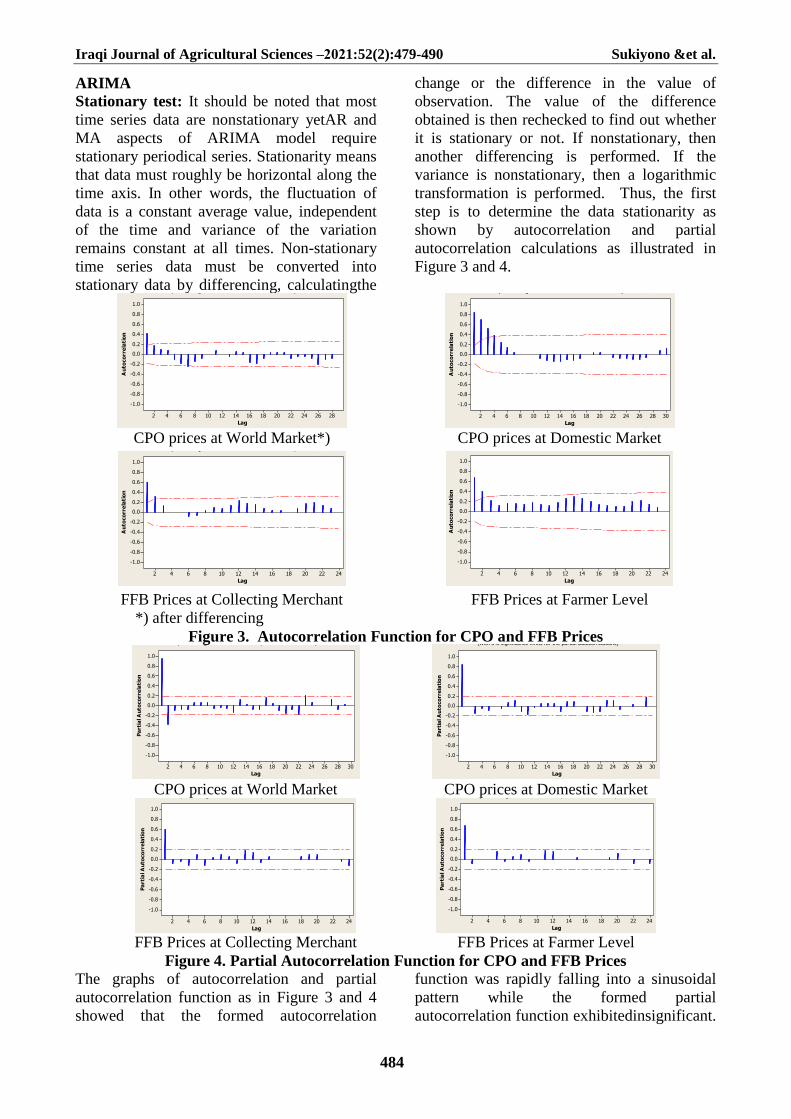
ARIMA
Stationary test: It should be noted that most
time series data are nonstationary yetAR and
MA aspects of ARIMA model require
stationary periodical series. Stationarity means
that data must roughly be horizontal along the
time axis. In other words, the fluctuation of
data is a constant average value, independent
of the time and variance of the variation
remains constant at all times. Non-stationary
time series data must be converted into
stationary data by differencing, calculatingthe
change or the difference in the value of
observation. The value of the difference
obtained is then rechecked to find out whether
it is stationary or not. If nonstationary, then
another differencing is performed. If the
variance is nonstationary, then a logarithmic
transformation is performed. Thus, the first
step is to determine the data stationarity as
shown by autocorrelation and partial
autocorrelation calculations as illustrated in
Figure 3 and 4.
282624222018161412108642
1.0
0.8
0.6
0.4
0.2
0.0
-0.2
-0.4
-0.6
-0.8
-1.0
Lag
Au
toco
rre
lati
on
Autocorrelation Function for diffrencing(with 5% significance limits for the autocorrelations)
30282624222018161412108642
1.0
0.8
0.6
0.4
0.2
0.0
-0.2
-0.4
-0.6
-0.8
-1.0
Lag
Au
toco
rre
lati
on
Autocorrelation Function for Domestik (Rp/Kg)(with 5% significance limits for the autocorrelations)
CPO prices at World Market*) CPO prices at Domestic Market
24222018161412108642
1.0
0.8
0.6
0.4
0.2
0.0
-0.2
-0.4
-0.6
-0.8
-1.0
Lag
Au
toco
rre
lati
on
Autocorrelation Function for Pengumpul (Rp/Kg)(with 5% significance limits for the autocorrelations)
24222018161412108642
1.0
0.8
0.6
0.4
0.2
0.0
-0.2
-0.4
-0.6
-0.8
-1.0
Lag
Au
toco
rre
lati
on
Autocorrelation Function for Petani (Rp/Kg)(with 5% significance limits for the autocorrelations)
FFB Prices at Collecting Merchant FFB Prices at Farmer Level
*) after differencing
Figure 3. Autocorrelation Function for CPO and FFB Prices
30282624222018161412108642
1.0
0.8
0.6
0.4
0.2
0.0
-0.2
-0.4
-0.6
-0.8
-1.0
Lag
Pa
rtia
l A
uto
co
rre
lati
on
Partial Autocorrelation Function for Dunia (USD/Ton)(with 5% significance limits for the partial autocorrelations)
30282624222018161412108642
1.0
0.8
0.6
0.4
0.2
0.0
-0.2
-0.4
-0.6
-0.8
-1.0
Lag
Pa
rtia
l A
uto
co
rre
lati
on
Partial Autocorrelation Function for Domestik (Rp/Kg)(with 5% significance limits for the partial autocorrelations)
CPO prices at World Market CPO prices at Domestic Market
24222018161412108642
1.0
0.8
0.6
0.4
0.2
0.0
-0.2
-0.4
-0.6
-0.8
-1.0
Lag
Pa
rtia
l A
uto
co
rre
lati
on
Partial Autocorrelation Function for Pengumpul (Rp/Kg)(with 5% significance limits for the partial autocorrelations)
24222018161412108642
1.0
0.8
0.6
0.4
0.2
0.0
-0.2
-0.4
-0.6
-0.8
-1.0
Lag
Pa
rtia
l A
uto
co
rre
lati
on
Partial Autocorrelation Function for Petani (Rp/Kg)(with 5% significance limits for the partial autocorrelations)
FFB Prices at Collecting Merchant FFB Prices at Farmer Level
Figure 4. Partial Autocorrelation Function for CPO and FFB Prices
The graphs of autocorrelation and partial
autocorrelation function as in Figure 3 and 4
showed that the formed autocorrelation
function was rapidly falling into a sinusoidal
pattern while the formed partial
autocorrelation function exhibitedinsignificant.

Iraqi Journal of Agricultural Sciences –2021:52(2):479-490 Sukiyono &et al.
485
Furthermore, the model checking done with
Augmented Dickey-Fuller (ADF) unit root test
on CPO and FFB prices confirmedthat the
series was stationary, except for the CPO
prices at the world market. After the first-
difference, the CPO prices at global market
became stationary. Table 2 presents stationary
test for the data used in this paper.
Table 2. Unit Root Test for Stationarity using Augmented Dickey-Fuller
No Data t – statistic Prob Conclusion
1 World Price of CPO -2.8498 0.0553 Non-stationary*)
2 Domestic Prices of CPO -3.1241 0.0281 Stationary
3 FFB at Collecting Merchant -4.7282 0.0002 Stationary
4 FFB at Farmers Level -4.2822 0.0008 Stationary
Estimation of World and Domestic CPO
Prices Model : Due to the non-stationary of
the CPO prices at the world market, these data
hadto be converted into stationary data at the
first differencing. Then, the ARIMA model
for the world CPO prices was estimated. After
comparing all the fit statistics, it is found that
the best model was ARIMA (1,1,2) in which
all the parameters were significant with
respective significant levels as presented in
Table 5. Similar steps were also conducted for
the domestic prices of CPO. It is found that the
best ARIMA model for domestic prices was
ARIMA (1,0,4). The parameters of ARIMA
(1,0,4) with their respective significance
levelsaregivenin Table 3.
Table 3. Estimated Model Parameters of World and Domestic PricesOf CPO
No Data Coefficient SE – Coefficient t – statistic probability
1 World Price of CPO
AR (1) 0.9932 0.0535 18.55 0.000
MA (1) 0.6653 0.0086 76.91 0.000
MA (2) 0.3269 0.1024 3.19 0.002
2 Domestic Prices of CPO
AR (1) 1.0000 0.0002 5023.03 0.000
MA (1) 0.2077 0.0866 2.40 0.018
MA (2) 0.1927 0.0830 2.32 0.039
MA (3) 0.3091 0.0870 3.55 0.001
MA (4) 0.3960 0.0880 4.50 0.000
Estimation of FFB Prices Model
The data of fresh fruit bunch prices, both at
collecting merchant and farmer level were
already stationary, so they did not need a
differencing. From the estimation, it is found
that the best model for the FFB prices at
collecting merchant and farmer level was the
same, i.e., ARIMA (1, 0, 2).
Table 4. Estimated Model Parameters of FFB Prices at Collecting Merchant and Farmer
Level
No Data Coefficient SE – Coefficient t – statistic probability
1 At Collecting Merchant level
AR (1) 1.0002 0.0018 550.43 0.000
MA (1) 0.3951 0.0912 4.33 0.000
MA (2) 0.5061 0.0910 5.56 0.000
2 At Farmer level
AR (1) 1.0003 0.0030 331.99 0.000
MA (1) 0.3663 0.0933 3.93 0.000
MA (2) 0.4677 0.0932 5.02 0.000
Decomposition Model
World and Domestic Prices of CPO
Based on the classical decomposition methods,
the world CPO price forecasting results are
presented in Figure 5 (a) and (b). Looking at
this figure, both additive and multiplicative
methods are likely to produce the same pattern
and results. Looking at the fitted trend
equation, both approaches have similar trends,
i.e., a downward trend with a similar degree of
slope. These results indicate that both methods
can be used to forecast with a similar degree of

Iraqi Journal of Agricultural Sciences –2021:52(2):479-490 Sukiyono &et al.
486
accuracy. This conclusion is supported by the
identical values of MAPE and MAD (Table 5).
MAPE value for both decomposition
forecasting model was 19.70 %, and MAD
value for both models was 156.6. These
inconclusive results imply that forecasters can
use either additive or multiplicative to predict
the world CPO prices. However, if looking at
MSD value, the additive hada smaller MSD
value than multiplicative. The MSD value of
additive decomposition model was 35,731.8
while the MSD value of multiplicative was
35,740.6. This result concludes that additive is
more accurate than commutative in forecasting
the world CPO prices. Based on this
discussion, it is better to apply an additive
decomposition model to forecast the world
CPO prices for the period of January 2007 –
October 2016.
World Prices of CPO
a) Additive Decomposition Model b) Multiplicative Decomposition Model
Domestic Prices of CPO
c) Additive Decomposition Model d) Multiplicative Decomposition Model
Figure 5. Forecasting Results of World and Domestic CPO Prices
The forecasting result of the domestic CPO
prices is presented in Figure 5 (c) and (d). This
figure also indicates that the forecasting results
from additive and multiplicative have similar
patterns and accuracies. The plots tend to
have an upward trend and similar cyclical
patterns. The upward trend of both additive
and multiplicative has positive and quite
similar slope described by its fitted trend
equation. These results also imply that both
forecasting models have a similar degree of
forecasting accuracy. This means
that,regardless of what decomposition models
are used, they will produce identical results.
This conclusion is more convincing when
viewed from the forecasting accuracy
measurements, namely, MAPE and MAD
(Table 5). MAPE and MAD value for both
additive and multiplicative were similar, i.e.,
13 % and 938 respectively. Also, examining
the MSD value, additive decomposition model
was less accurate than multiplicative because
its MSD value was higher than that of
multiplicative, i.e., 1 370 177 for additive and
1 369 277 for multiplicative. For these
reasons, it is better to apply a multiplicative
decomposition model for estimating the future
domestic prices of CPOin Indonesia.
SepAguJulJunMeiAprMarFebJanJan
1300
1200
1100
1000
900
800
700
600
500
400
Month
CP
O W
orld
Pric
e
MAPE 19,7
MAD 156,6
MSD 35731,8
Accuracy Measures
Actual
Fits
Trend
Forecasts
Variable
Time Series Decomposition Plot for CPO World PriceAdditive Model
SepAguJulJunMeiAprMarFebJanJan
11000
10000
9000
8000
7000
6000
5000
Month
Do
me
stic
CP
O P
ric
e
MAPE 13
MAD 988
MSD 1370177
Accuracy Measures
Actual
Fits
Trend
Forecasts
Variable
Time Series Decomposition Plot for Domestic CPO PriceAdditive Model
SepAguJulJunMeiAprMarFebJanJan
11000
10000
9000
8000
7000
6000
5000
Month
Do
me
stic
CP
O P
ric
e
MAPE 13
MAD 988
MSD 1369277
Accuracy Measures
Actual
Fits
Trend
Forecasts
Variable
Time Series Decomposition Plot for Domestic CPO PriceMultiplicative Model
Iraqi Journal of Agricultural Sciences –2021:52(2):479-490 Sukiyono &et al.
487
Table 5. Forecasting Accuracy for World and Domestic CPO Prices Using Decomposition
Forecasting Model Decomposition types MAPE (%) MAD MSD
World Prices
Additive 19.70 156.6 35 731.8
Multiplicative 19.70 156.6 35 740.6
Conclusion Inconclusive Inconclusive Additive
Domestic Prices Additive 13 988 1 370 177
Multiplicative 13 988 1 369 277
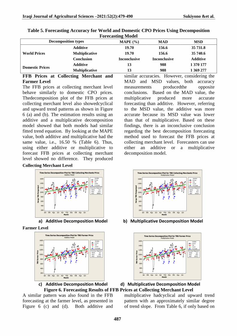
FFB Prices at Collecting Merchant and
Farmer Level
The FFB prices at collecting merchant level
behave similarly to domestic CPO prices.
Thedecomposition plot of the FFB prices at
collecting merchant level also showedcyclical
and upward trend patterns as shown in Figure
6 (a) and (b). The estimation results using an
additive and a multiplicative decomposition
model showed that both models had similar
fitted trend equation. By looking at the MAPE
value, both additive and multiplicative had the
same value, i.e., 16.50 % (Table 6). Thus,
using either additive or multiplicative to
forecast FFB prices at collecting merchant
level showed no difference. They produced
similar accuracies. However, considering the
MAD and MSD values, both accuracy
measurements producedthe opposite
conclusions. Based on the MAD value, the
multiplicative produced more accurate
forecasting than additive. However, referring
to the MSD value, the additive was more
accurate because its MSD value was lower
than that of multiplicative. Based on these
findings, there is an inconclusive conclusion
regarding the best decomposition forecasting
method used to forecast the FFB prices at
collecting merchant level. Forecasters can use
either an additive or a multiplicative
decomposition model.
Collecting Merchant Level
a) Additive Decomposition Model b) Multiplicative Decomposition Model
Farmer Level
c) Additive Decomposition Model d) Multiplicative Decomposition Model Figure 6. Forecasting Results of FFB Prices at Collecting Merchant Level
A similar pattern was also found in the FFB
forecasting at the farmer level, as presented in
Figure 6 (c) and (d). Both additive and
multiplicative hadcyclical and upward trend
pattern with an approximately similar degree
of trend slope. From Table 6, if only based on
JunAguOktDesFebAprJunAguOktJan
1600
1400
1200
1000
800
600
400
200
Month
Ha
rga
TB
S P
en
gu
mp
ul
MAPE 16,5
MAD 154,4
MSD 38898,6
Accuracy Measures
Actual
Fits
Trend
Forecasts
Variable
Time Series Decomposition Plot for TBS Collecting Merchants PriceAdditive Model
JunAguOktDesFebAprJunAguOktJan
1600
1400
1200
1000
800
600
400
200
Month
Ha
rga
TB
S P
en
gu
mp
ul
MAPE 16,5
MAD 153,7
MSD 39154,4
Accuracy Measures
Actual
Fits
Trend
Forecasts
Variable
Time Series Decomposition Plot for TBS Collecting Merchants PriceMultiplicative Model
JunAguOktDesFebAprJunAguOktJan
1600
1400
1200
1000
800
600
400
200
Month
TB
S F
arm
er
Pri
ce
MAPE 16,7
MAD 139,0
MSD 32142,9
Accuracy Measures
Actual
Fits
Trend
Forecasts
Variable
Time Series Decomposition Plot for TBS Farmer PriceAdditive Model
JunAguOktDesFebAprJunAguOktJan
1600
1400
1200
1000
800
600
400
200
Month
TB
S F
arm
er
Pri
ce
MAPE 16,7
MAD 138,4
MSD 32301,2
Accuracy Measures
Actual
Fits
Trend
Forecasts
Variable
Time Series Decomposition Plot for TBS Farmer PriceMultiplicative Model
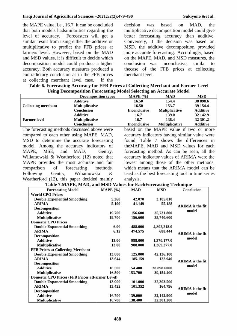
Iraqi Journal of Agricultural Sciences –2021:52(2):479-490 Sukiyono &et al.
488
the MAPE value, i.e., 16.7, it can be concluded
that both models hadsimilarities regarding the
level of accuracy. Forecasters will get a
similar result from using either the additive or
multiplicative to predict the FFB prices at
farmers level. However, based on the MAD
and MSD values, it is difficult to decide which
decomposition model could produce a higher
accuracy. Both accuracy measures produced a
contradictory conclusion as in the FFB prices
at collecting merchant level case. If the
decision was based on MAD, the
multiplicative decomposition model could give
better forecasting accuracy than additive.
Conversely, if the decision was based on
MSD, the additive decomposition provided
more accurate forecasting. Accordingly, based
on the MAPE, MAD, and MSD measures, the
conclusion was inconclusive, similar to
thecase of the FFB prices at collecting
merchant level.
Table 6. Forecasting Accuracy for FFB Prices at Collecting Merchant and Farmer Level
Using Decomposition Forecasting Model Selecting an Accurate Model Decomposition types MAPE (%) MAD MSD
Collecting merchant
Additive 16.50 154.4 38 898.6
Multiplicative 16.50 153.7 39 154.4
Conclusion Inconclusive Multplicative Additive
Farmer level
Additive 16.7 139.0 32 142.9
Multiplicative 16.7 138.4 32 301.2
Conclusion Inconclusive Multiplicative Additive
The forecasting methods discussed above were
compared to each other using MAPE, MAD,
MSD to determine the accurate forecasting
model. Among the accuracy indicators of
MAPE, MSE, and MAD, Gentry,
Wiliamowski & Weatherford (12) noted that
MAPE provides the most accurate and fair
comparison of forecasting methods.
Following Gentry, Wiliamowski &
Weatherford (12), this paper decided mainly
based on the MAPE value if two or more
accuracy indicators having similar value were
found. Table 7 shows the differences in
theMAPE, MAD and MSD values for each
forecasting method. As can be seen, all the
accuracy indicator values of ARIMA were the
lowest among those of the other methods,
which means that the ARIMA model can be
used as the best forecasting tool in time series
analysis.
Table 7.MAPE, MAD, and MSD Values for EachForecasting Technique Forecasting Model MAPE (%) MAD MSD Conclusion
World CPO Prices
Double Exponential Smoothing 5.260 42.070 3,185.010
ARIMA is the fit
model
ARIMA 5.109 41.149 55.188
Decomposition
Additive 19.700 156.600 35,731.800
Multiplicative 19.700 156.600 35,740.600
Domestic CPO Prices
Double Exponential Smoothing 6.00 488.000 4,802,218.0
ARIMA is the fit
model
ARIMA 6.12 474.575 688.444
Decomposition
Additive 13.00 988.000 1,370,177.0
Multiplicative 13.00 988.000 1,369,277.0
FFB Prices at Collecting Merchant
Double Exponential Smoothing 13.800 125.000 42,136.100
ARIMA is the fit
model
ARIMA 13.644 185.159 122.940
Decomposition
Additive 16.500 154.400 38,898.6000
Multiplicative 16.500 153.700 39,154.400
Domestic CPO Prices (FFB Prices atFarmer Level)
Double Exponential Smoothing 13.900 101.000 32,303.500
ARIMA is the fit
model
ARIMA 13.422 101.352 164.796
Decomposition
Additive 16.700 139.000 32,142.900
Multiplicative 16.700 138.400 32,301.200
Iraqi Journal of Agricultural Sciences –2021:52(2):479-490 Sukiyono &et al.
489
To conclude, the primary goal of this study
was to select the most appropriate forecasting
technique for the future prices of CPO prices,
both at domestic and world markets, and FFB
prices at collecting merchant and farmer level
in Bengkulu Province. Three types of
forecasting methods were used in this study,
namely, double exponential smoothing,
ARIMA, and classical decomposition
methods. The forecasting method was selected
by least forecasting errors, that is, minimum
values of MAPE, MAD, as well as MSD.
Even though some decision is not always
unanimous, it is found that the ARIMA model
provides the most accurate prediction for CPO
and FFB prices based on most of the accuracy
measures.
REFERENCES
1. Adebiyi, A. A., A. O., Adewumi, and C. K.
Ayo, 2014. Stock Price Prediction Using the
ARIMA Model. Paper presented at 2014
UKSim-AMSS 16th International Conference
on Computer Modelling and Simulation. DOI:
10.1109/UKSim.2014.67
2. Bowerman, B. L., R. T., O’Connell, and A.
B. Koehler, 2004. Forecasting, time series, and
regression: An applied approach. Belmont,
CA7 Thomson Brooks/Cole
3. Bowman, C. and A. Husain, 2004.
Forecasting Commodity Prices: Futures
Versus Judgment (March 2004). IMF Working
Paper No. 04/41. Available at SSRN:
https://ssrn.com/abstract=878864
4. Box, G. E. P. and G. M.. Jenkins,
1976.Time Series AnalysisForecasting and
Control, Third ed. Englewood Cliffs, NJ:
Prentice-Hall
5. Calantone, R. J., A., Di Benedetto, and D.
Bojanic, 1987. A comprehensivereview of the
tourism forecasting literature. Journal of
TravelResearch, 26(2), 28–
39.https://doi.org/10.1177/0047287587026002
07
6. Cleveland, R. B., W. S.,Cleveland, J. E.
McRae, and I. Terpenning, 1990. STL: A
Seasonal-Trend Decomposition Procedure
Based on Loess (with Discussion). Journal of
Official Statistics, 6, 3-73.
7. Directorate General of Estate Crops. 2016.
Statistik Perkebunan Indonesia: Kelapa Sawit
2015 – 2017. Jakarta
8. Gauch, H. G., Jr., J. T. Hwang, and G. W.
G.and Fick, 2003. Model Evaluation by
Comparison of Model-Based Predictions and
Measured Values. Agronomy Journal, 95
(November–December2003), 1442 – 1446.
Retrieved from
www2.geog.ucl.ac.uk/~mdisney/.../gauch_mod
el_eval.pdf
9. Gentry, T. W., B. M. Wiliamowski, and L.
R. Weatherford, 1995. A Comparison of
Traditional Forecasting Technique and Neutral
Network. Retrieved from
http://www.eng.auburn.edu/~wilambm/pap/19
95/ANNIE'95_A_comparison_of_traditional_f
orecasting.pdf
10. Hanke, J. E., and A. G. Reitsch, 1995.
Business Forecasting (5th
ed.). Englewood
Cliffs, NJ7 Prentice-Hall
11. Hanke, J.E., A.G., Reitsch, and D.W.
Wichern, 2003. Business Forecasting Seventh
Edition, Williams Publishers
12. Hyndman, R. J. 2009. Forecasting
overview. November 8, 2009, available at
https://robjhyndman.com/papers/forecastingov
erview.pdf
13. Hyndman, R. J. and A. B. Koehler, 2006.
Another look at measures of forecast accuracy.
International Journal of Forecasting. 22, 679 –
688. DOI:10.1016/j.ijforecast.2006.03.001
14. Infosawit (11 September 2015).Accessed
from https://www.infosawit.com/.../harga-tbs-
jambi-naik--periode-11-17-september-2015
15. Jha, G. K. and K. Sinha, 2013.
Agricultural Price Forecasting Using Neural
Network Model: AnInnovative Information
Delivery System. Agricultural Economics
Research Review. 26 (2) July-December
2013: 229–239. Retrieved from
https://ageconsearch.umn.edu/bitstream/16215
0/2/8-GK-Jha.pdf
16. Kalekar, P. S. 2004. Time series
Forecasting using Holt-Winters Exponential
Smoothing. Kanwal Rekhi School of
Information Technology. Available at
https://labs.omniti.com/people/jesus/papers/hol
twinters.pdf
17. Khan, T. F., Sayem, S. M. and M. S.
Jahan, 2010. Forecasting price of selected
agricultural commodities In Bangladesh: An
Empirical Study. ASA University Review,
January–June 2010 4(1): 15 – 22. Retrieved
from

Iraqi Journal of Agricultural Sciences –2021:52(2):479-490 Sukiyono &et al.
490
http://www.asaub.edu.bd/data/asaubreview/v4
n1sl2.pdf
18. Krajewski, L. J., and L. P. Ritzman, 1993.
Operations Management: Strategy and
Analysis, 5th
Edition. Pearson
19. Lim, P. Y. and C. V. Nayar, 2012. Solar
irradiance and load demand forecasting based
on single exponentialsmoothing
method.International Journal of Engineering
and Technology. 4(4):451 – 455. DOI:
10.7763/IJET.2012.V4.408 Retrieved from
www.ijetch.org/papers/408-P016.pdf
20. Makridakis, S., S. C. Wheelwright, and R.
J. Hyndman. 1998. Forecasting Methods and
Applications. New York, John Wiley and Sons
21. Pankratz, A. 1983.Forecasting with
Univariate Box–Jenkinsmodels: concepts and
cases. New York: John Wiley & Sons
22. Peng, W. Y. and C. W. Chu, 2009. A
comparison of univariate methods for
forecasting container throughput volumes.
Mathematical and Computer Modelling. 50
(2009), 1045 – 1057. https:// doi.org/
10.1016/j.mcm.2009.05.027
23. Rajchakit, M. 2017. A New Method for
Forecasting via FeedbackControl Theory.
Proceedings of the International
MultiConference of Engineers and Computer
Scientists 2017 Vol I,IMECS 2017, March 15
- 17, 2017, Hong Kong. Retrieved from
http://www.iaeng.org/publication/IMECS2017
24. Sensus Pertanian. 2013. Laporan
HasilSensus Pertanian2013. BPS Jakarta
25. Sriboonchitta, S., H. T., Nguyen, A.,
Wiboonpongse, and J. Liu, 2013. Modeling
volatility and dependency of agricultural price
and production indices of Thailand: Static
versus time-varying copulas. International
Journal of Approximate Reasoning 54, 793 –
808.
http://dx.doi.org/10.1016/j.ijar.2013.01.004
26. Stevenson, W. J. 2009. Operations
Management, 10th edition, Mc Graw Hill Inc,
New York
27. Sukiyono, K. and Rosdiana. 2018.
Pendugaan model peramalan harga beras pada
Tingkat grosir. agrisep 17(1), 23 – 30. DOI:
10.31186/jagrisep. 17.1.23-30. Retrieved
mfrom https:// ejournal.unib.
ac.id/index.php/agrisep/article/view/4503 /pdf
28. Sukiyono, K.,I. Cahyadinata, A. Purwoko,
S. Widiono,E. Sumartono, N.N.Arianti, and G.
Mulyasari, 2017. Assessing smallholder
household vulnerability to price volatility
ofPalm fresh fruit bunch in Bengkulu
Province. International Journal of Applied
Business and Economic Research. 15(3), 1 –
15.http://www.serialsjournals.com/serialjourna
lmanager/pdf/1490596894.pdf
29. Sukiyono, K., M. Z. S.P. Yuliarso, E.
Utama, R. Yuliarti, R.Novanda, and B.
S.Priyono. (2019). Possible method For
monthly naturalRubber price forecasting.
Journal of Advanced Research in Dynamical
and Control Systems – Jardcs, 11, (Issue-07):
387 – 395. 2019. https:// www.jardcs.org
/abstract. php?id=2555
30. Taylor, J. 2003. Short-term electricity
demand forecasting using double seasonal
exponential smoothing. The Journal of the
Operational Research Society,54(8), 799-805.
Retrieved from
http://www.jstor.org/stable/4101650
31. Taylor, J. W. 2008. An evaluation of
methods for very short-term load
forecastingusing minute-by-minute British
data. International Journal of Forecasting. 24,
645– 658 https:/ /doi.org/ 10.1016/j
.ijforecast.2008.07.007
32. Xin, W. and W.Can, 2016. Empirical study
on agricultural products price forecasting
based on internet-based Timely price
information. International Journal of
Advanced Science and Technology. 87, 31-36.
http://dx.doi.org/10.14257/ijast.2016.87.04.