A model reduction approach to numerical inversion for a

A model reduction approach to numerical inversionfor a parabolic partial differential equation

Alexander V. Mamonov1,Liliana Borcea2, Vladimir Druskin3

and Mikhail Zaslavsky3

1Schlumberger and the University of Texas at Austin (ICES)2University of Michigan, Ann Arbor

3Schlumberger-Doll Research Center

Support: NSF DMS-0934594.

A.V. Mamonov (Schlumberger) Model Reduction for Inversion 1 / 38

A model reduction approach to numerical inversion fora parabolic partial differential equation

1 Problem formulation

2 Model order reduction and inversion

3 Matching conditions

4 Non-linear preconditioner and its Jacobian

5 Inversion method and numerical results

6 Extension to two dimensions

7 Conclusions and future work


Problem formulation

MotivationProblem: Time-domain Controlled Source Electromagnetic (CSEM) methodin oil and gas exploration

Determine the resistivity in the subsurface from time-resolved surfacemeasurements

Quasi-stationary parabolic Maxwell system

Highly non-linear inverse problem, local minima, slow convergence

Expensive forward modeling

Figures from: http://www.acceleware.com, http://www.engineerlive.com/Mining-Engineer/CSEM


http://www.acceleware.com

http://www.engineerlive.com/Mining-Engineer/CSEM

Problem formulation

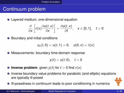
Continuum problem

Layered medium, one-dimensional equation

∂

∂x

[r(x)

∂u(t , x)

∂x

]=∂u(t , x)

∂t, x ∈ [0,1], t > 0

Boundary and initial conditions

ux (t ,0) = u(t ,1) = 0, u(0, x) = δ(x)

Measurements: boundary time-domain response

y(t) = u(t ,0), t > 0

Inverse problem: given y(t) for t > 0 find r(x)

Inverse boundary value problems for parabolic (and elliptic) equationsare typically ill-posed

Ill-posedness in continuum leads to poor conditioning in numerics


Model order reduction and inversion

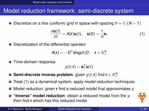
Model reduction framework: semi-discrete system

Discretize on a fine (uniform) grid in space with spacing h = 1/(N + 1)

∂u(t)∂t

= A(r)u(t), u(0) =1h

e1 (1)

Discretization of the differential operator

A(r) = −DT diag(r)D, r ∈ RN+

Time-domain responsey(t ; r) = eT

1 u(t)

Semi-discrete inverse problem: given y(t ; r) find r ∈ RN+

Treat (1) as a dynamical system, apply model reduction techniques

Model reduction: given r find a reduced model that approximates y

“Inverse” model reduction: obtain a reduced model from the y ,then find r which has this reduced model



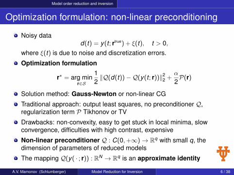
Optimization formulation: non-linear preconditioning

Noisy datad(t) = y(t ; rtrue) + ξ(t), t > 0,

where ξ(t) is due to noise and discretization errors.

Optimization formulation

r? = arg minr∈S

12‖Q(d(t))−Q(y(t ; r))‖2

2 +α

2P(r)

Solution method: Gauss-Newton or non-linear CG

Traditional approach: output least squares, no preconditioner Q,regularization term P Tikhonov or TV

Drawbacks: non-convexity, easy to get stuck in local minima, slowconvergence, difficulties with high contrast, expensive

Non-linear preconditioner Q : C(0,+∞)→ Rq with small q, thedimension of parameters of reduced models

The mapping Q(y( · ; r)) : RN → Rq is an approximate identity



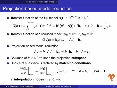
Projection-based model reduction

Transfer function of the full model A(r) ∈ RN×N , b ∈ RN

G(s; r) =

∫ +∞

0y(t ; r)e−stdt = bT (sI − A(r))−1b, s > 0, b =

1√h

e1

Transfer function of a reduced model Am ∈ Rm×m, bm ∈ Rm

Gm(s) = bTm(sIm − Am)−1bm

Projection-based model reduction

Am = V T AV , bm = V T b, V T V = Im

Columns of V ∈ RN×m span the projection subspace

Choice of subspace is dictated by matching conditions

∂k Gm

∂sk

∣∣∣∣s=σj

=∂k G∂sk

∣∣∣∣s=σj

, j = 1, . . . ,m, k = 0, . . . ,2Mj − 1

at interpolation nodes σj ∈ [0,+∞)



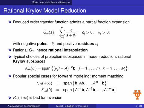
Rational Krylov Model Reduction

Reduced order transfer function admits a partial fraction expansion

Gm(s) =m∑

j=1

cj

s + θj, cj > 0, θj > 0,

with negative poles −θj and positive residues cj

Rational Gm, hence rational interpolation

Typical choices of projection subspaces in model reduction: rationalKrylov subspaces

Km(σ) = span{

(σj I − A)−k b | j = 1, . . . ,m; k = 1, . . . ,Mj}

Popular special cases for forward modeling: moment matching

Km(+∞) = span{

b,Ab, . . . ,Am−1b}

Km(0) = span{

A−1b,A−2b, . . . ,A−mb}

Km(+∞) is bad for inversion



Inversion via model reduction: H2-optimality

Proposed in [Druskin, Simoncini, Zaslavsky, 2011]

Based on H2-optimal reduced models

View reduced model as a function of interpolation nodes σ

ym(t ;σ) = bT V (σ)eAm(σ)tV (σ)T b, for Am(σ) = V (σ)T A(r)V (σ)

Minimize time-domain error in L2 sense

σ? = arg min‖y(t ; r)− ym(t ;σ)‖L2[0,+∞)

Equivalent to H2-optimality in Laplace domain (solve with IRKA)

σ? = arg min‖G(s; r)−Gm(s)‖H2

Use poles and residues of Gm(s) as parameters in inversion

Define the non-linear preconditioner with a chain of mappings

QH2(y( · ; r)) : r (a)→ A(r)

(b)→ σ?(c)→ V (σ?)

(d)→ Am(e)→ {(cj , θj )}m

j=1



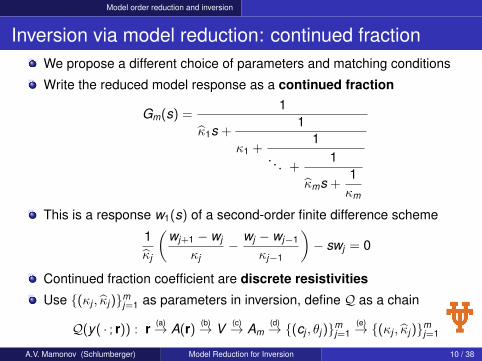
Inversion via model reduction: continued fractionWe propose a different choice of parameters and matching conditions

Write the reduced model response as a continued fraction

Gm(s) =1

κ̂1s +1

κ1 +1

. . . +1

κ̂ms +1κm

This is a response w1(s) of a second-order finite difference scheme

1κ̂j

(wj+1 − wj

κj−

wj − wj−1

κj−1

)− swj = 0

Continued fraction coefficient are discrete resistivities

Use {(κj , κ̂j )}mj=1 as parameters in inversion, define Q as a chain

Q(y( · ; r)) : r (a)→ A(r)(b)→ V (c)→ Am

(d)→ {(cj , θj )}mj=1

(e)→ {(κj , κ̂j )}mj=1


Matching conditions

Matching conditions for inversion

The choice of matching conditions is important: what is good for forwardmodeling is not necessarily good for inversion

Use the Jacobian of Q to quantify the quality of matching conditions

(DQ)j,k =

∂κj

∂rk, for j = 1, . . . ,m

∂κ̂j

∂rk, for j = m + 1, . . . ,2m

, k = 1, . . . ,N.

Proper matching conditions should give good conditioning andresolution

Good conditioning of DQ is desirable for fast and robust performance ofGauss-Newton iteration, possible to achieve cond(DQ) ≈ O(1)

Conditioning of Q(d( · )) always grows exponentially (unavoidableill-posedness), slower growth is preferential

Resolution is connected to optimal grids


Matching conditions

Connection to optimal grids

Optimal (spectrally matched) grids were introduced in [Druskin,Knizhnerman, 2000] for exponential superconvergence of DtN maps

Typically defined for r(x) ≡ 1

(κ(0)j , κ̂

(0)j )m

j=1 = Q(y( · , r(0))), r(0) = (1,1, . . . ,1)T

Continued fraction coefficients are the grid steps of FD scheme for

∆w − sw = 0

Staggered grid with primary and dual nodes

x (0)j =

j∑k=1

κ(0)k , x̂ (0)

j =

j∑k=1

κ̂(0)k , j = 1, . . . ,m

Optimal grids were used for inversion (Sturm-Liouville, EIT)

Here we do not explicitly use optimal grids for inversion,but to quantify the resolution


Matching conditions

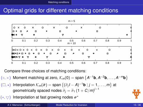
Optimal grids for different matching conditions

0 0.1 0.2 0.3 0.4 0.5 0.6 0.7 0.8 0.9 1

m = 5

0 0.1 0.2 0.3 0.4 0.5 0.6 0.7 0.8 0.9 1

m = 10

Compare three choices of matching conditions:

(◦,×) Moment matching at zero, Km(0) = span{

A−1b,A−2b, . . . ,A−mb}

(�, ?) Interpolation Km(σ̃) = span{

(σ̃j I − A)−1b | j = 1, . . . ,m}

atgeometrically spaced nodes σ̃j = σ̃1 (1 + C/m)j−1

(∗,5) Interpolation at fast growing nodes σ?


Matching conditions

Conditioning of the Jacobian

2 3 4 5 6 7 8 9 10 11 12 1310

0

101

102

103

104

105

106

m

cond(D

Q)

Rows of DQ have themeaning of sensitivityfunctions

Each row correspondsto one grid cell

Sensitivity functionsare localized

Peak locations are atthe optimal grid nodes

Clustered nodes leadto (almost) linearlydependent rows of DQ

Condition number growth for moment matching at zero (◦),interpolation at σ̃ (�), interpolation at σ? (5)


Matching conditions

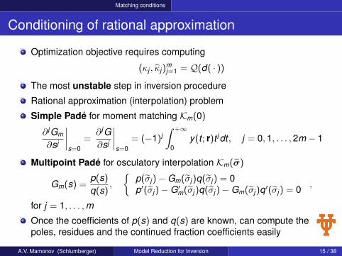
Conditioning of rational approximation

Optimization objective requires computing

(κj , κ̂j )mj=1 = Q(d( · ))

The most unstable step in inversion procedure

Rational approximation (interpolation) problem

Simple Padé for moment matching Km(0)

∂ jGm

∂sj

∣∣∣∣s=0

=∂ jG∂sj

∣∣∣∣s=0

= (−1)j∫ +∞

0y(t ; r)t jdt , j = 0,1, . . . ,2m − 1

Multipoint Padé for osculatory interpolation Km(σ̃)

Gm(s) =p(s)

q(s),

{p(σ̃j )−Gm(σ̃j )q(σ̃j ) = 0p′(σ̃j )−G′m(σ̃j )q(σ̃j )−Gm(σ̃j )q′(σ̃j ) = 0 ,

for j = 1, . . . ,m

Once the coefficients of p(s) and q(s) are known, can compute thepoles, residues and the continued fraction coefficients easily


Matching conditions

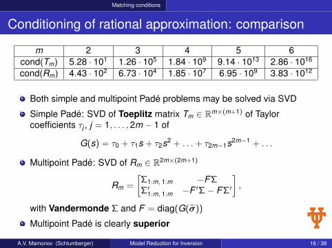
Conditioning of rational approximation: comparison

m 2 3 4 5 6cond(Tm) 5.28 · 101 1.26 · 105 1.84 · 109 9.14 · 1013 2.86 · 1016

cond(Rm) 4.43 · 102 6.73 · 104 1.85 · 107 6.95 · 109 3.83 · 1012

Both simple and multipoint Padé problems may be solved via SVD

Simple Padé: SVD of Toeplitz matrix Tm ∈ Rm×(m+1) of Taylorcoefficients τj , j = 1, . . . ,2m − 1 of

G(s) = τ0 + τ1s + τ2s2 + . . .+ τ2m−1s2m−1 + . . .

Multipoint Padé: SVD of Rm ∈ R2m×(2m+1)

Rm =

[Σ1:m, 1:m −FΣΣ′1:m, 1:m −F ′Σ− FΣ′

],

with Vandermonde Σ and F = diag(G(σ̃))

Multipoint Padé is clearly superior


Non-linear preconditioner and its Jacobian

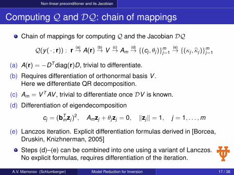
Computing Q and DQ: chain of mappings

Chain of mappings for computing Q and the Jacobian DQ

Q(y( · ; r)) : r (a)→ A(r)(b)→ V (c)→ Am

(d)→ {(cj , θj )}mj=1

(e)→ {(κj , κ̂j )}mj=1

(a) A(r) = −DT diag(r)D, trivial to differentiate.

(b) Requires differentiation of orthonormal basis V .Here we differentiate QR decomposition.

(c) Am = V T AV , trivial to differentiate once DV is known.

(d) Differentiation of eigendecomposition

cj = (bTmzj )

2, Amzj + θjzj = 0, ‖zj‖ = 1, j = 1, . . . ,m

(e) Lanczos iteration. Explicit differentiation formulas derived in [Borcea,Druskin, Knizhnerman, 2005]

Steps (d)–(e) can be combined into one using a variant of Lanczos.No explicit formulas, requires differentiation of the iteration.


Non-linear preconditioner and its Jacobian

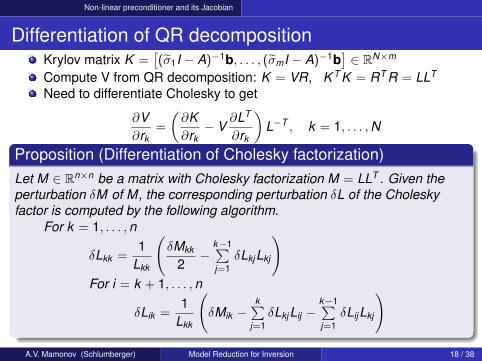
Differentiation of QR decompositionKrylov matrix K =

[(σ̃1I − A)−1b, . . . , (σ̃mI − A)−1b

]∈ RN×m

Compute V from QR decomposition: K = VR, K T K = RT R = LLT

Need to differentiate Cholesky to get

∂V∂rk

=

(∂K∂rk− V

∂LT

∂rk

)L−T , k = 1, . . . ,N

Proposition (Differentiation of Cholesky factorization)Let M ∈ Rn×n be a matrix with Cholesky factorization M = LLT . Given theperturbation δM of M, the corresponding perturbation δL of the Choleskyfactor is computed by the following algorithm.

For k = 1, . . . ,n

δLkk =1

Lkk

(δMkk

2−

k−1∑j=1

δLkjLkj

)For i = k + 1, . . . ,n

δLik =1

Lkk

(δMik −

k∑j=1

δLkjLij −k−1∑j=1

δLijLkj

)


Inversion method and numerical results

Regularization

Traditional approaches require regularization for stability

We use regularization only to improve the reconstruction quality

Separate the fitting ‖Q(d( · ))−Q(y( · ; r)‖2 step from regularization step

Jacobian DQ ∈ R2m×N has a large null space 2m� N

Minimze the regularization functional P(r) in null(DQ)

Weighted discrete H1 seminorm

P(r) =12‖W 1/2∆r‖2

2,

here ∆ is the truncation of D (first derivative, not second)

Works for both smooth (W = I) and piecewise constant resistivities(non-linear re-weighting at every iteration)

Constrained optimization subproblem at each Gauss-Newton iteration

minimizes.t. [DQ](r−ρ)=0

ρT ∆T W ∆ρ



Regularization

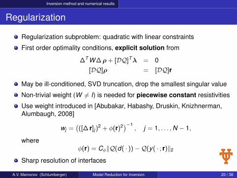
Regularization subproblem: quadratic with linear constraints

First order optimality conditions, explicit solution from

∆T W ∆ρ + [DQ]Tλ = 0[DQ]ρ = [DQ]r

May be ill-conditioned, SVD truncation, drop the smallest singular value

Non-trivial weight (W 6= I) is needed for piecewise constant resistivities

Use weight introduced in [Abubakar, Habashy, Druskin, Knizhnerman,Alumbaugh, 2008]

wj =(([∆ r]j )

2 + φ(r)2)−1, j = 1, . . . ,N − 1,

whereφ(r) = Cφ‖Q(d( · ))−Q(y( · ; r)‖2

Sharp resolution of interfaces



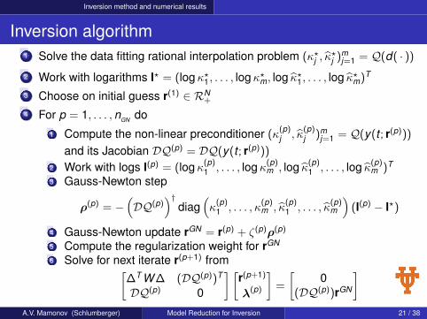
Inversion algorithm1 Solve the data fitting rational interpolation problem (κ?j , κ̂

?j )m

j=1 = Q(d( · ))

2 Work with logarithms l? = (logκ?1, . . . , logκ?m, log κ̂?1, . . . , log κ̂?m)T

3 Choose on initial guess r(1) ∈ RN+

4 For p = 1, . . . ,nGN do

1 Compute the non-linear preconditioner (κ(p)j , κ̂

(p)j )m

j=1 = Q(y(t ; r(p)))

and its Jacobian DQ(p) = DQ(y(t ; r(p)))

2 Work with logs l(p) = (logκ(p)1 , . . . , logκ(p)m , log κ̂(p)1 , . . . , log κ̂(p)m )T

3 Gauss-Newton step

ρ(p) = −(DQ(p)

)†diag

(κ(p)1 , . . . , κ

(p)m , κ̂

(p)1 , . . . , κ̂

(p)m

)(l(p) − l?)

4 Gauss-Newton update rGN = r(p) + ζ(p)ρ(p)

5 Compute the regularization weight for rGN

6 Solve for next iterate r(p+1) from[∆T W ∆ (DQ(p))T

DQ(p) 0

] [r(p+1)

λ(p)

]=

[0

(DQ(p))rGN

]A.V. Mamonov (Schlumberger) Model Reduction for Inversion 21 / 38


Numerical experiments: setupTime stepping over [0,Tmax] with NT steps to compute y ∈ RNT

Systematic discretization errors even in the absence of noise

yj = y(tj ; rtrue) + ξ(s)(tj ), j = 1, . . . ,NT

Generate the data by adding noise d = y + ξ(n)

Noise modelξ(n) = εdiag(χ1, . . . , χNT )y,

with independent χk ∈ N (0,1)

Reduced model size m chosen based on noise level ε

m 3 4 5 6ε 5 · 10−2 5 · 10−3 10−4 0 (noiseless)

Relative `2 error to measure the quality

E =‖r? − rtrue‖2

‖rtrue‖2

Initial guess r1 = 1, five Gauss-Newton iterations nGN = 5A.V. Mamonov (Schlumberger) Model Reduction for Inversion 22 / 38


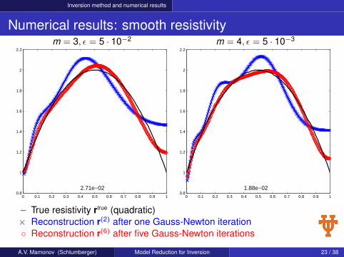
Numerical results: smooth resistivitym = 3, ε = 5 · 10−2 m = 4, ε = 5 · 10−3

0 0.1 0.2 0.3 0.4 0.5 0.6 0.7 0.8 0.9 10.8

1

1.2

1.4

1.6

1.8

2

2.2

2.71e−020 0.1 0.2 0.3 0.4 0.5 0.6 0.7 0.8 0.9 1

0.8

1

1.2

1.4

1.6

1.8

2

2.2

1.88e−02

– True resistivity rtrue (quadratic)× Reconstruction r(2) after one Gauss-Newton iteration◦ Reconstruction r(6) after five Gauss-Newton iterations



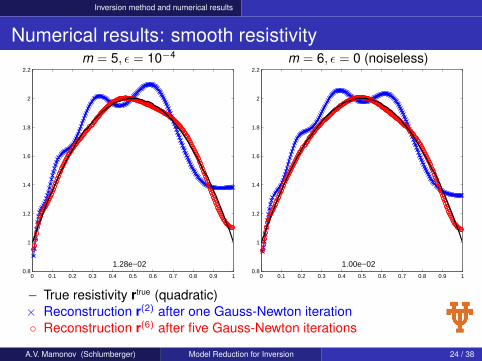
Numerical results: smooth resistivitym = 5, ε = 10−4 m = 6, ε = 0 (noiseless)

0 0.1 0.2 0.3 0.4 0.5 0.6 0.7 0.8 0.9 10.8

1

1.2

1.4

1.6

1.8

2

2.2

1.28e−020 0.1 0.2 0.3 0.4 0.5 0.6 0.7 0.8 0.9 1

0.8

1

1.2

1.4

1.6

1.8

2

2.2

1.00e−02

– True resistivity rtrue (quadratic)× Reconstruction r(2) after one Gauss-Newton iteration◦ Reconstruction r(6) after five Gauss-Newton iterations



Numerical results: smooth resistivitym = 3, ε = 5 · 10−2 m = 4, ε = 5 · 10−3

0 0.1 0.2 0.3 0.4 0.5 0.6 0.7 0.8 0.9 10.8

1

1.2

1.4

1.6

1.8

2

2.2

4.31e−020 0.1 0.2 0.3 0.4 0.5 0.6 0.7 0.8 0.9 1

0.8

1

1.2

1.4

1.6

1.8

2

2.2

2.00e−02

– True resistivity rtrue (linear + Gaussian)× Reconstruction r(2) after one Gauss-Newton iteration◦ Reconstruction r(6) after five Gauss-Newton iterations



Numerical results: smooth resistivitym = 5, ε = 10−4 m = 6, ε = 0 (noiseless)

0 0.1 0.2 0.3 0.4 0.5 0.6 0.7 0.8 0.9 10.8

1

1.2

1.4

1.6

1.8

2

2.2

1.36e−020 0.1 0.2 0.3 0.4 0.5 0.6 0.7 0.8 0.9 1

0.8

1

1.2

1.4

1.6

1.8

2

2.2

1.05e−02

– True resistivity rtrue (linear + Gaussian)× Reconstruction r(2) after one Gauss-Newton iteration◦ Reconstruction r(6) after five Gauss-Newton iterations



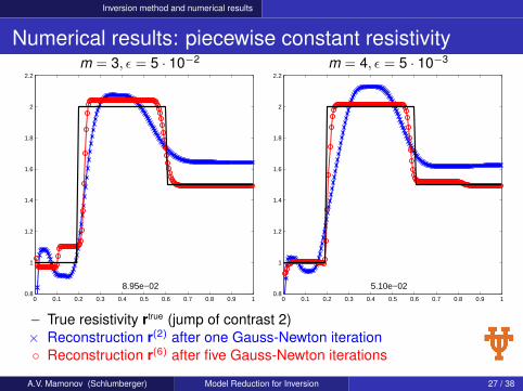
Numerical results: piecewise constant resistivitym = 3, ε = 5 · 10−2 m = 4, ε = 5 · 10−3

0 0.1 0.2 0.3 0.4 0.5 0.6 0.7 0.8 0.9 10.8

1

1.2

1.4

1.6

1.8

2

2.2

8.95e−020 0.1 0.2 0.3 0.4 0.5 0.6 0.7 0.8 0.9 1

0.8

1

1.2

1.4

1.6

1.8

2

2.2

5.10e−02

– True resistivity rtrue (jump of contrast 2)× Reconstruction r(2) after one Gauss-Newton iteration◦ Reconstruction r(6) after five Gauss-Newton iterations



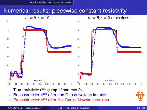
Numerical results: piecewise constant resistivitym = 5, ε = 10−4 m = 6, ε = 0 (noiseless)

0 0.1 0.2 0.3 0.4 0.5 0.6 0.7 0.8 0.9 10.8

1

1.2

1.4

1.6

1.8

2

2.2

6.00e−020 0.1 0.2 0.3 0.4 0.5 0.6 0.7 0.8 0.9 1

0.8

1

1.2

1.4

1.6

1.8

2

2.2

3.56e−02

– True resistivity rtrue (jump of contrast 2)× Reconstruction r(2) after one Gauss-Newton iteration◦ Reconstruction r(6) after five Gauss-Newton iterations


Extension to two dimensions

Approaches to higher dimensions

Higher dimensions:

One-dimensional problem is formally determined: 1D unknown r(x) and1D data y(t)

In dimension two the problem is already overdetermined: 2D unknownr(x , y), but 3D data yi,j (t), where (i , j) are source-detector pairs

Straightforward generalization: block Lanczos, block Krylov subspaces,matrix-valued continued fractions

Block tridiagonal matrix with dense blocks, consequence of anoverdetermined problem

Dense blocks do not correspond directly to a finite-difference scheme

Work with a subset of the data, make the problem formally determined



Coinciding sources and receivers (transducers)

Using one scalar continued fraction per transducer:

Simplest reduction of the data yi,j (t): take the diagonal i = j

Sources and receivers coincide

Excite at a point on the boundary at t = 0, measure yj (t) at the samelocation for t > 0 for each transducer j = 1, . . . ,n

Not the best setting in practice, measurements at source locations maybe noisy

Easier to work with theoretically, coinciding sources/receivers preservethe symmetry

Construct separate scalar continued fractions interpolating each yj (t),j = 1, . . . ,n

Continued fractions are again Stieltjes due to the symmetry



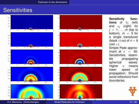
SensitivitiesSensitivity func-tions of κ̂j (left)and κj (right) forj = 1, . . . ,m (top tobottom), m = 5 fora single transducer(black ◦) out of n = 8(red ×).Simple Pade approx-imant at σ = 60.Sensitivities resem-ble propagatingspherical waves.Higher σ meanslower speed ofpropagation. Shouldavoid reflections fromboundaries.



Reconstructions: single low contrast inclusion

0 0.5 1 1.5 2 2.5 30

0.2

0.4

0.6

0.8

1

1

1.2

1.4

1.6

1.8

2

0 0.5 1 1.5 2 2.5 30

0.2

0.4

0.6

0.8

1

1

1.5

2

Top: true r(x , y). Bottom: reconstruction after a single Gauss-Newtoniteration. Constant initial guess r0(x , y) ≡ 1. Transducers: red ×.A.V. Mamonov (Schlumberger) Model Reduction for Inversion 32 / 38


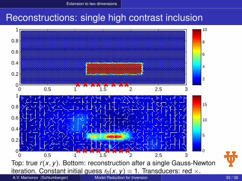
Reconstructions: single high contrast inclusion

0 0.5 1 1.5 2 2.5 30

0.2

0.4

0.6

0.8

1

2

4

6

8

10

0 0.5 1 1.5 2 2.5 30

0.2

0.4

0.6

0.8

1

0

5

10

15



Reconstructions: two adjacent inclusions

0 0.5 1 1.5 2 2.5 30

0.2

0.4

0.6

0.8

1

0.5

1

1.5

2

0 0.5 1 1.5 2 2.5 30

0.2

0.4

0.6

0.8

1

0.5

1

1.5

2



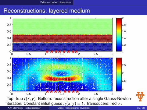
Reconstructions: layered medium

0 0.5 1 1.5 2 2.5 30

0.2

0.4

0.6

0.8

1

1

1.2

1.4

1.6

1.8

2

0 0.5 1 1.5 2 2.5 30

0.2

0.4

0.6

0.8

1

1

1.5

2

2.5



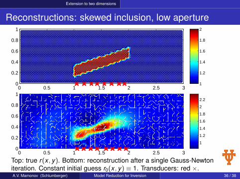
Reconstructions: skewed inclusion, low aperture

0 0.5 1 1.5 2 2.5 30

0.2

0.4

0.6

0.8

1

1

1.2

1.4

1.6

1.8

2

0 0.5 1 1.5 2 2.5 30

0.2

0.4

0.6

0.8

1

1

1.2

1.4

1.6

1.8

2

2.2



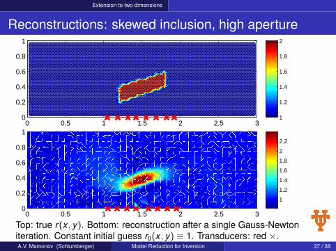
Reconstructions: skewed inclusion, high aperture

0 0.5 1 1.5 2 2.5 30

0.2

0.4

0.6

0.8

1

1

1.2

1.4

1.6

1.8

2

0 0.5 1 1.5 2 2.5 30

0.2

0.4

0.6

0.8

1

1

1.2

1.4

1.6

1.8

2

2.2


Conclusions and future work

Conclusions and future work

Conclusions:Non-linear preconditioning based on model reductionData fitting: rational interpolation (unavoidably ill-conditioned)Reconstruction: well-conditionedFast convergence, inexpensivePossible to extend to higher dimensions

Future work:More work on 2D and 3DNon-coinciding source-receiver pairsDeal with the loss of symmetry

Preprint: A model reduction approach to numerical inversion for aparabolic partial differential equation. L. Borcea, V. Druskin,A.V. Mamonov and M. Zaslavsky, 2012, arXiv:1210.1257 [math.NA]


Documents

A model reduction approach to numerical inversion for a