A model of perceptual constancy based on acoustic feature selection

Guy Brown and Kalle Palomäki

5th July 2011

1

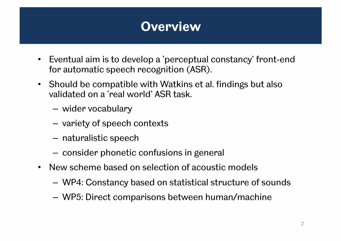
Overview

•  Eventual aim is to develop a ‘perceptual constancy’ front-end for automatic speech recognition (ASR).

•  Should be compatible with Watkins et al. findings but also validated on a ‘real world’ ASR task.

–  wider vocabulary

–  variety of speech contexts

–  naturalistic speech

–  consider phonetic confusions in general

•  New scheme based on selection of acoustic models

–  WP4: Constancy based on statistical structure of sounds

–  WP5: Direct comparisons between human/machine

2

Reminder: Amy’s experiment

•  Amy’s first experiment used 80 utterances from the Articulation Index corpus –  20 instances each of “sir”, “skur”, “spur” and “stir” test

words –  Test word embedded in 3 context words

•  Overall confusion rate was controlled by lowpass filtering at 1, 1.5, 2, 3 and 4 kHz (here we consider 4kHz condition only)

•  Same reverberation conditions as in Watkins et al. experiments

Test 0.32m Test 10m

Context 0.32m near-near near-far

Context 10m far-near far-far

Grammar for Amy’s subset of AI corpus

$cw1 = YOU | I | THEY | NO-ONE | WE | ANYONE | EVERYONE | SOMEONE | PEOPLE;!

$cw2 = SPEAK | SAY | USE | THINK | SENSE | ELICIT | WITNESS | DESCRIBE | SPELL | READ | STUDY | REPEAT | RECALL | REPORT | PROPOSE | EVOKE | UTTER | HEAR | PONDER | WATCH | SAW | REMEMBER | DETECT | SAID | REVIEW | PRONOUNCE | RECORD | WRITE | ATTEMPT | ECHO | CHECK | NOTICE | PROMPT | DETERMINE | UNDERSTAND | EXAMINE | DISTINGUISH | PERCEIVE | TRY | VIEW | SEE | UTILIZE | IMAGINE | NOTE | SUGGEST | RECOGNIZE | OBSERVE | SHOW | MONITOR | PRODUCE;!

$cw3 = ONLY | STEADILY | EVENLY | ALWAYS | NINTH | FLUENTLY | PROPERLY | EASILY | ANYWAY | NIGHTLY | NOW | SOMETIME | DAILY | CLEARLY | WISELY | SURELY | FIFTH | PRECISELY | USUALLY | TODAY | MONTHLY | WEEKLY | MORE | TYPICALLY | NEATLY | TENTH | EIGHTH | FIRST | AGAIN | SIXTH | THIRD | SEVENTH | OFTEN | SECOND | HAPPILY | TWICE | WELL | GLADLY | YEARLY | NICELY | FOURTH | ENTIRELY | HOURLY;!

$test = SIR | STIR | SPUR | SKUR;!

( !ENTER $cw1 $cw2 $test $cw3 !EXIT )

Auditory model with efferent circuit

•  Simplified version of Amy’s model in which efferent attenuation is manually tuned

•  Full model involves a feedback loop in which efferent attenuation depends on dynamic range of AN response

5

But … pattern of confusions is different

6 ✗ Fisher 2x4 exact test p<0.01

✗

✗ ✗ ✗

Some thoughts

•  For human listeners:

–  Predominant confusions are STIR->SIR, SPUR->SIR

–  a far context generally reduces confusions (particularly STIR->SIR)

•  For the model:

–  Predominant confusion is SIR->SKUR

–  A far context reduces SIR->SKUR confusions but does not substantially improve identification of the consonant

•  How to get a closer match to listener confusion patterns?

7

WP4: statistics of sounds in natural environments

We will develop machine hearing systems based on the idea that constancy in hearing is underlain by processes that

instantiate the statistical structure of sounds encountered in natural environments.

8

A new approach

•  Constancy can be modelled in terms of acoustic model selection

–  Train statistical models for speech under different reverberation conditions

–  During recognition, engage the acoustic model that is appropriate for the environment

–  Switching models cannot be done instantaneously

–  Distance swapping (e.g., near-far) leads to model mismatch

•  Links with Tony’s notion of a Bayesian process; can have a prior on a particular acoustic model

9

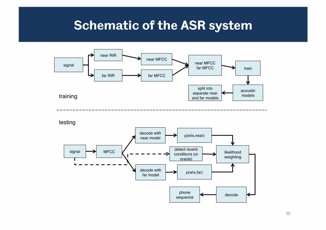
Schematic of the ASR system

10

signal" MFCC"

decode with near model"

decode with far model"

signal"

near RIR"

far RIR"

near MFCC"

far MFCC"

near MFCC"far MFCC" train"

acoustic models"

detect reverb conditions (or

oracle)"

p(w|x,near)"

p(w|x,far)"

likelihood weighting"

decode"phone sequence"

training"

testing"

split into separate near and far models"

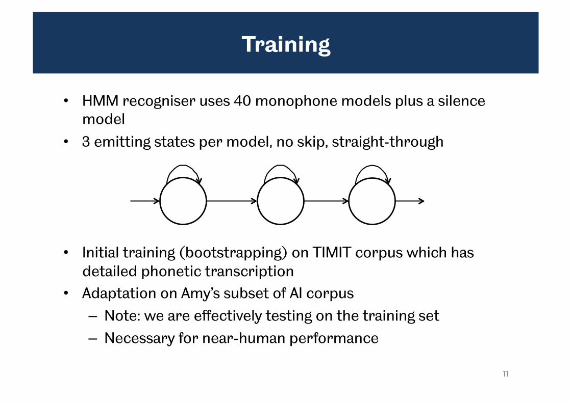
Training

•  HMM recogniser uses 40 monophone models plus a silence model

•  3 emitting states per model, no skip, straight-through

•  Initial training (bootstrapping) on TIMIT corpus which has detailed phonetic transcription

•  Adaptation on Amy’s subset of AI corpus –  Note: we are effectively testing on the training set –  Necessary for near-human performance

11

Acoustic features and training

•  12 MFCC features + deltas + accelerations

•  To avoid mismatch with Amy’s test stimuli, all training utterances were:

–  lowpass filtered to 4 kHz cutoff

–  had headphone correction filter applied

•  Training done by concatenating 2 x blocks of 36 features

–  one filtered with ‘near’ RIR

–  one filtered with ‘far’ RIR

•  Models split after training (done this way so that both models have the same segmentation during training)

12

MFCC features for one training utterance

13

MFCC features for ‘far’ reverberated signal

MFCC features for ‘near’ reverberated signal

Testing

•  Amy’s stimuli presented to the system during testing

•  MFCC features computed for the input signal and duplicated to form two feature streams

–  one set used as input to ‘near’ model

–  one set used as input to ‘far’ model

•  Effectively running two recognisers in parallel, and combining the observation state likelihoods

•  Used semi-forced alignment: ASR systems knows the context words and is only required to identify the test word

14

Combining feature streams in decoding

•  During recognition, for each feature frame x(t) at time t, the observation state likelihoods are computed from the HMMs for both feature streams

–  likelihood of a HMM state having generated the corresponding input feature frame x(t)

–  p(x(t)|λn) for the ‘near’ acoustic model

–  p(x(t)|λf) for the ‘far’ acoustic model

•  Combined near-far observation state likelihood is a weighted sum of likelihoods in the log domain

log[p(x(t)|λn,f)] = α(t) log[p(x(t)|λn)] + (1-α(t)) log[p(x(t)|λf)]

15

Determining the weighting factor α(t)

•  The weighting factor is adjusted dynamically according to the prevailing acoustic conditions

–  Low value of α(t) if reverberant environment

–  High value of α(t) if dry environment

•  Three schemes investigated here:

–  Use an ‘oracle’ value of α(t), assuming that context reverberation condition is know

–  Adjust α(t) according to the mean-to-peak ratio of the context speech envelope

–  Adjust α(t) according to maximum likelihood estimates from the near and far acoustic models

16

Evaluation metrics

•  Model performance expressed in terms of –  Percentage error in identifying test words –  1-RIT

•  Relative information transmitted (RIT) is an information-theoretic metric that reflects the distribution of errors in the confusion matrix:

RIT = H(X:Y)/H(X) •  H(X:Y) is the average mutual information of the input X and

output Y, and H(X) is the average self-information (entropy) of the input

•  Also compare human/machine confusions

17

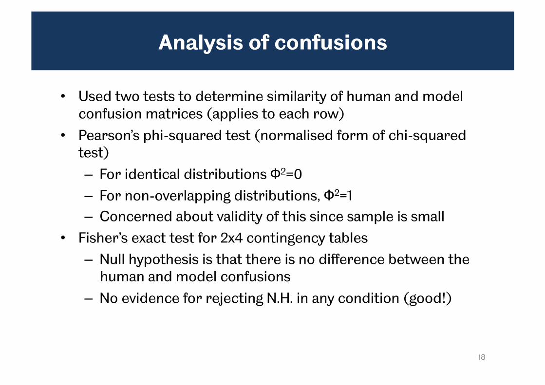
Analysis of confusions

•  Used two tests to determine similarity of human and model confusion matrices (applies to each row)

•  Pearson’s phi-squared test (normalised form of chi-squared test) –  For identical distributions Φ2=0 –  For non-overlapping distributions, Φ2=1 –  Concerned about validity of this since sample is small

•  Fisher’s exact test for 2x4 contingency tables –  Null hypothesis is that there is no difference between the

human and model confusions –  No evidence for rejecting N.H. in any condition (good!)

18

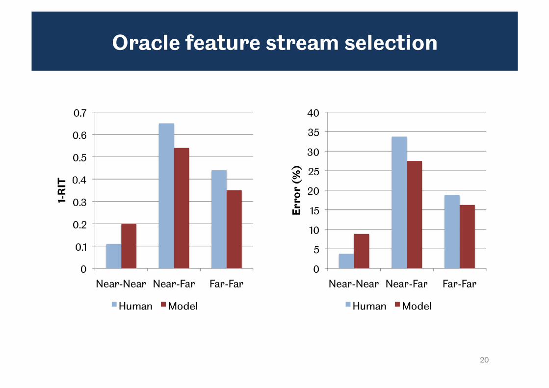
Oracle feature stream selection

•  In this condition we adjust the weighting α(t) based on a priori (‘oracle’) knowledge of the context reverberation condition

–  ‘near’ set α(t) = 1

–  ‘far’ set α(t) = 0

•  Gives an upper limit on model performance

–  No error in classification of the reverberation environment

•  Simple idea

–  if the reverberation condition of the context and target word are different, the acoustic model is mismatched and performance will fall

19

Oracle feature stream selection

20

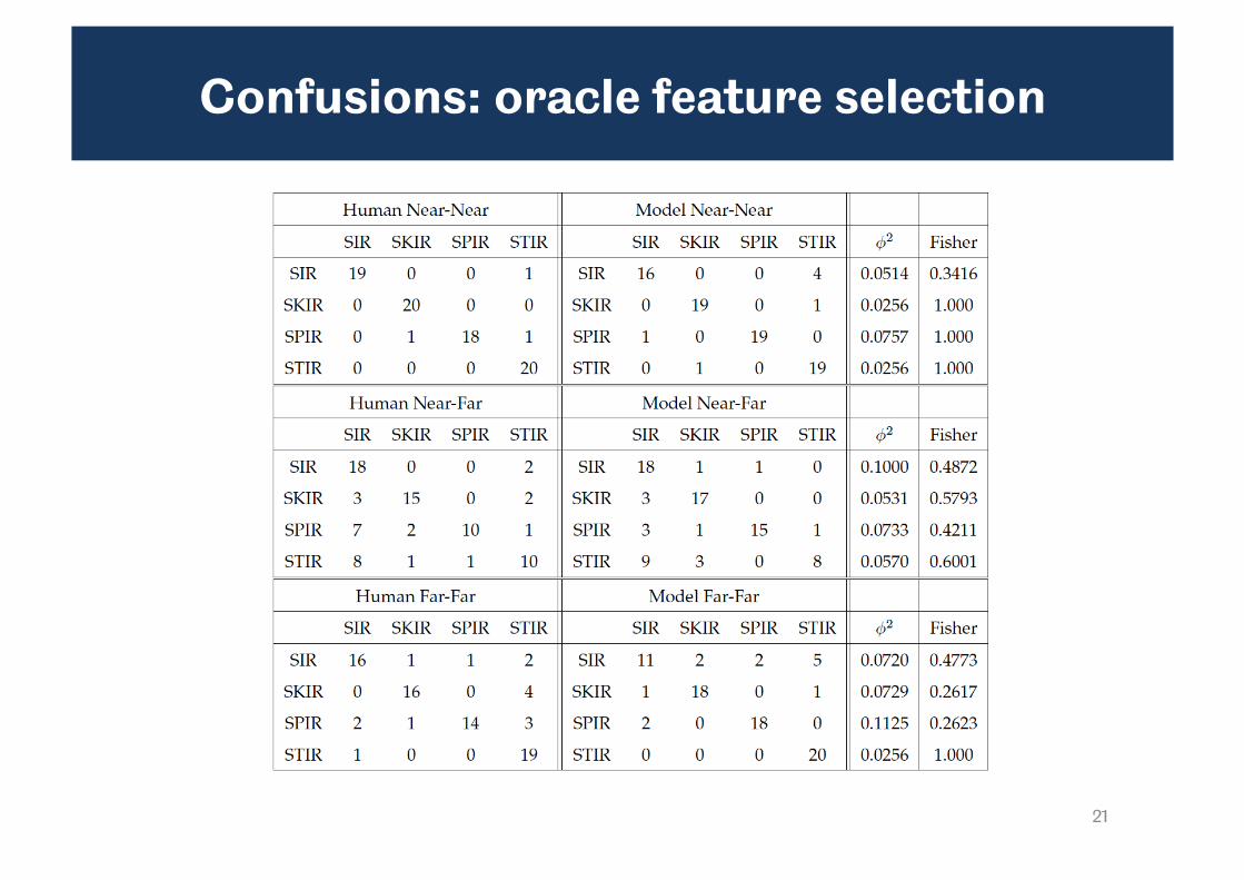
Confusions: oracle feature selection

21

Interim discussion

•  Overall model performance is similar to human listeners

–  Model error rate is higher than humans in the near-near condition, but lower in the other conditions

–  Similar results in terms of 1-RIT and percent error

•  Pattern of confusions made by the model is plausible

–  In near-far condition, predominant confusion is STIR SIR but also SPIR SIR and SKIR SIR

–  These confusions are resolved in the far-far condition

–  Fisher test indicates no difference between the distributions of model and listener responses for all test words

22

Feature selection by MPR

•  The ‘oracle’ model requires prior information about the reverberation condition of the context

•  In general, must estimate the reverberation condition from the signal

•  Use the mean-to-peak ratio of context envelope as a measure of reverberation present, as in Amy’s model

•  Gaussian classifier used to detect near/far condition •  Currently working across all frequency bands (see later)

23

MPR estimated in window model selection

Feature selection by MPR

•  The mean-to-peak ratio of the context speech envelope is computed from the Hilbert envelope

•  Here T is 500 ms •  Gaussian classifier trained on MPR to distinguish between

‘near’ and ‘far’ conditions. Compute the log odds:

•  If the context speech classified as ‘near’, otherwise ‘far’ •  83% correct classification on test set

24

€

MPR =1T

e(t)1

T∑ max

t[e(t)]

€

d = −12

*(MPR −µn)2

σn2 −

(MPR −µf )2

σ f2 + logσn

2 − logσ f2

⎡

⎣ ⎢

⎤

⎦ ⎥

€

d ≥ 0

Feature stream selection by MPR

25

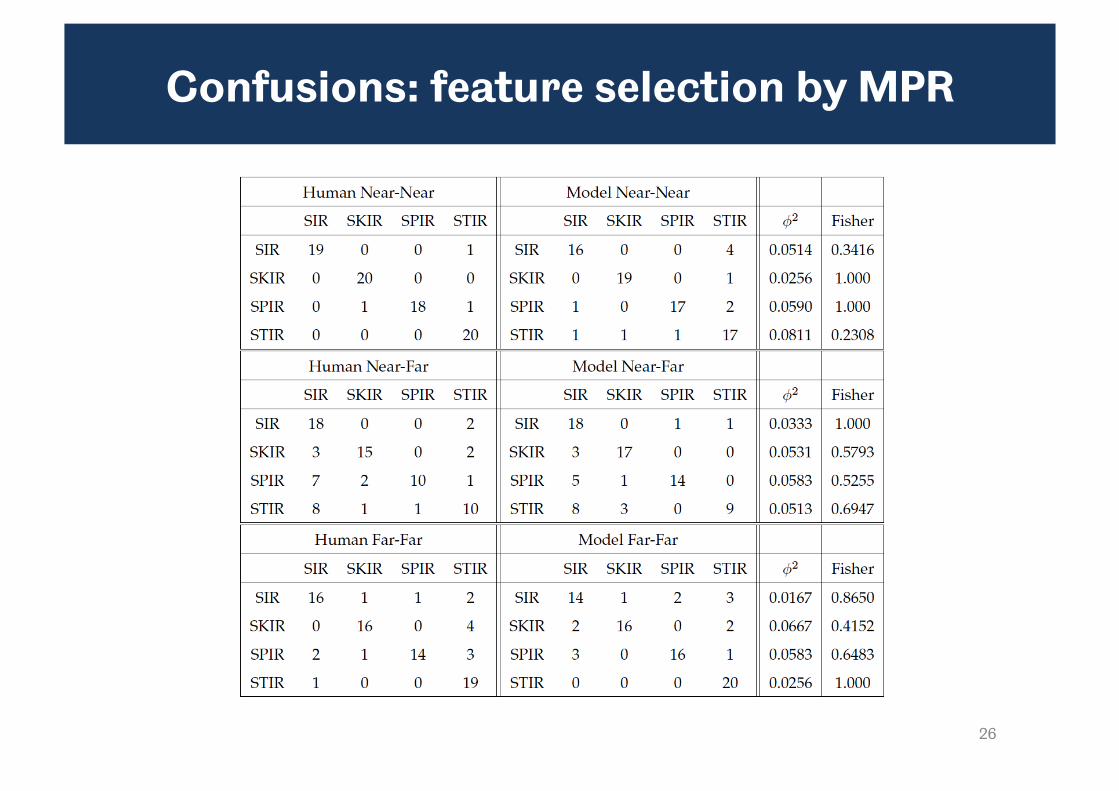
Confusions: feature selection by MPR

26

Interim discussion

•  Fully autonomous system still shows the right overall pattern

–  Constancy effect

–  Plausible pattern of confusions

•  However, note that overall error rate is higher (due to occasionaly misclassification of the context)

27

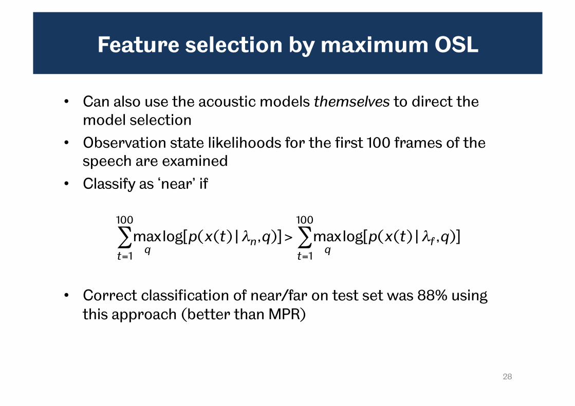
Feature selection by maximum OSL

•  Can also use the acoustic models themselves to direct the model selection

•  Observation state likelihoods for the first 100 frames of the speech are examined

•  Classify as ‘near’ if

•  Correct classification of near/far on test set was 88% using this approach (better than MPR)

28

€

maxqt=1

100

∑ log[p(x(t)|λn,q)] > maxqt=1

100

∑ log[p(x(t)|λf ,q)]

Matching ‘near’ and non-matching ‘far’

29

Observation state likelihoods

Maximum log likelihood across all states

Near model (matches) Far model (mismatched)

Feature stream selection by MOSL

30

Confusions: feature selection by MOSL

31

Interim discussion

•  Similar performance to the MPR version of the model

–  But error is higher in far-far condition, which somewhat reduces the magnitude of the compensation effect

–  Less impressive match to confusions in far-far condition (but still acceptable, and no statistically significant different from human confusion pattern)

32

Conclusions

•  All versions of the model

–  Exhibit a constancy effect in the same manner as the listeners in Amy’s experiment

–  Provide a good match to the pattern of consonant confusions made by listeners

33

Planned work for next period

•  A further extension of the model is to perform feature selection and combination on a band-by-band basis

–  Divide the features into, say, 8 bands

–  Train ‘near’ and ‘far’ HMMs for each band

–  During decoding, have a dynamic weight α(t,b) which is determined by reverberation estimate in band b

•  Could allow modelling of Tony’s experiments using noise-vocoded speech

•  Probably necessary to do this with spectral, rather than cepstral, features

34

Comments?

35