A Methodology and a Software Tool for Sensor Data

A Methodology and a Software Tool for Sensor DataValidation/Reconstruction: Application to the Catalonia Regional

Water Network

Miquel A. Cuguero-Escofeta, Diego Garcıaa, Joseba Quevedoa, Vicenc Puiga, SantiagoEspinb, Jaume Roquetb

aSupervision, Safety and Automatic Control Research Center (CS2AC), Polytechnic University of Catalonia (UPC), Terrassa Campus, GaiaResearch Bldg. Rambla Sant Nebridi, 22. 08222 Terrassa, Barcelona, Spain (e-mail:{miquel.angel.cuguero,diego.garcia,joseba.quevedo,vicenc.puig}@upc.edu).

bATLL Concessionaria de la Generalitat de Catalunya, SA. Sant Martı de l’Erm, 30. 08970 Sant Joan Despı, Barcelona, Spain (e-mail: {sespin,jroquet}@atll.cat).

Abstract

In this paper, a sensor data validation/reconstruction methodology applicable to water networks and its implementation by meansof a software tool, are presented. The aim is to guarantee that the sensor data are reliable and complete in case that sensor faultsoccur. The availability of such dataset is of paramount importance in order to successfully use the sensor data for further taskse.g. water billing, network efficiency assessment, leak localisation and real-time operational control. The methodology presentedhere is based on a sequence of tests and on the combined use of spatial models (SM) and time series models (TSM) applied to thesensors used for real-time monitoring and control of the water network. Spatial models take advantage of the physical relationsbetween different system variables (e.g. flow and level sensors in hydraulic systems) while time series models take advantageof the temporal redundancy of the measured variables (here by means of a Holt-Winters (HW) time series model). First, the datavalidation approach, based on several tests of different complexity, is described to detect potential invalid or missing data. Then, thereconstruction process is based on a set of spatial and time series models used to reconstruct the missing/invalid data with the modelestimation providing the best fit. A software tool implementing the proposed data validation and reconstruction methodology isalso described. Finally, results obtained applying the proposed methodology to a real case study based on the Catalonia regionalwater network is used to illustrate its performance.

Keywords: Sensor Data Validation/Reconstruction, Fault Isolation, Model-Based Fault Diagnosis, Time Series

1. Introduction

Critical Infrastructure Systems (CIS), including water, gas or electricity networks, are complex large-scale systemsgeographically distributed and decentralized with a hierarchical structure. These systems require highly sophisticatedsupervisory and real-time control schemes, to ensure high performance achievement and maintenance when conditionsare non-favourable [1, 2] due to e.g. sensor and actuator malfunctions (faults). Regarding the measurements in watersystems, the commonly measured hydraulic and quality variables include water flow rate in links, pressure in nodes,water level in tanks, pH, conductivity and turbidity, as well as disinfectant and pollutant concentrations. For eachmeasurement obtained from a sensor, the data (signals) are usually represented in the form of one dimensional time

1

2

series. Each sensor measures a physical quantity and converts it into a signal that can be read by the appropriateinstrumentation. Then, the measuring system converts the sensor signals into values aiming to represent a certainreal physical quantity. These values, known as raw data, need to be validated before further use in order to assurethe reliability of the results derived from their usage. In systems like CIS, a telecontrol system is acquiring, storingand validating data gathered from different kind of sensors every given sampling time (e.g. every few minutes) toaccurately real-time monitor the whole system. In the data acquisition process, several problems can occur, as thoserelated with the communication system (e.g. between sensors and data loggers or in the telecontrol system itself) oroutliers, producing lost or corrupted data which may be of great concern in order to have valid historic records. Whenthis is occurring, lost data should be replaced by a set of estimated data which should be representative of the data lost,since missing data may severely jeopardise further processes needing complete datasets in order to get meaningfulconclusions/analysis. Another common problem in CIS is caused by the unreliable sensors, which may be affectedby faults e.g. offset, drift, freezing in the measurements [3, 4, 5]. These unreliable data should also be detectedand replaced by forecasted data, since it may be used for system management tasks e.g. maintenance, planning,investment plans, billing, security and operational control [6] and system fault detection and isolation (Figure 1).In the case of water network applications, this system fault diagnosis may include e.g. network leaks isolation, asconsidered in [7, 8, 9]. However, the methodology presented here may well be applied to different applicationsinvolving a telemeasured sensor network, such as smart buildings or environmental systems (see, e.g. [10, 11]). Inaddition to the possible measurement deviations related to the sensor performance itself, the errors can also occurdue to heterogeneous reasons, e.g. sensor installation, calibration or electrical problems. Thus, it is important toprovide the data system with procedures that can detect these problems and assist the user in the monitoring andthe processing of the incoming data. The data validation is an essential step to improve data reliability. Sensordata validation and reconciliation have been intensively addressed using least-squares approaches including Kalmanfilters (see, e.g. [12, 13]). These have been also used for data forecasting, as pointed out in [14], where a review oftechniques for prediction of consumption in water and natural gas grids is presented. The basic idea of Kalman filterbased methods in data validation and reconciliation is to allow gross error detection and to provide reconstructed datathat is consistent with model/balance equations describing the system operation. The approach presented in this paperaims to assess the validity of each single sensor measurement by means of a set of tests exploiting not only the modelequations (spatial redundancy) but also temporal redundancy, using time series models and a bank of low-level tests(non-model based) aiming to label the data with a certain quality index. Traditionally, data validation process has beendeveloped by manual data analysis, performed by experienced users with the only assistance of basic data analysis andvisualisation tools [15], which significantly limits the amount of data to be validated [16] and the abnormal situationswhich may be correctly detected [17]. However, the volume of real data acquired in CIS is dramatically increasingdue to the increment of automated measurement systems allowing their monitoring [18]. Also, real-time operation,paramount in many real applications, makes human data validation even harder to pursuit. In order to cope with thissituation and increase the reliability of the data diagnosis system, automatic data validation tools have arised e.g.NIKLAS for real and non-real time diagnosis of meteorological data [19]. Also, in [20] a data validation module isconsidered in the framework of an on-line water quality fault tolerant control system. Over the last 15 years, moreand more affordable on-line sensors have become available, leading to ever increasing acceptance of on-line watermonitoring [21]. These on-line systems allow to deploy control mechanisms that are optimized for and respond to theactual process conditions. However, on-line systems require a data validation method that is applicable to real-timeincoming data. The major difference between on-line and off-line data validation lies in the available informationand the required execution time. In contrast with the on-line execution, the off-line operation has no time restrictionsbecause real-time constraints do not apply, and regarding the information, the whole set of data is available. Moreover,on-line data validation is usually required by a further real-time control system and thus the data are used for decisionsupport (or decision making) just after being obtained. Consequently, the on-line data validation process should havelow execution time, whereas the off-line data validation does not have this requirement.

According to the nature of the available knowledge, different kinds of data validation approaches may be con-sidered, with varying degrees of sophistication. In general, one may distinguish between elementary signal-based(“low-level”) methods and model-based (“high-level”) methods (see, e.g. [6]). Elementary signal based methods usesimple heuristics and limited statistical information of a given sensor [22]. Typically, these methods are based on vali-dating either signal values or signal variations. On the one hand, in the signal value-based approach, data are assessedas valid or invalid according to two different thresholds (high and low) so data are assumed to be invalid when lying

2

3

outside these threshold values. On the other hand, methods based on signal variations look for high variations (peaksin the curve) and low variations (flat curve) in the signals. Model-based methods rely on the use of models to check theconsistency of sensor data [21]. This consistency check is based on computing the difference between the predictedvalue from the model and the real value measured by the sensors. Then, this difference (known as residual) is com-pared with a threshold value (zero in the ideal case). When the residual is bigger than the corresponding threshold,a fault is assumed in the sensor; otherwise, the sensor is assumed to work properly. Moreover, the information of allthe available residuals and models allows performing fault isolation in order to discover the faulty sensor. Models areusually derived using either multivariate procedures exploiting the correlation or analytical relations between severalvariables, sometimes measured at different times (“temporal redundancy”) and/or locations (“spatial redundancy”).

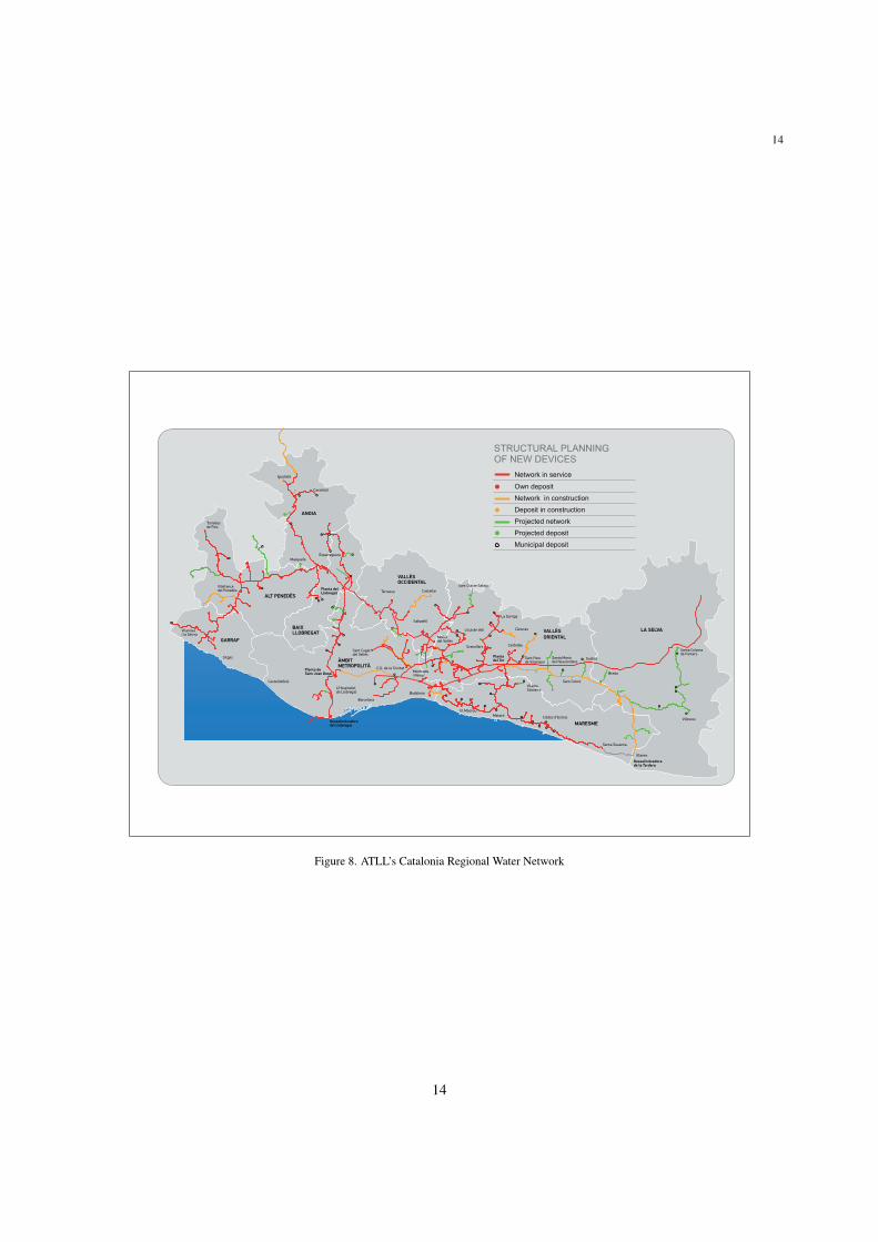
In this paper, a methodology is developed for validation and reconstruction of sensors data in a water network,taking into account not only spatial models (SM) but also time series models (TSM) for each flow and level meterhere. Also, internal models of every component in the local equipment units (e.g. pumps, valves, flows, levels)are considered. SM take advantage of the relation between different variables in the system (e.g. demand, pumpflows and tank levels) while TSM take advantage of the temporal redundancy of the measured variables, by meansof Holt-Winters (HW) time series models [23]. Moreover, after the corrupted sensor data are detected, they mustbe replaced by adequate estimated data using the available temporal/spatial redundancy. The methodology is mainlyapplied to flow and level meters, since it exploits the temporal redundancy of flow and level data in a water network.In this paper, an operative software tool implementing the presented methodology which is able to properly handleraw sensor data (including storage, querying and visualization) is also presented. The proposed approach and tool areapplied to several subsystems in the Catalonia regional water network (Figure 8) using raw data collected from ATLLConcessionaria de la Generalitat de Catalunya, SA (ATLL), the company managing this water network.

The structure of the paper is as follows: In Sections 2 and 3, the methodology to validate/reconstruct the sensordata, in order to provide a reliable dataset when faulty situations occur within the sensor set, is proposed. In Section 4,the software tool implementing the proposed methodology is introduced. In Section 5, the application case study ispresented, based on the Catalonia regional water network. The sensors in this network measure several real magnitudesof interest such demand and input tank flows and levels, considering real-world scenarios. Also, the correspondingresults obtained applying the proposed methodology are detailed in Section 5. Finally, conclusions of this work areoutlined in Section 6.

2. Proposed Methodology

2.1. DescriptionIn real water networks such as the one considered here, there is usually a telemeasurement system acquiring,

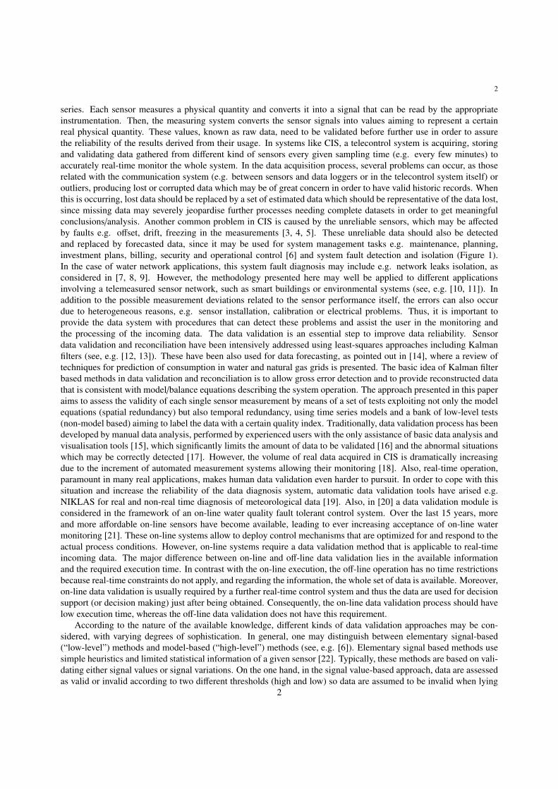
recording and validating data gathered from different kind of sensors at each sample time to accurately real-timemonitor the whole network [6]. As discussed in the introduction, in this data acquisition process, problems in thecommunication system (e.g. between sensors and data loggers) or in the telemeasurement system itself (e.g. sensorsmay be affected by e.g. offset, drift or freezing faults), often arise and produce data loss, which may be of greatconcern in order to have valid historic records. These unreliable data should be detected and replaced by estimateddata before they can be used for system management tasks such as maintenance, planning, billing and operationalcontrol, as depicted in the procedure in Figure 1. The input to this procedure is the raw data yraw gathered fromthe sensors. The process is divided in two different stages: the first stage is related with the data validation, whilethe second stage addresses the reconstruction of invalid/missing data, before the data are stored in an operationaldatabase (DB) for further use. At the first stage (data validation, detailed in Figure 2), if the datum yraw(k) at a certainsample time k is validated, flag v is set to 1 and datum yval(k) = yraw(k) is stored in the aforementioned operationalDB as validated data. Conversely, if the datum yraw(k) is invalidated, flag v is set to 0 and the datum reconstructionprocess (second stage) is started, in order to provide a reconstructed estimation yrec(k) of the invalid/missing datayraw(k) to be stored in the DB. The whole procedure is further detailed in Algorithm 1 for the data validation stageand in Algorithm 2 for the data reconstruction stage. Here, communication and sensor faults are considered as faultsaffecting the telemeasurement system and the sensors, respectively, and the data detection/reconstruction procedure isused as a prefilter to estimate the invalid/missing data when these type of faults are occurring.

As discussed in the introduction, different types of data detection methods with distinct degrees of complexity maybe considered according to the available system knowledge. This is the approach that the proposed methodology here

3

4

Data

ValidationValidated?

Data

Reconstruction

No

Operational

DataBaseYes

Raw sensor

data

( )rawy k( ) 1v k =

( ) 0v k =

( )valy k

( )recy k

Figure 1. Raw data validation/reconstruction procedure

will follow. Generally, two types of methods are considered, one for elementary ‘low-level’ signal-based methods andanother for ‘high-level’ model-based methods. The first type uses simple heuristics and limited statistical informationfrom the sensors [22] [15] and is typically based on checking either signal values or variations, whilst the second typeuses models for consistency-checking of the sensor data [21].

2.2. Validation Tests

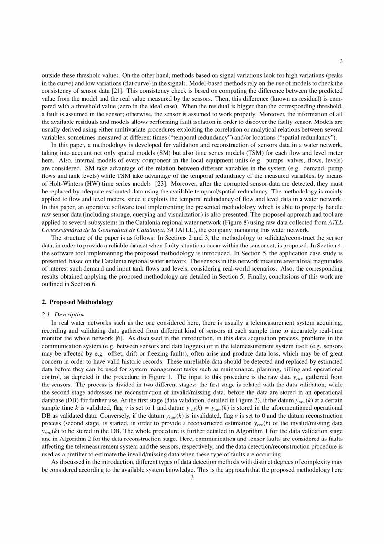
The data detection process presented is inspired by the Spanish AENOR-UNE norm 500540 developed for datavalidation in meteorological stations [6]. The methodology presented here applies a set of consecutive detection teststo a given dataset (Figure 2), to finally assign a certain quality level q depending on the number of tests passed. Also,the corresponding tests passed are characterized by a validation vector l, as shown in Figure 2. If the datum yraw(k) ata certain sample time k is voided at any validation level, flag v is set to 0 and the datum reconstruction process (secondstage) is started. Conversely, if the datum yraw(k) pass all the validation levels, flag v is set to 1 and the data arevalidated (i.e. yval(k) = yraw(k)). In the latter situation i.e. validated datum yraw(k), q(k) = 6 and l(k) = [1, 1, 1, 1, 1, 1].

The validation tests include a set of ’low-level’ tests (Levels 0 to 3, included) which check elementary signal prop-erties, and a set of ’high-level’ tests (Level 4 and Level 5), which rely on the use of models to check the consistencyof the sensor data. The latter models are also used in the reconstruction stage of the potentially invalidated data, asexplained in Section 3.3. As introduced in the last paragraph, if any of the validation tests in Figure 2 is not satisfied,v = 0. The validation procedure is also detailed in Algorithm 1.

Level 0

Communications

Level 1

Physical range

Raw sensor

data

Level 2

Trend

Level 3

Equipment State

Level 4

Spatial Consistency

Level 5

Time Series Consistency

( )

( ) 0

( ) 1

rawy k

q k

v k

=

=

( )v k

Passed?

Yes

No

0 ( ) 1

( ) ( ) 1

l k

q k q k

=

= +

0 ( ) 0

( ) 0

l k

v k

=

=

Passed?

Yes

No

1( ) 1

( ) ( ) 1

l k

q k q k

=

= +

1( ) 0

( ) 0

l k

v k

=

=Passed?

Yes

No

2 ( ) 1

( ) ( ) 1

l k

q k q k

=

= +

2 ( ) 0

( ) 0

l k

v k

=

=Passed?

Yes

No3( ) 0

( ) 0

l k

v k

=

=

Passed? No4 ( ) 0

( ) 0

l k

v k

=

=

Yes

4

( ) ( ) 1

( ) 1

q k q k

l k

= +

=

Passed? No5 ( ) 0

( ) 0

l k

v k

=

=

Yes

5

( ) ( ) 1

( ) 1

q k q k

l k

= +

=

( )kl

( )q k

3( ) 1

( ) ( ) 1

l k

q k q k

=

= +

Figure 2. Data Validation Tests

An explanation of the test applied to each level is given next:

4

5

• Level 0: This level, also called communications level, checks whether the data are properly recorded at a regularsample rate by the acquisition system. If this is not fulfilled, there is some communication problem involvinge.g. the data transmission from the ground sensors to the operational database. Hence, this level allows detectingproblems in the data acquisition or communication system, which is one of the most common faults affectingtelemeasurement systems, as the one considered here.

• Level 1: This level, also called physical range level, checks whether the data are within the physical range ofthe sensor acquiring the corresponding measurement. The expected range of the measurements may be obtainedfrom e.g. sensor specifications or historical records of the data.

• Level 2: This level, also called trend level, checks whether the data derivative i.e. the magnitude change ofthe data among consecutive sample times, are within their expected rate. This allows detecting unexpected andpossibly undesired sudden changes in the data, e.g. in a water network, tank water level sensors measurementscannot change more than several centimeters per minute.

• Level 3: This level, also called equipment state level, allows to check the consistency of the variables in a givenequipment unit i.e. sensor or actuator. For example, in a water network system, in a pipe with a valve and aflow meter installed, there is a relation between the valve state and the flow meter reading.

• Level 4: This level, also called spatial consistency level, checks the consistency of the data collected by acertain sensor with its SM [24], i.e. the correlation between data coming from spatially-related sensors. ThisSM is obtained from the physical relations among these variables. In hydraulic systems, this relation is generallyobtained from the mass balance model of the element relating the different measured variables involved.

• Level 5: This level, also called time series consistency level, checks for temporal consistency of a given sensormeasurement, by means of a TSM obtained from sensor historical records under faultless assumption ([6]). Acommon method for time series signal forecasting is the HW approach ([23], [25]) because of its simplicity andlow computational and storage requirements. In contrast to spatial consistency level, time series consistencylevel only uses information of the considered sensor without needing additional information (e.g. networktopology or extra measurements from the system) to perform the validation, which makes it convenient whenthere is no such additional information available or the sensors needed by the corresponding spatial consistencylevel are unreliable. At this level, the analysis of the historic measurement records of a certain sensor are usedto obtain the corresponding HW TSM sensor model and to validate the current data acquired by this element.

3. Model-based Data Validation/Reconstruction Levels

3.1. Models for Data Validation/Reconstruction

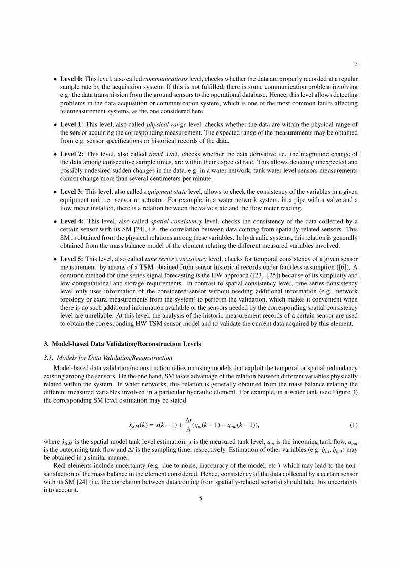
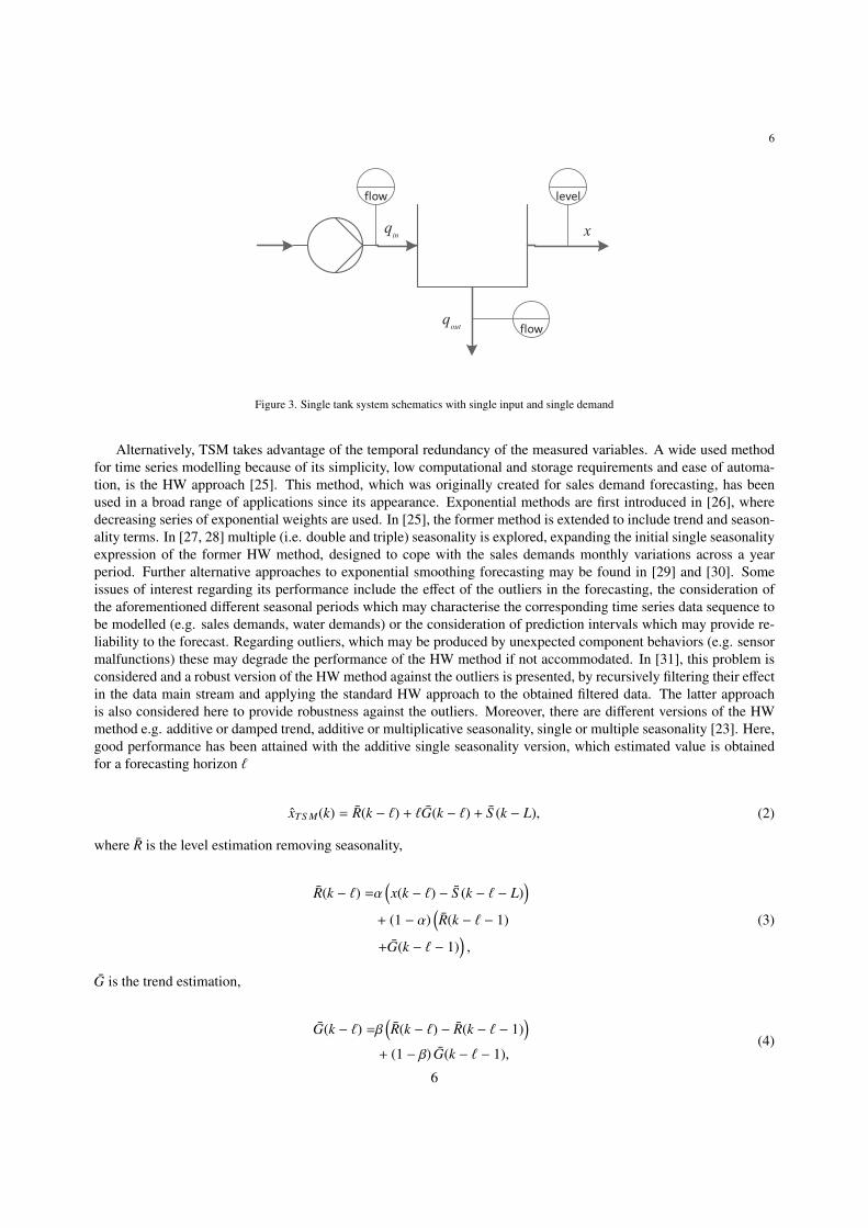
Model-based data validation/reconstruction relies on using models that exploit the temporal or spatial redundancyexisting among the sensors. On the one hand, SM takes advantage of the relation between different variables physicallyrelated within the system. In water networks, this relation is generally obtained from the mass balance relating thedifferent measured variables involved in a particular hydraulic element. For example, in a water tank (see Figure 3)the corresponding SM level estimation may be stated

xS M(k) = x(k − 1) +∆tA

(qin(k − 1) − qout(k − 1)), (1)

where xS M is the spatial model tank level estimation, x is the measured tank level, qin is the incoming tank flow, qout

is the outcoming tank flow and ∆t is the sampling time, respectively. Estimation of other variables (e.g. qin, qout) maybe obtained in a similar manner.

Real elements include uncertainty (e.g. due to noise, inaccuracy of the model, etc.) which may lead to the non-satisfaction of the mass balance in the element considered. Hence, consistency of the data collected by a certain sensorwith its SM [24] (i.e. the correlation between data coming from spatially-related sensors) should take this uncertaintyinto account.

5

6

flow level

flow

inq

outq

x

Figure 3. Single tank system schematics with single input and single demand

Alternatively, TSM takes advantage of the temporal redundancy of the measured variables. A wide used methodfor time series modelling because of its simplicity, low computational and storage requirements and ease of automa-tion, is the HW approach [25]. This method, which was originally created for sales demand forecasting, has beenused in a broad range of applications since its appearance. Exponential methods are first introduced in [26], wheredecreasing series of exponential weights are used. In [25], the former method is extended to include trend and season-ality terms. In [27, 28] multiple (i.e. double and triple) seasonality is explored, expanding the initial single seasonalityexpression of the former HW method, designed to cope with the sales demands monthly variations across a yearperiod. Further alternative approaches to exponential smoothing forecasting may be found in [29] and [30]. Someissues of interest regarding its performance include the effect of the outliers in the forecasting, the consideration ofthe aforementioned different seasonal periods which may characterise the corresponding time series data sequence tobe modelled (e.g. sales demands, water demands) or the consideration of prediction intervals which may provide re-liability to the forecast. Regarding outliers, which may be produced by unexpected component behaviors (e.g. sensormalfunctions) these may degrade the performance of the HW method if not accommodated. In [31], this problem isconsidered and a robust version of the HW method against the outliers is presented, by recursively filtering their effectin the data main stream and applying the standard HW approach to the obtained filtered data. The latter approachis also considered here to provide robustness against the outliers. Moreover, there are different versions of the HWmethod e.g. additive or damped trend, additive or multiplicative seasonality, single or multiple seasonality [23]. Here,good performance has been attained with the additive single seasonality version, which estimated value is obtainedfor a forecasting horizon `

xTS M(k) = R(k − `) + `G(k − `) + S (k − L), (2)

where R is the level estimation removing seasonality,

R(k − `) =α(x(k − `) − S (k − ` − L)

)+ (1 − α)

(R(k − ` − 1)

+G(k − ` − 1)),

(3)

G is the trend estimation,

G(k − `) =β(R(k − `) − R(k − ` − 1)

)+ (1 − β) G(k − ` − 1),

(4)

6

7S¯is the seasonal component estimation,

S (k − `) =γ(x(k − `) − R(k − `)

)+ (1 − γ) S (k − ` − L),

(5)

and L is the season (daily) periodicity, α, β and γ are the HW parameters (level, trend and season smoothing factors,respectively), x is the measured value and xTS M is the TSM estimated value. The parameters α, β and γ are in theinterval [0, 1] and can be estimated from historical data using the least-squares approach. Hence, analysing the historicrecords of a certain sensor, a HW TSM model can be obtained and used to estimate missing data of this element whena fault is affecting its readings.

3.2. Data Validation

On the one hand, the test check for the so-called ’low-level’ tests are straightforward, since they rely on basicsignal-based heuristics. On the other hand, the ’high-level’ model-based tests rely on checking for consistency bymeans of the residuals ri(k), obtained from the difference between the system measurements and the correspondingSM or TSM estimations, expressed in input-output regressor form

ri(k) = xi(k) − xi(k) = xi(k) − φTi (k)θi, (6)

where θi are the nominal parameters obtained using a training dataset, xi is the sensor measurement, xi is the modelprediction and φi(k) is the regressor vector of dimensions nθi × 1 including inputs (ui(k), ui(k − 1), ui(k − 2), ...) andoutputs (yi(k), yi(k−1), yi(k−2), ...). The particular models used to compute the prediction xi at instant k depend on thevalidation level considered (i.e. model-based level 4 or 5 in Figure 2, respectively), and are introduced in Section 3.3.Considering the uncertainty (e.g. modelling errors, noise), the detection test involves checking the condition

|ri(k)| < τi, (7)

where τi is the detection threshold. The detection threshold can be determined using statistical methods [32] or set-membership approaches [33]. In the case of statistical methods, the noise is assumed to follow a normal distributionwith known mean value µi and standard deviation σi [34]. Then, the threshold of the i-th residual can be determinedas follows: τi = µi + 3σi, including the 99.7 % of the values of a normal distribution according to the 3-sigma rule.Alternatively, when using a set-membership approach the noise is assumed to be unknown but bounded, with a prioriknown bound. Then, the threshold can be obtained by propagating the uncertainty to the residual computation [33].Using either one or the other approach, the threshold in (7) is determined to include the values of the whole residualdistribution in the faultless situation and hence, it may be used for fault detection purposes. This threshold is alsouseful to provide prediction interval bounds for the data forecasting process, so test condition (7) can be equivalentlyexpressed as follows

xi(k) ∈ [xi(k), ¯xi(k)], (8)

where ¯xi(k) = xi(k) + τi and xi(k) = xi(k) − τi, respectively. Condition (8) applies both to SM (1) and TSM (2)models. These interval bounds (8) consider the corresponding model behavior under faultless conditions includingthe uncertainty effect, as introduced in the residual bound condition (7). Hence, these bounds could alternatively beused in the data validation process, in order to decide whether a data sample at time instant k is reliable. The wholedata validation process is detailed in Algorithm 1.

7

8

3.3. Data Reconstruction

As introduced in Section 2, when a fault is detected at the validation stage and the corresponding data are voided,a reconstruction process is started until the sensor data are validated again. The output of the data validation process(Figure 1) is used to identify the invalidated data that should be reconstructed. SM, related with Level 4 in Figure 2,and TSM, related with Level 5 in Figure 2, are used for this purpose, depending on the performance of each model.This data reconstruction process is detailed in Algorithm 2. The performance of each model is measured by the MeanSquared Error (MSE), evaluated in a moving horizon window

MS E(k) =1m

k∑j=k−m

e( j)2, (9)

where m is the number of data samples considered in the window, e( j) = x( j) − x( j) is the error at instant j, x( j) isthe measured value at instant j, x( j) is the estimated value by the model (SM or TSM, respectively) at instant j andk is the actual time instant. The model having best MSE index before the fault occurs (i.e. when the data validationprocess is not satisfactory) is used to produce the reconstructed sensor signal.

In order to produce the forecasted signal, it is desirable to use measured data instead of estimated data, to avoidmodel uncertainty effects in the forecasted value. This calls for the computation of xi(k)|` using (2) with ` , 1 whenpossible and the usage of the different models obtained in a gain-scheduling fashion when e.g. the data are invalidatedfor more than a single time instant. HW TSM models may obtain forecasted values for different prediction horizons `by design, if forecasted value at time k in (2) is rewritten as follows

xTS M(k)|` = R(k) + `G(k) + S (k − L + `), (10)

Then, measured values may be used to produce the TSM forecasted signal within a complete season (day) Lwithout using old forecasted values. In order to achieve this, the complete set of models (i.e. the models for each stepwithin the complete season L) must be obtained at the calibration stage under faultless assumption, i.e. a HW TSMmodel [α`, β`, γ`] may be obtained for ` = 1, · · · , L.

Similar procedure may be used in the same case study for alternative applications not related with data valida-tion/reconstruction, as e.g. consumer demand prediction, in order to forecast water network user behavior beforehand.HW TSM models are specially suited to this end, since they were created in order to predict market product sales evo-lution according to consumer periodical behaviors [25], and user water consumption in district metered areas have asimilar behavior.

4. Software Framework

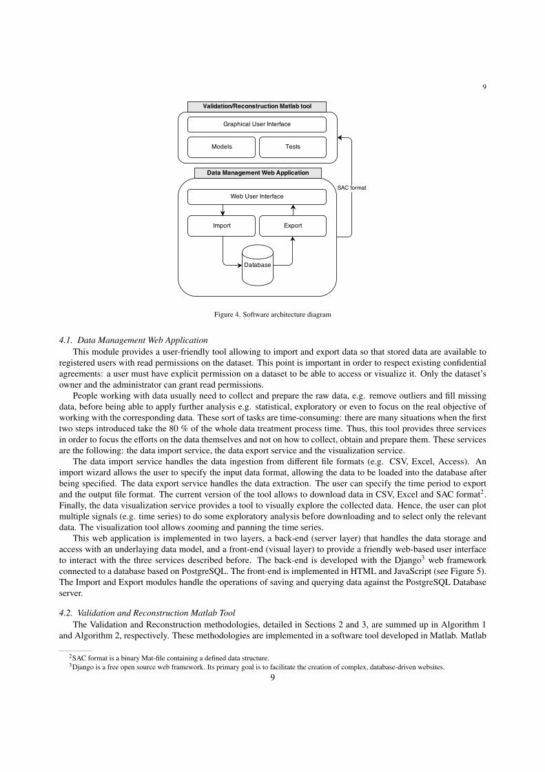
The architecture of the software framework implemented is depicted in Figure 4. There are two main components:the Data Management Web application and the Validation and Reconstruction tool1.

On the one hand, the Data Management component is a web application focused on collecting and serving timeseries data, i.e. observations coming from any kind of sensor. It allows authorized users to upload new data, downloadhistorical data and visualize data from anywhere using a device with a browser and Internet connection. Thus, thisweb-based data repository is highly available and provides a solution to the data-driven users to keep centralized datafrom different projects and sources. It also avoids typical datasets-usage related drawbacks e.g. data loss, sparse andduplicated data locations and emails with large datasets between project members.

On the other hand, the Validation and Reconstruction component allows users to apply the methodologies de-scribed in Sections 2 and 3 on data provided by the Data Management web application.

1Both software tools are proprietary software.

8

9

Figure 4. Software architecture diagram

4.1. Data Management Web ApplicationThis module provides a user-friendly tool allowing to import and export data so that stored data are available to

registered users with read permissions on the dataset. This point is important in order to respect existing confidentialagreements: a user must have explicit permission on a dataset to be able to access or visualize it. Only the dataset’sowner and the administrator can grant read permissions.

People working with data usually need to collect and prepare the raw data, e.g. remove outliers and fill missingdata, before being able to apply further analysis e.g. statistical, exploratory or even to focus on the real objective ofworking with the corresponding data. These sort of tasks are time-consuming: there are many situations when the firsttwo steps introduced take the 80 % of the whole data treatment process time. Thus, this tool provides three servicesin order to focus the efforts on the data themselves and not on how to collect, obtain and prepare them. These servicesare the following: the data import service, the data export service and the visualization service.

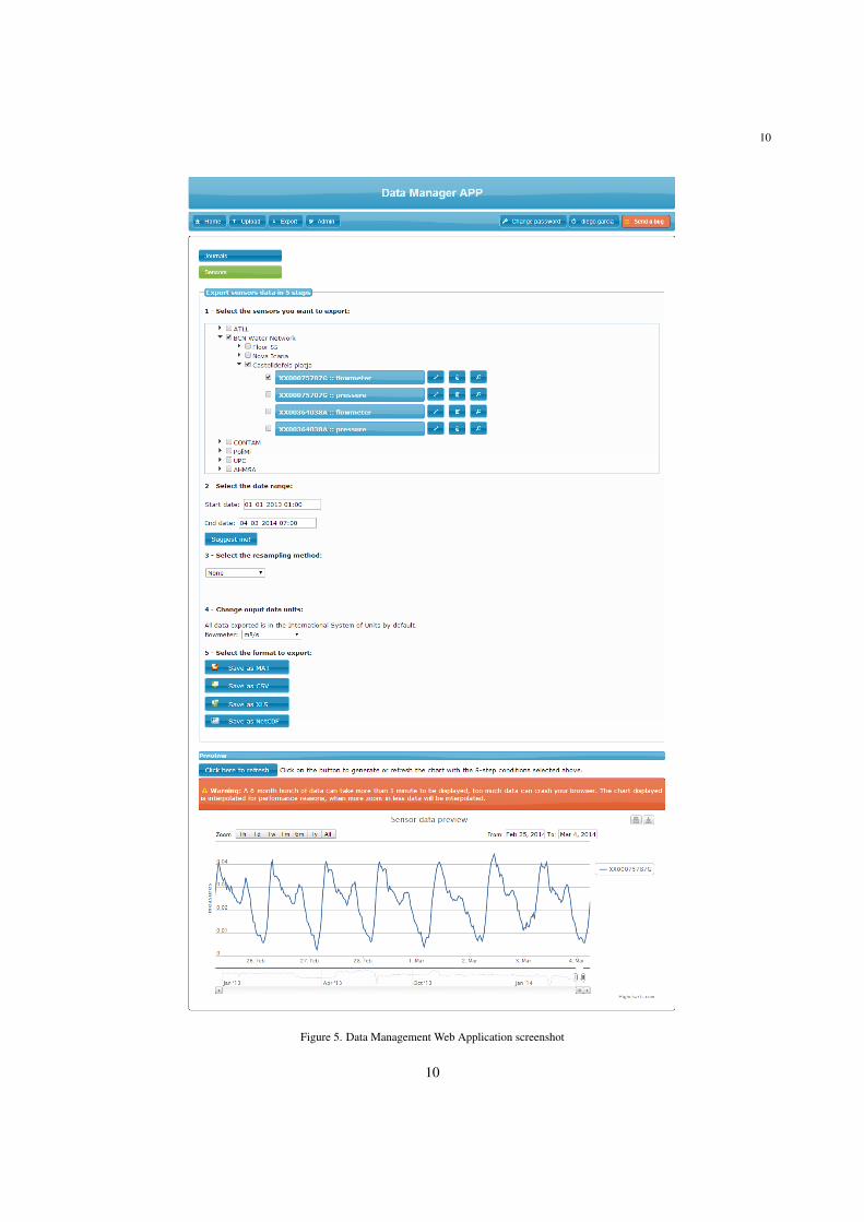
The data import service handles the data ingestion from different file formats (e.g. CSV, Excel, Access). Animport wizard allows the user to specify the input data format, allowing the data to be loaded into the database afterbeing specified. The data export service handles the data extraction. The user can specify the time period to exportand the output file format. The current version of the tool allows to download data in CSV, Excel and SAC format2.Finally, the data visualization service provides a tool to visually explore the collected data. Hence, the user can plotmultiple signals (e.g. time series) to do some exploratory analysis before downloading and to select only the relevantdata. The visualization tool allows zooming and panning the time series.

This web application is implemented in two layers, a back-end (server layer) that handles the data storage andaccess with an underlaying data model, and a front-end (visual layer) to provide a friendly web-based user interfaceto interact with the three services described before. The back-end is developed with the Django3 web frameworkconnected to a database based on PostgreSQL. The front-end is implemented in HTML and JavaScript (see Figure 5).The Import and Export modules handle the operations of saving and querying data against the PostgreSQL Databaseserver.

4.2. Validation and Reconstruction Matlab ToolThe Validation and Reconstruction methodologies, detailed in Sections 2 and 3, are summed up in Algorithm 1

and Algorithm 2, respectively. These methodologies are implemented in a software tool developed in Matlab. Matlab

2SAC format is a binary Mat-file containing a defined data structure.3Django is a free open source web framework. Its primary goal is to facilitate the creation of complex, database-driven websites.

9

10

Figure 5. Data Management Web Application screenshot

10

11

is a widely used numerical computing and programming platform in many research institutions and industrial enter-prises, which makes it a convenient prototyping and development framework. This tool includes a Graphical UserInterface (GUI) to configure different modules and to run the validation and reconstruction processes with the config-ured settings (Figure 6). This GUI is composed by six panels. Following the numeration in the figure, each panel hasthe following purpose:

1. Input data. The user can select the .mat file path in SAC format and load the data into the tool.2. Signals list. This panel shows the listing of the signals loaded in the previous panel.3. Fault generator. This module provides a fault generator framework in order to simulate different types of fault,

thus the user can apply a fault to the selected signals. The faults available are: freezing, offset, drift, noise andcommunication.

4. Data ranges. This panel allows the user to indicate the season periodicity L (cycle time) of the TSM. Forinstance, if a signal shows a daily pattern, the cycle time is 24 hours (86400 seconds). The user can also definethe number of identification and validation cycles. The rest of the data will be used as testing dataset.

5. Tests and Models. This panel lists the tests and the models available. Here, the user can select the tests to applyand configure the required parameters, depending on the models and tests selected.

6. Output and Reporting. In this panel, the user can enter the path where the results will be recorded and selectthe reporting options.

Algorithm 1 Data validationRequire: yraw(k)

v(k) = 1; # Initialise v(k)q(k) = 0; # Initialise q(k)for all Validation levels n = 0, · · · , 5 do

Check validation level test n;if Validation test n passed then

ln(k) = 1; # Set level n as passedq(k) = q(k) + 1; # Increase quality level of datum yraw(k)

elseln(k) = 0; # Set level n as not passedv(k) = 0; # Void datum yraw(k)

end ifend forif v(k) = 1 then

yval(k) = yraw(k); # Datum yraw(k) is validatedelse

yval(k) = []; # Datum yraw(k) is voidedend ifreturn v(k), l(k), q(k), yval(k)

The input dataset selected in the Input data panel (Figure 6) is divided in three different subsets (i.e. calibration,validation and testing) in order to calibrate and validate the models and parameters, and check the sensors’ raw data,respectively. The use of different data subsets allows the analysis and validation of how these models will generalize toan independent dataset. Calibration and validation subsets are assumed to be faultless, whilst testing dataset includesthe faulty scenario to be diagnosed. The different subset ranges are defined by the user according to the parametersentered in the Data ranges panel (Figure 6).

Once all the required parameters are set by the user the process may be started, which will sequentially apply thepresented methodology to the data. This process is divided in three different stages, namely Calibration, Validationand Reconstruction, respectively. First, the Calibration stage is executed using the calibration and validation datasetsin order to learn and estimate the parameters required by the tests and the models to be applied (see Sections 2 and3). Once the models and the tests are calibrated, the Validation stage runs the sequence of tests in order to validate the

11

12

Algorithm 2 Data reconstructionRequire: yraw(k), v(k)

if v(k) = 0 thenCompute MS ES M(k) and MS ETS M(k); # Evaluate MS E for each modelif MS ES M(k) < MS ETS M(k) then

yrec(k) = xS M(k); # Reconstructed datum yraw(k) is given by SM estimationelse

yrec(k) = xTS M(k); # Reconstructed datum yraw(k) is given by TSM estimationend if

elseyrec(k) = []; # If datum yraw(k) is validated, no reconstruction is needed

end ifreturn yrec(k)

Figure 6. Validation and Reconstruction Matlab Tool

12

13

testing dataset (see Section 2). Each test applied labels each datum yraw(k) with a flag (l in Figure 2 and Algorithm 1)to indicate whether the test has been fulfilled. Finally, in the Reconstruction stage (see Section 3.3), the model withbest performance (i.e. lowest MSE) is selected in order to replace the invalidated datum at the Validation stage (datumwith v = 0 in Figure 2 and Algorithm 1) by its corresponding reconstructed estimation. In Figure 7, the data flowbetween these three stages is presented.

Figure 7. Validation and Reconstruction data flow diagram

5. Case Study: Catalonia Regional Water Network

5.1. Description

The Catalonia regional water network managed by ATLL company (Figure 8) supplies water to the metropolitanarea of Barcelona. Most of the population of the region (approximately 4.5 million people) is concentrated in thisarea. This network transports the drinking water from the main water treatment plants (ETAPs), which take the waterfrom two different rivers (Llobregat and Ter), towards the main storing and buffer tanks of 116 different municipalitiesin the Barcelona metropolitan area, using about 1045 km of pipes of up to 3 m diameter. The network is composedby 170 storage tanks, 67 pumps and 212 demand sectors, and is monitored using more than 200 flow meters and 115tank level sensors by means of a SCADA system with 10 minutes sample time.

5.2. Results

In this section, some results obtained with the methodology introduced here are presented, using the tool intro-duced in Section 4. These results are based on a variety of real situations in order to show the performance of themethodology and the tool presented. The dataset used to obtain these results is the network’s raw data collected byATLL company, including flow meter measurements, level meter measurements, valve positions and communicationsystem alarms.

In Figure 9, the first fault scenario considered is shown. The top plot shows the measured signal (solid black line)gathered from the flow meter D6FT00204 CI, with a time range from 3rd to 8th of January 2014. On the one hand,the pattern of the measured signal for days 4th, 6th and 7th of January, respectively, present a similar behavior, witharound 300 m3/h peak. On the other hand, the pattern of the measured signal on January the 5th presents negativepumping flows, which should be corrected. This change in the pattern is detected by the physical range test (Level 1

13

14

GARRAF

BAIX LLOBREGAT

ANOIA

Igualada

Castellolí

VALLÈSOCCIDENTAL

VALLÈSORIENTAL

LA SELVA

MARESME

ÀMBIT METROPOLITÀ

ALT PENEDÈS

Vilafrancadel Penedès

Torrellesde Foix

Vilanovai la Geltrú

Sitges

Castelldefels

Planta deSant Joan Despí

Dessalinitzadora del Llobregat

L’Hospitaletde Llobregat

Barcelona

Badalona

Montcadai Reixac

E.D. de la Trinitat

Sant Cugatdel Vallès

Planta delLlobregat

Masquefa

Esparreguera

Terrassa Castellar

Sabadell

Sant Quirze Safaja

La Garriga

Lliçà de Vall

Granollers

Molletdel Vallès

Cànoves

Cardedeu

Sant Perede Vilamajor

Sant Celoni

Breda

Vidreres

Santa Colomade Farners

GualbaSanta Mariade Palautordera

VilalbaSasserra

Caldes d’Estrac

Santa Susanna

Blanes

Planta del Ter

El Masnou

Mataró

Dessalinitzadora de la Tordera

!"#$!#"%&'(&%))*)+'',-')./'0.1*$.

)234567'89':26;8<2

,49'=2>5:83

)234567''89'<59:36?<3859

02>5:83'89'<59:36?<3859

(65@2<32='9234567

(65@2<32='=2>5:83

A?98<8>BC'=2>5:83

Figure 8. ATLL’s Catalonia Regional Water Network

14

15

01/04 01/05 01/06 01/07 01/08

0

100

200

300

400

500m

³/h.

D6FT00204_CI

01/04 01/05 01/06 01/07 01/080

1

2x 10

4 MSE

MS

E

01/04 01/05 01/06 01/07 01/08

Valid

Invalid

Validation

measuredestimatedreconstructed valuespace coherencetime series

space coherencetime series

test limitstest derivativetime series

Figure 9. Results of the validation and reconstruction methodology, flow meter D6FT00204 CI

in Figure 2). The detection is indicated by the flags in the bottom plot in Figure 9: if the test flag is set to zero (Validstate) the datum pass the test; if it is set to one (Invalid state) the datum is invalidated. Using these flags, it maybe noted how negative flows are detected e.g. at the beginning of days 4th, 5th and 6th of January, although theirmagnitude are too low to make them visible in the top plot in Figure 9. The top plot in the latter figure also showsthe SM (dashed red line) and the HW TSM (dashed cyan line) estimations. The invalid observations are replaced byestimations (magenta dots) obtained from the model having the best performance according to their MSE (middle plotin Figure 9), as introduced in Section 3.3.

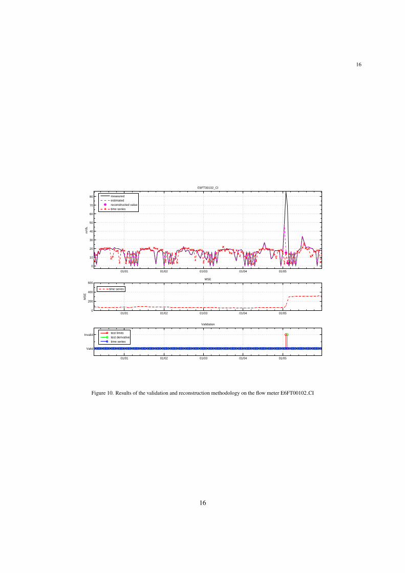
Figure 10 presents a different scenario, where the measured flow signal E6FT00102 CI exhibits a peak of highmagnitude on the fifth day of January 2014. In contrast to the previous scenario, in the current scenario there is onlythe TSM model available, since no SM model can be obtained due to the topological configuration of the network.However, validation and reconstruction can also be performed since TSM only needs historical records from the singlesensor under study to operate, i.e. does not need additional data gathered by other related sensors as is the case withSM models. The peak appearing in the top plot in Figure 10 is detected by the physical range test and the trendtest, respectively (Level 1 and Level 2 in Figure 2). The detection is indicated in the bottom plot in Figure 10, andreconstructed by the HW TSM model (magenta dots, top plot in Figure 10).

An additional scenario is presented in Figure 11. Here, the network topological configuration allows a SM modelto be obtained, using the spatial relation of the sensors involved as presented in Section 3.1. The top plot in Figure 11shows the measured flow signal D6FT00204 CI (solid black line). This scenario exhibits a communication faultaffecting only the sensor under study for a period of three days, between t = 880 h and t = 952 h. The measured datawhen the fault is occurring are also available (Original data, dash-dotted line in Figure 11) and are used to check theperformance of the data reconstruction model utilised. Also, the threshold boundaries in (7) for each model are alsodepicted (red and blue dotted lines for SM and TSM, respectively). The communication problem is detected by theLevel 0 test in Figure 2 and the missing data over the faulty period are reconstructed by the model exhibiting the bestperformance according to their MSE (bottom subplot in Figure 11), i.e. the TSM model in this particular case.

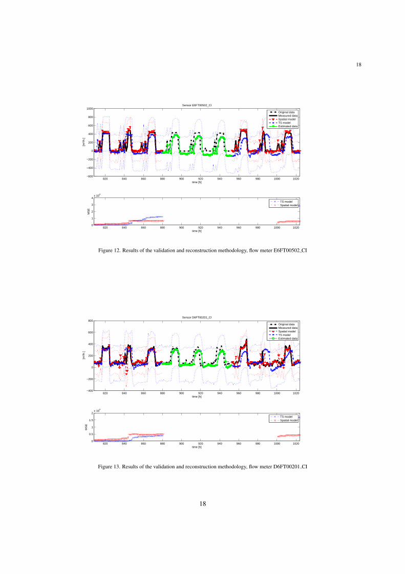
In Figure 12, a scenario involving the flow meter E6FT00502 CI is presented. In this case, a general communi-cation fault affects all the sensors, a common situation occurring in actual water monitoring systems when e.g. theconcentrator (a device collecting data from sensors installed in a particular zone) drops. Similarly as in the scenarioin Figure 11, a SM model is available using the corresponding spatially related sensors data. However, in this partic-ular case the rest of the sensors involved in the SM model (i.e. flow meter E6FT00502 CI in Figure 12, flow meterD6FT00201 CI in Figure 13) are all affected by the same communication fault, hence they are not available for datareconstruction after the communication fault occurs and, consequently, the SM model can not be considered in this

15

16

01/01 01/02 01/03 01/04 01/05

0

10

20

30

40

50

60

70

80

m³/

h.

E6FT00102_CI

01/01 01/02 01/03 01/04 01/050

200

400

600MSE

MS

E

01/01 01/02 01/03 01/04 01/05

Valid

Invalid

Validation

measuredestimatedreconstructed valuetime series

time series

test limitstest derivativetime series

Figure 10. Results of the validation and reconstruction methodology on the flow meter E6FT00102 CI

16

17

820 840 860 880 900 920 940 960 980 1000 1020−400

−200

0

200

400

600

800

time [h]

[m³/

h.]

Sensor D6FT00204_CI

Original dataMeasured dataSpatial modelTS modelEstimated data

820 840 860 880 900 920 940 960 980 1000 10200

0.5

1

1.5

2x 10

4

time [h]

MS

E

TS modelSpatial model


case due to the lack of information. Again, the only available model for reconstruction is the TSM (similarly as in thescenario in Figure 10) which is finally used for the missing data reconstruction in the scenario considered in Figure 12,based on the limited available information in this particular case.

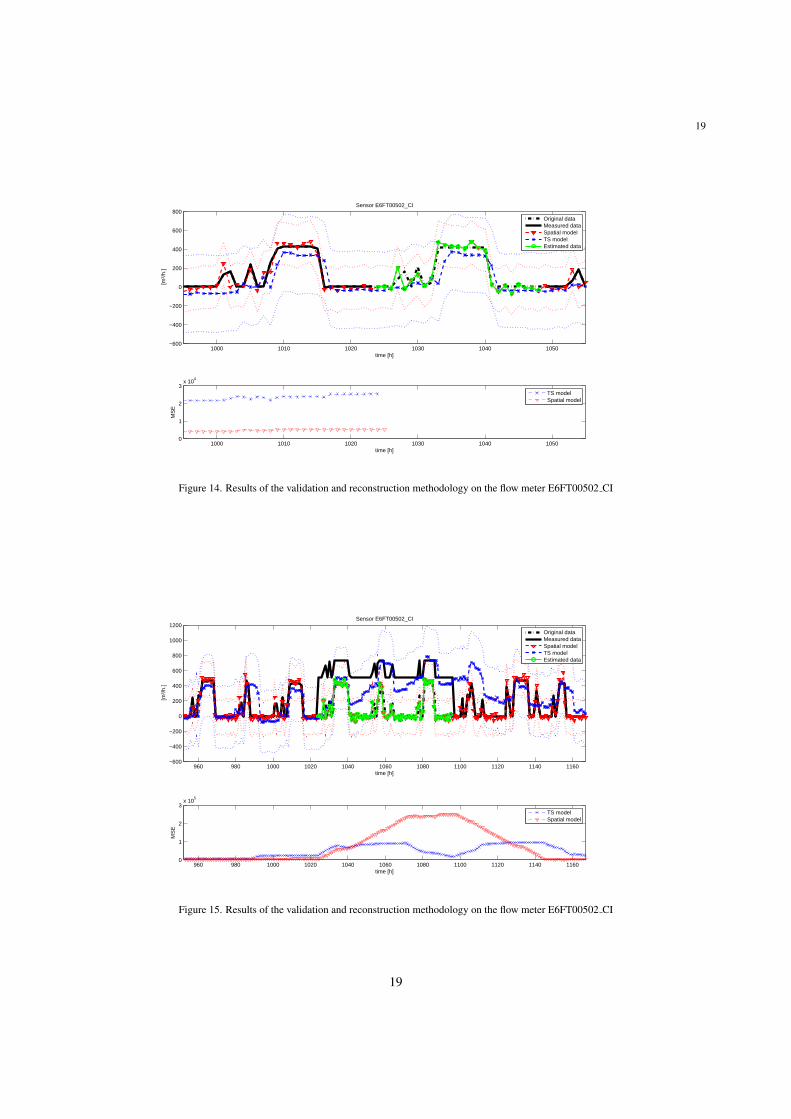
Finally, two different scenarios involving the flow meter E6FT00502 CI are considered. On the one hand, inthe scenario in Figure 14, a communication fault affecting the corresponding flow meter is presented, which doesnot transmit data in one day period (from t = 1024 h to t = 1048 h). In this particular case, the communicationfault only affects the latter sensor, hence the corresponding SM is available because the spatially related sensors (e.g.D6FT00201 CI) are not affected by this fault. In this scenario, the SM model is used for missing data reconstruction,since it performs better than the corresponding HW TSM model (bottom subplot in Figure 14). It may be notedthat the use of the SM assumes that the model input sensor measurement is faultless when the SM is used for datareconstruction. This may be assured since the input model integrity is checked by the methodology presented here atits corresponding stage and, if not verified, the validation test at this stage is not fulfilled.

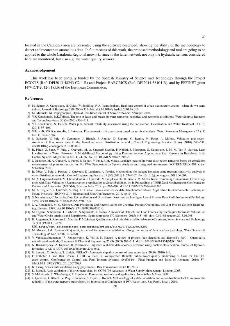
On the other hand, an offset fault of magnitude 25 % full scale affecting the flow meter E6FT00502 CI, alsocommon in this kind of sensors, is presented in Figure 15, lasting for three days (from t = 1024 h to t = 1096 h).As in the previous scenario, the SM model performs better than HW TSM before the fault is produced (see Figure 15bottom subplot) and hence it is used for invalid data estimation. In this particular scenario, it may be noted how themeasured signal is out of the SM threshold boundaries (red dotted line) for the whole fault scenario, whilst it remainsbounded by the HW TSM threshold boundaries (blue dotted line) for part of the first day after the fault is produced.This behavior is due to the adaptation of the HW TSM to the input signal, as its estimation depends on the historicrecords of the measurements, as detailed in Section 3.1. Hence, it should be considered that, when used for datavalidation, the prognosis derived from the application of the time series consistency test will expire after a certaintime after the fault is produced, when using measurement historic records.

6. Conclusions

In this paper, a data validation and reconstruction methodology is introduced to overcome the sensor problemsarising in CIS, such as water networks. The validation strategy is based on a set of data quality tests that allowto detect potentially erroneous data. Then, a reconstruction scheme is defined using SM and TSM to provide anestimation based on the model having the best fit, also providing prediction intervals for the forecasted reconstructeddata. In addition, a software tool is described to provide a homogeneous and accessible database by a user-friendlyinterface, and to apply the methodology presented here. Finally, some results obtained using data from a real network

17

18

820 840 860 880 900 920 940 960 980 1000 1020−600

−400

−200

0

200

400

600

800

1000

time [h]

[m³/

h.]

Sensor E6FT00502_CI


820 840 860 880 900 920 940 960 980 1000 10200

1

2

3

4x 10

4

time [h]

MS

E


Figure 12. Results of the validation and reconstruction methodology, flow meter E6FT00502 CI

820 840 860 880 900 920 940 960 980 1000 1020−400

−200

0

200

400

600

800

time [h]

[m³/

h.]

Sensor D6FT00201_CI


820 840 860 880 900 920 940 960 980 1000 10200

0.5

1

1.5

2x 10

4

time [h]

MS

E



18

19

1000 1010 1020 1030 1040 1050−600

−400

−200

0

200

400

600

800

time [h]

[m³/

h.]

Sensor E6FT00502_CI


1000 1010 1020 1030 1040 10500

1

2

3x 10

4

time [h]

MS

E



960 980 1000 1020 1040 1060 1080 1100 1120 1140 1160−600

−400

−200

0

200

400

600

800

1000

1200

time [h]

[m³/

h.]

Sensor E6FT00502_CI


960 980 1000 1020 1040 1060 1080 1100 1120 1140 11600

1

2

3x 10

5

time [h]

MS

E



19

20

located in the Catalonia area are presented using the software described, showing the ability of the methodology todetect and reconstruct anomalous data. In future steps of this work, the proposed methodology and tool are going to beapplied to the whole Catalonia Regional network, since in the latter network not only the hydraulic sensors consideredhere are monitored, but also e.g. the water quality sensors.

Acknowledgement

This work has been partially funded by the Spanish Ministry of Science and Technology through the ProjectECOCIS (Ref. DPI2013-48243-C2-1-R) and Project HARCRICS (Ref. DPI2014-58104-R), and by EFFINET grantFP7-ICT-2012-318556 of the European Commission.

References

[1] M. Schtze, A. Campisano, H. Colas, W. Schilling, P. A. Vanrolleghem, Real time control of urban wastewater systems - where do we standtoday?, Journal of Hydrology 299 (2004) 335–348. doi:10.1016/j.jhydrol.2004.08.010.

[2] M. Marinaki, M.; Papageorgiou, Optimal Real-time Control of Sewer Networks, Springer, 2005.[3] V.K.Kanakoudis, D.K.Tolikas, The role of leaks and breaks in water networks: technical and economical solutions, Water Supply: Research

and Technology-Aqua 50 (5) (2001) 301–311.[4] V.K.Kanakoudis, S. Tsitsifli, Water pipe network reliability assessment using the dac method, Desalination and Water Treatment 33 (1-3)

(2011) 97–106.[5] S.Tsitsifli, V.K.Kanakoudis, I. Bakouros, Pipe networks risk assessment based on survival analysis, Water Resources Management 25 (14)

(2011) 3729–3746.[6] J. Quevedo, V. Puig, G. Cembrano, J. Blanch, J. Aguilar, D. Saporta, G. Benito, M. Hedo, A. Molina, Validation and recon-

struction of flow meter data in the Barcelona water distribution network, Control Engineering Practice 18 (6) (2010) 640–651.doi:10.1016/j.conengprac.2010.03.003.

[7] R. Perez, G. Sanz, V. Puig, J. Quevedo, M. A. Cuguero-Escofet, F. Nejjari, J. Meseguer, G. Cembrano, J. M. M. Tur, R. Sarrate, LeakLocalization in Water Networks. A Model-Based Methodology Using Pressure Sensors Applied to a Real Network in Barcelona, IEEEControl Systems Magazine 34 (2014) 24–36. doi:10.1109/MCS.2014.2320336.

[8] J. Quevedo, M. A. Cuguero, R. Perez, F. Nejjari, V. Puig, J. M. Mirats, Leakage location in water distribution networks based on correlationmeasurement of pressure sensors, in: 8th IWA Symposium on System Analysis and Integrated Assessment (WATERMATEX 2011), SanSebastian, 2011.

[9] R. Perez, V. Puig, J. Pascual, J. Quevedo, E. Landeros, A. Peralta, Methodology for leakage isolation using pressure sensitivity analysis inwater distribution networks, Control Engineering Practice 19 (10) (2011) 1157–1167. doi:10.1016/j.conengprac.2011.06.004.

[10] M. A. Cuguero-Escofet, M. Christodoulou, J. Quevedo, V. Puig-Cayuela, D. Garcıa, M. Michaelides, Combining Contaminant Event Diag-nosis with Data Validation / Reconstruction : Application to Smart Buildings, in: In Proceedings of IEEE 22nd Mediterranean Conference onControl and Automation (MED14), Palermo, Italy, 2014, pp. 293–298. doi:10.1109/MED.2014.6961386.

[11] M. A. Cuguero, J. Quevedo, V. Puig, D. Garcıa, Inconsistent sensor data detection/correction: Application to environmental systems, in:Neural Networks (IJCNN), 2014 International Joint Conference on, 2014, pp. 84–90.

[12] S. Narasimhan, C. Jordache, Data Reconciliation and Gross Error Detection: an Intelligent Use of Process Data, Gulf Professional Publishing,1999. doi:10.1016/B978-088415255-2/50018-5.

[13] J. A. Romagnoli, M. C. Sanchez, Data Processing and Reconciliation for Chemical Process Operations, Vol. 2 of Process Systems Engineer-ing, Elsevier, 1999. doi:10.1016/S1874-5970(00)80015-6.

[14] M. Fagiani, S. Squartini, L. Gabrielli, S. Spinsante, F. Piazza, A Review of Datasets and Load Forecasting Techniques for Smart Natural Gasand Water Grids: Analysis and Experiments, Neurocomputing 170 (October) (2015) 448–465. doi:10.1016/j.neucom.2015.04.098.

[15] H. Jorgensen, S. Rosenrn, H. Madsen, P. Mikkelsen, Quality control of rain data used for urban runoff systems, Water Science and Technology37 (11) (1998) 113–120.URL http://www.sciencedirect.com/science/article/pii/S0273122398003230

[16] M. Mourad, J.-L. Bertrand-Krajewski, A method for automatic validation of long time series of data in urban hydrology, Water Science &Technology 45 (4-5) (2002) 263–270.

[17] V. Venkatasubramanian, R. Rengaswamy, K. Yin, S. N. Kavuri, A review of process fault detection and diagnosis: Part i: Quantitativemodel-based methods, Computers & Chemical Engineering 27 (3) (2003) 293–311. doi:10.1016/S0098-1354(02)00160-6.

[18] N. Branisavljevic, Z. Kapelan, D. Prodanovic, Improved real-time data anomaly detection using context classification, Journal of Hydroin-formatics 13 (2011) 307. doi:10.2166/hydro.2011.042.

[19] G. Lempio, C. Podlasly, T. Einfalt, NIKLAS - Automatical quality control of time series data (2000) (2010) 1–6.[20] F. Edthofer, J. Van Den Broeke, J. Ettl, W. Lettl, a. Weingartner, Reliable online water quality monitoring as basis for fault tol-

erant control, Conference on Control and Fault-Tolerant Systems, SysTol’10 - Final Program and Book of Abstracts (2010) 57–62doi:10.1109/SYSTOL.2010.5675985.

[21] K. Tsang, Sensor data validation using gray models, ISA Transactions 42 (2003) 9–17.[22] D. Burnell, Auto-validation of district meter data, in: CCWI ’03 Advances in Water Supply Management, London, 2003.[23] S. Makridakis, S. Wheelwright, R. Hyndman, Forecasting methods and applications, John Wiley & Sons, 1998.[24] J. Quevedo, J. Blanch, V. Puig, J. Saludes, S. Espin, J. Roquet, Methodology of a data validation and reconstructions tool to improve the

reliability of the water network supervision, in: International Conference of IWA Water Loss, Sao Paolo, Brazil, 2010.20

21

[25] P. R. Winters, Forecasting sales by exponentially weighted moving averages, Management Science 6 (52) (1960) 324–342.[26] R. G. Brown, Statistical Forecasting for Inventory Control, New York: McGraw-Hil, 1959.[27] J. Taylor, Short-term electricity demand forecasting using double seasonal exponential smoothing, The Journal of the Operational Research

Society 54 (8) (2003) 799–805.[28] J. W. Taylor, Triple seasonal methods for short-term electricity demand forecasting, European Journal of Operational Research 204 (1) (2010)

139–152. doi:10.1016/j.ejor.2009.10.003.URL http://linkinghub.elsevier.com/retrieve/pii/S037722170900705X

[29] C. Pegels, Exponential forecasting: Some new variations, Management Science 15 (1969) 311–315.[30] E. S. Gardner Jr., Exponential Smoothing: The State of the Art - Part II, International Journal of Forecasting 22 (4) (2006) 637–666.

URL http://www.sciencedirect.com/science/article/pii/S0169207006000392

[31] S. Gelper, R. Fried, C. Croux, Robust Forecasting with Exponential and Holt-Winters Smoothing, Journal of forecasting 29 (June 2009)(2010) 285–300. doi:10.1002/for.URL http://onlinelibrary.wiley.com/doi/10.1002/for.1125/abstract

[32] M. Basseville, I. Nikiforov, Detection of Abrupt Changes: Theory and Application, Prentice-Hall, Inc., 1993.[33] V. Puig, Fault diagnosis and fault tolerant control using set-membership approaches: Application to real case studies, International Journal of

Applied Mathematics and Computer Science 20 (4) (2010) 619–635.[34] S. X. Ding, Model-based Fault Diagnosis Techniques, Springer, 2008.

21

Documents

A Methodology and a Software Tool for Sensor Data