Embed Size (px)
DESCRIPTION
A Method of Optimal Traction Control for Farm... Osinenko 2015
Citation preview

ww.sciencedirect.com
b i o s y s t em s e n g i n e e r i n g 1 2 9 ( 2 0 1 5 ) 2 0e3 3
Available online at w
ScienceDirect
journal homepage: www.elsevier .com/locate/ issn/15375110
Research Paper
A method of optimal traction control for farmtractors with feedback of drive torque
Pavel V. Osinenko*,1, Mike Geissler 2, Thomas Herlitzius 3
Chair of Agricultural Systems and Technology (AST), Institute of Processing Machines and Mobile Machinery,
P.O. Box: 01069, Technische Universit€at Dresden (TU Dresden), Dresden, Germany
a r t i c l e i n f o
Article history:
Received 20 January 2014
Received in revised form
3 September 2014
Accepted 17 September 2014
Published online
Keywords:
Slip control
Optimal control
Infinitely variable transmissions
Traction efficiency
Traction parameters
* Corresponding author.E-mail addresses: [email protected], osi
[email protected] (T. Herlitzi1 Graduate student.2 Scientific staff member.3 Chairman.
http://dx.doi.org/10.1016/j.biosystemseng.2011537-5110/© 2014 IAgrE. Published by Elsevie
Traction efficiency of farm tractors barely reaches 50% in field operations (Renius et al.,
1985). On the other hand, modern trends in agriculture show growth of the global tractor
markets and at the same time increased demands for greenhouse gas emission reduction
as well as energy efficiency due to increasing fuel costs. Engine power of farm tractors is
growing at 1.8 kW per year reaching today about 500 kW for the highest traction class
machines. The problem of effective use of energy has become crucial. Existing slip control
approaches for farm tractors do not fulfil this requirement due to fixed reference set-point.
This paper suggests an optimal control scheme which extends a conventional slip
controller with set-point optimisation based on assessment of soil conditions, namely,
wheel-ground parameter estimation. The optimisation considers the traction efficiency
and net traction ratio and adaptively adjusts the set-point under changing soil conditions.
The proposed methodology can be mainly implemented in farm tractors equipped with
hydraulic or electrical infinitely variable transmissions (IVT) with use of the drive torque
feedback.
© 2014 IAgrE. Published by Elsevier Ltd. All rights reserved.
1. Introduction
1.1. Brief description of traction dynamics
In this section, the main factors contributing to traction effi-
ciency are discussed. First, the wheel dynamics are briefly
described. The corresponding force diagram is given in Fig. 1.
The soil reaction force Fz acts against the axle load Fz,axle and
4.09.009r Ltd. All rights reserved
thewheelweight. The horizontal soil reaction Fh (or horizontal
force) is exerted by the driving torqueMd. An opposite force on
the wheel, namely, reaction of the vehicle body, is denoted by
Fx,axle. The point of application of the soil reaction is shifted by
Dlz in direction of motion due to tyre deformation which
characterises the internal rolling resistance. Another part of
the rolling resistance Frr,e is external, due to soil deformation,
and should not be confused with the internal resistance
(Schreiber & Kutzbach, 2007).
n.de (P.V. Osinenko), [email protected] (M. Geissler),
.

Nomenclature
ht Traction efficiency
k Net traction ratio
m Horizontal force coefficient
uw Wheel revolution speed, rad s�1
r Rolling resistance coefficient
az Wheel vertical acceleration, m s�2
bt Tyre section width, m
Fh Horizontal force, N
Fz Normal force, N
Jw Wheel moment of inertia around lateral axis,
kg m2
m Vehicle mass, kg
Md Drive torque, Nm
mw Wheel mass, kg
rd Tyre dynamic rolling radius, m
s Slip
v Vehicle travelling velocity, m s�1
vw Wheel travelling velocity, m s�1
b i o s y s t em s e ng i n e e r i n g 1 2 9 ( 2 0 1 5 ) 2 0e3 3 21
The equations of motion are written as follows:
mw _vw ¼ Fh � Frr;e � Fx;axle;
Jw _uw ¼ Md � rdFh � DlzFz;
mwaz ¼ Fz �mwg� Fz;axle: (1)
The termDlzFz is substituted by rdFrr,iwhere Frr,i denotes the
internal rolling resistance (due to tyre deformation). Longitu-
dinal dynamics are characterised by several parameters: the
horizontal force coefficient m, the internal and external rolling
resistance coefficients ri,re respectively and the net traction
ratio k. They are computed with the following formulas:
Fig. 1 e Forces and torques acting on a wheel in
longitudinal motion. v!w is the wheel travelling velocity,
uw is the wheel revolution speed, mw is the wheel mass, Jwis the wheel moment of inertia around the lateral axis, rd is
the dynamic rolling radius which is the distance between
the wheel's centre and bottom points, az is the wheel
vertical acceleration.
m ¼ Fh
Fz; (2)
ri ¼Frr;i
Fz; re ¼
Frr;e
Fz(3)
k ¼ m� re; (4)
The rolling resistance coefficient is computed as sum of reand ri in (3): r ¼ re þ ri. The wheel slip is defined as follows:
s ¼ 1� jvjrdjuwj; if
��v�� � rd��uw
��;s ¼ �1þ rdjuwj
jvj ; if��v��> rd
��uw
��: (5)
It ranges from�1 (lockedwheel) to 1 (spinning on the spot).
The traction efficiency is defined as follows:
ht ¼k
kþ rð1� sÞ: (6)
Usually, the traction parameters k,r and the traction effi-
ciency ht are considered as functions of slip. Some charac-
teristic curves for different soil types are illustrated in Fig. 2.
The curves of the net traction ratio are shown without bias at
zero for simplicity. Details of zero-slip conditions have been
described by Schreiber and Kutzbach (2007).
It can be seen that, in general, maxima of ht(s) as well as
maximum achievable traction effort, characterised by k, are
different for different soil types.
1.2. Improvement of traction
The main factors, which affect the traction efficiency of farm
tractors, include the tyre pressure, properties of tyres or
tracks, the vertical load and the drive train slip. In most cases,
only the drive train slip is adjusted during the field operation,
i.e. online. The main possibilities of balancing traction effi-
ciency and productivity include drive train slip control, dy-
namic vertical load adjustment, automatic tyre pressure
Fig. 2 e Modelled traction characteristics for different soil
types (Wunsche, 2005). Solid lines e stubble, dashed lines
e wet loam, dotted lines e muddy soil. r is the rolling
resistance coefficient, ht is the traction efficiency and k is
the net traction ratio.
b i o s y s t em s e n g i n e e r i n g 1 2 9 ( 2 0 1 5 ) 2 0e3 322
control, ballasting and traction prediction. Dynamic axle load
adjustment as well as automatic tyre pressure control remain
technically difficult and are not considered in the framework
of the present paper. Traction prediction is a technique which
is used for optimising the machine configuration including
ballasting and wheel parameters based on empirical models
relating tyres and soil properties. Considerable research on
tyre empirical models and traction prediction has been con-
ducted at the US Army Engineer Waterways Experiment Sta-
tion. In characterising the tyre flexibility, a dimensionless
number, which is equal to the ratio of the tyre deflection to the
section height, was introduced. This ratio and its square, a
parameter establishing the relation of wheel load, tyre section
width and diameter, and the cone-index (CI to characterise
the soil strength) were introduced by Freitag (1965).
Wismer and Luth (1973) suggested equations with which
the tyre section width and diameter and wheel load can be
chosen from a set of parameters for high traction efficiency.
Among these parameters, CI plays the most important role. It
is obtained with a cone penetrometer in a field test. The
relation between CI, tyre parameters and wheel load is sum-
marised in a so-called wheel numeric. Based on this param-
eter, the horizontal force coefficient as a function of slip can
be predicted.
Brixius (1987) developed a more advanced approach to
traction prediction for bias-ply pneumatic tyres using curve
fitting to field test measurements. This approach is based on a
combination of the wheel numeric with tyre geometric pa-
rameters e deflection to section height ratio and width to
diameter ratio. The resulting dimensionless numeric was
called a tyre mobility number. The horizontal force coefficient
is estimated as a function of slip and mobility number.
The advantages of traction prediction have also been uti-
lised by some researchers in the form of computer programs.
Al-Hamed and Al-Janobi (2001) developed a tractor perfor-
mance program in Visual Cþþwithwhich the user can choose
a suitable configuration of a tractor by prediction of perfor-
mance parameters given the machine and tyre dimensions,
static wheel loads, transmission energy efficiency and some
other parameters as well as CI.
There have also been several modifications of the wheel
numeric and mobility numbers (see, for example, Maclaurin,
1990; Rowland & Peel, 1975). One of the recent advances in
the development of tyre mobility models was made by Hegazy
and Sandu (2013). A newmobility number was proposed based
on analysis of existing formulas as well as on experimental
data. This parameter is defined via the wheel numeric and the
square root of the difference between tyre section height and
tyre deflection divided by tyre diameter. Multiple tests have
shown great improvement of prediction of the net traction
ratio characteristic curve compared to existing approaches
including Freitag (1965); Rowland and Peel (1975); Brixius (1987).
Schreiber and Kutzbach (2008) suggested an empirical
model of the net traction ratio and rolling resistance coeffi-
cient as functions of slip with parameters computed from a
set of six factors taken as inputs e one for the tyre and five for
the soil. These factors can be easily obtained bymeasurement
or estimation for basic soil types. The advantage of this model
is that the parameters in mathematical equations for the net
traction ratio and rolling resistance coefficient, which are
abstract, are related to certain factors which have physical
meaning. The corresponding relationships were established
by analysing the characteristic curves obtained in
experiments.
As wasmentioned above, inmost cases only the drive train
slip is the subject of control and this can be performed online.
Renius (1985) made a recommendation for slip to be observed
and kept at about 10% for 4 wheel drive and 15% for twowheel
drive vehicles. Slip control can be implemented as an addi-
tional function of the three point hitch control or by means of
a traction control system (TCS) (for some recent technical
solutions and methods, refer to Boe, Bergene, & Livdahl, 2001;
Hrazdera, 2003; Ishikawa, Nishi, Okabe, & Yagi, 2012; Pranav,
Tewari, Pandey, & Jha, 2012).
The problem of optimal slip control has recently been a
field of interest for some research. Pichlmaier (2012) addresses
methods of determining drive torque in a Fendt power-split
transmission and suggests calculating the actual net traction
ratio and rolling resistance coefficient from these data
together with draft force and wheel load measurements. This
information is used to make recommendations on optimal
ballasting of the tractor.
Due to changes in soil conditions, all the approaches with a
fixed set-point are suboptimal andmight lead to unreasonably
high fuel consumption or, otherwise, low productivity. The
major objective of this paper is, therefore, to develop an al-
gorithm to find optimal slip set-points under changing soil
conditions during field operation. Such an approach should
overcome some disadvantages of the traction prediction
methods related to the lack of adaptation to the environment.
It may be used in combination with the existing slip control
algorithms.
The paper is organised as follows: Section 2 discusses
methods and techniques of obtaining the information on the
current soil conditions via the traction parameters k and r.
Section 3.1 describes the newly suggested strategy of optimal
traction control. Sections 3.2 and 3.3 introduce details of the
suggested algorithms including the net traction ration char-
acteristic curve estimation and the optimisation procedure.
The simulation results and general discussion on algorithm
tuning are presented in Section 3.4. Possible future improve-
ments of the suggested methodology are mentioned. Section
3.5 discusses the possibilities of experimental verification.
2. Materials and methods
For a traction control algorithm, which is able to adapt to
changing soil conditions, the estimation of the traction pa-
rameters k,r play a crucial role. The most important infor-
mation used in this estimation process is the drive torque
feedback which can be obtained for hydraulic or electrical
drive trains without installation of expensive torque sensors.
Low-cost solutions for torquemeasurement and calculation in
conventional mechanical drives are being developed. For
example, Li, Hebbale, Lee, Samie, and Kao (2011) suggest usage
of existing speed sensors for estimation of torque variations
on the transmission output shaft in the set-up called “virtual
torque sensor” (VTS). Wellenkotter and Li (2013) used a set of
speed sensors for estimation of the wheel torque from the

b i o s y s t em s e ng i n e e r i n g 1 2 9 ( 2 0 1 5 ) 2 0e3 3 23
relative position of the driven and undriven wheels. These
approaches give only relative values of the torque, while for
traction parameter estimation, absolute values are necessary.
For this purpose, an improvedVTSwas suggested by Li, Samie,
Hebbale, Lee, and Kao (2012). However, it requires not only
software modifications, but also an additional speed sensor
and a gear on the transmission propeller shaft before the
differential. In hydraulic drive trains, torque estimation can be
provided by oil pressure sensors. For some details and corre-
sponding aspects of traction parameter estimation, refer to
Pichlmaier (2012). The methods of drive torque estimation in
mechanical or hydraulic drive trains usually refer to calcula-
tion/measurement of the torque at the transmission output
shaft. This is appropriate if the tractor operates with a passive
implement or if the power take-off is independent of the
wheel drive. Electrified wheel drive (Barucki, 2001) is a prom-
ising candidate to substitute conventional mechanical drives
with more controllable ones. One of its configurations, elec-
trical single wheel drive (Wunsche, 2005), was implemented in
RigiTrac EWD 120 with 80 kW drive train power developed by
the AST of TU Dresden together with EAAT GmbH Chemnitz
(Geißler, Aumer, Lindner, & Herlitzius, 2010). It provides op-
tions to optimise construction of the vehicle by installing
drives directly into wheel rims. Electrical drives are also used
in construction machinery, in particular in some bulldozers
where optimal slip control problems are somewhat similar to
those of farm tractors. Drive torque feedback is obtained from
the motor electrical current and position (refer, for example,
to Meyer, Grote, & Bocker, 2007 for details).
For a four-wheel tractor, the equations of the vehicle dy-
namics in longitudinalmotion in terms of traction parameters
can be written as follows:
_uw;j ¼ 1Jw;j
�Md;j � rd;jFz;j
�mj þ ri;j
��; j ¼ 1…4 _v ¼ 1
m
Xnk¼1
mkFz;k �Xnk¼1
re;kFz;k � Fd
!; (7)
where indices j ¼ 1,2,3,4 correspond to the real left, rear right,
front left, front right wheel, Jw,1 ¼ Jw,2 and Jw,3 ¼ Jw,4 denote the
rear and front wheel inertia moments around the lateral axis
respectively, m is the tractor mass, Fd is the hitch draft force.
The values of Jw,j for j ¼ 1…4 and m are supposed to be known
and the drive torques u ¼ (Md,1,…Md,4)T are obtained via the
drive torque feedback and can be considered as exogenous
input. The wheel revolution speed and the vehicle travelling
velocity are measured which means that the output vector
and the state vector are equal: x ¼ y ¼ (uw,1,…uw,4,v)T. In
general, every single wheel has its own soil conditions and,
therefore, its own re. However, for the purposes of this paper,
it suffices to identify average re for the whole vehicle. Using
this assumption, the equation of longitudinal dynamics of the
tractor can be written as follows:
m _v ¼Xnk¼1
mkFz;k � Fd � remg: (8)
The unknown traction parameter vector is, therefore, (m1,…
m4,re)T ¼ t. Besides this, there are twelve extra unknown
variables: the dynamic rolling radii rd,1,…rd,4, the wheel loads
Fz,1,…Fz,4 and the internal rolling resistance coefficients ri,1,…
ri,4. These are arranged into an auxiliary vector
ðrd;1;…rd;4; Fz;1;…Fz;4; ri;1;…ri;4ÞT ¼ w. The parameter vector is
defined as Q ¼ ðt;wÞT. The estimation problem can be
considered in terms of an extended state vector
c ¼ ðx;QÞT2ℝ5þ5þ12:
_x ¼ fðx;u;QÞ;_Q ¼ 017�1;y ¼ x;
(9)
where fðx;u;QÞ consists of the right-hand side of the first four
equations of (7) and equation (8), 0l�1 denotes an l-length zero
vector. It is straightforward to see that (9) is not observable, i.e.
it is impossible to reconstruct x,t and w. Indeed, in order to be
observable, (9) must have an observability matrix of rank 22
(Del Vecchio & Murray, 2003). Since the original system (7) is
observable in terms of x, it is easily seen that an extended
system of type (9) is observable if the number of parametersQ
equals the number of states x which is 5. This amounts to, for
example, finding a means of eliminating w from the list of
unknowns by computing/measuring them outside of estima-
tion problem (9). There are methods of estimating the rolling
radii rd,1,…rd,4 and internal rolling resistance coefficients ri,1,…
ri,4, while the front wheel load is typically measured in the
suspension. The rear wheel load can be, thus, calculated using
the vehicle parameters. The details are discussed further in
this section. To summarise, the measurement signals
required in the estimation process are vertical load on vehicle
corners with suspension, draft force, wheel revolution speed
and vehicle traveling velocity.
All these are obtainable with conventional and/or easily
installed inexpensive sensors. The draft forcemeasurement is
typically used in the three point hitch control and is per-
formed by, for example, magnetoelastic sensors or strain
gauges installed in load pins. Usually, farm tractors have front
suspension and some have rear suspension as well which
allows wheel load to bemeasured using pressure sensors and,
possibly, induction sensors to measure the stroke displace-
ment. Gyroscopes, yaw rate sensors, accelerometers or other
relatively cheap measurement devices may be additionally
used to improve estimation. If measurement of the rear wheel
load is not available, it can be computed using the force dia-
gram in Fig. 3.
Using D'Alembert's principle for the sum of torques around
D0 in Fig. 3 yields:
Fz;r ¼ 1ld
��Fg þmaz
��lþ lr
�� Fz;f
�ld þ l
�� Fd;xhd þmaxhCG
þ�Jyy þm
�ðld þ lrÞ2 þ h2
CG
��€4y
�:
(10)
The moment of inertia around D0 is computed using the
parallel axis theorem. The dynamical components €4y; ax; az

Fig. 4 eAn example of application of the empirical formula.
Tyre radial deformation of Michelin AGRIBIB 18.4 R30. Solid
lines show measurements, dashed lines show
approximations.
Fig. 3 e Force diagram of a tractor where Jyy is the moment
of inertia around the lateral axis, Fx ¼ Fh ¡ Frr,e is the
driving force, 4y is the pitch angle.
b i o s y s t em s e n g i n e e r i n g 1 2 9 ( 2 0 1 5 ) 2 0e3 324
can be taken into account if corresponding sensors are avail-
able, e.g. gyroscope and/or accelerometer. Otherwise, they
may be ignored. For some technical solutions of piston posi-
tion measurement, refer to Albright, Bares, Shelbourn, and
Mason (2005) and Brown and Richter (2003). On the other
hand, there are many approaches to estimate wheel vertical
loads more exactly d using model identification Doumiati,
Victorino, Charara, and Lechner (2008) developed an identifi-
cation approach for vehicle vertical dynamics using only
standard sensors: accelerometers and relative suspension
sensors. Here, lateral load transfer is considered and all four
wheel loads are estimated. The approach is based on Kalman
filter. Moshchuk, Nardi, Ryu, and O'dea (2008) used suspension
displacement sensors, which are cheap and easy-to-install, to
estimate wheel load together with vehicle vertical accelera-
tion using simple formulas and a differentiator filter. Ray
(1995) suggested an extended Kalman filter for the same pur-
poses. As in the previous case, suspension displacement
sensors are used.
The tyre dynamic rolling radius is defined as follows:
rd ¼ r0 � Df �; (11)
where r0 is the tyre unloaded radius and Df* is the tyre
deflection on a loose soil which can be estimated using some
geometric tyre-ground contact model (for example, cylindri-
cal). It is usual to approximate Df* from that on a rigid surface.
The latter is an open subject of investigations which include
both empirical models and sensor design. Generally, Df de-
pends nonlinearly on the vertical load and the nonlinearity is
due to the tyre material and construction. Schmid (1995)
developed iterative numerical algorithms to derive the tyre
deflection Df* on a loose soil and contact surface length from
Df and tyre spring constant using a cylindrical model. In this
paper, the tyre dynamic rolling radius (11) is approximated
using Df instead of Df*. Guskov et al. (1988, p. 40) uses a linear
empirical formula for the tyre deflection on a rigid surface Df
as follows:
Df ¼ Fz
2p$105$pt
ffiffiffiffiffiffiffiffiffiffiffiffiffiffibt=2r0
p ; (12)
where pt is the tyre inflation pressure in bar and bt is the tyre
sectionwidth. Example of application of this formula is shown
in Fig. 4.
It is seen that at vertical loads recommended for certain
inflation pressures, the empirical formula provides estimates
which may be appropriate in some applications. However, for
some tyres, the accuracymight be poor and vertical deflection
measurement followed by regression analysis might be
necessary. For some further estimation approaches, refer to
Rashidi, Azadeh, Jaberinasab, Akhtarkavian, and Nazari
(2013), Rashidi, Sheikhi, & Abdolalizadeh (2013), Lyasko
(1994). Lyasko (1994) also provides methods of estimating the
tyre contact area width and length. The internal rolling
resistance coefficient ri does not change significantly and
mainly depends on the tyre inflation pressure. On a loose soil,
it can be estimated from that on a rigid surface (see, for
example, Schreiber & Kutzbach, 2007; Schreiber & Kutzbach,
2008). In this paper, ri is assumed as a known parameter. For
it, the estimation of traction parameters t the wheel and
wheel inertia indices can be omitted. The wheel rotational
dynamical component Jw _uw can be estimated from the wheel
speed measurement using a differentiator filter. Otherwise,
model identification approaches can be used (for some of
them, refer to Ono et al., 2003; Dakhlallah, Glaser, Mammar, &
Sebsadji, 2008; Osinenko, 2013; Canudas-de Wit, Petersen, &
Shiriaev, 2003). Finally, m is computed by:
m ¼ Md � Jw _uw
rdFz� ri: (13)
Supposing that the horizontal force coefficients mk are
estimated, re can be computed similarly to (13) as follows:
re ¼1mg
Xnk¼1
mkFz;k � Fd
!� _vg: (14)
The net traction ratio k in terms of the whole vehicle can be
computed by:
k ¼ 1mg
Xnk¼1
mkFz;k � re: (15)

b i o s y s t em s e ng i n e e r i n g 1 2 9 ( 2 0 1 5 ) 2 0e3 3 25
3. Results and discussion
3.1. Optimal traction control strategy
The suggested methodology of this paper extends a slip con-
trol algorithm, realised either by the three point hitch, TCS or
some other method, by incorporating an optimality condition
depending on two factors: the traction efficiency and perfor-
mance. The modification is made in the form of a supervisor
which estimates the traction parameters online using the
drive torque feedback andmeasurement signals from sensors
which are often available. The estimated values are utilised in
estimation of the net traction ratio characteristic curve. The
optimality functional is formulated in terms of this curve, the
corresponding traction efficiency curve and one parameter to
balance these two factors. Uniqueness of a maximum of the
functional is shown. The computed optimal drive train slip
set-point is transmitted to the slip control method. The latter
together with the supervisor constitute the suggested optimal
traction control. This strategy is not used to predict the
optimal operating conditions or to define the machine and/or
tyre dimensioning as it is performed in traction prediction.
The goal of the approach is to change the set-point adaptively
during the field operation. To summarise, the suggested
optimal traction control includes the following steps:
1. obtain machine parameters (wheel radius, dimensioning
etc.) and operation strategy (efficiency or productivity),
2. perform measurements,
3. estimate the traction parameters,
4. estimate the net traction ratio characteristic curve,
5. compute the optimum of slip,
6. perform slip control with the computed optimal set-point
7. check soil condition change.
The optimisation in step 5 is one-dimensional and has
polynomial time complexity which indicates that the algo-
rithm is efficient (Cobham, 1965). Supposing the optimum is
located within the unit interval and given the tolerance of 1/n
for some natural number n (that is, the outcome of the algo-
rithm and the actual optimum will differ at most by 1/n), the
worst-case time complexity is O(n). The estimation process in
step 4 cannot be unambiguously performed with classical
model identification approaches from the current operating
point and generally requires some curve fitting algorithm
from a set of estimated points. Such a procedure may
comprise multidimensional optimisation which might be
computationally expensive. On the other hand, some parts of
the estimation can be carried out offline and the obtained
parameters can be used further online without considerable
hardware requirements. A variant of a such method is
currently used in the suggested optimal traction control and
comprises a set of 15 parameters obtained offline from typical
net traction ratio characteristic curves. The proposed algo-
rithm is able to estimate the curve given one slip-k tuple. The
set of 15 parameters is built-in and not used as an input. This
is different from several traction prediction algorithms where
the user defines some empiric or measured wheel and soil
parameters with which the characteristic curve can be
obtained. Instead, the user only defines the strategy via one
parameter ranging from zero to one which corresponds to
emphasising traction efficiency or performance. The only
purpose of the parameter set used in step 4 is to reduce
computational load and tomake the algorithmappropriate for
conventional microcontrollers. The same goal may be ach-
ieved by tuning the tolerance of the method in step 7 where
the soil condition changes are detected. Increasing a
threshold, beyond which changes in soil conditions are indi-
cated, allows for more sparse optimum calculations and less
computational load. The details of the soil condition change
checking are described in Section 3.3.
3.2. Estimation of the net traction ratio characteristiccurve
The traction parameter estimation discussed in Section 2
provides information only about current operation condi-
tions, i.e. tuples of type (s,k) and (s,ht) where s denotes current
slip. On the other hand, in order to define the optimal traction
control set-point, it is reasonable to obtain information of the
characteristic curves k(s),ht(s) over a wide range of slip. This
can be done purely online by gathering a set of estimated
tuples including the zero-slip tuple ð0;�breÞ where bre denotesthe estimated external rolling resistance coefficient. The set of
tuples can be approximated using some suitable mathemat-
ical model. Such an algorithm can be roughly classified as
“expensive” when considering computational complexity
compared to a “cheap” algorithm, which is now discussed.
Several models for k as a function of slip that can be found in
the literature consist of a constant, a linear and an exponen-
tial term. For example, Schreiber and Kutzbach (2007) used the
following equation:
kðsÞ ¼ aþ ds� b expðcsÞ; (16)
where a, b, c, d are the unknown parameters. In general,
characteristic curves have a bias at zero depending on the
external rolling resistance coefficient. Therefore, Schreiber
and Kutzbach (2007) substituted b � a with re. A similar
function was used by Burckhardt and Reimpell (1993) for the
horizontal force coefficient. In this paper, the bias is consid-
ered separately by introducing the estimated re. The formula
(16) is modified by excluding the bias and introducing the
second exponential term instead of the linear term in the
following way:
k0ðsÞ ¼ a0 � c0 expð�b0sÞ � c1 expð�b1sÞ; (17)
where a0, c0, b0, c1, b1 are the unknown parameters. With such
a formula, appropriate accuracy of approximation can still be
achieved and different behaviour in the low- and in the high-
slip range can be captured. On the other hand, it can provide
the necessary convexity property for the optimisation prob-
lem to guarantee uniqueness of solution. Details will be dis-
cussed in the next section. The resulting characteristic curve
k(s) is equal to k0(s)�re.
The idea of the “cheap” algorithm is to provide parameters
q ¼ (a0,c0,b0,c1,b1)T of a k0-curve given one user-defined point
(s,k0), i.e. to find q ¼ q(s,k0). For this purpose, a set of simplified
characteristic curves which roughly classify soil conditions

b i o s y s t em s e n g i n e e r i n g 1 2 9 ( 2 0 1 5 ) 2 0e3 326
from “bad” to “good” was assumed. Such classification has
been used by several authors (see, for example, Kutzbach,
1982; Renius, 1985). In the current set-up, seven typical
curves out of a range from stubble to muddy soil given by
S€ohne (1964, p. 45) were assumed.
Such a set of curves approximately describes the behaviour
of the net traction ratio in awide range of soil conditions. First,
the model (17) is fitted to the given curves. Second, additional
curves are constructed between the original set. When the
input tuple (s,k0) is received, two neighbouring curves are
found. The estimated curve is obtained via interpolation. This
procedure is somewhat analogous to forming a lookup table of
curves and serves for computational load reduction.
The initial curves are shown in Fig. 5. The bias at zero is
removed at this stage and introduced after the approximation
process. The curves are given for the range of slip between
zero and 50%which is supposed to be enough for practical use
of traction control. At the first step, parameters q of model
eq:kappa-model were fitted to given k0-curves numerically
using LevenbergeMarquardt algorithm (Marquardt, 1963):
minimise kk0 � ða0 � c0 expð�b0sÞ � c1 expð�b1sÞÞk22;subject to a0; c0;b0; c1;b1 � 0;
(18)
where���� � ����
2denotes Euclidean norm. For a discrete set of N
points of a given k0-curve, the objective amounts to:
XNj¼1
�k0j �
�a0 � c0 exp
��b0sj�� c1 exp
��b1sj���2
: (19)
This problem is non-convex since
(a0 � c0 exp(�b0s) � c1 exp(�b1s)) is a non-convex function for
arbitrary (a0, c0, b0, c1, b1), therefore, only a local solution is
possible. Nevertheless, a global solution is not crucial at this
stage. Satisfactory accuracy can be achieved by changing
initial conditions and running the optimisation algorithm
repeatedly. For all given curves, the normalised root-mean-
square error (NRMSE) of fitting.
Fig. 5 e Initial set of k′-curves.
NRMSE¼ 1
maxj
�k0j
��minj
�k0j
�ffiffiffiffiffiffiffiffiffiffiffiffiffiffiffiffiffiffiffiffiffiffiffiffiffiffiffiffiffiffiffiffiffiffiffiffiffiffiffiffiffiffiffiffiffiffiffiffiffiffiffiffiffiffiffiffiffiffiffiffiffiffiffiffiffiffiffiffiPN
j¼1
�k0j�k0ða0;c0;b0;c1;b1;sÞ
�2N
vuut(20)
was below 0.1%. Number of data points of each k0-curve was
N ¼ 50. The solutions are denoted by bqj ¼ðba0j;bc0j; bb0j;bc1j; bb1jÞ; i.e.bq1j ¼ ba0j; bq2j ¼ bc0j; bq3j ¼ bb0j; bq4j ¼ bc1j; bq5j ¼ bb1j; j ¼ 1…7 and first
index denotes the number of the parameter, second denotes
the number of the curve. Further, each parameterwas fitted as
a function of the net traction ratio k0 at s1 ¼ 50%. These values
are indexed for each of seven curves in the following manner:
k01;…k07. It was observed that appropriate accuracy could be
achieved using quadratic polynomial model:�ai;0 þ ai;1k
0 þ ai;2k02�; i ¼ 1:::5; (21)
where ai,0, ai,1, ai,2 are the subparameters. In this case, fitting
was done using polynomial approximation by means of
Vandermonde matrix for each parameter:
Vi ¼
0BBB@1 k01
�k01�2
1 k02�k02�2
« « «
1 k07�k07�21CCCA; i ¼ 1…5: (22)
Further, the following matrix equations are solved:
Vipi ¼�bqi1…
bqi7�T; i ¼ 1…5; (23)
where pi ¼ (ai,0,ai,1,ai,2)T is the polynomial coefficient vector.
The results for parameters q depending on k0 at 50% slip for
seven curves are shown in Fig. 6.
Approximation NRMSE of parameters a0,c0,b0,c1,b1 was
0.04, 0.12, 0.94, 1.5 and 0.07% respectively. Using these ap-
proximations, n ¼ 25 curves were built (see Fig. 5). The pa-
rameters q are now approximated as functions of curve index
k:k0k(s), k ¼ 1…n. As in (21), usage of quadratic polynomial
models.
qiðkÞ ¼ bi;0 þ bi;1kþ bi;2k2; i ¼ 1…5; (24)
provided appropriate accuracy. Here, bi,0, bi,1, bi,2 are the sub-
parameters. Approximation NRMSE of parameters a0, c0, b0, c1,
Fig. 6 e Parameters q depending on k′ at s ¼ 50%. Dotted
lines show quadratic approximation. Parameter values are
indicated by circles.
b i o s y s t em s e ng i n e e r i n g 1 2 9 ( 2 0 1 5 ) 2 0e3 3 27
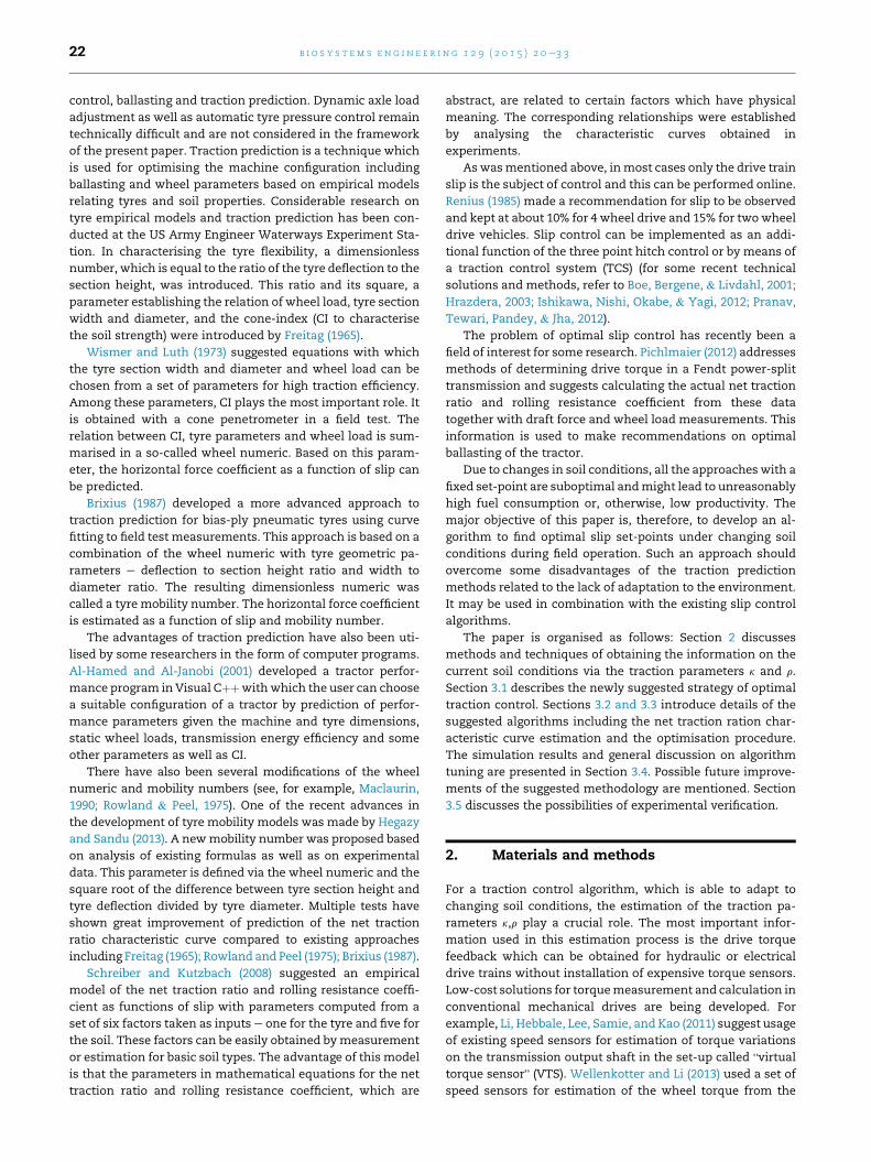
b1 were 0.07, 0.15, 1.14, 0.05 and 0.18% respectively. The last
step is to determine curve index k for the given point (s,k0).
This is performed using the algorithm in Fig. 7. If a relevant
curve index is not found, the algorithm returns flag
UPD_CON ¼ 0 and UPD_CON ¼ 1 otherwise. In the latter case,
the set-point will not be updated. Further explanation is given
in the next section. All numerical procedures were performed
in MATLAB©R2010a on a platform with AMD Athlon™Pro-
cessor/2148 Mhz and 1 Gb RAM.
Theworst-case time complexity of the algorithm in Fig. 7 is
O(n). The k0-curves estimatedwith use of thismethodology are
without bias at zerowhich, in fact, corresponds to the external
rolling resistance coefficient re (see Schreiber & Kutzbach,
2007 for detail). Therefore, an offset should be performed
before estimation, namely, the current operating point (s,k)
should be set to (s,k þ re) as input to the algorithm in Fig. 7.
3.3. Optimal traction control algorithm
The suggestedmethodology of this paper implies a slip control
algorithm with optimal set-point computation. Slip control
itself can be performed by means of the three point hitch or
drive trains. Consider the following optimisation problem:
maximise ðover sÞ htðs; q; re; riÞ;maximise ðover sÞ kðs; q; reÞ;
subject to 0 � s � s1;(25)
Fig. 7 e Flowchart of the algorithm for finding a relative
curve index and parameters k′-curve parameters.
where s1 ¼ 50% as in the previous section. The objectives are
defined as follows:
kðs; q; reÞ ¼ a0 � c0 expð�b0sÞ � c1 expð�b1sÞ � re; (26)
htðs; q; re; riÞ ¼kðs; q; reÞ
kðs; q; reÞ þ re þ rið1� sÞ: (27)
The optimisation problem can be scalarised and reformu-
lated in the following way:
maximise ðover sÞ skðs; q; reÞ þ ð1� sÞhtðs; q; re; riÞ;subject to 0 � s � s1;
(28)
where s ¼ 0…1 is a user-defined parameter which character-
ises the operation strategy ranging from maximal traction
efficiency to maximal productivity.
Theorem 1. Consider optimisation problem (28) together with (26),
(27). Let the following conditions hold:
1. a0, c0, b0, c1, b1 � 0,
2. at least one of tuplets (c0,b0) and (c1,b1) is not equal to (0,0),
3. k(s1,q,re) þ re þ ri > 0,
then the objective function of (28) has a unique maximum on ð~s; s1�for ~s defined by a0 � c0 expð�b0~sÞ � c1 expð�b1~sÞ þ ri ¼ 0:
Proof. Consider function kðsÞ ¼ a0 � c0 expð�b0sÞ � c1expð�b1sÞ � re: Its derivative
ðkðsÞÞ0 ¼ b0c0 expð�b0sÞ þ b1c1 expð�b1sÞ (29)
is strictly positive since b0c0, b1c1 � 0 and at least one of the
exponential terms is strictly positive. The second derivative is:
ðkðsÞÞ00 ¼ �b20c0 expð�b0sÞ � b2
1c1 expð�b1sÞ< 0 (30)
for any s. Therefore, (26) is strictly concave and increasing.
Consider now function:
hðsÞ ¼ kðsÞkðsÞ þ r
; (31)
where r ¼ re þ ri. Function k(s) þ r ¼ a0 � c0 exp(�b0s)
� c1 exp(�b1s) þ ri is strictly increasing and since
lims/�∞
ðkðsÞ þ rÞ ¼ �∞ and kðs1Þ þ r>0 (32)
has a unique zero ~s. The derivative of h(s) is computed as
follows:
ðhðsÞÞ0 ¼ ðkðsÞÞ0ðkðsÞ þ rÞ � k0ðsÞkðsÞðkðsÞ þ rÞ2 ¼ rðkðsÞÞ0
ðkðsÞ þ rÞ2 : (33)
It can be seen that ðhðsÞÞ0 > 0 for any ss~s since ðkðsÞÞ0 > 0.
The second derivative is:
ðhðsÞÞ00 ¼ r
ðkðsÞÞ00
ðkðsÞ þ rÞ2 � 2
�ðkðsÞÞ0�2ðkðsÞ þ rÞ3
!: (34)
The first term in parentheses ðkðsÞÞ00=ðkðsÞ þ rÞ2 is strictly
negative for any s according to (30). Term �2ðððkðsÞÞ0Þ2=ðkðsÞ þ rÞ3Þ is strictly negative for s> ~s. Therefore, h(s) is strictly
concave for s> ~s. Consider function:

b i o s y s t em s e n g i n e e r i n g 1 2 9 ( 2 0 1 5 ) 2 0e3 328
gðsÞ ¼ hðsÞð1� sÞ; (35)
Its second derivative reads as:
ðgðsÞÞ00 ¼ ðhðsÞÞ00 ð1� sÞ � 2ðhðsÞÞ0: (36)
It can be noticed that (1 � s) > 0 for s⩽s1 ¼ 0:5. Therefore,ðhðsÞÞ00 ð1� sÞ<0 and since ðhðsÞÞ0 >0 for ~s< s⩽s1; function
ht(s,q,re,ri)¼ g(s) is strictly concave for ~s< s⩽s1. For any s¼ 0…1,
the objective of (28) is either equal to k(s) or g(s) or their posi-
tive weighted sum. On interval ð~s; s1�, it has a unique
maximum. ∎
Remark 2. Conditions 1., 2. and 3. of the theorem imply that
the k-curve is not a constant and k(s,q,re) þ re þ ri has a zero~s< s1. Normally, according to Schreiber and Kutzbach (2007),
the net traction ratio is equal to the external rolling resistance
coefficient at zero slip: k(0,q,re) ¼ �re. In this case, ~s<0 and
optimisation problem (28) together with its constraint are
well-defined, i.e. 0 � s � s1 is within the domain of (27) and
there is a unique solution. However, due to inaccuracy of k-
curve approximation (see Section 3.2), equality k(0,q,re) ¼ �re
might not hold. Therefore, the lower bound of constraint
Fig. 8 e Flowchart of the optim
0 � s � s1 might need to be tightened to some s0. This can be
done with the following algorithm:
1. set s0: ¼ 0%,
2. if k(s0,q,re) > �(re þ ri), then finish, else s0: ¼ s0 þ Ds, repeat,
where Ds is a tuning parameter which can be set to 0.5% for
instance. A solution to (28) can be found by some algorithm
which would not “fall off” the constraint, e.g. by Golden Sec-
tion method (Kiefer, 1953).
If s ¼ 0, the optimisation problem amounts to finding the
maximum of ht(s)-curve. If s ¼ 1, the solution is the maximum
of k(s)-curve. Further, several strategies of optimal traction
control are possible. Optimisation can be performed contin-
uously during the operationwhichmight require considerable
computational resources. On the other hand, it is reasonable
to compute set-points for a slip control system at discrete
moments of time when changes in soil conditions are
noticeable. The suggested methodology is summarised in the
flowchart in Fig. 8 which is a modified variant from Osinenko
(2013). The algorithm starts by acquiring vehicle and tyre pa-
rameters. Some of the values, like tyre unloaded radius,
al slip control algorithm.

Fig. 9 e Traction efficiency, net traction ratio, drive train (thick solid lines), traction power (thin solid lines) and power losses
(dashed lines) as functions of slip for three soil conditions.
b i o s y s t em s e ng i n e e r i n g 1 2 9 ( 2 0 1 5 ) 2 0e3 3 29
section width etc., can be programmed into ROM of a micro-
controller since they are changed rarely, e.g. when the vehicle
is equipped with other wheels. Information about the tyre air
pressure must be provided by the operator, i.e. driver, or by
means of sensors.
In the case where a relevant characteristic curve is not
found (UPD_CON ¼ 0), the algorithm does not update the set-
point and slip control is performed with the previously
computed reference. This step is needed to process a failure in
Fig. 7 and lasts for STD_T seconds after which the algorithm
tries to find a curve again. The parameter STD_T can be
adjusted. Tuning parameter Dk is used to detect noticeable
changes in soil conditions. It can be adjusted by the user.
Lower values would mean more frequent computation of set-
points andmake the control systemmore sensitive to changes
in soil conditions and vice versa.
3.4. Simulation results
RigiTrac EWD 120 was used as an example tractor for testing
the suggested control scheme. Three soil conditions roughly
Fig. 10 e Computed optimal slip (dashed lines), traction power
functions of the user-defined strategy s.
ranging from “bad” to “good” were simulated. They are
denoted as Soil I, II and III and for each, simulation was per-
formed to obtain curves (s,k),(s,ht) as well as traction power
(s,Ptr), drive train power (s,Pdrive) and power losses
(s,Ploss) ¼ (s,Pdrive � Ptr). Results are shown in Fig. 9.
First, the characteristic k-curveswere approximated offline
using (18) to investigate the influence of the user-defined
strategy s on the traction efficiency and performance. The
results are shown in Fig. 10. The values at s ¼ 0 have a clear
meaning, they correspond to the maxima of ht. In most ap-
plications, suitable operating points, which provide a
reasonable trade-off between the traction efficiency and per-
formance, lie slightly beyond these values (Wismer & Luth,
1973). Therefore, s should be set slightly above zero. It is
seen that values of 0.2e0.3 roughly correspond to the slip at
which the growth of the power losses is moderate for all three
soils. Beyond these values, the growth of Ploss increases as ht
plays a less dominant role. Therefore, sz 0.25 should satisfy a
wide range of applications.
In the online phase, traction parameters were estimated as
described in Section 2. Dynamical processes Jw _uw andm _vwere
(solid black lines) and power losses (solid grey lines) as

Fig. 12 e Estimated external rolling resistance coefficient
and net traction ratio (dashed grey lines). True values are
shown as solid black lines.
b i o s y s t em s e n g i n e e r i n g 1 2 9 ( 2 0 1 5 ) 2 0e3 330
estimated by filtering the velocity and wheel speed measure-
ments using a 4th-order Butterworth low-pass filter with cut-
off frequency equal to 5 Hz and taking discrete derivatives
using the following discrete transfer function:
WðzÞ ¼ z� 1Tsz
;
where z denotes unit delay and Ts is the simulation step.
Change of soil conditions was simulated by step functions.
Parameter Dk was set to 0.075, the working depth and working
width were fixed at 75 mm and 5 m respectively. Slip control
was performed by means of a TCS using the algorithm from
Sunwoo (2004). The vehicle starts on soil I with a conventional
set-point of 10%. For 5 s, the supervisor is switched off for
initial collecting of information. The following phases are of
interest (see Fig. 11):
� phase 1 (0e5 s): the supervisor is switched off, the slip
controller works with 10% reference which corresponds to
the conventional control, the soil conditions correspond to
Soil I;
� phase 2 (5e16 s): supervisor computes and sets the refer-
ence for the slip control system;
� phase 3 (16e29 s): at 16 s, soil conditions change from I to II,
a new set-point is computed in about 1 s and then stays
fixed;
� phase 4 (29e40 s): at 29 s, soil conditions change from II to
III, a new set-point is computed in about 1.5 s and then
stays fixed;
Due to the vertical load transfer, the drive torques on rear
and front wheels are different in order to keep the desired slip.
Estimation of traction parameters is shown in Fig. 12. It is seen
that the transient phases in computation of new set-points in
Fig. 11 e Vehicle dynamics under changing soil conditions
and optimal traction control. Rear drive torques are shown
as black solid lines, front drive torques are shown as grey
solid lines.
Fig. 11 roughly correspond to the transient phases in esti-
mated re and k. After the soil conditions stabilse, the updating
of the set-points stops.
The results of k-curve approximation for soils I, II and III are
shown in Fig. 13. NRMSE for all three cases is below 1.3%.
Optimal traction control was performed with s ¼ 0.25. Results
for soil I are shown in Table 1.
It is seen that with optimal traction control, the traction
efficiency is almost the same as for conventional traction
control, while the net traction ratio and traction power are
23% and 43% higher respectively. The productivity is 8%
higher. The growth of the power losses is about 44%, which is
about as high as growth of the traction power. With no con-
trol, operating at full drive train power, the traction power
grew 19%, while the power losses were 33% higher. For some
practical purposes, such excessive growth of power losses
might be unreasonable since the increase of traction power is
only one half the increase in loss. Therefore, the value of slip
at about 13e14 % can be recognised as optimal for soil I.
Table 2 contains results for soil II. In this case, even the
maximum of the traction efficiency is not achieved with
conventional traction control. Optimal control showed 2.4
times the traction power than with 10% slip. The growth of
power losses is less, i.e. twice as high as with conventional
traction control. The productivity is 56% higher. Working at
10% slip is unreasonable and the tractor simply does not
achieve effective drive train power. However, further increase
of Pdrive becomes unprofitable since the traction power grows
42% higher, while the power losses are 61% higher.
Fig. 13 e Online estimation of k-curves (dashed grey lines).
Results of the simulation are shown as solid black lines.
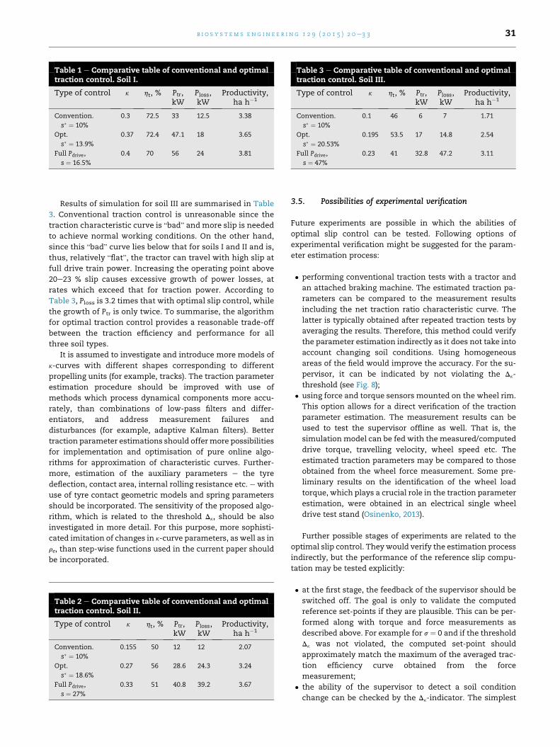
Table 1 e Comparative table of conventional and optimaltraction control. Soil I.
Type of control k ht, % Ptr,kW
Ploss,kW
Productivity,ha h�1
Convention.
s� ¼ 10%
0.3 72.5 33 12.5 3.38
Opt.
s� ¼ 13:9%
0.37 72.4 47.1 18 3.65
Full Pdrive,
s ¼ 16:5%
0.4 70 56 24 3.81
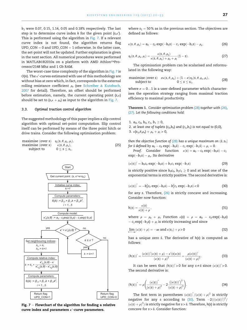
Table 3 e Comparative table of conventional and optimaltraction control. Soil III.
Type of control k ht, % Ptr,kW
Ploss,kW
Productivity,ha h�1
Convention.
s� ¼ 10%
0.1 46 6 7 1.71
Opt.
s� ¼ 20:53%
0.195 53.5 17 14.8 2.54
Full Pdrive,
s ¼ 47%
0.23 41 32.8 47.2 3.11
b i o s y s t em s e ng i n e e r i n g 1 2 9 ( 2 0 1 5 ) 2 0e3 3 31
Results of simulation for soil III are summarised in Table
3. Conventional traction control is unreasonable since the
traction characteristic curve is “bad” and more slip is needed
to achieve normal working conditions. On the other hand,
since this “bad” curve lies below that for soils I and II and is,
thus, relatively “flat”, the tractor can travel with high slip at
full drive train power. Increasing the operating point above
20e23 % slip causes excessive growth of power losses, at
rates which exceed that for traction power. According to
Table 3, Ploss is 3.2 times that with optimal slip control, while
the growth of Ptr is only twice. To summarise, the algorithm
for optimal traction control provides a reasonable trade-off
between the traction efficiency and performance for all
three soil types.
It is assumed to investigate and introduce more models of
k-curves with different shapes corresponding to different
propelling units (for example, tracks). The traction parameter
estimation procedure should be improved with use of
methods which process dynamical components more accu-
rately, than combinations of low-pass filters and differ-
entiators, and address measurement failures and
disturbances (for example, adaptive Kalman filters). Better
traction parameter estimations should offermore possibilities
for implementation and optimisation of pure online algo-
rithms for approximation of characteristic curves. Further-
more, estimation of the auxiliary parameters e the tyre
deflection, contact area, internal rolling resistance etc. e with
use of tyre contact geometric models and spring parameters
should be incorporated. The sensitivity of the proposed algo-
rithm, which is related to the threshold Dk, should be also
investigated in more detail. For this purpose, more sophisti-
cated imitation of changes in k-curve parameters, as well as in
re, than step-wise functions used in the current paper should
be incorporated.
Table 2 e Comparative table of conventional and optimaltraction control. Soil II.
Type of control k ht, % Ptr,kW
Ploss,kW
Productivity,ha h�1
Convention.
s� ¼ 10%
0.155 50 12 12 2.07
Opt.
s� ¼ 18:6%
0.27 56 28.6 24.3 3.24
Full Pdrive,
s ¼ 27%
0.33 51 40.8 39.2 3.67
3.5. Possibilities of experimental verification
Future experiments are possible in which the abilities of
optimal slip control can be tested. Following options of
experimental verification might be suggested for the param-
eter estimation process:
� performing conventional traction tests with a tractor and
an attached braking machine. The estimated traction pa-
rameters can be compared to the measurement results
including the net traction ratio characteristic curve. The
latter is typically obtained after repeated traction tests by
averaging the results. Therefore, this method could verify
the parameter estimation indirectly as it does not take into
account changing soil conditions. Using homogeneous
areas of the field would improve the accuracy. For the su-
pervisor, it can be indicated by not violating the Dk-
threshold (see Fig. 8);
� using force and torque sensors mounted on the wheel rim.
This option allows for a direct verification of the traction
parameter estimation. The measurement results can be
used to test the supervisor offline as well. That is, the
simulation model can be fed with the measured/computed
drive torque, travelling velocity, wheel speed etc. The
estimated traction parameters may be compared to those
obtained from the wheel force measurement. Some pre-
liminary results on the identification of the wheel load
torque, which plays a crucial role in the traction parameter
estimation, were obtained in an electrical single wheel
drive test stand (Osinenko, 2013).
Further possible stages of experiments are related to the
optimal slip control. They would verify the estimation process
indirectly, but the performance of the reference slip compu-
tation may be tested explicitly:
� at the first stage, the feedback of the supervisor should be
switched off. The goal is only to validate the computed
reference set-points if they are plausible. This can be per-
formed along with torque and force measurements as
described above. For example for s ¼ 0 and if the threshold
Dk was not violated, the computed set-point should
approximately match the maximum of the averaged trac-
tion efficiency curve obtained from the force
measurement;
� the ability of the supervisor to detect a soil condition
change can be checked by the Dk-indicator. The simplest

b i o s y s t em s e n g i n e e r i n g 1 2 9 ( 2 0 1 5 ) 2 0e3 332
variant of such tests would be to drive on tilled/untilled
areas of the field;
� different optimal set-points provided by the supervisor
may be checked for general types of soil, e.g. wet/dry,
sandy/clay etc. The values for the “worse” soils should be
greater, than for the “better” ones;
� if the values computed by the supervisor are plausible in all
previous experiments, the optimal slip control can be
tested fully online. In this case, such parameters as the fuel
consumption per unit area or productivity may be
compared.
It is expected that even under uncertainties of the tyre
contact parameters, internal rolling resistance etc., the pro-
posed control scheme should be able to produce reasonable
reference set-points. All suggested experiments may be
similarly carried out with a construction machine like a bull-
dozer. Another important possibility is to verify the optimal
slip control in a laboratory for testing tyres on a loose soil.
Such a laboratory would contain, for example, a specially built
gutter filled with a soil and equipment able to drive the tyre in
the gutter.
4. Conclusions
In this paper, a new strategy for optimal traction control is
suggested. The approach is based on traction parameter
estimation via drive torque feedback. It is able to estimate
whole characteristic curves of the net traction ratio against
slip using a set of model parameters. Traction control is based
on optimisation which is performed in periods of noticeable
change of soil conditions. The suggested methodology can be
used for off-road vehicles where the problems of traction ef-
ficiency are crucial. Simulation results showed better perfor-
mance of optimal traction control than existing methods.
Acknowledgement
The authors would like to thank A.Gunther, the AST, and K.
R€obenack, the Chair for Control Engineering of TU Dresden,
for their valuable suggestions and comments. Special thanks
go to H. D€oll for themajor ideas in developing the algorithm of
the net traction ratio characteristic curve approximation. The
research was conducted in the framework of the agriculture
electrification project at the AST of TU Dresden.
r e f e r e n c e s
Al-Hamed, S., & Al-Janobi, A. (2001). A program for predictingtractor performance in visual cþþ. Computers and Electronics inAgriculture, 31(2), 137e149.
Albright, L., Bares, M., Shelbourn, W., Mason, S., (2005). Methodand apparatus for stroke-position sensor for hydrauliccylinder. WO Patent 2,005,038,270.
Barucki, T. (2001). Optimierung des Kraftstoffverbrauches und derDynamik eines dieselelektrischen Fahrantriebes fur Traktoren[Optimization of fuel consumption and dynamics of a diesel-electrical
drive train for tractors]. TU Dresden, Lehrstuhl furLandmaschinen [TU Dresden, Chair of Agricultural Systemsand Technology]. (in German).
Boe, T., Bergene, M., & Livdahl, R. (2001). Hitch control systemwith adjustable slip response. US Patent 6,216,072.
Brixius, W. (1987). Traction prediction equations for bias ply tyres.ASAE Paper, 87, 162.
Brown, G. & Richter, B. (2003). Hydraulic piston position sensor.US Patent 6,588,313.
Burckhardt, M., & Reimpell, J. (1993). Fahrwerktechnik: Radschlupf-Regelsysteme : Reifenverhalten, Zeitabl€aufe, Messung desDrehzustands der R€ader, Anti-Blockier-System (ABS) - Theorie,Hydraulikkreisl€aufe, Antriebs-Schlupf-Regelung (ASR) e Theorie,Hydraulikkreisl€aufe, elektronische Regeleinheiten, Leistungsgrenzen,ausgefuhrte Anti-Blockier-Systeme und Antriebs-Schlupf-Regelungen [Chassis technology: tyre dynamics, behaviour,measurement of wheel rotational dynamics, anti-lock brakingsystems - theory, hydraulic circuits, traction control - theory,hydraulic circuits, electrical control units, power limits, anti-lockbraking and traction control systems in application]. Number Bd. 11in Vogel-Fachbuch : KFZ-Technik [Vogel-Fachbuch:Automotive Technology]. Vogel. (in German).
Canudas-de Wit, C., Petersen, M., & Shiriaev, A. (2003). A newnonlinear observer for tyre/road distributed contact friction.In Decision and control, 2003. Proceedings. 42nd IEEE Conference(Vol. 3, pp. 2246e2251). IEEE.
Cobham, A. (1965). The intrinsic computational difficulty of functions.Proc. Logic, methodology, and philosophy of science II. NorthHolland.
Dakhlallah, J., Glaser, S., Mammar, S., & Sebsadji, Y. (2008). Tire-road forces estimation using extended Kalman filter andsideslip angle evaluation. In American Control Conference, 2008(pp. 4597e4602). IEEE.
Del Vecchio, D., & Murray, R. (2003). Observability and localobserver construction for unknown parameters in linearly andnonlinearly parameterized systems. In American ControlConference, 2003. Proceedings of the 2003 (Vol. 6, pp. 4748e4753).IEEE.
Doumiati, M., Victorino, A., Charara, A., & Lechner, D. (2008). Anestimation process for vehicle wheel-ground contact normalforces. In 17th IFAC World Congress, Seoul, Cor�ee, 6-11 juillet2008.
Freitag, D. (1965). A dimensional analysis of the performance ofpneumatic tyres on soft soils. Technical report, DTIC Document.
Geißler, M., Aumer, W., Lindner, M., & Herlitzius, T. (2010).Electric single wheel drive for mobile agricultural machinery.Landtechnik, 5, 368e371.
Guskov, V. V., Velev, N. N., Atamanov, Y. E., Bocharov, N. F.,Ksenevich, I. P., & Solonsky, A. S. (1988). Traktory: Teoriya:Uchebnik dlya studentov vuzov, po specialnosti “Avtomobili itraktory” [Tractors. Theory. Textbook for students of highereducational insitutions majoring in Automotive and TractorTechnology]. Moscow: Mashinostroenie (in Russian).
Hegazy, S., & Sandu, C. (2013). Experimental investigation ofvehicle mobility using a novel wheel mobility number. Journalof Terramechanics, 50(5), 303e310.
Hrazdera, O. (2003). Landwirtschaftliches nutzfahrzeug undverfahren zur schlupfregelung [Farm machine and approachof slip control]. Patent DE10219270C1. (in German).
Ishikawa, S., Nishi, E., Okabe, N., & Yagi, K. (2012). Dataprocessing: vehicles, navigation, and relative location vehiclecontrol, guidance, operation, or indication construction oragricultural-type vehicle (e.g., crane, forklift). PatentAA01B7100FI.
Kiefer, J. (1953). Sequential minimax search for a maximum.Proceedings of the American Mathematical Society, 4(3), 502e506.
Kutzbach, H. (1982). Ein beitrag zur fahrmechanik desackerschleppers - Reifenschlupf, schleppermasse und

b i o s y s t em s e ng i n e e r i n g 1 2 9 ( 2 0 1 5 ) 2 0e3 3 33
fl€achenleistung [Report on traction dynamics of farm tractortyres - Slip, vehicle mass and traction power per unit area].Grundlagen der Landtechnik [Basics of Agricultural Engineering],32(2) (in German).
Li, D., Hebbale, K., Lee, C., Samie, F., & Kao, C.-K. (2011). Relativetorque estimation on transmission output shaft with speed sensors.Technical report, SAE Technical Paper.
Li, D., Samie, F., Hebbale, K., Lee, C., & Kao, C.-K. (2012).Transmission virtual torque sensor-absolute torque estimation.Training, 2014, 02e24.
Lyasko, M. (1994). The determination of deflection and contactcharacteristics of a pneumatic tyre on a rigid surface. Journal ofTerramechanics, 31(4), 239e246.
Maclaurin, E. (1990). The use of mobility numbers to describe thein-field tractive performance of pneumatic tyres. In Proceedingsof the 10th International ISTVS Conference, Kobe, Japan (pp.177e186).
Marquardt, D. (1963). An algorithm for least-squares estimation ofnonlinear parameters. Journal of the Society for Industrial &Applied Mathematics, 11(2), 431e441.
Meyer, M., Grote, T., & Bocker, J. (2007). Direct torque control forinterior permanent magnet synchronous motors with respectto optimal efficiency. In Power Electronics and Applications, 2007European Conference on (pp. 1e9). IEEE.
Moshchuk, N., Nardi, F., Ryu, J., & O'dea, K. (2008). Estimation ofwheel normal force and vehicle vertical acceleration. USPatent App. 12/275,880.
Ono, E., Asano, K., Sugai, M., Ito, S., Yamamoto, M., Sawada, M.,et al. (2003). Estimation of automotive tyre forcecharacteristics using wheel velocity. Control EngineeringPractice, 11(12), 1361e1370.
Osinenko, P. (2013). Real-time identification of vehicle dynamicsfor mobile machines with electrified drive trains. In Proceedings71st Conference LAND.TECHNIK e AgEng 2013, VDI-Berichte [VDI-reports], number 2193 (pp. 241e248). VDI.
Pichlmaier, B. (2012). Traktionsmanagement fur Traktoren [Tractionmanagement for tractors]. Munchen: Universit€atsbibliothek derTU Munchen [Munich: University Library of the TU Munchen](in German).
Pranav, P., Tewari, V., Pandey, K., & Jha, K. (2012). Automaticwheel slip control system in field operations for 2WD tractors.Computers and Electronics in Agriculture, 84, 1e6.
Rashidi, M., Azadeh, S., Jaberinasab, B., Akhtarkavian, S., &Nazari, M. (2013). Prediction of bias-ply tyre deflection basedon overall unloaded diameter, inflation pressure and verticalload. Middle East Journal of Scientific Research, 14(10).
Rashidi, M., Sheikhi, M.-A., & Abdolalizadeh, E. (2013). Predictionof radial-ply tyre deflection based on contact area index,inflation pressure and vertical load. American-Eurasian Journalof Agricultural & Environmental, 13(3), 307e314.
Ray, L. (1995). Nonlinear state and tyre force estimation foradvanced vehicle control. Control Systems Technology, IEEETransactions, 3(1), 117e124.
Renius, K. T. (1985). Tractors. Technology and its application. BLVPublishing Society.
Rowland, D., & Peel, J. (1975). Soft ground performance predictionand assessment for wheeled and tracked vehicles. Institute ofMechanical Engineering, 205, 81.
Schmid, I. (1995). Interaction of vehicle and terrain results from 10years research at IKK. Journal of Terramechanics, 32(1), 3e26.
Schreiber, M., & Kutzbach, H. (2007). Comparison of differentzero-slip definitions and a proposal to standardize tyretraction performance. Journal of Terramechanics, 44(1), 75e79.
Schreiber, M., & Kutzbach, H. (2008). Influence of soil and tireparameters on traction. Research in Agricultural Engineering, 54,43e49.
S€ohne, W. (1964). Allrad- oder hinterradantrieb beiackerschleppern hoher leistung [All whell or rear wheel drivetrain of farm tractors with high eingine power]. Grundlagen derLandtechnik [Basics of Agricultural Engineering], 20, 44e52 (inGerman).
Sunwoo, M. (2004). Wheel slip control with moving sliding surfacefor traction control system. International Journal of AutomotiveTechnology, 5(2), 123e133.
Wellenkotter, K. & Li, D. (2013). Driven wheel torque estimationsystems and methods. US Patent 8,532,890.
Wismer, R., & Luth, H. (1973). Off-road traction prediction forwheeled vehicles. Journal of Terramechanics, 10(2), 49e61.
Wunsche, M. (2005). Elektrischer Einzelradantrieb fur Traktoren[Electrical single wheel drive for tractors]. Dresdner Forschungen/Maschinenwesen [Research in Dresden. MechanicalEngineering]. TUDpress. (in German).