1

Author: Heiko Drewes Email: heiko.drewes@ifi.lmu.de

Origin: http://www.cip.ifi.lmu.de/~drewes/science/fitts/A Lecture on Fitts Law.pdf

Published: © July 2013

Legal notice: Please spread the link to this document, but please also respect the intellectual property.

A Lecture on Fitts’ Law

Table of Contents

Preface ....................................................................................................................................................... 2

Fitts‘ Research ........................................................................................................................................... 3

ISO 9241-9 ................................................................................................................................................ 5

Information in Precision and the Index of Difficulty ................................................................................ 6

Alternative Formulas for Fitts’ Law .......................................................................................................... 8

Discrete Step Model .................................................................................................................................. 9

Continuous Approach Model .................................................................................................................. 11

Reality versus Model ............................................................................................................................... 12

Two- and Three-dimensional Movements and Target Shapes ................................................................ 16

Fitts’ Law Does not apply to Saccadic Eye Movements ......................................................................... 18

Evaluation of Fitts’ Law Data ................................................................................................................. 19

Steering Law............................................................................................................................................ 26

Recommendations for Fitts’ Law Researchers ........................................................................................ 29

Meaning of Fitts’ Law for HCI ............................................................................................................... 30

References ............................................................................................................................................... 31

2

Preface This is a lecture specifically addressing the HCI (Human Computer Interaction) community. It seems

necessary as there are an unmanageable amount of publications on Fitts’ law with many of them

contributing more to confusion than to clarification. A reasonable chapter in HCI textbooks seems to be

missing.

Fitts published his paper “The information capacity of the human motor system in controlling the amplitude

of movement” in 1954 [Fitts 1954]. Fitts’ research allows predicting the time a human needs to point at a

target of given size in a given distance. For the HCI community this law has some significance because it

applies to mouse movements. Mouse movements are very important for operating a graphical user interface.

Fitts’ law states that it takes more time to hit a target if the target is further away and it also takes more time

if the target is smaller. Both statements are in accordance with common sense. Fitts' law also states that the

target acquisition time increases drastically if the target gets tiny. As it is clear that an infinite small target is

impossible to hit, means it takes infinite time, the consequences (diverging time) of a very small target are

also understandable with common sense.

For people designing graphical user interfaces, especially those who have only a design background and no

solid math education, this understanding of Fitts' law is nearly enough to do their work well. Perhaps some

idea about the steering law – we can steer a car quicker on a wide and straight street than on a narrow and

curved road – is a good addition for the awareness of a designer as this is also true for steering a mouse

through a cascading menu.

Beside Fitts' original formula there are other formulas which claim to be better, especially in their predictive

power. The time predicted from these formulas is only valid for a mean time over many pointing actions.

However, the pointing performance has a high variance, not even between different persons but also within

the pointing actions of a single person. The completion time for the same pointing task easily differs +- 50%.

Therefore the question which of the formulas is the right one is not really important, as their results typically

differ only few milliseconds.

In consequence the subsequent lecture and discussion of Fitts' law does not affect practical design issues and

is a little bit academic. Because of several hundred publications in the field, some of them done with a naive

scientific understanding, this lecture has to deal with many different arguments and therefore is longer than

it would be necessary without such publications existing.

3

Fitts‘ Research Fitts research question was: What is the limiting factor for the speed of controlled body movements? He had

two possible answers.

1.) The speed of controlled movements is limited by the muscle force.

2.) The speed of controlled movements is limited by the information processing capacity of the human

nervous system.

Fitts did his research in 1954. At that time the concept of measureable information was a very young idea.

Shannon published his work on information theory in 1948. At that time only few computers existed which

filled big rooms and the computer mouse was not invented till the late sixties. Consequently, Fitts could not

do a mouse click experiment as we typically do nowadays to demonstrate Fitts’ law.

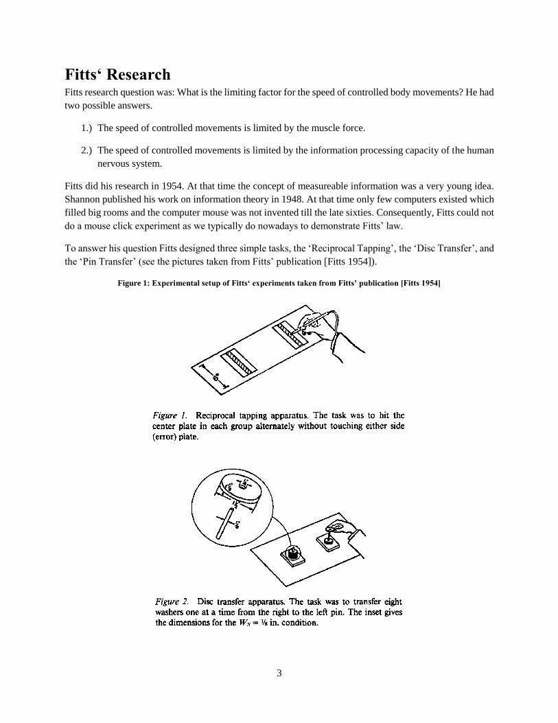
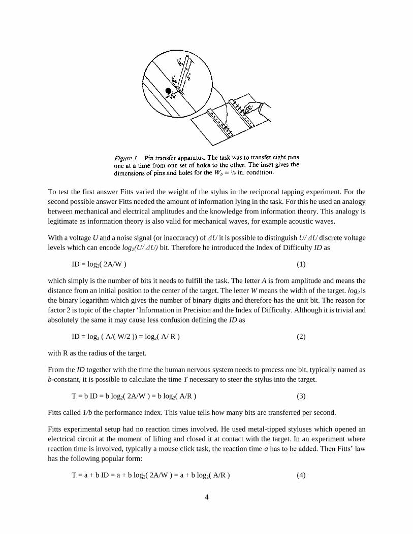
To answer his question Fitts designed three simple tasks, the ‘Reciprocal Tapping’, the ‘Disc Transfer’, and

the ‘Pin Transfer’ (see the pictures taken from Fitts’ publication [Fitts 1954]).

Figure 1: Experimental setup of Fitts‘ experiments taken from Fitts’ publication [Fitts 1954]

4

To test the first answer Fitts varied the weight of the stylus in the reciprocal tapping experiment. For the

second possible answer Fitts needed the amount of information lying in the task. For this he used an analogy

between mechanical and electrical amplitudes and the knowledge from information theory. This analogy is

legitimate as information theory is also valid for mechanical waves, for example acoustic waves.

With a voltage U and a noise signal (or inaccuracy) of ΔU it is possible to distinguish U/ ΔU discrete voltage

levels which can encode log2(U/ ΔU) bit. Therefore he introduced the Index of Difficulty ID as

ID = log2( 2A/W ) (1)

which simply is the number of bits it needs to fulfill the task. The letter A is from amplitude and means the

distance from an initial position to the center of the target. The letter W means the width of the target. log2 is

the binary logarithm which gives the number of binary digits and therefore has the unit bit. The reason for

factor 2 is topic of the chapter ‘Information in Precision and the Index of Difficulty. Although it is trivial and

absolutely the same it may cause less confusion defining the ID as

ID = log2 ( A/( W/2 )) = log2( A/ R ) (2)

with R as the radius of the target.

From the ID together with the time the human nervous system needs to process one bit, typically named as

b-constant, it is possible to calculate the time T necessary to steer the stylus into the target.

T = b ID = b log2( 2A/W ) = b log2( A/R ) (3)

Fitts called 1/b the performance index. This value tells how many bits are transferred per second.

Fitts experimental setup had no reaction times involved. He used metal-tipped styluses which opened an

electrical circuit at the moment of lifting and closed it at contact with the target. In an experiment where

reaction time is involved, typically a mouse click task, the reaction time a has to be added. Then Fitts’ law

has the following popular form:

T = a + b ID = a + b log2( 2A/W ) = a + b log2( A/R ) (4)

5

However, the a is never mentioned in Fitts’ paper.

The result of Fitts’ experiments was that the speed of the movement is not limited by the muscle force; the

subjects showed the same performance independent of the weight of the stylus. Instead the measured times

fitted to the concept of information processing.

ISO 9241-9 Beside the fact that the performance, or bit transfer, did not depend on the weight of the stylus, the bit

transfer was within 8 to 12 bits/second for all tasks. This means that the human nervous system has a general

limit for control tasks independent from the details of the task.

Therefore it is very surprising that the International Standardization Organization ISO defined the standard

ISO 9241-9 based on Fitts’ law to characterize the performance of input devices. Additionally, the ISO

9241-9 does not use the a- and b-constant but defines the throughput TP which merges both values to a

single one. There is a critical voice against the definition of TP [Zhai 2004]. However, it is questionable

whether the ISO standard makes sense at all.

Seeing the performance as a property of a device is the opposite of Fitts’ idea, who sees performance as a

property of the nervous system. Comparing a small laptop mouse against a big desktop mouse in the context

of a student exercise did not show differences in the performance. Comparing a trackball against a standard

mouse device typically shows that people perform better with the standard mouse device. However, people

who use a trackball for their daily work show the same performance with a trackball. This means the

performance on a pointing device depends on the subject and especially on her or his training on the device.

It seems that nobody uses the ISO-standard and manufacturers of mouse devices do not state a throughput

value for their products.

Exercise: Discuss the throughput TP for a mouse operated with the feet.

6

Information in Precision and the Index of Difficulty As mentioned already, at the time of Fitts’ research Shannon’s information theory was young and the

definition of the Index of Difficulty was difficult. Nowadays the meaning of bits is well known and the

relation of digits to precision is trivial – more digits allow higher precision. Every computer science student

knows that sending 10 bits to a plotter will position the plotter pen with a precision of 1/1024. If the amount

of information measured in bit is I, the precision p is 1/2I or

p = 2-I

(5)

Solved to I we get

I = log2 1/p (6)

If L is the length of the plotter’s range and W is the target size (diameter) or error interval, the precision p is

the ratio of the error interval and the plotter range:

p = W / L (7)

If the plotter arm is in the middle without any bit sent, the maximum distance to a target is half of the

plotter’s range and therefore A = L/2 or L = 2A. Putting this into the definition of precision (7) we get

p = W / 2A (8)

Putting this (8) into the formula (6) we get Fitts’ definition for the ID as in equation (1).

The factor 2 may be confusing but makes sense. It is the consequence that the precision p defines an interval

from -p/2 to +p/2 around the current position.

With no bit sent the plotter pen is in the middle and therefore already inside all targets which have their

center inside the plotter range and a radius of half the plotter range or a diameter of the plotter range,

respectively. With one bit sent we can position the plotter pen to the center of the left or right half and catch

all targets which are at least half plotter range in diameter. This is in accordance with Fitts’ definition of the

ID.

Fitts introduced the factor 2 with the words:

“The use of 2A rather than A is indicated by both logical and practical considerations. Its use insures that

the index will be greater than zero for all practical situations and has the effect of adding one bit (-log21/2)

per response to the difficulty index. The use of 2A makes the index correspond rationally to the number of

successive fractionations required to specify the tolerance range out of a total range extending from the

point of initiation of a movement to a point equidistant on the opposite side of the target.” [Fitts 1954, p.

267].

Perhaps Fitts did not express it in an elegant way and it sounds a little bit like passing the explanation he got

from an expert. Within the analogy to information theory, he mapped the amplitude of the noise to the width

of the target. However, the width of the target corresponds with the difference from peak to peak. In

consequence, he took also the peek-to-peek value for the amplitude of the movement, which is 2A (see

Figure 2).

7

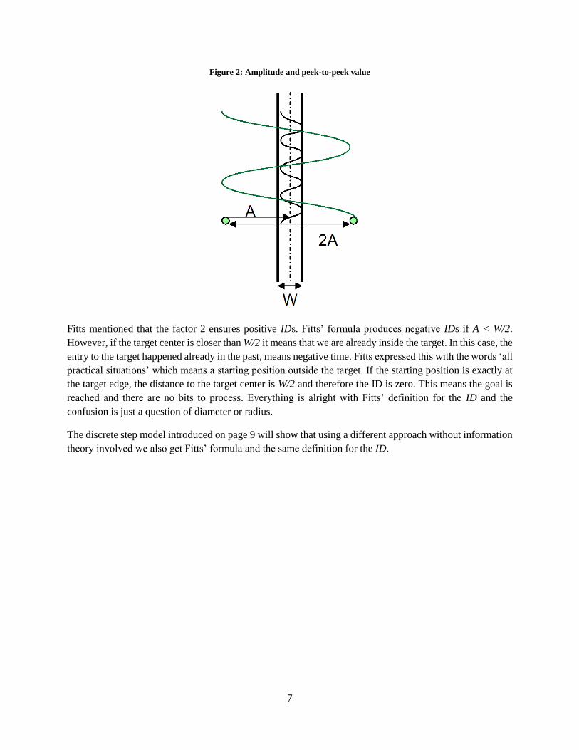
Figure 2: Amplitude and peek-to-peek value

Fitts mentioned that the factor 2 ensures positive IDs. Fitts’ formula produces negative IDs if A < W/2.

However, if the target center is closer than W/2 it means that we are already inside the target. In this case, the

entry to the target happened already in the past, means negative time. Fitts expressed this with the words ‘all

practical situations’ which means a starting position outside the target. If the starting position is exactly at

the target edge, the distance to the target center is W/2 and therefore the ID is zero. This means the goal is

reached and there are no bits to process. Everything is alright with Fitts’ definition for the ID and the

confusion is just a question of diameter or radius.

The discrete step model introduced on page 9 will show that using a different approach without information

theory involved we also get Fitts’ formula and the same definition for the ID.

8

Alternative Formulas for Fitts’ Law There are at least two additional formulas for Fitts’ law. One is known as Welford formulation:

T = a + b * log2 ( A/W + 0.5 ) (9)

The other formula is from MacKenzie who calls it Shannon formulation:

T = a + b * log2 ( A/W + 1 ) (10)

There is not much to find on the Internet about the Welford formulation; it is mostly printed matter.

MacKenzie, however, published his theory on the Internet (http://www.yorku.ca/mack/JMB89.html)

[MacKenzie 1989]. MacKenzie criticizes Fitts’ introduction of factor 2 to and argues that adding 1 instead

of multiplying with 2 will guarantee positive values for the ID. He refers to Shannon’s theorem 17, a

formula given as a footnote in Fitts’ publication, which has the desired +1 and then he does a ‘direct

analogy’ without further explanation. In his analogy the bandwidth (measured in bits/second) shall be

analog to time (measured in seconds) and power shall be analog to amplitude (power is proportional to the

square of the amplitude). There is no justification for such analogy.

MacKenzie’s formula became popular in HCI by his publication together with Sellen and Buxton

[MacKenzie, Sellen, Buxton 1991] and seems to be the most used Fitts’ law formula nowadays. However,

science is not a democracy.

It is impossible to prove with experimental data which formula is the right one. The differences in the

predicted times from the different formulas are small, especially if the distance A to the target is much bigger

than the target size W, which is normally the case. Additionally, Fitts’ law data are very noisy (have a look at

chapter ‘Evaluation of Fitts’ Law Data’). MacKenzie claims that his formula (10) shows better correlation

values for experimental data [MacKenzie 1989]. This seems to be true and is the reason for the chapter

‘Reality versus Model’. However, correlation does not tell much and the correlation gets even better if

adding 2 instead of 1 in formula (10).

Dropping the factor 2 in Fitts’ formula (4) does not affect the value of the b-constant. However, it affects

constant a.

T = a + b log2 ( 2A/W ) = a + b (log2 ( A/W ) + log2 2 ) = a + b + b log2 ( A/W )

= a’ + b log2 ( A/W ) (11)

with a’ = a + b (12)

This means that constant a’ does not have the meaning of reaction time anymore. Therefore some people

call the a’ -constant non-informal parameter, which contributes to the confusion.

It seems that there are more and more critical voices on the alternative formulas. The author of this lecture

raised the question which of the competing formulas is the right one [Drewes 2010]. Recently, Errol

Hoffmann managed to publish a critical paper [Hoffmann 2013] in the same journal where MacKenzie

published his theory. The best the HCI community can do is to ignore and forget the alternative formulas

and all research based upon.

9

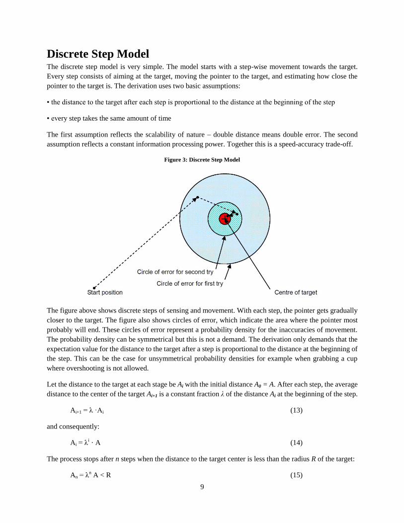
Discrete Step Model The discrete step model is very simple. The model starts with a step-wise movement towards the target.

Every step consists of aiming at the target, moving the pointer to the target, and estimating how close the

pointer to the target is. The derivation uses two basic assumptions:

• the distance to the target after each step is proportional to the distance at the beginning of the step

• every step takes the same amount of time

The first assumption reflects the scalability of nature – double distance means double error. The second

assumption reflects a constant information processing power. Together this is a speed-accuracy trade-off.

Figure 3: Discrete Step Model

The figure above shows discrete steps of sensing and movement. With each step, the pointer gets gradually

closer to the target. The figure also shows circles of error, which indicate the area where the pointer most

probably will end. These circles of error represent a probability density for the inaccuracies of movement.

The probability density can be symmetrical but this is not a demand. The derivation only demands that the

expectation value for the distance to the target after a step is proportional to the distance at the beginning of

the step. This can be the case for unsymmetrical probability densities for example when grabbing a cup

where overshooting is not allowed.

Let the distance to the target at each stage be Ai with the initial distance A0 = A. After each step, the average

distance to the center of the target Ai+1 is a constant fraction λ of the distance Ai at the beginning of the step.

Ai+1 = λ ·Ai (13)

and consequently:

Ai = λi · A (14)

The process stops after n steps when the distance to the target center is less than the radius R of the target:

An = λn A < R (15)

10

From this follows:

n = log2 ( R / A ) / log2 ( λ ) (16)

As it is possible to choose a logarithm with any basis we choose the binary logarithm log2.

Each step takes a fixed time τ. The total time T to reach the target is:

T = τ · n = τ log2 ( R /A ) / log2 ( λ ) (17)

T = b log2 ( A / R ) (18)

where b = - τ / log2 ( λ ). As the pointer gets closer to the target with each step, λ is smaller than 1 and

log2 ( λ ) is negative, so b is positive.

The formula derived from the discrete step model is exactly Fitts’ formula. Together with an some initial

time a for the brain to get started, means reaction time, we get the popular form

T = a + b log2 ( A / R ) (19)

Again we got Fitts’ formula (4) (and not one of the alternative formulas) and this time without information

theory and terms like ‘bits’ or ‘noise’.

11

Continuous Approach Model The problem with the discrete step model is it discreteness which does not allow describing the movement

on a continuous time scale (equation of motion). However, it is not very difficult to extend the discrete

model to a continuous model by making the steps smaller and finally doing an infinitesimal transition.

Let x(t) be the distance to the target center at time t and x(0) = A. In an infinitesimal time step dt the pointer

gets dx closer to the target. Together with the assumption that dx is proportional to the current distance x(t)

we get the equation

dx = c x(t) dt (20)

with c as the proportionality factor. Factor c is negative as we move towards the target at the origin of the

coordinate system. With a simple transformation

dx / dt = c x(t) (21)

we get a (very simple) differential equation, which is well-known from atomic decay or from discharging a

capacitor. The solution for the equation is an exponential function (e is the Euler number)

x(t) = A ect (22)

It is easy to see that x(0) = A and that x(t) tends towards zero when time goes towards infinity as c is

negative.

Of course it is possible to derive Fitts’ law from the equation of motion (22). When the pointer reaches the

target edge, the pointer is radius R (or half the width W/2) away from the target center. With T as the time to

reach the target we get the following equation

x(T) = A ecT

= R (23)

Solving this equation to T by drawing the logarithm we get

T = 1/c ln( R / A ) (24)

We transform this equation to

T = -1/c ln( A / R ) (25)

Together with ln x = log2 x / log2 e we can write

T = b log2 ( A / R ) (26)

with b = - 1 /( c * log2 e). This is again the formula (3) given by Fitts.

However, the reason to introduce the continuous approach model was not to derive Fitts’ formula a third

time. We will need the equation of motion for Figure 4 and equation (27) in the next chapter.

12

Reality versus Model In general it is desirable to have a model which predicts reality with high accuracy.

However, the accuracy is not the only criteria for a model. For any measured data it is possible to find a

formula, for example polynomials, which approximate the data quite well. In the eyes of an engineer such

empiric formula is valuable because it allows predicting accurate values. In the eyes of a scientist this

formula does not help much as it does not explain underlying mechanisms. Even if the accuracy is less,

scientist prefers a formula which was derived from assumptions. If measured data fit to the derived formula,

it is a strong hint that the assumptions are true. Even if an empiric formula produces better results because of

‘dirty effects’ not considered by the model assumptions, the derived formula brings more understanding.

Sometimes the benefit of a model lies in simplification. Typically, physicists derive formulas for a perfect

sphere rolling down a perfect plane. The resulting formula does not predict the motion of a real rock rolling

down a hill with high accuracy. However, the formula reflects concepts of translation-, rotation-, and

potential energies and allows general statements. A formula with the ambition to predict the motion of a real

rock rolling down a hill, if existing at all, would be so complex that it is questionable whether this formula is

of any value.

After this discussion on the value of models, we now have a look on the continuous model introduced above.

This model is a simplification and does not match reality perfectly. The main problem is the initial speed of

the movement.

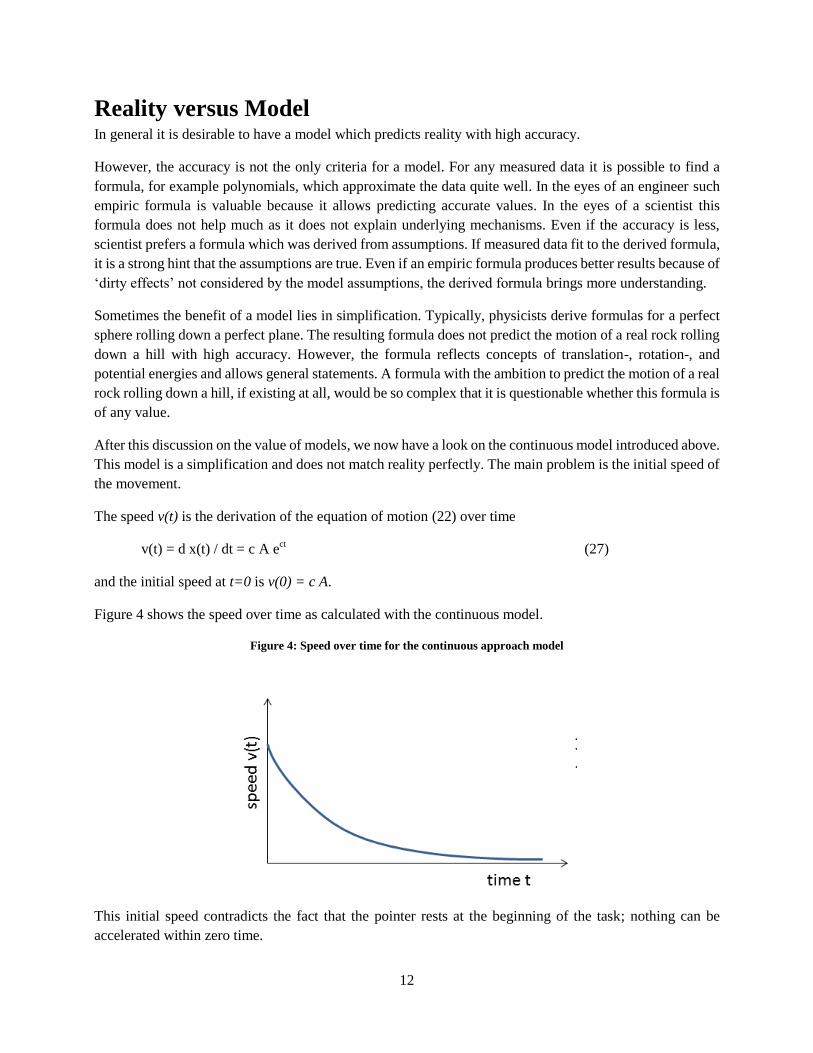
The speed v(t) is the derivation of the equation of motion (22) over time

v(t) = d x(t) / dt = c A ect (27)

and the initial speed at t=0 is v(0) = c A.

Figure 4 shows the speed over time as calculated with the continuous model.

Figure 4: Speed over time for the continuous approach model

This initial speed contradicts the fact that the pointer rests at the beginning of the task; nothing can be

accelerated within zero time.

13

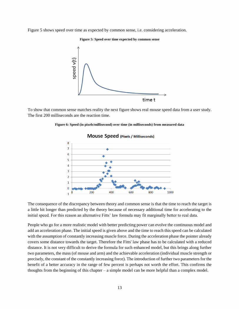
Figure 5 shows speed over time as expected by common sense, i.e. considering acceleration.

Figure 5: Speed over time expected by common sense

To show that common sense matches reality the next figure shows real mouse speed data from a user study.

The first 200 milliseconds are the reaction time.

Figure 6: Speed (in pixels/millisecond) over time (in milliseconds) from measured data

The consequence of the discrepancy between theory and common sense is that the time to reach the target is

a little bit longer than predicted by the theory because of necessary additional time for accelerating to the

initial speed. For this reason an alternative Fitts’ law formula may fit marginally better to real data.

People who go for a more realistic model with better predicting power can evolve the continuous model and

add an acceleration phase. The initial speed is given above and the time to reach this speed can be calculated

with the assumption of constantly increasing muscle force. During the acceleration phase the pointer already

covers some distance towards the target. Therefore the Fitts' law phase has to be calculated with a reduced

distance. It is not very difficult to derive the formula for such enhanced model, but this brings along further

two parameters, the mass (of mouse and arm) and the achievable acceleration (individual muscle strength or

precisely, the constant of the constantly increasing force). The introduction of further two parameters for the

benefit of a better accuracy in the range of few percent is perhaps not worth the effort. This confirms the

thoughts from the beginning of this chapter – a simple model can be more helpful than a complex model.

14

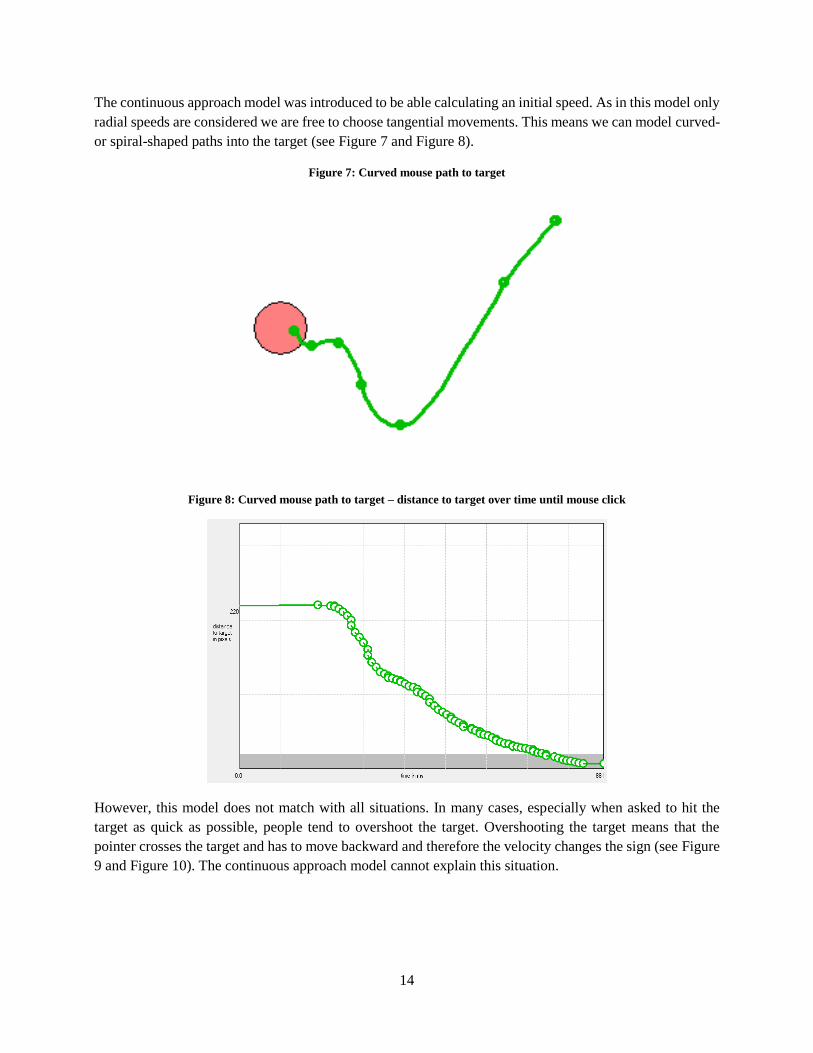
The continuous approach model was introduced to be able calculating an initial speed. As in this model only

radial speeds are considered we are free to choose tangential movements. This means we can model curved-

or spiral-shaped paths into the target (see Figure 7 and Figure 8).

Figure 7: Curved mouse path to target

Figure 8: Curved mouse path to target – distance to target over time until mouse click

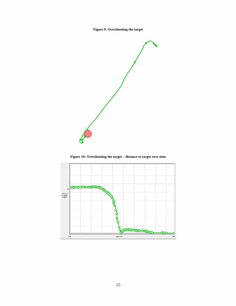
However, this model does not match with all situations. In many cases, especially when asked to hit the

target as quick as possible, people tend to overshoot the target. Overshooting the target means that the

pointer crosses the target and has to move backward and therefore the velocity changes the sign (see Figure

9 and Figure 10). The continuous approach model cannot explain this situation.

15

Figure 9: Overshooting the target

Figure 10: Overshooting the target – distance to target over time

16

Two- and Three-dimensional Movements and Target Shapes There is no reason to make the two- and three-dimensional case more difficult than it is. Looking at an

x-y-plotter it is clear that we have to transmit the double amount of information, e. g. bits, to a

two-dimensional plotter compared to a one-dimensional plotter. However, the positioning of the plotter pen

does not take the double time as typically both step motors work in parallel. The situation is the same for the

muscles of the human body. Every antagonistic pair of muscles is controlled by the nervous system which

needs b seconds processing a bit. This control processes take place in parallel and therefore the execution

time does not change with dimension. Fitts measured comparable values for the b-constant in the one- and

two-dimensional tasks. Also looking at the discrete step model makes clear that the dimensionality of the

task does not change the situation. The derivation of the discrete step model does not need any assumption

on the dimensionality; the math is the same for the one-, two-, and three-dimensional case.

One question of practical importance for the HCI community is the question on target shapes. Pointing on a

word, for example on a menu item, means that the target size differs on direction. Again the situation is quite

clear using common sense.

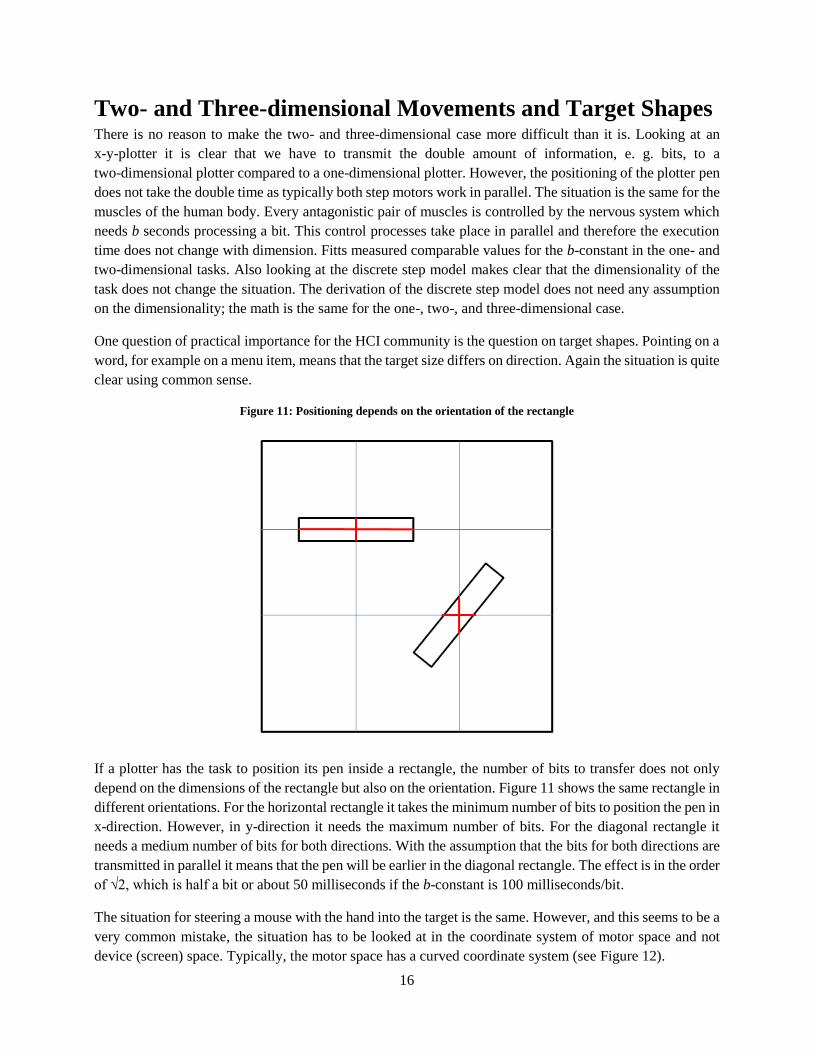
Figure 11: Positioning depends on the orientation of the rectangle

If a plotter has the task to position its pen inside a rectangle, the number of bits to transfer does not only

depend on the dimensions of the rectangle but also on the orientation. Figure 11 shows the same rectangle in

different orientations. For the horizontal rectangle it takes the minimum number of bits to position the pen in

x-direction. However, in y-direction it needs the maximum number of bits. For the diagonal rectangle it

needs a medium number of bits for both directions. With the assumption that the bits for both directions are

transmitted in parallel it means that the pen will be earlier in the diagonal rectangle. The effect is in the order

of √2, which is half a bit or about 50 milliseconds if the b-constant is 100 milliseconds/bit.

The situation for steering a mouse with the hand into the target is the same. However, and this seems to be a

very common mistake, the situation has to be looked at in the coordinate system of motor space and not

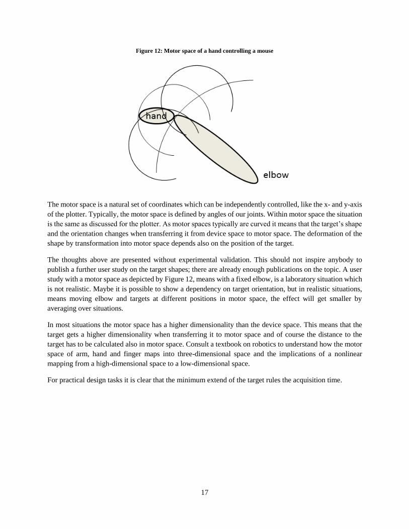
device (screen) space. Typically, the motor space has a curved coordinate system (see Figure 12).

17

Figure 12: Motor space of a hand controlling a mouse

The motor space is a natural set of coordinates which can be independently controlled, like the x- and y-axis

of the plotter. Typically, the motor space is defined by angles of our joints. Within motor space the situation

is the same as discussed for the plotter. As motor spaces typically are curved it means that the target’s shape

and the orientation changes when transferring it from device space to motor space. The deformation of the

shape by transformation into motor space depends also on the position of the target.

The thoughts above are presented without experimental validation. This should not inspire anybody to

publish a further user study on the target shapes; there are already enough publications on the topic. A user

study with a motor space as depicted by Figure 12, means with a fixed elbow, is a laboratory situation which

is not realistic. Maybe it is possible to show a dependency on target orientation, but in realistic situations,

means moving elbow and targets at different positions in motor space, the effect will get smaller by

averaging over situations.

In most situations the motor space has a higher dimensionality than the device space. This means that the

target gets a higher dimensionality when transferring it to motor space and of course the distance to the

target has to be calculated also in motor space. Consult a textbook on robotics to understand how the motor

space of arm, hand and finger maps into three-dimensional space and the implications of a nonlinear

mapping from a high-dimensional space to a low-dimensional space.

For practical design tasks it is clear that the minimum extend of the target rules the acquisition time.

18

Fitts’ Law Does not apply to Saccadic Eye Movements This chapter would not be necessary if there were not a handful of publications which did a Fitts’ law

evaluation for eye movements, for example [Ware, Mikaelian 1987], [Miniotas 2000], [Zhang, MacKenzie

2007], [Vertegaal 2008]. Psychology textbooks state that the eyes move ballistic, which is the opposite of

Fitts' law. Also Sibert and Jacob expressed themselves skeptical on the validity of Fitts’ law for the eyes

[Sibert, Jacob 2000].

Ballistic movements do not depend on target size. Psychology textbooks also give a formula for the time the

eyes need to position on a target. This formula was given by Carpenter [Carpenter 1977] and is independent

of target size

T = 21 ms + 2.2 ms/° · A (28)

A is the amplitude of the eye movement measured in degrees as the eye movement is a rotational movement.

Formula (28) assumes a linear relation (is a linear approximation) and was found by fitting with

experimental data. See Abrams, Meyer, and Kornblum [Abrams, Meyer, Kornblum 1989] for an eye speed

model assuming a constantly increasing eye muscle force which results in a cubic root relation. In both

approaches the eye movement time does not depend on a target size. It is hard to understand why some

publications in the field of HCI completely ignore the results of psychology and also do not even listen to

warning voices from their own community.

For clarifying the topic it is necessary to understand that the eye has two different types of movements

(beside movements on smaller scales like micro-saccades and drift and tremor). One type of eye movements

is compensation movements which compensate head movements or movements of the object looking at.

Such movements are smooth and may be controlled in a control-feedback loop. The other type of eye

movements is saccades, abrupt movements with speeds up to 700°/sec. This means that the visual

information on the retina changes quicker than the receptors can process and therefore the eye is virtually

blind during a saccade. This means that the movement cannot be controlled by a feedback loop and therefore

the movement is ballistic. The situation is comparable to throwing a stone; when the stone leaves the hand

there is no further control on the movement and the arrival at the target does not depend on the target size.

Assuming still that Fitts' law applies to eye movements is not only in contrast to the results of psychology

but also leaves open questions. The first thing which has to be discussed is the question whether target

acquisition by the eye is a single- or multi-saccade process. It seems that the eye is able to position on a

target with a single saccade with a precision which is enough to bring the target into the small field of high

resolution vision (fovea). The next thing to discuss is the target and its size. What are targets for the eye

when watching a video and what are the target sizes? When looking at a face what is the target - the eye, the

nose, the mouth or the whole face? However, without a target size it is impossible to calculate a time with

Fitts' formula.

19

Evaluation of Fitts’ Law Data Evaluating data needs some care and an understanding of the mathematical methods applied. The goal of the

evaluation is not to provide fantastic good value which impresses others, i.e. the reviewer of a submission.

The evaluation should be done with honesty.

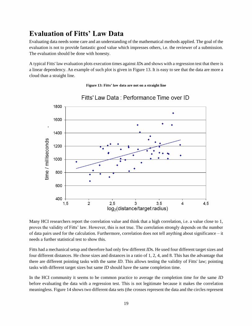
A typical Fitts' law evaluation plots execution times against IDs and shows with a regression test that there is

a linear dependency. An example of such plot is given in Figure 13. It is easy to see that the data are more a

cloud than a straight line.

Figure 13: Fitts’ law data are not on a straight line

Many HCI researchers report the correlation value and think that a high correlation, i.e. a value close to 1,

proves the validity of Fitts’ law. However, this is not true. The correlation strongly depends on the number

of data pairs used for the calculation. Furthermore, correlation does not tell anything about significance – it

needs a further statistical test to show this.

Fitts had a mechanical setup and therefore had only few different IDs. He used four different target sizes and

four different distances. He chose sizes and distances in a ratio of 1, 2, 4, and 8. This has the advantage that

there are different pointing tasks with the same ID. This allows testing the validity of Fitts' law; pointing

tasks with different target sizes but same ID should have the same completion time.

In the HCI community it seems to be common practice to average the completion time for the same ID

before evaluating the data with a regression test. This is not legitimate because it makes the correlation

meaningless. Figure 14 shows two different data sets (the crosses represent the data and the circles represent

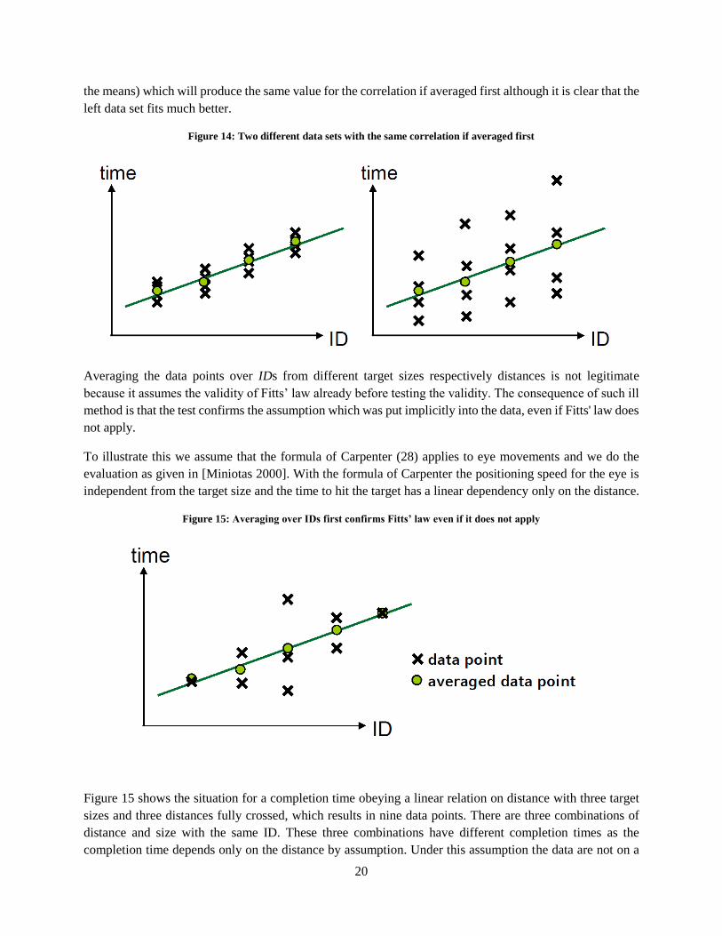
20

the means) which will produce the same value for the correlation if averaged first although it is clear that the

left data set fits much better.

Figure 14: Two different data sets with the same correlation if averaged first

Averaging the data points over IDs from different target sizes respectively distances is not legitimate

because it assumes the validity of Fitts’ law already before testing the validity. The consequence of such ill

method is that the test confirms the assumption which was put implicitly into the data, even if Fitts' law does

not apply.

To illustrate this we assume that the formula of Carpenter (28) applies to eye movements and we do the

evaluation as given in [Miniotas 2000]. With the formula of Carpenter the positioning speed for the eye is

independent from the target size and the time to hit the target has a linear dependency only on the distance.

Figure 15: Averaging over IDs first confirms Fitts’ law even if it does not apply

Figure 15 shows the situation for a completion time obeying a linear relation on distance with three target

sizes and three distances fully crossed, which results in nine data points. There are three combinations of

distance and size with the same ID. These three combinations have different completion times as the

completion time depends only on the distance by assumption. Under this assumption the data are not on a

21

straight line, but the averaged data are and a regression test on the five averaged data produces a ‘very good’

correlation. By the way, even a regression test on the nine raw data delivers a correlation above zero and

indicates a linear dependency.

As there are many publications proving Fitts’ law with data averaged over ID first, the topic seems to be

important. Therefore an example, which everybody can reproduce with a standard spreadsheet application,

follows.

Let us assume a linear dependency for the completion time, which only depends on the distance and not on

the size of the target. We will get a correlation close to 1 although we explicitly assume that Fitts’ law does

not apply.

For convenience of an easy calculation the target sizes and distances are 1, 2, 4, and 8 in arbitrary and

perhaps different units. This is legitimate because the correlation is independent from scales. People who are

not familiar with the math can use concrete target sizes in centimeter or inch and calculate concrete times

from a linear formula; they will get the same results.

Typical Fitts’ law user studies use four target sizes with the ratios 1, 2, 4 and 8 and four distances with the

same ratios. This results in seven different ratios of distance and target size as shown in Table 1.

Table 1: All combinations for four distances A and four target radius R

A/R 1 2 4 8

1 1 2 4 8

2 1/2 1 2 4

4 1/4 1/2 1 2

8 1/8 1/4 1/2 1

Typically, the subjects in such a user study perform positioning tasks over all combinations of target sizes

and distances, which results in data probes of uniform distribution over all combinations. With a linear

relation it is possible to calculate the average execution time from the average distance. Table 2 shows all

possible IDs and the resulting average distances ( ∑ A / # ).

Table 2: All possible IDs and the corresponding average distance

A/R log2(A/R) # ∑ A ∑ A / #

1/8 -3 1 1 1

1/4 -2 2 1+2 3/2

1/2 -1 3 1+2+4 7/3

1 0 4 1+2+4+8 15/4

2 1 3 2+4+8 14/3

4 2 2 4+8 6

8 3 1 8 8

Figure 16 shows the average distance over ID as given in Table 2 (circles) together with their trend line

(solid) and all 16 data (crosses) according to Table 1 also together with their trend line (dashed). The

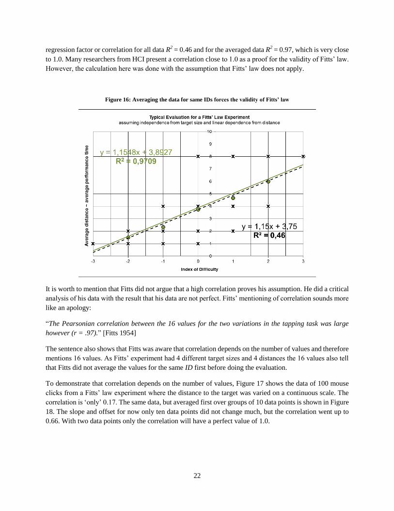
22

regression factor or correlation for all data R2 = 0.46 and for the averaged data R

2 = 0.97, which is very close

to 1.0. Many researchers from HCI present a correlation close to 1.0 as a proof for the validity of Fitts’ law.

However, the calculation here was done with the assumption that Fitts’ law does not apply.

Figure 16: Averaging the data for same IDs forces the validity of Fitts’ law

It is worth to mention that Fitts did not argue that a high correlation proves his assumption. He did a critical

analysis of his data with the result that his data are not perfect. Fitts’ mentioning of correlation sounds more

like an apology:

“The Pearsonian correlation between the 16 values for the two variations in the tapping task was large

however (r = .97).” [Fitts 1954]

The sentence also shows that Fitts was aware that correlation depends on the number of values and therefore

mentions 16 values. As Fitts’ experiment had 4 different target sizes and 4 distances the 16 values also tell

that Fitts did not average the values for the same ID first before doing the evaluation.

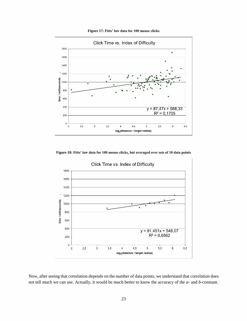
To demonstrate that correlation depends on the number of values, Figure 17 shows the data of 100 mouse

clicks from a Fitts’ law experiment where the distance to the target was varied on a continuous scale. The

correlation is ‘only’ 0.17. The same data, but averaged first over groups of 10 data points is shown in Figure

18. The slope and offset for now only ten data points did not change much, but the correlation went up to

0.66. With two data points only the correlation will have a perfect value of 1.0.

23

Figure 17: Fitts’ law data for 100 mouse clicks

Figure 18: Fitts’ law data for 100 mouse clicks, but averaged over sets of 10 data points

Now, after seeing that correlation depends on the number of data points, we understand that correlation does

not tell much we can use. Actually, it would be much better to know the accuracy of the a- and b-constant.

24

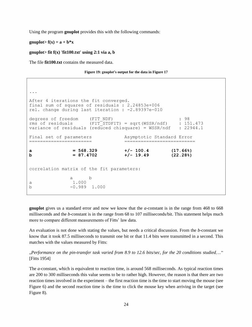
Using the program gnuplot provides this with the following commands:

gnuplot> f(x) = a + b*x

gnuplot> fit f(x) 'fit100.txt' using 2:1 via a, b

The file fit100.txt contains the measured data.

Figure 19: gnuplot’s output for the data in Figure 17

...

After 4 iterations the fit converged.

final sum of squares of residuals : 2.24853e+006 rel. change during last iteration : -2.89397e-010

degrees of freedom (FIT_NDF) : 98 rms of residuals (FIT_STDFIT) = sqrt(WSSR/ndf) : 151.473

variance of residuals (reduced chisquare) = WSSR/ndf : 22944.1

Final set of parameters Asymptotic Standard Error

======================= ==========================

a = 568.329 +/- 100.4 (17.66%) b = 87.4702 +/- 19.49 (22.28%)

correlation matrix of the fit parameters:

a b

a 1.000

b -0.989 1.000

gnuplot gives us a standard error and now we know that the a-constant is in the range from 468 to 668

milliseconds and the b-constant is in the range from 68 to 107 milliseconds/bit. This statement helps much

more to compare different measurements of Fitts’ law data.

An evaluation is not done with stating the values, but needs a critical discussion. From the b-constant we

know that it took 87.5 milliseconds to transmit one bit or that 11.4 bits were transmitted in a second. This

matches with the values measured by Fitts:

„Performance on the pin-transfer task varied from 8.9 to 12.6 bits/sec, for the 20 conditions studied,…“

[Fitts 1954]

The a-constant, which is equivalent to reaction time, is around 568 milliseconds. As typical reaction times

are 200 to 300 milliseconds this value seems to be to rather high. However, the reason is that there are two

reaction times involved in the experiment – the first reaction time is the time to start moving the mouse (see

Figure 6) and the second reaction time is the time to click the mouse key when arriving in the target (see

Figure 8).

25

The discussion of the results shows, that the evaluation of the presented Fitts’ law experiment is in

accordance with the research of Fitts and that the results are plausible.

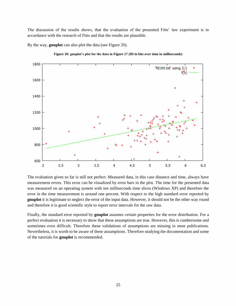
By the way, gnuplot can also plot the data (see Figure 20).

Figure 20: gnuplot’s plot for the data in Figure 17 (ID in bits over time in milliseconds)

The evaluation given so far is still not perfect. Measured data, in this case distance and time, always have

measurement errors. This error can be visualized by error bars in the plot. The time for the presented data

was measured on an operating system with ten milliseconds time slices (Windows XP) and therefore the

error in the time measurement is around one percent. With respect to the high standard error reported by

gnuplot it is legitimate to neglect the error of the input data. However, it should not be the other way round

and therefore it is good scientific style to report error intervals for the raw data.

Finally, the standard error reported by gnuplot assumes certain properties for the error distribution. For a

perfect evaluation it is necessary to show that these assumptions are true. However, this is cumbersome and

sometimes even difficult. Therefore these validations of assumptions are missing in most publications.

Nevertheless, it is worth to be aware of these assumptions. Therefore studying the documentation and some

of the tutorials for gnuplot is recommended.

26

Steering Law One valuable extension to Fitts’ law from the HCI community is the steering law of Accot and Zhai [Accot,

Zhai 1997]. The idea behind the steering law is that steering a vehicle through a narrow tunnel needs more

time than steering it through a wide tunnel. The same is true for steering the mouse through cascading

menus.

The question for the steering law is: How much time does it need to steer the mouse through a tunnel of

length A (A stands for amplitude to be consistent with Fitts’ law) and width W?

One possible approach is a model with a speed-accuracy trade-off similar to the discrete step model. A

movement within one time unit can be short or long, but the accuracy of the movement is a fraction of the

covered length. The maximum movement within one time unit is a movement where the error circle does

not exceed the width of the tunnel.

Figure 21: Steering through a tunnel

For simplicity we assume a straight tunnel of constant width W. Let f be the factor to calculate the radius of

the error circle from the length of the movement:

r = f s (29)

For not bumping into the borders of the tunnel the error circle has to be smaller than the width of the tunnel:

r < W/2 (30)

Together with the relation of distance and error (29) and an equal sign for the maximum distance we get

f s = W / 2 (31)

and solved for s:

s = W / ( 2 f ) (32)

Now it is easy to calculate the time T for steering through a tunnel of length A and width W. As we move

distance s in one time unit we have to divide the total length by s:

T = 2 f A / W (33)

27

This formula is the same as given by Accot and Zhai, however derived from different assumptions and with

simpler math.

The approach of Accot and Zhai has a severe problem. They divide the steering task into n subtasks of Fitts’

law-type with tunnel length A/n and do an infinitesimal transition using MacKenzie’s formula.

IDtunnel = n * log2( A/(nW) + 1 ) = log2( A/(nW) + 1 )n (34)

The argument of the logarithm is a well-known series (the limit definition of the exponential function eA/W

by Euler). The problem is that with Fitts’ correct formula, means without the 1, the infinitesimal transition

does not converge. Therefore it is doubtful whether it is possible to compose a steering task from infinite

small Fitts’ law-type tasks.

The derived formula (33) shows that the travelling time T is proportional to the length A of the tunnel. This

is what we expect by common sense. If we know the time it needs to steer through a certain tunnel, we can

connect the same tunnel at the end of the first tunnel and the traveling time will be double. Concatenating n

tunnels with traveling times ti will result in a traveling time which is the sum of all ti. If the tunnel has

changing widths it is possible to divide the tunnel into pieces with constant width and sum the times for the

pieces. This gave Accot and Zhai the idea to calculate the steering time for a tunnel with changing widths

from a path integral. They also proposed to calculate complex paths, means curved paths, by integration

over the curvilinear abscissa.

IDtunnel = ∫

(35)

This is a very elegant way to express it and may work in ‘nice’ conditions, but goes much too far. It ignores

that there is something like a characteristic length (the s in Figure 21) which prohibits an infinitesimal

transition. Strictly speaking it is a characteristic ratio (the f in formula (29)) as the geometry is free of scale.

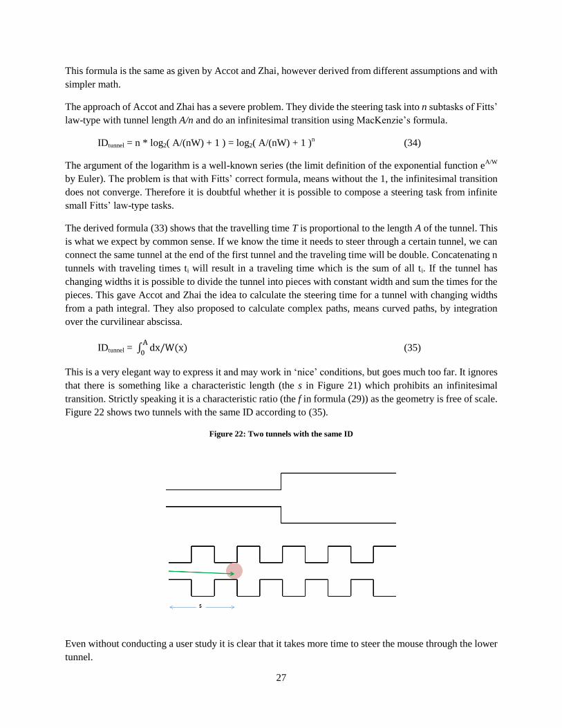
Figure 22 shows two tunnels with the same ID according to (35).

Figure 22: Two tunnels with the same ID

Even without conducting a user study it is clear that it takes more time to steer the mouse through the lower

tunnel.

28

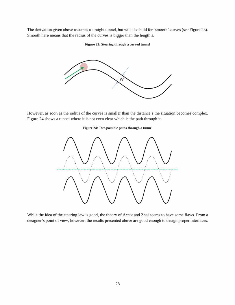
The derivation given above assumes a straight tunnel, but will also hold for ‘smooth’ curves (see Figure 23).

Smooth here means that the radius of the curves is bigger than the length s.

Figure 23: Steering through a curved tunnel

However, as soon as the radius of the curves is smaller than the distance s the situation becomes complex.

Figure 24 shows a tunnel where it is not even clear which is the path through it.

Figure 24: Two possible paths through a tunnel

While the idea of the steering law is good, the theory of Accot and Zhai seems to have some flaws. From a

designer’s point of view, however, the results presented above are good enough to design proper interfaces.

29

Recommendations for Fitts’ Law Researchers There are already many publications on Fitts' law, perhaps already too much. Anybody who intends to

publish papers on Fitts' law should make sure it is a relevant publication. Researchers should not mention

Fitts’ law, just for making their publication ‘more scientific’.

Fitts’ law researcher should also have the necessary math background. The math of information theory is

not trivial and the evaluation of data needs good statistics knowledge. Modern software, for example a

spreadsheet application, make complex math available to everybody. The software has no awareness

whether the math makes sense for the particular data and calculates a result. With respect to Fitts’ law it

means that a spreadsheet application calculates a regression line and a correlation, even if the person who

entered the data has no idea what the meaning of correlation is.

However, putting impressive formulas into a publication to make it look scientific will not make it scientific.

It is also not true that things have to be difficult or need complex math to be scientific. Actually, good

science prefers simplicity and common sense.

A scientific approach has methodology. Measuring data in a user study, processing the data with a math

software package and proudly present values is not scientific. First we need an assumption or model from

which we can derive a prediction. Then we measure data in a user study. After the evaluation of the data we

have to discuss the results and compare it with the predictions we made. If the results do not match with the

prediction our assumptions or model is wrong. However, if the results match the predictions it means that

the assumptions might be true.

Additionally, a researcher should know the state of the art. Regarding the research done in the HCI

community this is a lot of work because of the big number of publications. Most publications on Fitts’ law

done by the HCI community refer to very old results from psychology and mostly to other HCI publications.

Fitts published his paper in 1954. For science this is very long time ago and there was most probable some

progress in the field. Fitts was a psychologist and it is very likely that other psychologists continued the

research in the fifties and sixties; finally, psychologists also like to publish. Maybe it is difficult finding this

research because it is printed matter and not available as a PDF document on internet search engines.

However, it seems that there are no recent research results for Fitts’ law in psychology, which means that

psychology does not research Fiits’ law anymore.

Most probably the reason is that nowadays the message of Fitts is well understood. Typically, science

researches something until it is understood and after it starts to research something else. HCI does Fitts’ law

research now for nearly three decades and therefore a publication on Fitts’ law from the HCI community

should aim for final understanding.

Shannon’s theory explains transmission of bits. It does not really explain processing of bits. Therefore

theories based on Shannon’s theory have limitations in the understanding. Fitts’ law explains quite well why

it takes more time to hit a smaller target, but it does not explain the high variance in performance time. There

was so much progress in science since the times of Fitts and perhaps it is time for new concepts. How do

neural networks perform when controlling a pointing task? What do people who build robots know about the

topic?

30

Meaning of Fitts’ Law for HCI The practical meaning of Fitts’ law for the HCI community was explained in the preface – it takes more time

to hit a target if it is further away or smaller. There is no reason making a big deal of it and it is definitely not

worth the several hundred publications on the topic. Fights for the most exact formula predicting target

acquisition times do not bring any benefit and have no implication on practical design issues.

Fitts’ law experiments suit perfectly for student exercises. The software is easy to program on any platform,

the user study does not take much time, and the measured data are the base for exercising statistical

methods. There are many pointing devices, mouse devices, trackballs, touchpads and joysticks, which allow

many variations for a different exercise in the next course.

Of course the concept of limited information transmission from a human to a device has relevance for

human computer interaction. Therefore it seems natural that the HCI community does research on this topic.

However, the concept is well-known for more than half a century and there was a lot of psycho-motor

research done already and therefore the concept is also well-understood, at least outside HCI.

It seems that the motivation for Fitts’ law research by the HCI community is the scientific claim. Fitts’

formula is the only non-trivial formula in HCI and has a relation to Shannon’s information theory which is

definitely hard science. Therefore Fitts’ law could support the scientific claim of a community which mostly

deals with soft design issues. However, if people do research on a naïve level it can also prove the opposite.

31

References [Abrams, Meyer, Kornblum 1989] Abrams R.A., Meyer D.E., Kornblum, S. Speed and Accuracy of

Saccadic Eye Movements: Characteristics of Impulse Variability in the Oculomotor System. Journal

of Experimental Psychology: Human Perception and Performance (1989), Vol. 15, No. 3, 529 – 543.

(http://www-personal.umich.edu/~kornblum/files/journal_exp_psych_HPP_15-3.pdf)

[Accot, Zhai 1997] Accot J., Zhai S. Beyond Fitts' law: models for trajectory-based HCI tasks. In CHI '97.

ACM Press (1997), 295-302.

[Carpenter 1977] Carpenter, R. H. S. Movement of the Eyes, London: Pion (1977)

[Drewes 2010] Drewes, H. Only one Fitts' law formula please! In Extended Abstracts CHI EA '10. ACM

Press (2010), 2813 – 2822.

(http://www.medien.ifi.lmu.de/pubdb/publications/pub/drewes2010chi/drewes2010chi.pdf)

[Fitts 1954] Fitts, P. M. The Information Capacity of the Human Motor System in Controlling the

Amplitude of Movement, In Journal of Experimental Psychology (1954), 47, 381 – 391.

(http://e.guigon.free.fr/rsc/article/Fitts54.pdf)

[Hoffmann 2013] Hoffmann, E. R. Which Version/Variation of Fitts’ Law? A Critique of

Information-Theory Models. In Journal of Motor Behavior (2013), Volume 45, Issue 3, p. 205-215.

[MacKenzie 1989] MacKenzie, I. S. A Note on the Information-Theoretic Basis for Fitts' Law. In Journal of

Motor Behavior (1989), 21, 323 – 330. (http://www.yorku.ca/mack/JMB89.html)

[MacKenzie, Sellen, Buxton 1991] MacKenzie, I. S., Sellen, A., Buxton, W. A. A comparison of input

devices in element pointing and dragging tasks. In CHI '91. ACM Press (1991), 161 – 166.

[Miniotas 2000] Miniotas, D. Application of Fitts' Law to Eye Gaze Interaction. In Extended Abstracts

CHI '00. ACM Press (2000), 339 – 340.

[Sibert, Jacob 2000] Sibert, L. E., Jacob, R. J. Evaluation of Eye Gaze Interaction. In CHI '00. ACM Press

(2000), 281 – 288. (http://www.cs.tufts.edu/~jacob/papers/chi00.sibert.pdf)

[Vertegaal 2008] Vertegaal, R. A Fitts Law comparison of eye tracking and manual input in the selection of

visual targets. Conference on Multimodal interfaces IMCI '08. ACM (2008.) 241 – 248.

[Ware, Mikaelian 1987] Ware, C., and Mikaelian, H. H. An Evaluation of an Eye Tracker as a Device for

Computer Input. In CHI '87. ACM Press (1987), 183 – 188

[Zhai 2004] Zhai, S. Characterizing computer input with Fitts' law parameters – The information and

non-information aspects of pointing. Int. J. Hum.-Comput. Stud. 61, 6 (2004), 791 – 809.

(http://www.almaden.ibm.com/u/zhai/papers/FittsThroughputFinalManuscript.pdf)

[Zhang, MacKenzie 2007] Zhang, X., MacKenzie, I. S. Evaluating Eye Tracking with ISO 9241 – Part 9.

HCI International 2007, Heidelberg: Springer (2007), 779 – 788.

(http://www.yorku.ca/mack/hcii2007.html)