A human system learning model for solving the inverse kinematics problem by direct inverse modeling

Systems and Computers in Japan, Vol. 27, No. 8, 1996 Translated from Denshi Joho Tsushin Gakkai Ronbunshi, Vol. J78-D-11, No. 9, September 1995, pp. 1383-1394

A Human System Learning Model for Solving the Inverse Kinematics Problem by Direct Inverse Modeling

Eimei Oyama

Mechanical Engineering Laboratory, Tsukuba, Japan 305

Taro Maeda and Susumu Tachi

Faculty of Engineering, The University of Tokyo, Bunkyo, Tokyo, Japan 113

SUMMARY

The problem of computing a human arm posture that will take the hand to a desired hand position given by vision is called an inverse kinematics problem. To solve this problem, the human nervous system has a system for solving the inverse kinematics problem computing the proper joint angles from the desired hand position.

Although the direct inverse modeling method is popular for the acquisition of an inverse kinematics model, a sufficient inverse model cannot be obtained for such systems with many-to-one input-output correspondence as a human arm system.

This paper, proposes a new model of a human inverse kinematics solver which uses the learned inverse model of the linearized model of the human arm. This inverse model transforms the hand position error to the update vector of the joint angles. The solver inverse kinematics problems by using the hand position error feedback. The performance of the solver is shown using numerical simulations.

Key words: Human hand position; control learning; inverse kinematics neural networks, direct inverse modeling; output feedback inverse model.

1. Introduction

The problem of computing a human arm posture that will take the human hand to a desired position given by vision is a kind of inverse problem. In order to solve the problem, an inverse kinematics solver, i.e., a system for solving an inverse kinematics problem, computing the proper joint angles from the desired hand position is necessary. A human forms the solver in the human nervous system. How the human nervous system acquires the inverse kinematics solver is one of the important problems in neuroscience. Al- though some theoretical models were proposed, they have a number of drawbacks.

A representative model of the solver solves inverse kinematics problems by using a learned inverse kinematics model which calculates a joint angle vector that corresponds to the hand position.

A representative inverse kinematics model learning method employed by many researchers uses a target systems output as input to the inverse model can uses the target systems input as the teaching signal of the inverse kinematics model that is composed of a learning element. This method called Direct Inverse Modeling (DIM) by Jordan [l]. Kuperstein [2] and Sakaguchi [3] proposed a model of a human inverse

53 ISSN0082- 1666/96/0008-0053 1996 Scripta Technica, Inc.

kinematics solver that uses an inverse kinematics model learned by DIM. However, a sufficient inverse model cannot be obtained by DIM when the correspondence between the input and the output of the target system is not one-to-one and is nonlinear [ 11. There are many joint angle vectors that correspond to one desired hand position. The inverse kinematics problem of a human arm is an ill-posed problem and cannot be solved by an inverse kinematics model learned by DIM.

In this paper, we propose a new learning model of the inverse kinematics solver that avoids the ill- posedness of the inverse kinematics problem by a modification of the target system. The relationship between the infinitesimal change of the joint angle vector and that of the hand position vector is linear. A kind of inverse kinematics model which transforms the desired change of the hand position to the update vector of the joint angles can be obtained by using DIM. The proposed inverse kinematicssoker uses the acquired inverse model of the linearized model of the human arm as a hand position error feedback system and finds an inverse kinematics solution through iterative improvement.

The performance of the proposed method is shown by numerical simulations. At this stage, the proposed learning model still has some problems. However, the model can solve inverse kinematicsprob- lems of redundant arms. It can be a basic model of human inverse kinematics solver for discussion.

2. A Model of Human Hand Position Control System

2.1. Formulation of problem

Let x be a n x 1 hand position vector given by the vision system and # be a m X 1 vector of joint angle vector. The relationship between x and 8 is expressed as

where f is a C' class function. When a desired hand position vector xd is given, consider an inverse kinematics problem that calculates the joint angle vector 8 , that satisfies

x d = f (6,) (2)

f is C' class function. Assume that an ideal learning element can approximate any continuous function. When the input of the learning element is t , let 4(t) be

the output of the element and 4 ( t ) be the teaching signal for the learning element. After teaching signals sj (j = 1,2,3, ...) are given for the learning element as

U( t )=s j (3)

then

@( t 1 + E(sj) (4)

is established;E(s,) is the mean of s j ; and 4@) is a C' class function. J3y the generalization function of the learning element, 4(t) learned at representative points t i (i = 1, 2, 3, ...) in the input space t can generate correct outputs at the whole input space 1.

Representative learning elements, for example, the multilayer neural networks learned through backpropagation learning [4], Albus' CMAC [S], and Ko- honen's topographic mapping networks 161 satisfy Eq. (4) approximately.

2.2. Assumption about human inverse Linema- tics solver

Kawato et al. proposed the hierarchical information processing model of the human voluntary movement [7l. The model consists of the following three information processings: (I) trajectory planning in the visual coordinates; (11) transformation of the trajectory from visual coordinates to body coordinates; and (111) control that generates motor commands to realize the desired trajectory.

In this paper, (11) coordinate transformation is considered. When a target point in the visual place is given, a human can move the hand to the point pre- cisely by use of visual feedback. On the other hand, the precision of the hand position is greatly deteri- orated without the viewing of the hand [8]. Consider- ing these facts, the possibility is only slight that the human inverse kinematics solver depends mainly on the relationship between the absolute hand position in the visual coordinates and the absolute kinesthetic information. Since the measurement precision of the relative position and the change of the position is high [9-111, we assume that the human inverse kinematics solver is based on the relationship between the change of the hand position vector in the visual coordinates and the change of the joint angle vector in the body coordinates. Kawato proposed a learning model that acquires the Moore-Penrose Inverse of the Jacobian of the human arm for coordinate transformation by using the relationship between the vector of the change of

54

the hand position and that of the joint angle vector [ 121. However, since this learning model uses a complex adaptive rule based on the steepest descent method, it has a drawback as a model of a human nervous system.

Georgepoulos et al. found neurons in the motor cortex of a rhesus monkey that become active at high firing rate when the monkey moves its hand in a certain direction [13-151. A population vector is defined as the weighted sum of the peculiar direction of the neuron. The weight is calculated based on the difference between the current firing rate of the corresponding neuron and the firing rate at rest. The population vector predicted accurately the direction of the hand movement. The length of the vector has a strong relationship to the hand velocities. It is found that the firing rates of these direction-sensitiveneurons in the motor cortex changes as the starting point of the hand changes [ 161.

Anderson et al. found the neurons which encode the position of the visual target on the head coordinates in the parietal association cortex [ 171. Gentilucci et al. found target-sensitive neurons in inferior pre- motor cortex [ 181. There are some developed models and objections regarding Georgopoulos’ model [ 19-20]. However, there are neurons that have strong relation- ships to the direction of the hand movement in the parietal association cortex, the frontal association cortex, and the primary motor cortex. The primary motor cortex generates motor command based on the body coordinates [21]. The coordinate transformation system from the visual coordinates to the body coordinates must exist in these areas.

The vector of the change of the hand position or that of the velocity of the hand position has the same direction as the direction of the hand movement. From the physiological viewpoint, the change of the hand position is important in the human hand position control. Since the active area of the motor cortex changes according to the initial posture of the arm, the joint angle vector also is an important information.

Let 8 be the joint angle vector, xd be the desired hand position vector, h d be the desired change of the hand position vector, and &d be the desired change of the joint angle vector. In this paper, a learning model of the human inverse kinematics solver that transforms h d to &d and generates the position command of the joint angles sequentially is proposed.

It is clear that a human has an inverse kinematics

model that is based on the relationship of the absolute hand position and the absolute joint angle vector and transforms the desired hand position to the joint angles command directly. This type of inverse kinematics model is not considered in this paper. After acquisition of the visual feedback system stated in section 2.3, the inverse kinematics model can be obtained by feedback error learning scheme proposed by Kawato [7].

23. Output feedback inverse model

Bullock and Grossberg proposed a computational model of the human arm control system that can ex- plain Georgopoulos’ experimental results [22]. By using the error vector between the final goal of the hand position xde and the hand position x at the time f is defined as

the desired hand position q ( t ) is updated sequentially. If x(t) is controlled successfully to track the desired hand position xd(t), the direction of e(f) is constant in the reaching motion. Thus, Bullock and Grossberg asserted that Georgopoulos’ results are explained.

We assume also that the desired trajectory is calculated in the visual coordinates and the temporal desired hand position is calculated sequentially at each time of the motion.

Hereafter, we use discrete descriptions for modeling of the human motion control system.

Let At be the sampling interval; tk refers to the time k h . Hereafter, vector y(k) refers to the value of the vectory at time f k . The sampling interval At is set to 0.1-0.3 s that corresponds to the time delay between the visual stimulus and the start of the visually guided motion.

The change of the desired hand position is calculated as

The hand position error is calculated as

The desired change of the hand position including the output error feedback is calculated as

55

where K is an appropriate coefficient.

Let Md(k) be the update vector of the joint angle vector that will correspond to the desired change of the hand position Av’Ak). By updating the joint angle vector as

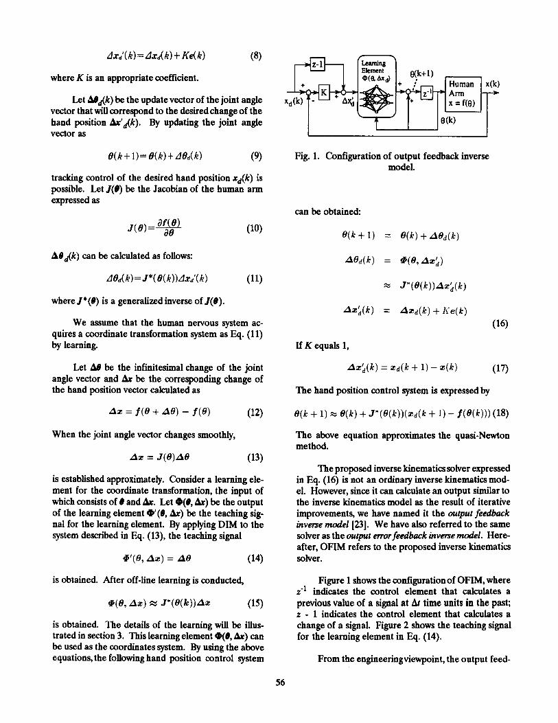
i Fig. 1. Configuration of output feedback inverse

model. tracking control of the desired hand position xd(k) is possible. Let J(8) be the Jacobian of the human arm expressed as

can be obtained

A#&) can be calculated as follows:

where J’(8) is a generalized inverse of J(8).

We assume that the human nervous system acquires a coordinate transformation system as Eq. (1 1) by learning.

Let A4 be the infinitesimal change of the joint angle vector and Ar be the corresponding change of the hand position vector calculated as

When the joint angle vector changes smoothly,

is established approximately. Consider a learning element for the coordinate transformation, the input of which consists of 8 and br. Let @((I, Ar) be the output of the learning element W(#, Ar) be the teaching signal for the learning element. By applying DIM to the system described in Eq. (13), the teaching signal

@‘(8, A z ) = A 8 (14)

is obtained. After off-line learning is conducted,

@(8, A z ) x J*(8 (k ) )Az (15)

is obtained. The details of the learning will be illus- trated in section 3. This learning element 4(8, Ar) can be used as the coordinates system. By using the above equations, the following hand position control system

If K equals 1,

The hand position control system is expressed by

The above equation approximates the quasi-Newton method.

The proposed inverse kinematics solver expressed in Eq. (16) is not an ordinary inverse kinematics model. However, since it can calculate an output similar to the inverse kinematics model as the result of iterative improvements, we have named it the output feedback inverse model [23]. We have also referred to the same solver as the output error feedback inverse model. Here- after, OFIM refers to the proposed inverse kinematics solver.

Figure 1 shows the configuration of OFIM, where 2-l indicates the control element that calculates a previous value of a signal at At time units in the past: z - 1 indicates the control element that calculates a change of a signal. Figure 2 shows the teaching signal for the learning element in Eq. (14).

From the engineeringviewpoint, the output feed-

56

Fig. 2. Teaching signal for learning element.

back inverse model does not have sufficient precision and usually requires a long learning time. Kawato’s learning method of a nonlinear feedback gain or our improved model for engineering application can be useful for practical application [7, 241.

2.4. Coordinate transformation system paying attention to velocity and acceleration

The relationship between the velocity vector of the joint angles and that of the hand position

s = J ( e ) e (19)

is linear as well as Eq. (13). An inverse model of the system as described in Eq. (19) can also be obtained by DIM.

The relationship between the acceleration vector of the joint angles and that of the hand position

In order toe calculate the joint angle vector that corresponds to the fixed desired hand position, first, an initial joint angle vector is generated and a trajectory that continuously connects the initial hand position and the fixed desired hand position is calculated. Then, by tracking the trajectory, OFIM can move the hand to the fixed desired hand position and finally calculate the joint anglesvector that corresponds to the fixed desired hand position.

When any joint reaches its stroke end or the Ja- cobian of the arm becomes singular, OFIM cannot calculate the joint angle vector. In such a case, a new initial joint aagle vector is generated by a uniform random number generator and the above procedure is repeated until the error becomes smaller than the desired precision.

3. Learning of Coordinate Transforma- tion System

In this section, the learning characteristics of the neural networks 4(@, a*) for the coordinate transformation is presented.

3.1. Off-line learning by direct inverse model- h 3

In this paper, the term off-line learning refers to learningwhich is conducted in motions generatedwhen a human does not intend to control the hand position.

When lA0 I is sufficiently small, the approximate equation (13) is established. Assume that 4(@, Ax) is an ideal learning element. Let A@* be the change of joint angle vector that satisfies Eq. (13). After the learning based on Eq. (14),

(21) #(8, Az) E ( A e * ) also is linear paying attention to 3 and f. An inverse model of the system as described in Eq. (20) can also be obtained by using DIM. Inverse kinematics solvers based on the above inverse models are presented in Appendix 2. ds is unique:

is established according to Eq. (4). When n is equal to m and J(@) is a full rank matrix, A@ that corresponds

#(8, Az) z E ( A 8 * ) = J- ’ (@)Az (22) 2.5. Solution for static inverse kinematics

problems is obtained.

This section considers a static inverse problem in which a desired trajectory of the hand position and an initial posture of the arm are not given, but a fixed desired hand position is given.

When n is smaller than m, there are numerous numbers of A9* that satisfy Eq. (13); A@* can be expressed by using ds and m x 1 vector u that has no correlation to Ax as follows:

57

A@* = AB*(Az,u)

= J*(e)Az + ( I - J + ( e ) J ( e ) ) u

where ,P (8) is a generalized inverse of J(8) and

J + (e ) = JT ( e)( J ( e)JT ( e ) ) -

is the Moore-Penrose inverse of J(8); J*(8) can be expressed as

O(&) is the sum of higher-order terms of & in each equation. From Eqs. (26), (30), and (31), Eq. (15) is established at least where lAvl is sufficiently small. (24)

where G(8) is a m X m matrix. From Eq. (4),

h(8 , A z ) k: E(AO*(Az,u))

= J*(e)Az + ( I - J + ( e ) . q e ) ) E ( u )

(26)

J(e)qe, ~ z ) x A Z (27)

is obtained;

is established for any value of E(u); o(8, a*) is an approximate inverse model of the system described in Eq. (13). A coordinate transformation system can be acquired by the teaching signal described in Eq. (14).

When rmkV(8)) is n, rmk( l - J+(e)l(e)) ism - n. From Eq. (26), A#* exists in the m - n dimensional space on the A# space. Let dv be a volume element of m - n-dimensional space where A#* exists, and p(A9) be the probability density function that describes the distribution of be. Equation (21) can be expressed as

@(@, A z ) k: E(Ae*(Az,u))

The region of integral Q is the whole space where A@*(&, u) distributes;p(he) is 0 where (A# I is large. In human usual movements without the intention controlling the human hand position,

P ( W = P ( - W (29)

is established. Therefore

is obtained. Since 4(8, Ax) can be developed as

In the human usual movements, p ( b e ) is a constant on a curved surface of an appropriate ellipsoid. By using an appropriate m x m positive-definite symmetric matrix P and an appropriate scalar function g, p(A0) can be expressed as

(32) p(A8) = g(AeTP-'A8)

It should be noted that if Eq. (32) is established and the distribution of A8 is normal, the covariance matrix of A9 can be expressed as

E(A8AOT) = XP (33)

where 1 is an appropriate scalar. According to Ap- pendix 1,

@(e, A z ) k: PJT(JPJT)-'Az (34)

is established on the & region, where learning is distributed.

used for the

The right-hand of Eq. (34) is the solution of Eq. (13) that will minimize the performance index S defined by

(35) 1 2

S = -AeTP-'AB

If P is a diagonal matrix, the performance index can be expressed as

From the fact that the above performance index is minimized it can be interpreted that a joint that moves well in usual motions, moves well to satisfy Eq. (13). If the desired hand position x&) changes smoothly, it is guaranteed that the joint angle vector 8(k) calculated by the coordinate transformation in Eq. (34) also changes smoothly. Whitney proposed the coordinate transformation method that uses the Maore-Penrose inverse of the Jacobian in order to control a redundant arm [25]. Kawato proposed an approximate learning method for the Moore-Penrose

58

inverse of the Jacobian for the coordinate transformation [12]. The result of the proposed learning rule approximates those coordinate transformation methods.

3.2. On-line learning

In this paper, on-line learning refers to a learning that is conducted when a human intends to control the hand position and controls the hand by using Eq. (16); Md is calculated by the following equation:

Aed = @(e, Az&) (37)

On-line learning is conducted according to the following equations:

(38) @'(e, Az) = d e d = a(@, Az&)

When the target system is a one-to-one system and the inverse model starts learning from its rather precise initial status, goal directed learning is possible by on-line direct inverse modeling [26, 271. The term goal directed leming refers to learning that can im- prove the precision of the learning element regarding the desired output of the system. The forward and inverse modeling proposed by Jordan [ 11 and the feedback error learning scheme proposed by Kawato [7] can conduct goal-directed learning. Off-line direct inverse modeling cannot conduct goal directed learning.

In the case of the many-to-one target system, goal directed learning is sometimes possible by on-line direct inverse modeling if the rather precise initial status of the inverse model has already been acquired. However, it is difficult for DIM to acquire the rather precise initial status of the inverse model.

Furthermore, in on-line learning, Eq. (27) is established but Eq. (15) is not established. If the input of the inverse model a*; becomes 0, @(O, Ar2 does not always become 0 and the joint angles still move. These characteristics are not good for arm control.

33. Characteristics of on-line and off-line learning

The learning result of off-line learning does not depend on the initial status of the learning element but

it does depend on what teaching signals for the learning element are given.

Since the reaching signal of on-line learning is determined by the output of the learning element, the learning result of on-line learning depends on the initial status of the learning element. The learning sometimes fails because of the bad initial status of the learning element. It should be noted that the forward and inverse modeling and the feedback error learning scheme have the same characteristics. By using only on-line learning, if the initial state of the learning element is bad, a sufficiently precise inverse model cannot be obtained. Even if the initial state of the learning element is good, we, 0) does not always become 0.

It is difficult for the off-line learning to conduct goal-directed learning regarding the specified trajectoq on which a human wants to move.

Therefore, we consider that both off-line and on- line learning are conducted in human sensory motor learning. We call this way of learning hybrid learning. If both off-line and on-line learning are conducted, the final learning result does not depend on the initial status but depends mainly on the teaching signals used in off-line learning.

Before a human becomes able to reach and grasp objects, he/she starts many reflex motions and repeats a variety of motions in hisher infancy. In this period, a large amount of off-line learning is conducted and the inverse kinematics solver is formed. The adapta- tion of the inverse kinematics solver after the acquisition is conducted by both on-line and off-line learning.

4. Simulations

Numerical experiments were performed in order to evaluate the performance of the proposed model. The inverse kinematics model of the 3 DOF arm moving on the 2 DOF plane is considered. The relationship between the joint angle vector (el, 8,, QT and the hand position vector (4 Y ) ~ is as follows:

y = yo + L1 sin(&) + L2 sin(O1 + 02)

59

X

Fig. 3. Configuration of arm.

This is a simplified model of the human arm moving on a verticallhorizontalplane. Figure 3 shows the configuration of the arm. The range for e,, which corresponds to the shoulder joint, is (-30", 120°), the range for 8,, which corresponds to the elbow joint, is (0", 120"), and the range for 8,, which corresponds to the wrist joint, is (-60O, 60"). L, is 0.30 m, L, is 0.25 m and L , is 0.15 m.

Consider the problem of calculating the joint angles (el, O,, 8,)T which brings the hand to the desired position (4 y)?

For simplicity, K is set to 1 in Eq. (16). An inverse kinematics sober that calculates the right side of Eq. (18) numerically is used for comparison. Nu- merical methods (NM) refers to this solver.

Trajectoriesgenerated as follows are used for the evaluation of the inverse kinematics solver.

First, an initial joint angle vector O(0) is generated by using a uniform random number generator. The hand position x(0) that corresponds to the joint angle vector is regarded as the initial desired hand position xds' Second, the desired total change of the hand position Arm is generated by using a normal random number generator. The i-th component of Arm is calculated by:

The final desired hand position xde is calculated as

A trajectoryxd(k) (0 5 k 5 2T) is defined as

If xd(k) is not reachable kinematically, a new Arm is generated again. Finally, a trial in which this trajectory is tracked by the inverse kinematics solver is conducted.

T is set to 5. The sampling period At is 0.2 s. The standard deviation of the velocity of the desired hand position is 0.2 d s .

In order to evaluate the performance of the solver, 10,OOO tracking trials are conducted for the estimation of root mean square (RMS) of s(k). A trial in which any joint angle vector reaches its stroke-end in computation is regarded as a failure.

Four layered neural networks are used for the simulations. The 1st layer, i.e., the input layer, has 5 neurons. The 2nd and the 3rd layers have 15 neurons each. The 4th layer, i.e., the output layer, has 3 neurons. The 1st layer and the 4th layer consist of linear neurons. The 2nd layer and the 3rd layer consist of nonlinear neurons which input-output relationship is defined by a sigmoid function y = tmh(x).

The backpropagation method is used for the learning of the neural networks. The possibility is only slight that the human nervous system utilizes the backpropagation method. However, since any learning element that satisfies Eqs. (3) and (4) can be used for the evaluation and the backpropagation method is popular and not complex, this method is used in this simulation. The more realistic learning elements such as Kohonen's topographic mapping will be used in the future.

Let 4(i) be the output of the neural network at i-th learning trial, W(i) be the weight vector of the connection of the neural network, and 4'(i) be the teaching signal. The backpropagation method [4] used for the learning is expressed as:

W ( i + 1) = W ( i ) +AW(i )

AW(i) = -vm as(i) + crAW(i - 1)

where q is the learning rate and a is the inertial factor.

60

- 90 8 - OFIM W I kl I 1 \ .... I......." .......-

"1 v 60 1 I 4

Standard Deviation of Change of Joint Angle (rad)

1 o - 2 10'' 1 oo

( a ) Percentage of successful trials (%I

I

10'' 1 oo Standard Deviation of Change of Joint Angle (red)

( b ) RMS error of output (rn)

Fig. 4. Performance of OFIM after off-line learning.

The initial values of W(i) are generated by using uniform random number which range is (-0.5,0.5).

4.1. Off-line learning

A numerical simulation of off-line learning is conducted in order of the relationship between the characteristics of the teaching signal and the precision of the hand position control of OFIM.

A learning trial is conducted as follows: First, an initial joint angle vector is generated by using uniform random number. Second, the joint angle vector is changed by the small step A4 generated by using normal random number generator. Finally, the change of the hand position Ax is measured and the learning is conducted according to Eq. (14).

The i-th component of M is calculated by using

a normal random number o as follows:

ABi = uw (45)

where u is the standard deviation of the change of the joint angle vector.

In this simulation, the sampling period & is set to 0.2 s and u = 0.1 corresponds 0.5 rad/s. 77 is 0.001 and a is 0.5. The lO,OOO,OOO learning trials were carried out before the evaluation.

These 10,OOO trajectories were generated, in order to estimate the percentage that the hand succeeds in tracking the desired trajectory within the range of the joint angle vector and the RMS error of the hand position. It should be noted that, since the arm used in the simulation is a redundant arm, some joint angles reach their stroke end at certain times. These trials are regarded as failure trials.

Figure 4 shows the relationship between the precision of the inverse kinematics solver and a. Figure 4(a) shows the percentage of the successful tracking. Figure 4(b) shows the RMS error of the output. NM in the figures indicates the simulation results of the numerical method. If the parameter a is appropriate, the precision of the proposed inverse kinematics solver is nearly equal to that of the numerical method.

It is understood that the precision of the proposed output feedback inverse model is almost the same as that of the numerical method when the learning parameter u is appropriate. In the future, the real value of u that is used in human learning will be considered.

Figure 5 shows one example of the arm postures generated for tracking a trajectory of the desired hand position. The number near from the end point of the arm indicates the value of k. The center of a small circle in the figure indicates the desired hand position at k-th update. The radius of the circle is 0.01 m. The center of a large circle in the figure indicates the final desired hand position xh. The radius of the circle is 0.02 m. The arm postures generated by OFIM is almost similar to those generated by NM.

4.2. On-line learning

Tracking trials in which the hand position is controlled to track the desired trajectory generated by Eq. (43) and the inverse model is learned simultane- ously are conducted in the simulation of on-line learn-

61

I

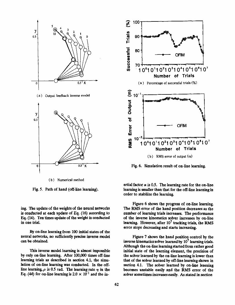
( a Output feedback inverse model

( b ) Numerical method

Fig. 5. Path of hand (off-line learning).

ing. The update of the weights of the neural networks is conducted at each update of Eq. (16) according to Eq. (14). Ten times update of the weight is conducted in one trial.

By on-line learning from 100 initial states of the neural networks, no sufficiently precise inverse model can be obtained.

This inverse model learning is almost impossible by only on-line learning. After 100,OOO times off-line learning trials as described in section 4.1, the simulation of on-line learning was conducted. In the off- line learning,p is 0.5 rad. The learning rate q in the Eq. (44) for on-line learning is 2.0 x 10'' and the in-

Y loo? u) - .!? 90 c - 2 80

OFlM u) u) Q) 0 5 70

1001 0'1 02i 031 041 051 oei o7 Number of Trials

( a ) Percentage of successful trials (%)

n

E - 10-l a a a 0

CI

CI

Y - OFlM L

2 2

z 1001 0'1 02i 031 041 051 0'1 0' u)

U Number of Trials

( b ) RMS error of output (m)

Fig. 6. Simulation result of on-line learning.

ertial factor a is 0.5. The learning rate for the on-line learning is smaller than that for the off-line learning in order to stabilize the learning.

Figure 6 shows the progress of on-line learning. The RMS error of the hand position decreases as the number of learning trials increases. The performance of the inverse kinematics solver increases by on-line learning. However, after lo7 tracking trials, the RMS error stops decreasing and starts increasing.

Figure 7 shows the hand position control by the inverse kinematics solver learned by lo' learning trials. Although the on-line learning started from rather good initial state of the learning element, the precision of the solver learned by the on-line learning is lower than that of the solver learned by off-line learning shown in section 4.1. The solver learned by on-line learning becomes unstable easily and the RMS error of the sober sometimes increases easily. As stated in section

62

Fig. 7. Path of hand (OFIM, on-line learning).

3.3, the possibility that a human forms the inverse kinematics solver by using only on-line learning is low.

43. Hybrid learning

The simulation of the hybrid learning that consists of both on-line and off-line is conducted.

The off-line learning is conducted when the arm moves from the end point of one tracking trial to the start point of the next tracking trial. When the change of the joint angle vector reaches

a trial of learning is conducted. 0.25 rad corresponds to 1.25 radh when the sampling period is 0.2 s. The learning rate 7 is 5.0 - and the inertial factor a is 0.5.

Figure 8 shows the progress of hybrid learning. It is understood that the RMS error decreases and the precision of the solver becomes higher as the number of trials increases. After lo7 tracking trials, the RMS error still keeps decreasing. The RMS error is 5.03 X

at lo8 tracking trials. The mean number of learning in one tracking trial is 16.3. Figure 9 shows the hand position control by the learned solver. As the off-line learning in section 4.1, the path of the hand is almost similar to that of the numerical method. It is understood that the solver learned by the hybrid learning has sufficient precision of the hand position control.

40

20

i 001 o i l 02i 031 041 051 o c i o7 Number of Trials

( a Percentage of successful trials (%)

OFIM

r 0

0 L lo-* r;

6 v) 1 0 ' ~

i 001 0'1 02i 031 04i 051 oe i 0' K

Number of Trials ( b ) RMS error of output (m)

Fig. 8. Simulation result of hybrid learning.

4.4. Solution for static inverse kinematics problems

The simulation solving static inverse kinematics problems by using the solver learned in section 4.3 is conducted. A trial for solving a static inverse kinematics problem is conducted as follows. First, a joint angle vector is generated by using uniform random number. Then, an inverse kinematics problem, which regards the hand position corresponding the joint angle vector as a desired position, is solved. The RMS error of the hand positions generated by the solver is measured for the evaluation of the solver. The 10,OOO desired hand positions were generated for the evaluation.

When a desired hand position is given, an initial joint angle vector M(0) is generated by using a uniform random generator. A desired hand trajectory is

63

5. Conclusions

Fig. 9. Path of hand (OFIM, hybrid learning).

defined by Eq. (43) and the tracking procedure of the trajectory is started as stated in section 2.5. If the norm of the error between the hand position and the desired position does not become smaller than the desired position, a new initial joint angle vector is generated and the tracking procedure is repeated.

The upper limit of the generation of the initial joint angle vector is 20 for one desired hand position. If no solution which satisfies the desired precision is obtained, the solver outputs the joint angle vector which generates the smallest hand position error in all tracking procedures as a solution of the inverse kinematics problem.

For comparison, the precision of the solver that uses the inverse kinematics model learned by DIM is estimated. In this chapter, DIM refers to the solver learned by DIM. A 4-layered neural network is used for DIM. The 1st layer of the networks has two neurons. The 2nd and 3rd layers have 15 neurons each. The 4th layer has three neurons. The learning by DIM is conducted from 10 initial states of the neural networks and the best learning result is selected for the evaluation. The RMS error of the OFIM is 6.39 X 10” m and the mean number of the initial value changes is 0.692 when the desired precision is 0.01 m. The RMS error is 5.48 x 10” m and the mean number of the initial value changes is 4.29 when the desired precision is 0.005 cm. The RMS error of DIM is 1.62 x lo-*. The precision of the output feedback inverse model is higher than that of DIM in this simulation.

In this paper, we proposed a new learning model which avoids the ill-posedness of the of the inverse kinematics problem and obtains an inverse kinematics solver of a human arm and corroborated its learning capability through numerical experiments.

DIM has another problem as a human learning model. The large-scale connection change is necessary before the inverse model is used for control after learning. When controlling the hand position, the input of the learning element is the desired change of the joint angles.

When learning, the input of the inverse model is the observed change of the joint angles. Though the desired change and the observed change should coin- cide, the difference of the characteristics of these two signals is large. The solution of this problem will be reported in the future.

Acknowledgement. The authors thank Dr. Mitsuo Kawato, the director of Department 3 of ATR Human Information Processing Research Laboratories, for providing papers and helpful comments. They also thank Dr. f i n Agah for his help in the translation of this paper.

REFERENCES

1. M. I. Jordan. Supervised learning and systems with excess degrees of freedom. COINS Technical Report, 88-27, 1-41 (1988).

2. M. Kuperstein. Neural model of adaptive hand- eye coordination for single postures. Nature, 239,

3. Y. Sakaguchi, M. Zama, T. Maeda, K. Nakano and T. Omori. Coordination System of Sensor System and Motor System I. Proc. 26-th Conference of society of Instrument and Control Engineering, pp.

4. D. E. Rumelhart, G. E. Hinton and R. J. Williams. Learning Internal Representation by Error Propa- gation. Parallel Distributed Processing, D. E. Rumelhart and J. L. MacClelland and the PDP Research Group (ed.), pp. 318-326, MIT Press (1986).

5. J. S. Albus. A new approach to manipulator control: the cerebellar model articulation controller (CMAC). Trans. ASME, J. Dynamic Systems, Measurement, and Control, 97, pp. 220-227 (1W5).

6. T. Kohonen. Formation of topographic maps and

pp. 1308-1311 (1988).

73-74 (1988).

64

columnar microstructures in nerve fields. Bi- ological Cybernetics, 35, pp. 63-72 (1979).

7. M. Kawato, K. Furukawa and R. Suzuki. A hierarchical neural-network model for control and learning of voluntary movement. Biological Cybernetics, 57, pp. 169-185 (1987).

8. T. Maeda and S. Tachi. Sensory integration of binocular visual space and kinesthetic space in visual reaching experiment. Trans. society of Instrument and Control Engineers, 29,2, pp. 201- 210 (1993).

9. H. V. Helmholtz. Handbuch der Physiologischen Optik, 2, 3rd ed. Hamburg und Leipzig, Voss (1911).

10. S. Shlaer. The relation between visual acuity and illumination. Journal of General Physiology, 21,

11. H. W. Leibowitz. The relation between the rate threshold for the perception of movement and luminance for various durations of exposure. Jour. Experimental Psychology, 49, pp. 829-830 (1955).

12. M. Kawato. An optimization and learning in neural networks for formation and control of coordinated movement. ATR TechnicalReport, TA-

13. A. P. Georgopoulos, J. F. Kalaska, R. Camhitiand J. T. Massey. On the relations between the direction of two-dimensional arm movements and cell discharge in primate motor cortex. Jour. Neuro- science, 2, pp. 1527-1537 (1982).

14. A. P. Georgopoulos, J. F. Kalaska, J. D. Crutcher, R. Caminiti and J. T. Massey. The representation of movement direction in the motor cortex: Single cell and population studies. Dynamical Aspects of NeocorticalFunction, G. M. Edelman, W. E. Gall, and W. M. Cowan (ed.), Neuroscience Research Foundation, pp. 501-524 (1984).

15. A. P. Georgopoulos, A. B. Schwartz and R. E. Kettner. Neuronal population coding of movement direction. Science, 233, pp. 1416-1419 (1986).

16. R. Caminiti, P. B. Johnson and A. Urbano. Mak- ing arm movements within different parts of space, dynamic aspects in the primate motor cortex. Jour. Neuroscience, 10, p. 2039 (1990).

pp. 165-188 (1937).

A-0086 (1990).

17. R. A. Anderson, G. K. Essick and R. M. Siegel. Encoding of spatial location by posterior parietal neurons. Science, 230, pp. 456-458 (1985).

18. M. Gentilucci, L. Fogassi, G. Luppino, M. Matelli, R. Camarda and G. Rizzolatti. Functional organi- zation of inferior area 6 in the macaque monkey. Experimental Brain Research, 71, pp. 475-490 (1988).

19. M. A. Arbib and B. Hoff. Trends in neural modeling for reach grasp. Insights into the Reach to Grasp Movement, K. M. B. Bennett, and U. Castiello ed., North-Holland, pp. 311-344 (1994).

20. K. Kurata. Role of cortical motor areas in voluntary movements. Brain and Nerve, 47, 12, pp.

21. E. V. Everts, Y. Shinoda and P. Wise. Neuro- physical Approaches to Higher Brain Functions. New York, Wiley (1984).

22. D. Bullock and S. Grossberg. Neural dynamics of planned arm movements: Emergent invariants and speed-accuracy properties during trajectory formation. Psychological Review, 95, pp. 49-90 (1988).

23. E. Oyama and S. Tachi. A study of human hand position control learning-output feedback inverse model. Proc. 1991 International Joint Conference on Neural Networks (IJCNN'91 Singapore), pp.

24. E. Oyama and S. Tachi. A learning method for solving inverse problems of static systems. Proc. 1993 International Joint Conference on Neural Networks (IJCNN'93 Nagoya), pp. 2843-2849 (1993).

25. D. E. Whitney. The mathematics of coordinated control of prosthetic arms and manipulators. Trans. ASME, J. Dynamic Systems, Measurement, and Control, 93, pp. 303-309 (1972).

26. J. S. Albus. Data storage in the cerebellar model articulation controller (CMAC). Trans. ASME, J. Dynamic Systems, Measurement, and Control, 97,

27. S. I. Colombano, M. Compton and M. Baulat. Goal Directed Model Inversion. Proc. of In- ternational Joint Conference on Neural Networks (IJCNN91 Singapore), pp. 2422-2427 (1991).

1135-1142 (1995).

1434-1443 (1991).

pp. 228-233 (1975).

65

Appendix 1. OtT-line Learning

APPENDIX

p(A6) = g(ABTAe)

From Eqs. (23) and (25),

Ae(Az, u) = J t (8)Az

is obtained. Assuming that rank(J(0)) is n, rank(1 - J+(ey(e)) is m - m. Let u* be an m x 1 vector n, components of which are appropriately selected and set 0. For a given u, u* that satisfies the following equation exists:

= ( I - J+(e)J(e))u* (48)

We can assume the following equationswith generality:

‘ I u* = (211, U 2 , . . . , u;-n, 0 , . . ., o y (49)

The correspondence between u’ and A@(&, u) is one- to-one. Hereafter,p(b) is designated as J+ . Because Eq. (28) contains a scaling term, the volume element dv can be identifiedwith du’. Therefore,

@ ( O , A z ) w E(AB*(Az,u))

The region of the integration U in the forementioned equation is the whole space of (m - n) x 1 vector u’ expressed as

00 00

h(u’)du’ = /, . . .LW h(u‘)du\ .... d u k - ,

(52)

Consider the distribution of A# to be spherical symmetry. In this case, the probability density function p ( U ) is the function of the square of the norm of A0 as

Let B be a rn x m matrix defined as

B = I - J + J

(53)

(54)

Since

J + ~ B = o (55)

is established,

is obtained. Becausep(M*) is an even function of each element of u’, and Bu* is an odd function of each element of u’, the integral of the product of p(be*) and Bu* is 0. Consequently,

S(6, A z ) $3 E(Ae*) = J’Az (57)

is obtained. The learning element calculates the mini- mum norm solution of Eq. (13).

Consider thatp(he) can be expressed as Eq. (32). Because P is a positive symmetric matrix, there exists an appropriate R that satisfies

P = R R ~ (58)

By the transformation of the variables as:

the same calculation as in the preceding equations can be used. Consequently,

@(8 ,Az ) w E(Ae*)

= RE(Ae’*)

= R J ’ ~ ( J’ J ’ ~ ) - dz

66

is obtained.

Appendix 2. Coordinate Transformation System Pay- ing Attention to Velocity and Acceleration

Coordinate transformation systems can be obtained by paying attention to the relationship between the joint angles velocity and the hand position velocity. Let 4(@, i ) be the output of neural networks, the output of which is the velocity command of the joint angles and @’(@, i) be the teaching signal of 4(@, i). We propose the learning method of We, i) as follows:

As the coordinate transformation system calculating the velocity command of the joint angles, the coordinate transformation system 4(@, d, 2) calculating the acceleration command of the joint angles can be obtained by the teaching signal defined as

e* that satisfies Eq. (20) can be expressed as

According to the learning shown in Eq. (M),

a q e , ~ ) = e (61)

As the coordinate transformation system based on the change of the joint angle vector described in section

q e , b, 2) M ~ ( e j = J * ( e ) ( g - [-e]e) aJ(e> ae

(66) 3.1,

is obtained. @(@, i, ;;> is the inverse model of the sys- e = @(e,i) tem described in Eq. (20) that can transform the accel-

eration of the hand to the acceleration of the joint E@*) = q e ) i (62) angles.

is obtained. @(@, i ) is the inverse model of the system described in Eq. (19). By inputting the desired hand velocity, including the position error feedback

By inputting the desired hand acceleration including the position and velocity error feedback

$& = $ d + K g ( & d - k) + K ( Z d - Z) (67)

to @(O, i , Z ) , the acceleration command of the joint angles that makes the hand tracking the desired hand position can be calculated. KO is an appropriate velocity feedback gain.

X& = X d + K ( Z d - Z) (63)

to @(@, i), the velocity command of the joint angles that makes the hand tracking the desired hand position can be calculated.

AUTHORS

Eimci Oyama received his B.E. degree in 1985 and his M.E. degree in 1987 in Aeronautics from the University of Tokyo. He joined MEL (Mechanical Engineering Laboratory), AIST, MITI, Japan, in 1987 and was a Research Associate in the Man-Machine System Division, Robotics Department from 1987 to 1994. He has been a Senior Researcher at Bio-Robotics Division since 1994. His research interests include human motion control system, neuroscience, computer vision, nonlinear optimization, man-machine interface and teleexistence. He is a member of IEICE (the Institute of Electronics, Information and Communication Engineers); RSJ (Robotics Society Japan); SICE (the Society of Instrument and Control Engineers); and JSME (the Japan Society of Mechanical Engineers).

67

AUTHORS (continued, from left to right)

Tam Ma& received his B.E. degree in 1987 and Dr. of Eng. degree in 1994 in Mathematical Engineering and Information Physics from the University of Tokyo. He joined Mechanical Engineering Laboratory, AIST in 1987 and was a Research hmciate in the Man-Machine System Division, Robotics Department from 1987 to 1992. He was a Research Associate at RCAST (Research Center of Advanced Science and Technology), the University of Tokyo from 1992 to 1994. He has been a Research Associate at the University of Tokyo since 1994. His research interests include human perception system, human motion control system, neuroscience, neural computation, man-machine interface, and teleexistence. He is a member of IEICE RSJ; SICE; JSME; JNNS (Japanese Neural Network Society).

Susumu Tacbi received his B.E. degree in 1968 and his Dr. of Eng. degree in 1973 in Mathematical Engineering and Information Physics from the University of Tokyo. He was a Research Associate at the University of Tokyo, a Researcher at Mechanical Engineering Laboratory, AIST, a Senior Researcher, Director of Man-Machine System Divi- sion, Director of Bio-Robotics Division and an Assistant Professor at the University of Tokyo. He has been a Professor at the University of Tokyo since 1992. He was a Visiting Researcher at MIT from 1979 to 1980. His research interests include signal processing using spectrum analysis, guide dog robot, virtual reality and teleexistence. He is a member of RSJ; SICE; JSME; IEEE; and IMECO. He was the chair of IMECO TC 17 (Robotics) and is an SICE Fellow.

68

Documents

A human system learning model for solving the inverse kinematics problem by direct inverse modeling