Embed Size (px)
Citation preview
September, 2011
IRI-TR-11-01
Smooth Inverse KinematicsAlgorithms for Serial Redundant Robots
Master Thesis
Adria Colome
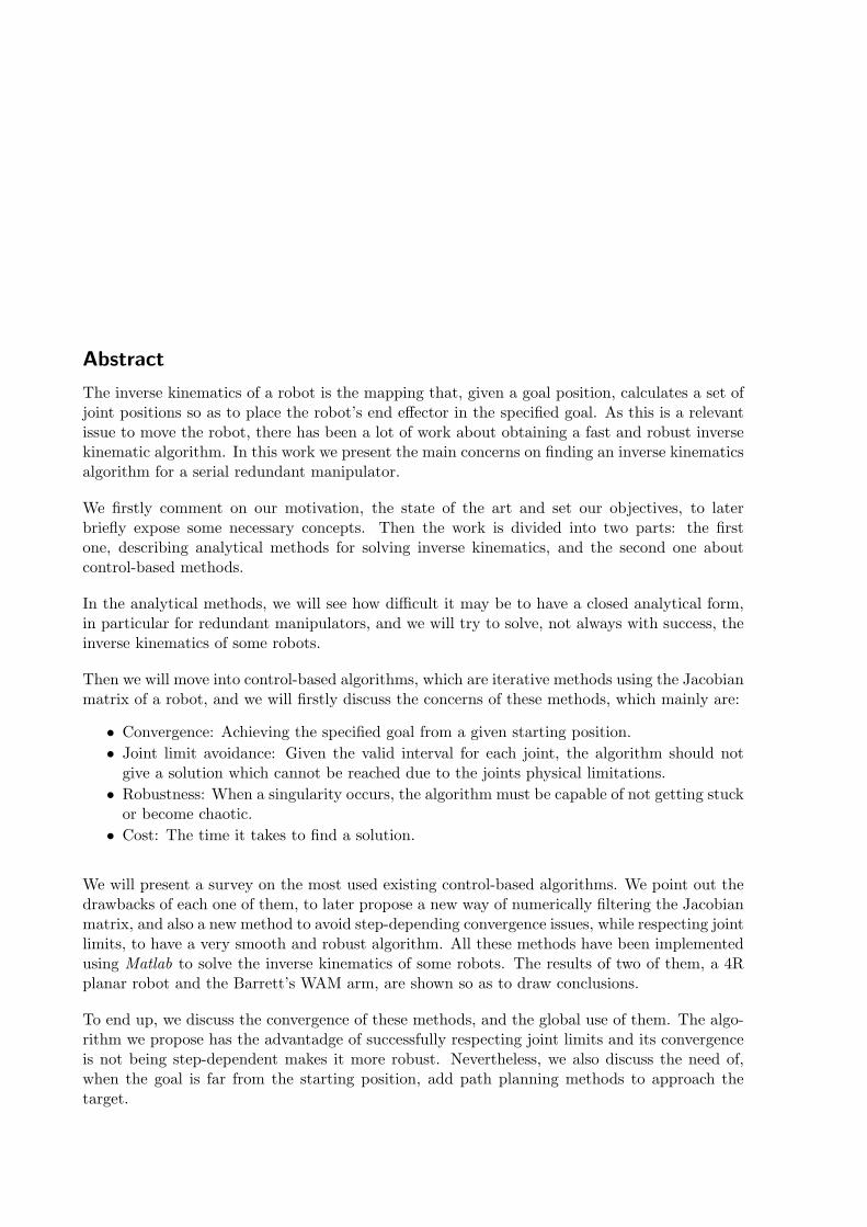
Abstract
The inverse kinematics of a robot is the mapping that, given a goal position, calculates a set ofjoint positions so as to place the robot’s end effector in the specified goal. As this is a relevantissue to move the robot, there has been a lot of work about obtaining a fast and robust inversekinematic algorithm. In this work we present the main concerns on finding an inverse kinematicsalgorithm for a serial redundant manipulator.
We firstly comment on our motivation, the state of the art and set our objectives, to laterbriefly expose some necessary concepts. Then the work is divided into two parts: the firstone, describing analytical methods for solving inverse kinematics, and the second one aboutcontrol-based methods.
In the analytical methods, we will see how difficult it may be to have a closed analytical form,in particular for redundant manipulators, and we will try to solve, not always with success, theinverse kinematics of some robots.
Then we will move into control-based algorithms, which are iterative methods using the Jacobianmatrix of a robot, and we will firstly discuss the concerns of these methods, which mainly are:
• Convergence: Achieving the specified goal from a given starting position.
• Joint limit avoidance: Given the valid interval for each joint, the algorithm should notgive a solution which cannot be reached due to the joints physical limitations.
• Robustness: When a singularity occurs, the algorithm must be capable of not getting stuckor become chaotic.
• Cost: The time it takes to find a solution.
We will present a survey on the most used existing control-based algorithms. We point out thedrawbacks of each one of them, to later propose a new way of numerically filtering the Jacobianmatrix, and also a new method to avoid step-depending convergence issues, while respecting jointlimits, to have a very smooth and robust algorithm. All these methods have been implementedusing Matlab to solve the inverse kinematics of some robots. The results of two of them, a 4Rplanar robot and the Barrett’s WAM arm, are shown so as to draw conclusions.
To end up, we discuss the convergence of these methods, and the global use of them. The algo-rithm we propose has the advantadge of successfully respecting joint limits and its convergenceis not being step-dependent makes it more robust. Nevertheless, we also discuss the need of,when the goal is far from the starting position, add path planning methods to approach thetarget.

0
Institut de Robotica i Informatica Industrial (IRI)Consejo Superior de Investigaciones Cientıficas (CSIC)
Universitat Politecnica de Catalunya (UPC)Llorens i Artigas 4-6, 08028, Barcelona, Spain
Tel (fax): +34 93 401 5750 (5751)
http://www.iri.upc.edu
Corresponding author:
Adria Colometel: +34 93 401 5791
http://www.iri.upc.edu/staff/acolome
Copyright IRI, 2011
CONTENTS 1
Contents
1 Preliminaries 31.1 Motivation . . . . . . . . . . . . . . . . . . . . . . . . . . . . . . . . . . . . . . . 31.2 State of the art . . . . . . . . . . . . . . . . . . . . . . . . . . . . . . . . . . . . . 31.3 Objectives . . . . . . . . . . . . . . . . . . . . . . . . . . . . . . . . . . . . . . . . 3
2 Introduction 52.1 Forward and inverse kinematics of a serial manipulator . . . . . . . . . . . . . . . 52.2 Denavit-Hartenberg parameters . . . . . . . . . . . . . . . . . . . . . . . . . . . . 5
3 Robot positioning 73.1 Robot differential kinematics . . . . . . . . . . . . . . . . . . . . . . . . . . . . . 73.2 Desired position and error representation . . . . . . . . . . . . . . . . . . . . . . 73.3 Criteria for optimizing redundant degrees of freedom . . . . . . . . . . . . . . . . 8
3.3.1 Manipulability . . . . . . . . . . . . . . . . . . . . . . . . . . . . . . . . . 83.3.2 Joint limit avoidance . . . . . . . . . . . . . . . . . . . . . . . . . . . . . . 93.3.3 Other Criteria . . . . . . . . . . . . . . . . . . . . . . . . . . . . . . . . . 9
4 Analytical methods for inverse kinematics 114.1 General procedure . . . . . . . . . . . . . . . . . . . . . . . . . . . . . . . . . . . 11
4.1.1 3R manipulator . . . . . . . . . . . . . . . . . . . . . . . . . . . . . . . . . 114.2 Spherical Wrists . . . . . . . . . . . . . . . . . . . . . . . . . . . . . . . . . . . . 124.3 Redundant degrees of freedom optimization . . . . . . . . . . . . . . . . . . . . . 134.4 Examples . . . . . . . . . . . . . . . . . . . . . . . . . . . . . . . . . . . . . . . . 13
4.4.1 3R redundant planar manipulator . . . . . . . . . . . . . . . . . . . . . . 134.4.2 Laparoscopic robot . . . . . . . . . . . . . . . . . . . . . . . . . . . . . . . 144.4.3 Barrett’s WAM arm . . . . . . . . . . . . . . . . . . . . . . . . . . . . . . 17
5 Time-discrete control-based methods 215.1 General schemes . . . . . . . . . . . . . . . . . . . . . . . . . . . . . . . . . . . . 215.2 About the convergence of control-based methods . . . . . . . . . . . . . . . . . . 215.3 Methods from literature . . . . . . . . . . . . . . . . . . . . . . . . . . . . . . . . 22
5.3.1 Jacobian pseudoinverse . . . . . . . . . . . . . . . . . . . . . . . . . . . . 235.3.2 Jacobian transpose . . . . . . . . . . . . . . . . . . . . . . . . . . . . . . . 265.3.3 Jacobian damping and filtering . . . . . . . . . . . . . . . . . . . . . . . . 275.3.4 Selectively damped least squares. . . . . . . . . . . . . . . . . . . . . . . . 295.3.5 Gradient projection . . . . . . . . . . . . . . . . . . . . . . . . . . . . . . 335.3.6 Task priority . . . . . . . . . . . . . . . . . . . . . . . . . . . . . . . . . . 335.3.7 Jacobian Weighting Methods . . . . . . . . . . . . . . . . . . . . . . . . . 365.3.8 Joint Clamping . . . . . . . . . . . . . . . . . . . . . . . . . . . . . . . . . 375.3.9 Continuous Clamping . . . . . . . . . . . . . . . . . . . . . . . . . . . . . 41
5.4 Proposed methods . . . . . . . . . . . . . . . . . . . . . . . . . . . . . . . . . . . 445.4.1 Smooth eigenvalue filtering. . . . . . . . . . . . . . . . . . . . . . . . . . . 445.4.2 Continuous Clamping combined with Selective Damping . . . . . . . . . . 48
6 Experimental Results 566.1 4R planar robot . . . . . . . . . . . . . . . . . . . . . . . . . . . . . . . . . . . . . 566.2 Barret’s WAM arm . . . . . . . . . . . . . . . . . . . . . . . . . . . . . . . . . . . 60
7 Conclusions and Future Work 68

2 CONTENTS
Section 1 Preliminaries 3
1 Preliminaries
1.1 Motivation
Year after year, more complex serial robots are designed and built. Many of them with multiplelimbs (arms / fingers) and redundant, in the sense that they are overarticulated. This overartic-ulation gives more flexibility, and now robots can not only reach a position, but also reach it inseveral configurations, and so secondary goals can be achieved.
Nevertheless, this complexity on the robots has a drawback, which is the computation of theirkinematics. The kinematics map of a serial robot is not a bijection. In particular, the kinematicsof a serial robots is a surjective function with its reachable workspace (i.e.: a mapping f : X → Yso that ∀ y ∈ Y , there exists one or more x ∈ X so that f(x) = y), in the sense that two differentjoint states can give the same position of the end effector of a robot.
The initial aim of this project has been to find an efficient, continuous solution for the inversekinematics of the Barrett’s WAM arm, a robot available in the Institut de Robotica i InformaticaIndustrial (IRI), whose of-the-shelf inverse kinematics series algorithm is not optimum. Thisaim has been focused on analysing its inverse kinematics by analytical methods, but also withcontrol-based methods, to compare their solutions.
1.2 State of the art
Inverse kinematics algorithms have been an issue to focus on since the first robots were built.To do so, the most popular methods have been the analytical (and so exact) ones. Nevertheless,an exact solution does not always exist, and when one has to look for an alternative solution,the most popular methods are the control-based ones, although there also exist methods basedon learning, neural networks [22], interval methods [16], or based on distances [15].
On control-based methods, the first approaches were developed in the 60s-70s, when Whitney[23] used the pseudoinverse of a matrix to solve the problem. Although other methods such asthe Jacobian transpose [24], which can be faster, were used as well. Lately in the 1980s, withthe rising computation capability of computers, Baillieul [1] presented an extended Jacobian,which was computationally more complex, with second-order derivatives. Also in the 80s, themanipulability index was defined by Yoshikawa [25], a term to optimize when having a redundantrobot.
Since then, many ways of improving the performance of these algorithms have been proposed.Siciliano and Slotine presented in 1991 a hierarchical way to priorisize different tasks [19], andparallelly, the damping of the Jacobian, a way of avoiding the discontinuity of the pseudoinverseoperator when the Jacobian matrix of a robot looses rank, was presented and analised [6] withits variants [5]. In the 90s is when it began to be also very common to weight the Jacobianmatrix of a manipulator in order to prioritisize joints or tasks over others [3], or even blockcertain movements with these weighting matrices.
But it has not been until the 2000s that the continuity of these methods started having arelevant paper in the design of algorithms. In [17], Raunhart and Boulic try to continuouslyblock the motion of a joint, and finally in [13], Mansard, Remazeilles and Chaumette define anew pseudoinverse operator to be smooth with respect to the joint/task blocking, to be usedlater in [12], combining this continuous pseudoinverse operator with a task priority scheme.
1.3 Objectives
As commented on the motivation, our objective is to find an analytical solution for the inversekinematics of redundant robots, and regarding control-based methods, to obtain the smoothestalgorithm as possible, leading to a robust iterative method.

4 Master Thesis
To do so, our intention is, after considering the analytical ways of solving the problem, todescribe the most popular existing control-based methods, trying to point out their limitationsand difficulties, in a survey-like way, to then try to take the best of each of them and find arobust solution, checking its behaviour and comparing it to the analytical one.
Section 2 Introduction 5
2 Introduction
Controlling the position of a robot is not as trivial as one could think. Serial robots are com-posed of concatenated joints, forming an open chain structure. With this structure, the inversekinematic problem, that is, relating the position and/or orientation of the end effector of themanipulator with the position of each joint, might not have a closed analytical solution. Nothaving such an analytical solution can force the user to search for alternative solutions to thekinematics of the robot. And even when a closed analytical form exists, its equations may havemultiple solutions.
Ever since the first industrial robots appeared, there has been a big concern about computingkinematics in a simple, reliable and fast way in order to optimize the robot performance. Inthis work, we analyse the state of the art on the computation of inverse kinematics, pointingout the weaknesses of all the methodologies considered, and aiming to take the best of themto obtain an inverse kinematics algorithm which is robust and reliable, with special attentionto redundant robots (those with more degrees of freedom than supposely needed to perform aspecified task).
2.1 Forward and inverse kinematics of a serial manipulator
Let us consider a serial robot with m joints, and let W ⊆ Rn be its workspace (reachablepositions) in a space of dimension n (n=2 for planar position, 3 for planar position+orientationor spatial position, 6 for spatial position+orientation, etc.). Then we define:
• The Forward Kinematics as the function that maps a joint position of the set Q offeasible joint positions into a cartesian position in the workspace W
f : Q ⊆ Rm → W ⊆ Rn
q 7→ x
The forward kinematics function is easily obtained for serial manipulators with theDenavit-Hartenberg coefficients (see section 4.4.3). By construction, W = ImQ(f)
• The Inverse Kinematics is the inverse mapping of the Forward kinematics, i.e.: thefunction that maps a position in the workspace to a joint position:
h : W ⊆ Rn → Q ⊆ Rm
x 7→ q
Note that h can have multiple solutions for a single x, or even infinite solutions in case m >n or in a degenerate position. Finding a closed expression for h can be very complicated oreven impossible, and when handling with trigonometric functions, more than one solutionmay arise.
2.2 Denavit-Hartenberg parameters
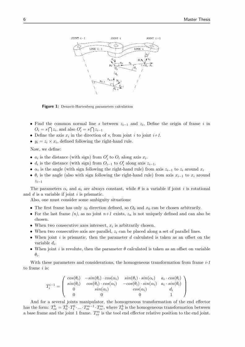
When considering a serial open-chain manipulator, a systematic way of expressing its forwardkinematics is using the Denavit-Hartenberg convention. This consists in defining the relativeposition and orientation of two consecutive links, and determining a transformation matrixbetween them, by performing the following operations (see Figure 1):
First, consider axis zi−1 as the axis of the joint between link i-1 and link i. To define thehomogeneous transformation between frames i-1 and i :
• Set axis zi as the axis of rotation or movement of joint i+1.
6 Master Thesis
Figure 1: Denavit-Hartenberg parameters calculation
• Find the common normal line s between zi−1 and zi, Define the origin of frame i inOi = s
⋂
zi, and also O′i = s
⋂
zi−1
• Define the axis xi in the direction of s, from joint i to joint i+1.
• yi = zi × xi, defined following the right-hand rule.
Now, we define:
• ai is the distance (with sign) from O′i to Oi along axis xi.
• di is the distance (with sign) from Oi−1 to O′i along axis zi−1.
• αi is the angle (with sign following the right-hand rule) from axis zi−1 to zi around xi• θi is the angle (also with sign following the right-hand rule) from axis xi−1 to xi around
zi−1
The parameters αi and ai are always constant, while θ is a variable if joint i is rotationaland d is a variable if joint i is prismatic.
Also, one must consider some ambiguity situations:
• The first frame has only z0 direction defined, so O0 and x0 can be chosen arbitrarily.
• For the last frame (n), as no joint n+1 exists, zn is not uniquely defined and can also bechosen.
• When two consecutive axes intersect, xi is arbitrarily chosen.
• When two consecutive axis are parallel, zi can be placed along a set of parallel lines.
• When joint i is prismatic, then the parameter d calculated is taken as an offset on thevariable di.
• When joint i is revolute, then the parameter θ calculated is taken as an offset on variableθi.
With these parameters and considerations, the homogeneous transformation from frame i-1to frame i is:
T i−1i =
cos(θi) −sin(θi) · cos(αi) sin(θi) · sin(αi) ai · cos(θi)sin(θi) cos(θi) · cos(αi) −cos(θi) · sin(αi) ai · sin(θi)
0 sin(αi) cos(αi) di0 0 0 1
And for a several joints manipulator, the homogeneous transformation of the end effectorhas the form: T b
ee = T b0 ·T 0
1 · ... ·Tm−1m ·Tm
ee , where Tb0 is the homogeneous transformation between
a base frame and the joint 1 frame. Tmee is the tool end effector relative position to the end joint.
Section 3 Robot positioning 7
3 Robot positioning
Positioning a robot in its workspace requires calculating its inverse kinematics. In this section,we introduce the basic concepts for understanding the following sections in a very practical andfocused way.
3.1 Robot differential kinematics
There is much literature about differential kinematics, in terms of joints and position velocityand accelerations, etc. But here we will focus on what will be used later. For further reading,we recommend [20], chapter 3.
Given a serial manipulator, one might want not only to know its direct and inverse kinematics,but also its differential kinematics. In this sense, a fundamental tool is the Geometric Jacobianof a manipulator at a given joint state θ, which gives the differential position/orientation first-order variation of the end effector of a manipulator, depending on the differential first-ordervariation of each joint, i.e.:
x = J · θ, (1)
where θ is the time-derivative of the joints, and x is the generalized coordinate vector in thecartesian space:
x =
(
xeφe
)
,
φe being a set of Euler angles describing the orientation of the end effector.
Column i of the Jacobian J represents the effect of ith joint on the generalised coordinatesof the end effector.
To compute this Jacobian in a m-link robot, this formula can be applied (see [20], pp111-113):
J =
[
JP1 ... JPm
JO1 ... JOm
]
,
where:
[
JPi
JOi
]
=
[
zi−1
0
]
if the joint is prismatic, and
[
JPi
JOi
]
=
[
zi−1 × (Pe − Pi−1)zi−1
]
if the joint is revolute,
where Pe is the position of the end effector of the robot and Pi−1 is the position vector ofthe origin of frame i-1, both expressed in the base frame.
3.2 Desired position and error representation
Depending on the type of robot and the task to be performed, the state vector may vary from a2 -dimentional position (x, y) to a generalized 6-dimensional position and orientation vector. Inany case, a planar position is a projection of the generalised coordinate vector.
8 Master Thesis
Now, to express the orientation error, given a desired position and/or orientation, if we takethe non-minimal representation of the actual orientation as the rotation matrix
Re(θ) =(
ne(θ) se(θ) ae(θ))
,
and equally with the desired orientation:
Rd =(
nd sd ad)
,
then the orientation error can be represented as (see [20], pp 137-140):
eo =1
2(ne(θ)× nd + se(θ)× sd + ae(θ)× ad), (2)
while the position error is:
eP = xd − xe(θ) (3)
This error representation will be useful to perform control-based methods for inverse kine-matics.
3.3 Criteria for optimizing redundant degrees of freedom
When dealing with redundant manipulators, as the robot has more degrees of freedom thannecessary to perform a certain task, the remaining degrees of freedom give a set of feasiblesolutions of the inverse kinematics. Among these solutions, it is recommended to choose the onesatisfying a certain criterion: A secondary goal, an additional restriction, etc. For almost everypossible task, a potential function can be created; if H : Rm → R is a cost function, a gradientof the form ~h = −▽H can be used. Now we will describe some criteria that are often used.
3.3.1 Manipulability
The manipulability of a robot in a given configuration θ was first introduced by Yoshikawa [25],and it is defined as: w(q) =
√
|det(J(θ) · J(θ)T )|.With a singular value decomposition, and using det(AB) = det(A)det(B), it can be easily
proven that w(q) =∏
σi, the product of the eigenvectors of J, and now we will see someproperties of interest of this term:
Consider the set of joint velocities of constant unit norm
θT · θ = 1. (4)
Assuming full-rank matrix J, we can set a minimum norm solution of the inverse kinematicsfrom (1)
θ = J† · x, (5)
where J† = JT · (J ·JT )−1 is the Moore-Penrose pseudoinverse matrix of J. This set of velocitiesmaps, through equations (4) and (5), to a corresponding set of cartesian space velocities (usingpseudoinverse properties and assuming full-row rank of J):
vTe · (J†T · J†) · ve = vTe · (J · JT )−1 · ve = 1,
which is the equation of the points on the surface of an ellipsoid in the end effector velocity space.The eigenvectors of matrix J · JT give the principal axes of the ellipsoid, and its eigenvaluesgive the width of the ellispoid along the corresponding eigenvectors. This ellipsoid gives an idea
Section 3 Robot positioning 9
−0.6 −0.4 −0.2 0 0.2 0.4 0.6 0.8 10
0.1
0.2
0.3
0.4
0.5
0.6
0.7
0.8
0.9
1Manipulability ellipsoids for a 4R planar robot
X position
Y p
ositi
on
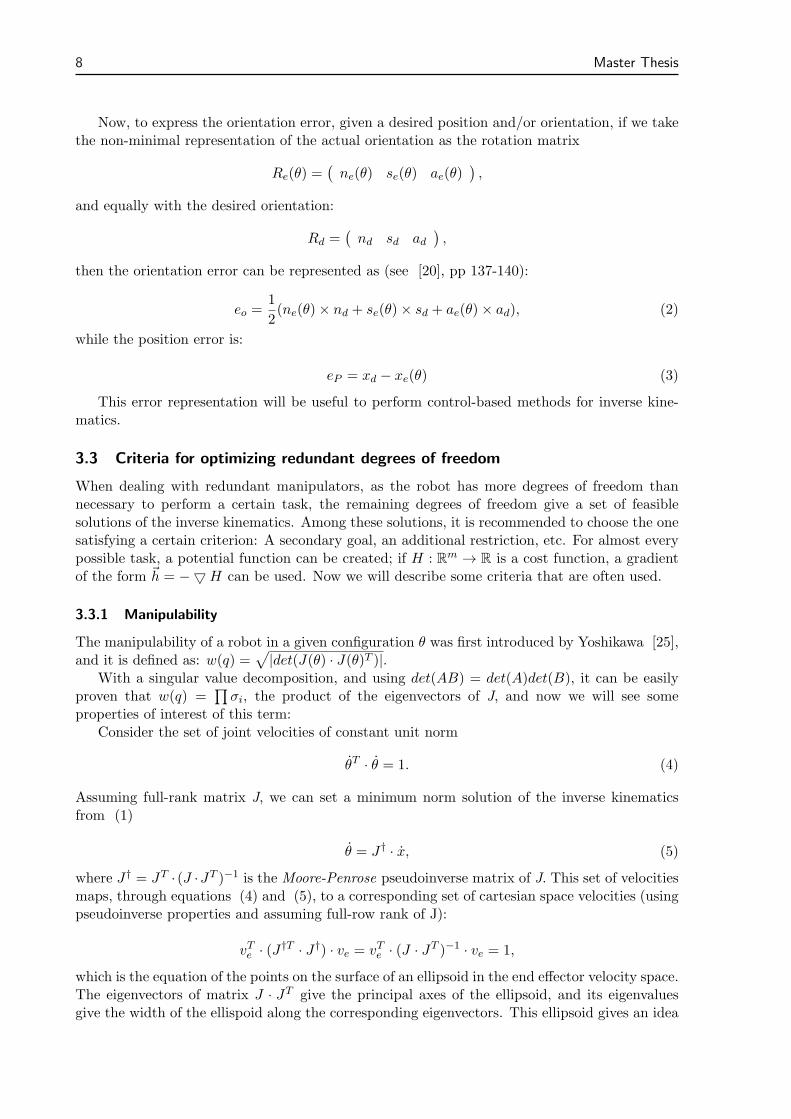
Figure 2: Manipulability ellipsoids (scaled to fit in the image). Here it can be seen that,when approaching a singularity, the task Jacobian looses rank, and the manipulabilityellipsoid’s area becomes zero.
of the behaviour of the end effector in the neighbourhood of the actual state, and its volume isproportional to w(θ) =
√
|det(J(θ) · J(θ)T )|. What has to be considered with manipulability isthe fact that if one eigenvalue of J · JT is zero, so is the manipulability index, meaning that ifJ is rank-deficient, the robot is in a singular position. Also, the higher the manipulability, theless excentricity the manipulability ellipsoid will have, the farther the robot from a singularitywill be, and the more isotropic the movement capabilities of the robot are in that position.
In Figure 2 we can see how the manipulability ellipsoid varies with position for a 4R planarrobot, and has 0 area at a singularity.
The convenience of using this criterion has been longly discussed, and a similar term as a ma-nipulability polytope (see [10]) may reflect the robot’s behaviour better, but it is computationallyslower.
3.3.2 Joint limit avoidance
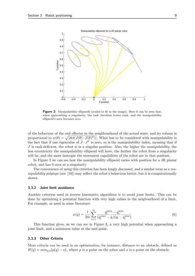
Another criterion used in inverse kinematics algorithms is to avoid joint limits. This can bedone by optimizing a potential function with very high values in the neigbourhood of a limit.For example, as used in some literature:
w(q) =1
2m
m∑
i=1
qmaxi − qmin
i
(qmaxi − qi)(qi − qmin
i )(6)
This function gives, as we can see in Figure 3, a very high potential when approaching ajoint limit, and a minimum value at the mid point.
3.3.3 Other Criteria
More criteria can be used in an optimization, for instance, distance to an obstacle, defined asH(q) = minp,o‖p(q)− o‖, where p is a point on the robot and o is a point on the obstacle.
10 Master Thesis
−1 −0.8 −0.6 −0.4 −0.2 0 0.2 0.4 0.6 0.8 10
1
2
3
4
5
6
7
8
9
10
w(q
)
q
Joint limit avoidance potential function
Figure 3: The potential function rises when approaching joint limits.
Another example would be, for a mobile robot, to keep the vertical projection of its center ofmass inside a region, which could be the polygon defined by the feet in contact with the ground(legged robot), or its wheels (wheeled robot) , to mantain its equilibrium.
Section 4 Analytical methods for inverse kinematics 11
4 Analytical methods for inverse kinematics
When trying to compute inverse kinematics of a manipulator, a recommended first approach isto compute an analytical solution, as it will be an exact solution, and usually faster to computethan any other.
4.1 General procedure
As for a serial robot direct kinematics equations are often easy to obtain (in complex serialrobots, the use of the D-H parameters might be useful, although other methodologies exist), away to start is trying to find the inverse function of the direct kinematics. As many trigonomet-ric functions may appear when dealing with rotational joints, this inversion can require somealgebraic skills, as it will usually be non-trivial, or even impossible. Moreover, multiple solutionsof trigonometric functions must be considered. This derives in multiple solutions of the inversekinematics, called assembly modes.
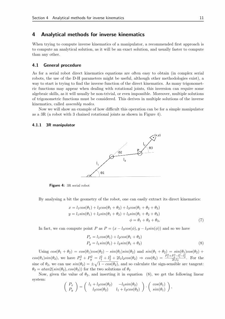
Now we will show an example of how difficult this operation can be for a simple manipulatoras a 3R (a robot with 3 chained rotational joints as shown in Figure 4).
4.1.1 3R manipulator
Figure 4: 3R serial robot
By analysing a bit the geometry of the robot, one can easily extract its direct kinematics:
x = l1cos(θ1) + l2cos(θ1 + θ2) + l3cos(θ1 + θ2 + θ3)
y = l1sin(θ1) + l2sin(θ1 + θ2) + l3sin(θ1 + θ2 + θ3)
φ = θ1 + θ2 + θ3, (7)
In fact, we can compute point P as P = (x− l3cos(φ), y − l3sin(φ)) and so we have
Px = l1cos(θ1) + l2cos(θ1 + θ2)
Py = l1sin(θ1) + l2sin(θ1 + θ2) (8)
Using cos(θ1 + θ2) = cos(θ1)cos(θ2) − sin(θ1)sin(θ2) and sin(θ1 + θ2) = sin(θ1)cos(θ2) +
cos(θ1)sin(θ2), we have P 2x + P 2
y = l21 + l22 + 2l1l2cos(θ2) ⇒ cos(θ2) =P 2x+P 2
y−l21−l2
2
2l1l2. For the
sine of θ2, we can use sin(θ2) = ±√
1− cos(θ2), and so calculate the sign-sensible arc tangent:θ2 = atan2(sin(θ2), cos(θ2)) for the two solutions of θ2
Now, given the value of θ2, and inserting it in equation (8), we get the following linearsystem:
(
Px
Py
)
=
(
l1 + l2cos(θ2) −l2sin(θ2)l2cos(θ2) l1 + l2cos(θ2)
)
·(
cos(θ1)sin(θ1)
)
,
12 Master Thesis
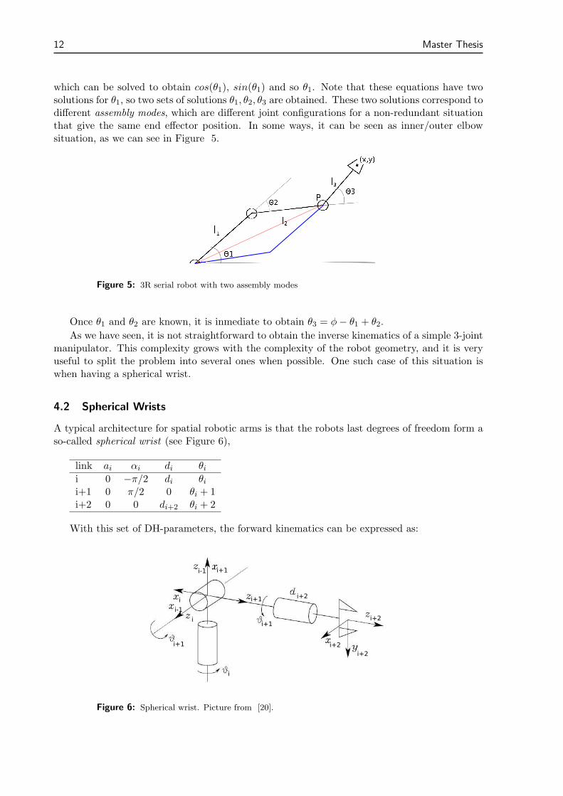
which can be solved to obtain cos(θ1), sin(θ1) and so θ1. Note that these equations have twosolutions for θ1, so two sets of solutions θ1, θ2, θ3 are obtained. These two solutions correspond todifferent assembly modes, which are different joint configurations for a non-redundant situationthat give the same end effector position. In some ways, it can be seen as inner/outer elbowsituation, as we can see in Figure 5.
Figure 5: 3R serial robot with two assembly modes
Once θ1 and θ2 are known, it is inmediate to obtain θ3 = φ− θ1 + θ2.
As we have seen, it is not straightforward to obtain the inverse kinematics of a simple 3-jointmanipulator. This complexity grows with the complexity of the robot geometry, and it is veryuseful to split the problem into several ones when possible. One such case of this situation iswhen having a spherical wrist.
4.2 Spherical Wrists
A typical architecture for spatial robotic arms is that the robots last degrees of freedom form aso-called spherical wrist (see Figure 6),
link ai αi di θii 0 −π/2 di θii+1 0 π/2 0 θi + 1i+2 0 0 di+2 θi + 2
With this set of DH-parameters, the forward kinematics can be expressed as:
i
i+2
i+2
i+2
i+1
i+1
i
i+1
i-1
i-1
i
i+2i+1
Figure 6: Spherical wrist. Picture from [20].
Section 4 Analytical methods for inverse kinematics 13
Pee
Origin
Joint 1 sphere
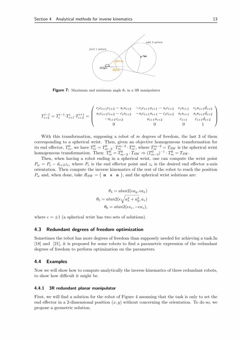
Joint 3 sphere
Figure 7: Maximum and minimum angle θ1 in a 3R manipulator
T i−1i+2 = T i−1
i ·T ii+1·T i+1
i+2 =
cici+1ci+2 − sisi+2 −cici+1si+1 − sici+2 cisi+1 cisi+1di+2
sici+1ci+2 − cisi+2 −sici+1si+1 − cici+2 sisi+1 sisi+1di+2
−si+1ci+2 si+1si+2 ci+1 ci+1di+2
0 0 0 1
With this transformation, supposing a robot of m degrees of freedom, the last 3 of themcorresponding to a spherical wrist. Then, given an objective homogeneous transformation forits end effector, T 0
ee, we have T 0ee = T 0
m−3 · Tm−3m · Tm
ee , where Tm−3m = TSW is the spherical wrist
homogeneous transformation. Then: T 0m = T 0
m−3 · TSW ⇒ (T 0m−3)
−1 · T 0m = TSW .
Then, when having a robot ending in a spherical wrist, one can compute the wrist pointPw = Pe − di+2ze, where Pe is the end effector point and ze is the desired end effector z-axisorientation. Then compute the inverse kinematics of the rest of the robot to reach the positionPw and, when done, take RSW =
(
n s a)
, and the spherical wrist solutions are:
θ4 = atan2(ǫay, ǫax)
θ5 = atan2(ǫ√
a2x + a2y, az)
θ6 = atan2(ǫsz,−ǫnz),
where ǫ = ±1 (a spherical wrist has two sets of solutions).
4.3 Redundant degrees of freedom optimization
Sometimes the robot has more degrees of freedom than supposely needed for achieving a task.In[18] and [21], it is proposed for some robots to find a parametric expression of the redundantdegrees of freedom to perform optimization on the parameters.
4.4 Examples
Now we will show how to compute analytically the inverse kinematics of three redundant robots,to show how difficult it might be.
4.4.1 3R redundant planar manipulator
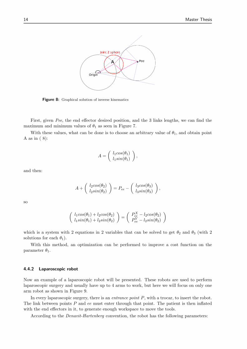
First, we will find a solution for the robot of Figure 4 assuming that the task is only to set theend effector in a 2-dimensional position (x, y) without concerning the orientation. To do so, wepropose a geometric solution.
14 Master Thesis
Pee
Origin
Figure 8: Graphical solution of inverse kinematics
First, given Pee, the end effector desired position, and the 3 links lengths, we can find themaximum and minimum values of θ1 as seen in Figure 7.
With these values, what can be done is to choose an arbitrary value of θ1, and obtain pointA as in ( 8):
A =
(
l1cos(θ1)l1sin(θ1)
)
,
and then:
A+
(
l2cos(θ2)l2sin(θ2)
)
= Pee −(
l3cos(θ3)l3sin(θ3)
)
,
so
(
l1cos(θ1) + l2cos(θ2)l1sin(θ1) + l2sin(θ2)
)
=
(
PXee − l2cos(θ2)
P Yee − l2sin(θ2)
)
which is a system with 2 equations in 2 variables that can be solved to get θ2 and θ3 (with 2solutions for each θ1).
With this method, an optimization can be performed to improve a cost function on theparameter θ1.
4.4.2 Laparoscopic robot
Now an example of a laparoscopic robot will be presented. These robots are used to performlaparoscopic surgery and usually have up to 4 arms to work, but here we will focus on only onearm robot as shown in Figure 9.
In every laparoscopic surgery, there is an entrance point P , with a trocar, to insert the robot.The link between points P and ee must enter through that point. The patient is then inflatedwith the end effectors in it, to generate enough workspace to move the tools.
According to the Denavit-Hartenberg convention, the robot has the following parameters:
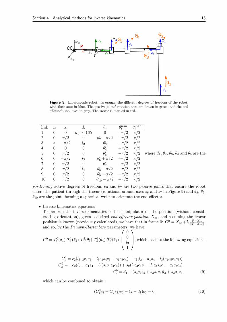
Section 4 Analytical methods for inverse kinematics 15
z0
1
2
3
4
5
6
7
z
z
z
z
z
z
z
P
C
ΘΘ
Θ
2
3
4
1d
Θ5z
z
8
ee
Figure 9: Laparoscopic robot. In orange, the different degrees of freedom of the robot,with their axes in blue. The passive joints’ rotation axes are drawn in green, and the endeffector’s tool axes in grey. The trocar is marked in red.
link ai αi di θi θmini θmax
i
1 0 0 d1+0.165 0 −π/2 π/22 0 π/2 0 θ′2 − π/2 −π/2 π/23 a −π/2 l2 θ′3 −π/2 π/24 0 0 0 θ′4 −π/2 π/25 0 π/2 0 θ′5 −π/2 π/26 0 −π/2 l3 θ′6 + π/2 −π/2 π/27 0 π/2 0 θ′7 −π/2 π/28 0 π/2 l4 θ′8 − π/2 −π/2 π/29 0 π/2 0 θ′9 − π/2 −π/2 π/210 0 π/2 0 θ′10 − π/2 −π/2 π/2
where d1, θ2, θ3, θ4 and θ5 are the
positioning active degrees of freedom, θ6 and θ7 are two passive joints that ensure the robotenters the patient through the trocar (rotational around axes z6 and z7 in Figure 9) and θ8, θ9,θ10 are the joints forming a spherical wrist to orientate the end effector.
• Inverse kinematics equationsTo perform the inverse kinematics of the manipulator on the position (without consid-erating orientation), given a desired end effector position, Xee, and assuming the trocarposition is known (previously calculated), we have that in frame 0: C0 = Xee+ l4
P−Xee
‖P−Xee‖,
and so, by the Denavit-Hartenberg parameters, we have
C0 = T 01 (d1)·T 1
2 (θ2)·T 23 (θ3)·T 3
4 (θ4)·T 45 (θ5)·
00l31
, which leads to the following equations:
C0x = c2(l3c3c4s5 + l3c3s4c5 + a1c3c4) + s2(l2 − a1s4 − l3(s4s5c4c5))
C0y = −c2(l2 − a1s4 − l3(s4s5c4c5)) + s2(l3c3c4s5 + l3c3s4c5 + a1c3c4)
C0z = d1 + (s3c4s5 + s3s4c5)l3 + s3a1c4 (9)
which can be combined to obtain:
(C0xc2 + C0
ys2)s3 + (z − d1)c3 = 0 (10)
16 Master Thesis
Now, having 5 degrees of freedom and a positioning task of 3 degrees of freedom, we canfix the values of d1 and θ2, to obtain two solutions for θ3 in (10). These solutions canthen be inserted onto (9) to obtain the other two angles θ4 and θ5. Again, we can see twoassembly modes, one for each of the solutions of θ3, both reaching the same position of C.
What we can see now is that we have to choose two of the degrees of freedom, thus having2 dimentions to optimize the final position. What we can do is to calculate the passivejoints with an initial solution and try to optimize, for example θ5 when the other anglesare known.
• Passive joints calculation.To obtain the passive joints θ6 and θ7, knowing joints θ1, ..., θ5 and the trocar point P , wecan calculate the passive joints’ values by calculating the end effector position in frame 5:
X5ee = T 4
5 (θ5)T56 (θ6)T
67 (θ7)X
7ee = T 4
5 (θ5)T56 (θ6)T
67 (θ7)
00l41
and, on the other hand:
X5ee =
(
T 05 (θ1, ..., θ5)
)−1 ·X0ee =:
Qx
Qy
Qz
1
Combining both expressions we have:
Qx
Qy
Qz
1
=
l4c6c7l4s6s7
l4c7 + l31
which gives the solution, if θ7 6= 0, π:
θ6 = atan2(Qy, Qx)
c7 = Qz − l3
s7 =
{
Qx/(l4c6) if θ6 6= ±π/2Qy/(l4s6) else
• Analytical optimization.Nevertheless, in this kind of robots the positioning is recommended to be done so as torespect some restrictions, like the robot entering the patient from above, or to have apassive joint θ7 as close to π/2 to optimize maneuverability. So assuming that d1 only actsas an offset for the vertical height z, we can compute, given θ2, θ3, θ4, the value of θ5 thatminimizes ‖θ7 − π/2‖.
To do so, knowing the trocar point in the base frame, P 0, and the first degrees of freedom,we have
P 4 = (T 04 )
−1P 0 =
x4y4z41
is known and, on the other hand:
Section 4 Analytical methods for inverse kinematics 17
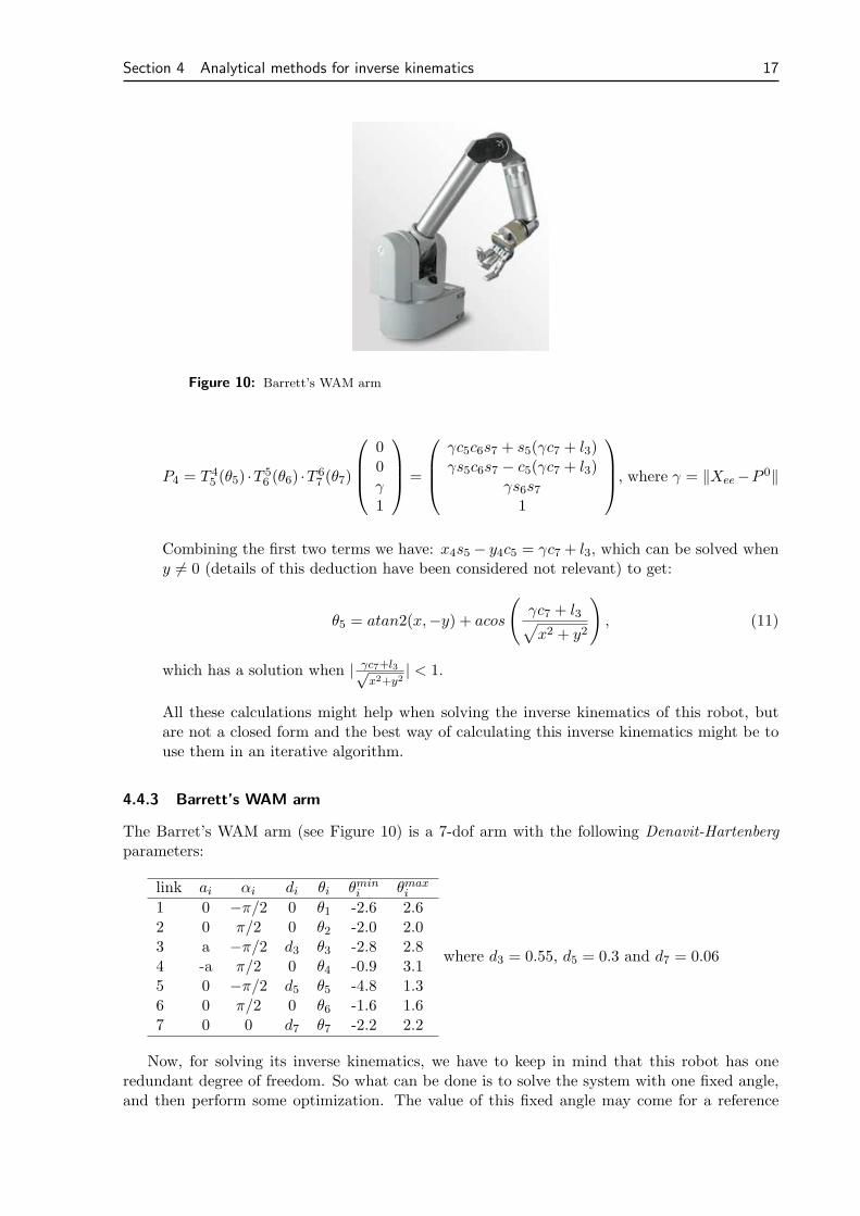
Figure 10: Barrett’s WAM arm
P4 = T 45 (θ5) ·T 5
6 (θ6) ·T 67 (θ7)
00γ1
=
γc5c6s7 + s5(γc7 + l3)γs5c6s7 − c5(γc7 + l3)
γs6s71
, where γ = ‖Xee−P 0‖
Combining the first two terms we have: x4s5 − y4c5 = γc7 + l3, which can be solved wheny 6= 0 (details of this deduction have been considered not relevant) to get:
θ5 = atan2(x,−y) + acos
(
γc7 + l3√
x2 + y2
)
, (11)
which has a solution when | γc7+l3√x2+y2
| < 1.
All these calculations might help when solving the inverse kinematics of this robot, butare not a closed form and the best way of calculating this inverse kinematics might be touse them in an iterative algorithm.
4.4.3 Barrett’s WAM arm
The Barret’s WAM arm (see Figure 10) is a 7-dof arm with the following Denavit-Hartenbergparameters:
link ai αi di θi θmini θmax
i
1 0 −π/2 0 θ1 -2.6 2.62 0 π/2 0 θ2 -2.0 2.03 a −π/2 d3 θ3 -2.8 2.84 -a π/2 0 θ4 -0.9 3.15 0 −π/2 d5 θ5 -4.8 1.36 0 π/2 0 θ6 -1.6 1.67 0 0 d7 θ7 -2.2 2.2
where d3 = 0.55, d5 = 0.3 and d7 = 0.06
Now, for solving its inverse kinematics, we have to keep in mind that this robot has oneredundant degree of freedom. So what can be done is to solve the system with one fixed angle,and then perform some optimization. The value of this fixed angle may come for a reference
18 Master Thesis
position, such as could be a rest position, or just the previous position in a trajectory to beperformed.
It is also relevant in this robot that the last 3 dof consist of a Spherical wrist, which can thenbe treated independently. So to compute the inverse kinematics of the robot given a desiredhomogeneous transformation:
Tobj =
(
Rx Ry Rz Pobj
0 0 0 1
)
, (12)
we can consider the spherical wrist center as Pw = Pobj − d7 ·Rz.This reduces the 7-variable problem to a 4-dof positioning problem, where the task is to
reach point Pw (dimension 3), without paying attention (a priori) to the orientation of the endeffector.
Now, back to the problem, we have a 4 dof robot with a 3-D task. And the first question toask is which angle to fix to calculate a first solution.
When looking at the robot, one might think that the closest angle to represent the redun-dancy of this robot might be θ3. But in fact, after comparing the solutions of fixing any ofthe first 3 joints, it has been concluded that the best joint to be fixed when solving the inversekinematics is the first one, mainly because it moves all the inertia of the robot, and minimizingits angle variation will reduce the total energy in a movement.
First, we can compute the angle θ4 with the equation of the distance from the origin to thespherical wrist point:
‖P 0w‖2 = ‖T 0
1 (θ1) · T 12 (θ2) · T 2
3 (θ3) · T 34 (θ4)‖2 = ...
= d23 + d25 + d27 + 2(d5 · a+ a · d3)sin(θ4) + 2(d3 · d5 + a2)cos(θ4),
which can be solved to obtain two possible values of θ4, called inner elbow and outer elbowconfigurations, depending on the sign of θ4.
And then, knowing that P 4w =
000.31
, we can express
T 23 (θ3)T
43 (θ4) · P 4
w = (T 12 (θ2))
−1(T 10 (θ1))
−1 · P 0w :
0.3 c3s4 − 9200 c3c4 +
9200 c3
0.3 s3s4 − 9200 s3c4 +
9200 s3
1120 + 0.3 c4 +
9200 s4
1.0
=
=
s1c2(P0w )x + s1c2(P
0w )y − s2(P
0w )z
−s1(P0w )x + c1(P
0w )y
c1s2(P0w )x + s1s2(P
0w )y + c2(P
0w )z
1
,
from where, knowing θ1 and θ4, we can obtain the two solutions of θ2 by solving:
1120 + 0.3 c4 +
9200 s4
= c1s2(P0w )x + s1s2(P
0w )y + c2(P
0w )z
(13)
and, with θ2, we obtain c3 = cos(θ3):
Section 4 Analytical methods for inverse kinematics 19
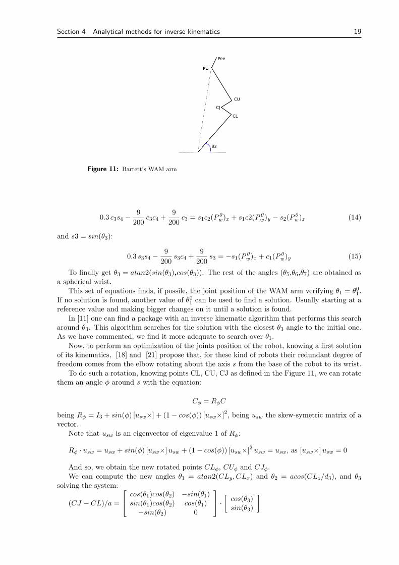
CU
CJ
CL
Pw
Pee
θ2
Figure 11: Barrett’s WAM arm
0.3 c3s4 −9
200c3c4 +
9
200c3 = s1c2(P
0w )x + s1c2(P
0w )y − s2(P
0w )z (14)
and s3 = sin(θ3):
0.3 s3s4 −9
200s3c4 +
9
200s3 = −s1(P
0w )x + c1(P
0w )y (15)
To finally get θ3 = atan2(sin(θ3),cos(θ3)). The rest of the angles (θ5,θ6,θ7) are obtained asa spherical wrist.
This set of equations finds, if possile, the joint position of the WAM arm verifying θ1 = θ01.If no solution is found, another value of θ01 can be used to find a solution. Usually starting at areference value and making bigger changes on it until a solution is found.
In [11] one can find a package with an inverse kinematic algorithm that performs this searcharound θ3. This algorithm searches for the solution with the closest θ3 angle to the initial one.As we have commented, we find it more adequate to search over θ1.
Now, to perform an optimization of the joints position of the robot, knowing a first solutionof its kinematics, [18] and [21] propose that, for these kind of robots their redundant degree offreedom comes from the elbow rotating about the axis s from the base of the robot to its wrist.
To do such a rotation, knowing points CL, CU, CJ as defined in the Figure 11, we can rotatethem an angle φ around s with the equation:
Cφ = RφC
being Rφ = I3 + sin(φ) [usw×] + (1− cos(φ)) [usw×]2, being usw the skew-symetric matrix of avector.
Note that usw is an eigenvector of eigenvalue 1 of Rφ:
Rφ · usw = usw + sin(φ) [usw×]usw + (1− cos(φ)) [usw×]2 usw = usw, as [usw×]usw = 0
And so, we obtain the new rotated points CLφ, CUφ and CJφ.
We can compute the new angles θ1 = atan2(CLy, CLx) and θ2 = acos(CLz/d3), and θ3solving the system:
(CJ − CL)/a =
cos(θ1)cos(θ2) −sin(θ1)sin(θ1)cos(θ2) cos(θ1)
−sin(θ2) 0
·[
cos(θ3)sin(θ3)
]
20 Master Thesis
00.10.20.30.40 0.1 0.2 0.3 0.4
0
0.05
0.1
0.15
0.2
0.25
0.3
0.35
0.4
0.45
0.5
x
WAM arm redundant degree of freedom optimization
y
z
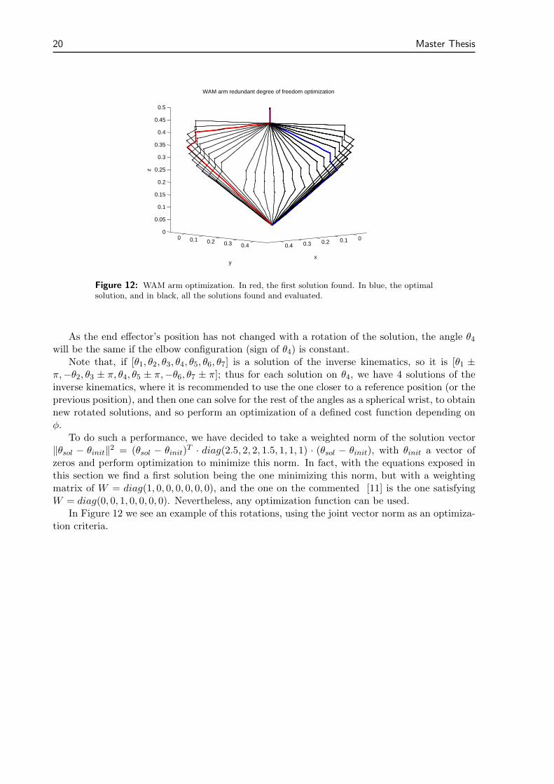
Figure 12: WAM arm optimization. In red, the first solution found. In blue, the optimalsolution, and in black, all the solutions found and evaluated.
As the end effector’s position has not changed with a rotation of the solution, the angle θ4will be the same if the elbow configuration (sign of θ4) is constant.
Note that, if [θ1, θ2, θ3, θ4, θ5, θ6, θ7] is a solution of the inverse kinematics, so it is [θ1 ±π,−θ2, θ3 ± π, θ4, θ5 ± π,−θ6, θ7 ± π]; thus for each solution on θ4, we have 4 solutions of theinverse kinematics, where it is recommended to use the one closer to a reference position (or theprevious position), and then one can solve for the rest of the angles as a spherical wrist, to obtainnew rotated solutions, and so perform an optimization of a defined cost function depending onφ.
To do such a performance, we have decided to take a weighted norm of the solution vector‖θsol − θinit‖2 = (θsol − θinit)
T · diag(2.5, 2, 2, 1.5, 1, 1, 1) · (θsol − θinit), with θinit a vector ofzeros and perform optimization to minimize this norm. In fact, with the equations exposed inthis section we find a first solution being the one minimizing this norm, but with a weightingmatrix of W = diag(1, 0, 0, 0, 0, 0, 0), and the one on the commented [11] is the one satisfyingW = diag(0, 0, 1, 0, 0, 0, 0). Nevertheless, any optimization function can be used.
In Figure 12 we see an example of this rotations, using the joint vector norm as an optimiza-tion criteria.
Section 5 Time-discrete control-based methods 21
5 Time-discrete control-based methods
Sometimes it is not possible to find a closed-form analytical solution to the inverse kinematicproblem of a manipulator, and this becomes even harder in the case of a redundant manipulator,where infinite solutions may exist, forming a subset of the joint space. In these cases, controlmethods are often applied to solve the problem of the inverse kinematics of the manipulator.
In this section, we analyse the state of the art on inverse kinematics with control methods,commenting the advantages and disadvantages of the different methods on the literature, andwe try to find a method which is robust when handling joint limits, convergence issues andsingularities.
We must point out that all these methods are first-order derivative methods, whose systemsare linear. There are also other linear methods such as the extended Jacobian (proposed initiallyby Baillieul [1] and further developed in [9]), which are not considered here because of theirneed to compute the 2nd order Jacobian, which makes the computational complexity of themethod grow.
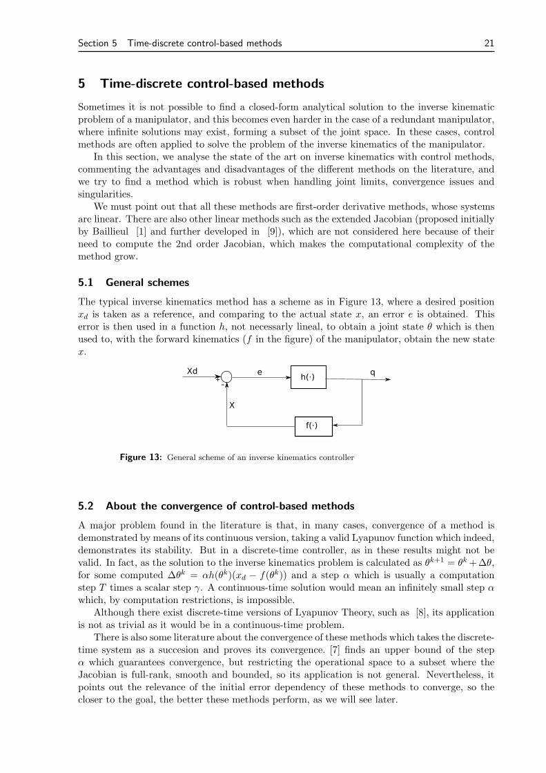
5.1 General schemes
The typical inverse kinematics method has a scheme as in Figure 13, where a desired positionxd is taken as a reference, and comparing to the actual state x, an error e is obtained. Thiserror is then used in a function h, not necessarly lineal, to obtain a joint state θ which is thenused to, with the forward kinematics (f in the figure) of the manipulator, obtain the new statex.
Xd
X
e+-
q
f(·)
h(·)
Figure 13: General scheme of an inverse kinematics controller
5.2 About the convergence of control-based methods
A major problem found in the literature is that, in many cases, convergence of a method isdemonstrated by means of its continuous version, taking a valid Lyapunov function which indeed,demonstrates its stability. But in a discrete-time controller, as in these results might not bevalid. In fact, as the solution to the inverse kinematics problem is calculated as θk+1 = θk+∆θ,for some computed ∆θk = αh(θk)(xd − f(θk)) and a step α which is usually a computationstep T times a scalar step γ. A continuous-time solution would mean an infinitely small step αwhich, by computation restrictions, is impossible.
Although there exist discrete-time versions of Lyapunov Theory, such as [8], its applicationis not as trivial as it would be in a continuous-time problem.
There is also some literature about the convergence of these methods which takes the discrete-time system as a succesion and proves its convergence. [7] finds an upper bound of the stepα which guarantees convergence, but restricting the operational space to a subset where theJacobian is full-rank, smooth and bounded, so its application is not general. Nevertheless, itpoints out the relevance of the initial error dependency of these methods to converge, so thecloser to the goal, the better these methods perform, as we will see later.
22 Master Thesis
The problem of finding a step which, on the one hand, ensures convergence and, on the otherhand, gives an acceptable computational cost, is then an issue to focus on.
Using first order derivative methods of the robot’s motion has the drawback that, dependingon the method and the goal position, an algorithm can get stuck at an algorithmic singularity,which is when we arrive at a point where the error e belongs to the kernel of the invertedJacobian, or in a multiple-task method, a secondary task joint variation takes the contraryvalue of the primary task.
5.3 Methods from literature
In the next sections, we will describe different control-based methodologies for obtaining theinverse kinematics, we will apply them to a simple robot such as a 4R with all joint limits setat [−π/2, π/2]. Most of the methods are based on the pseudoinverse of the Jacobian. Withthis, one may ask why not using J−1. In fact, the inverse matrix does not exist for a non-squared or non-full ranked matrices and also its terms tend to infinite as the matrix approachesa singularity. To our criteria, we will mainly prioritize the following:
• Desired position convergence.
• Joint limit avoidance.
• Robustness when a singularity occurs.
• Computational cost.
From now on, a set of methods will be described. For each of them, we will first explainits main idea intuitively, and then present its algorithm, to later on show their behaviour withexamples and comment their advantages and disadvantages. To illustrate, we will use a 4R planarrobot for a positioning 2-dimensional task, which gives a remaining of 2 redundant degrees offreedom with the following Denavit-Hartenberg parameters:
link ai(m) αi di θi θmini θmax
i
1 0.4 0 0 θ1 0 02 0.3 0 0 θ2 0 03 0.2 0 0 θ3 0 04 0.1 0 0 θ4 0 0
To start, we will present the two most simple methods: the Jacobian pseudoinverse and theJacobian transposed. We will comment their drawbacks, and we will present some variationsover those methods so as to reduce the effect of their main concerns, which are:
• Jacobian with very small eigenvalues (singularities). To solve this problem, thetypical solution applied is to damp or filter the Jacobian matrix when calculating itsinverse, or even damp selectively according to the joint’s movements.
• Secondary tasks. When possible, secondary tasks, apart from reaching the goal can beadded to an algorithm. To this purpose, we present the gradient projection method, itsgeneralisation, the task-priority methods, and also the Jacobian weighting methods.
• Joint limit avoidance. To avoid joint limits, apart from considering it as a secondarytask or even a primary one, joints can be blocked when necessary. This can lead to adiscontinuous activation and deactivation of blocking tasks, so a continuous clamping isalso presented.
Section 5 Time-discrete control-based methods 23
5.3.1 Jacobian pseudoinverse
The Jacobian pseudoinverse method consists in directly inverting the matrix J in the first-orderdifferential equation x = Jθ (discretized as ∆x = e = J∆θ. The point is that, on redundantmanipulators, J is not a square matrix, so a more general inverse matrix, called Moore-Penrosepseudoinverse, is used so as to invert J and solve the problem. This inverse operator has alsothe property to give the least-squares minimum norm solution. so the solution ∆θ gives theminimum value of ‖J∆θ − e‖.
As we have just said, the Jacobian pseudoinverse method is based on the Moore-Penrosepseudoinverse matrix, which is defined as J† = JT · (J · JT )−1 when J · JT is invertible. Fornon full row rank matrices, the pseudoinverse is defined more generally as the matrix verifyingJJ†J = J .
With this matrix, we define the method as:
∆θ = α · J† · e,
being α the method step, J† the pseudoinverse of the geometric Jacobian of the manipulator,and e the task error.
In some cases, when a robot is in a singularity, the method might get stuck in a point or havetoo large values on the pseudoinverse matrix. This can be easily seen if we take the formula ofthe Jacobian pseudoinverse matrix: J† = JT · (J · JT )−1. If the Jacobian matrix is close to asingularity, then J ·JT will have very small terms, which will translate to very large terms wheninverting the matrix.
To verify that, if we take the singular value decomposition of J :
J = U · Σ · V T , (16)
where U, V are orthonormal matrices (if J is n × m, being m the number of joints and n thetask space dimension, then U is m × m and V is n × n) and Σ is a diagonal m × n matrixwith σi its diagonal elements, where σ1 ≥ σ2 ≥ ... ≥ σm ≥ 0. (Note that σi may be zero if J isrank-deficient).
Then if we define r = maxi{i | σi > 0}, we have that r = rank(J), and we can write(considering m ≥ n):
J =m∑
i=1σiuiv
Ti =
r∑
i=1σiuiv
Ti , with ui and vi being the ith columns of U and V, respectively.
Now, as U and V are orthonormal matrices, we can compute the pseudoinverse of J as
J† = V · Σ† · UT =r∑
i=1
1σiviu
Ti .
With this expression of the Jacobian pseudoinverse, we clearly see that when the robot getsclose to a singularity, one σj becomes very small and so 1
σjcan be very large. As limσj→0
1σj
= ∞,
this implies very large gains when computing ∆θ = J† · e.With this representation, the reconstruction error of the method, i.e. the difference between
the error and the variation of position in the task space, at a differential level, can be expressed,for α = 1 as [4]:
xe − J · q =m∑
i=r+1
uTi ·xe
σivi.
Now we will show the results of the pseudoinverse method, using the scheme ∆θ = J†e, witha step α = 1.
The three results shown are those obtained in a planar 4R robot, with a position tracking
24 Master Thesis
−0.2 0 0.2 0.4 0.6 0.8 1 1.20
0.1
0.2
0.3
0.4
0.5
0.6
0.7
0.8
0.9
1
x
y
Trajectory
1 1.5 2 2.5 3 3.5 4 4.5 5 5.5 6−2
−1.5
−1
−0.5
0
0.5
1
1.5
2
iteration
qi (
rad)
Joint trajectory
q1
q2
q3
q4
1 1.5 2 2.5 3 3.5 4 4.5 5 5.5 60
0.5
1
1.5Absolute Error
x errory errorerror norm
Jacobian Pseudoinverse, Vertical singularity end, step=1
1 1.5 2 2.5 3 3.5 4 4.5 50
0.2
0.4
0.6
0.8
1
1.2
1.4
1.6
1.8
2Step
Figure 14: Behaviour of the pseudoinverse method in a singular objective. On the upperleft plot, the green line shows the evolution of end effector’s position, while the robotstructure is drawn evolving from yellow to blue.
(not considering orientation) for an initial configuration of θ =
0000
and three different desired
configurations, with a tolerated error of 1 cm. This error might be considered too high for realtasks, but we have considered it is small enough to these illustration purposes.
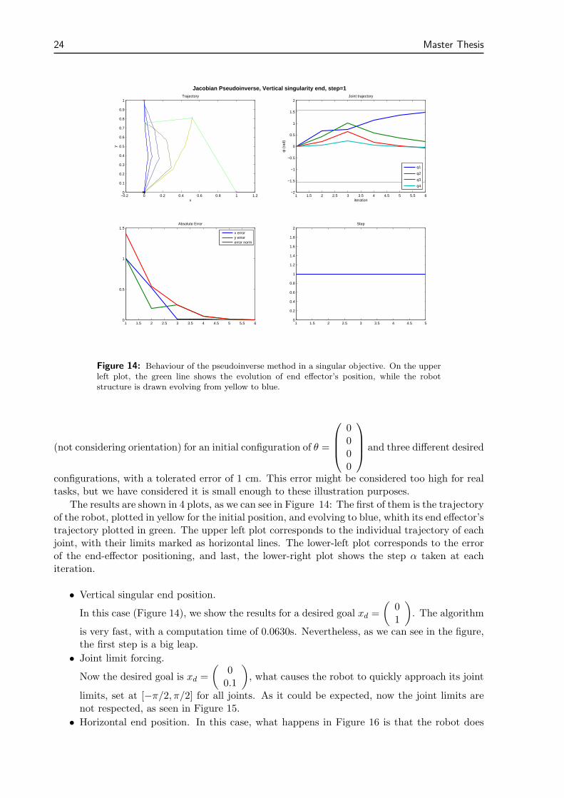
The results are shown in 4 plots, as we can see in Figure 14: The first of them is the trajectoryof the robot, plotted in yellow for the initial position, and evolving to blue, whith its end effector’strajectory plotted in green. The upper left plot corresponds to the individual trajectory of eachjoint, with their limits marked as horizontal lines. The lower-left plot corresponds to the errorof the end-effector positioning, and last, the lower-right plot shows the step α taken at eachiteration.
• Vertical singular end position.
In this case (Figure 14), we show the results for a desired goal xd =
(
01
)
. The algorithm
is very fast, with a computation time of 0.0630s. Nevertheless, as we can see in the figure,the first step is a big leap.
• Joint limit forcing.
Now the desired goal is xd =
(
00.1
)
, what causes the robot to quickly approach its joint
limits, set at [−π/2, π/2] for all joints. As it could be expected, now the joint limits arenot respected, as seen in Figure 15.
• Horizontal end position. In this case, what happens in Figure 16 is that the robot does
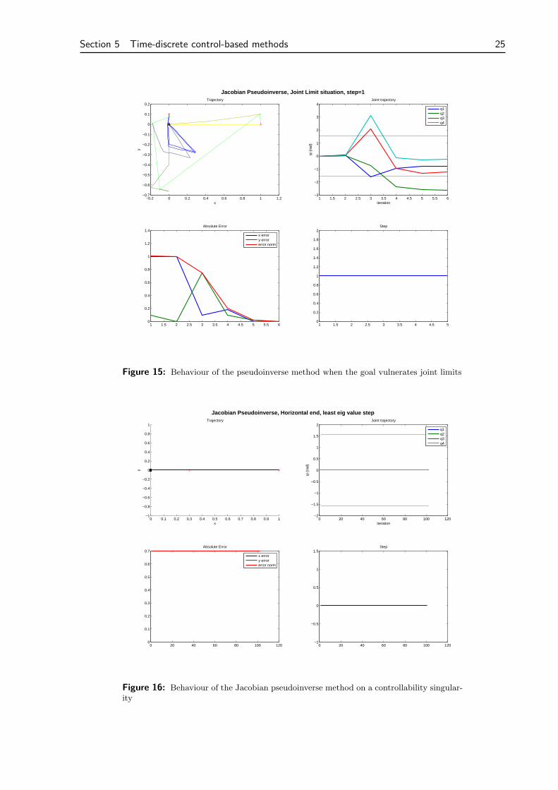
Section 5 Time-discrete control-based methods 25
−0.2 0 0.2 0.4 0.6 0.8 1 1.2−0.7
−0.6
−0.5
−0.4
−0.3
−0.2
−0.1
0
0.1
0.2
x
y
Trajectory
1 1.5 2 2.5 3 3.5 4 4.5 5 5.5 6−3
−2
−1
0
1
2
3
4
iteration
qi (
rad)
Joint trajectory
q1q2q3q4
1 1.5 2 2.5 3 3.5 4 4.5 5 5.5 60
0.2
0.4
0.6
0.8
1
1.2
1.4Absolute Error
x errory errorerror norm
Jacobian Pseudoinverse, Joint Limit situation, step=1
1 1.5 2 2.5 3 3.5 4 4.5 50
0.2
0.4
0.6
0.8
1
1.2
1.4
1.6
1.8
2Step
Figure 15: Behaviour of the pseudoinverse method when the goal vulnerates joint limits
0 0.1 0.2 0.3 0.4 0.5 0.6 0.7 0.8 0.9 1−1
−0.8
−0.6
−0.4
−0.2
0
0.2
0.4
0.6
0.8
1Trajectory
x
y
0 20 40 60 80 100 120−2
−1.5
−1
−0.5
0
0.5
1
1.5
2
iteration
qi (
rad)
Joint trajectory
q1q2q3q4
0 20 40 60 80 100 1200
0.1
0.2
0.3
0.4
0.5
0.6
0.7Absolute Error
x errory errorerror norm
Jacobian Pseudoinverse, Horizontal end, least eig value step
0 20 40 60 80 100 120−1
−0.5
0
0.5
1
1.5Step
Figure 16: Behaviour of the Jacobian pseudoinverse method on a controllability singular-ity
26 Master Thesis
−0.2 0 0.2 0.4 0.6 0.8 1 1.20
0.1
0.2
0.3
0.4
0.5
0.6
0.7
0.8
0.9
1
x
y
Trajectory
0 20 40 60 80 100 120 140−2
−1.5
−1
−0.5
0
0.5
1
1.5
2
iteration
qi (
rad)
Joint trajectory
q1q2q3q4
0 20 40 60 80 100 120 1400
0.5
1
1.5Absolute Error
x errory errorerror norm
Jacobian Transpose, Vertical singularity end, normalised error step
0 20 40 60 80 100 120 1400.5
1
1.5
2
2.5
3
3.5Step
Figure 17: Behaviour of the Jacobian transpose method when the goal is a singular po-sition
not move at all. The Jacobian matrix in this case has the form J = [ 0 v ] and the errorvector e = [ex 0]T . When we calculate the pseudoinverse of J , it only has rank 1 so itsproduct with e is 0 and the robot won’t move.
5.3.2 Jacobian transpose
To gain speed, the Jacobian transpose method uses, instead of an inverse of the matrix J, itstranspose. This might be compared as if we were considering matrix J as a kind of orthonormalmatrix. Nevertheless, it can be proved in terms of Lypaunov theorem that, for a sufficiently smallstep α, the control scheme converges to zero error.
As said, now the control rule using the scheme in Figure 13 is: ∆θ = αJT e ,where JT is nowthe transpose of the geometric Jacobian of the manipulator.
This method is computationally very fast step by step, although it may require more stepsthan other methods, and it does not consider joint limits.
When choosing α, some literature recommend taking the value that would make the norm
of the change in the task space equal to the norm of the error. That is α = <JJT e,e><JJT e,JJT e>
.Now we will show some examples of the behaviour of this method for the mentioned 4R
manipulator, using (with < ·, · > the dot product):
∆θ =< JJT e, e >
< JJT e, JJT e >JT e. (17)
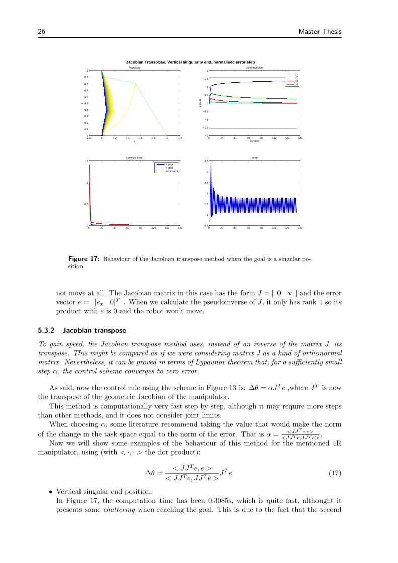
• Vertical singular end position.In Figure 17, the computation time has been 0.3085s, which is quite fast, althought itpresents some chattering when reaching the goal. This is due to the fact that the second
Section 5 Time-discrete control-based methods 27
−0.2 0 0.2 0.4 0.6 0.8 1 1.20
0.1
0.2
0.3
0.4
0.5
0.6
0.7
0.8
x
y
Trajectory
0 2 4 6 8 10 12 14−2
−1.5
−1
−0.5
0
0.5
1
1.5
2
2.5
iteration
qi (
rad)
Joint trajectory
q1
q2
q3
q4
0 2 4 6 8 10 12 140
0.2
0.4
0.6
0.8
1
1.2
1.4Absolute Error
x errory errorerror norm
Jacobian Transpose, Joint Limit situation, normalised error step
0 2 4 6 8 10 120
2
4
6
8
10
12
14
16
18Step
Figure 18: Behaviour of the Jacobian transpose method when the objective vulneratesjoint limits
row of the Jacobian matrix has very small values, compared to the first row, as the robotapproaches the singularity on the goal, so a gain on vertical position implies more variationin the horizontal direction. This chattering makes the algorithm find the solution muchslower, loosing the computational speed gained in avoiding to invert the Jacobian matrix.
• Joint limit forcing.In Figure 18, we see that, as the Jacobian transposed method does not take into accountjoint limits, those are easily surpassed.What could be done to avoid surpassing these joint limits is to assign the maximum orminimum value for the joint if it is surpassed, but this does not work well, as the joint isforced to keep moving towards the joint limit and it gets blocked, possibly blocking theother joints, as we can see in Figure 19.
• Horizontal end position.Now the same problem as with the Jacobian pseudoinverse method happens when thehorizontal position is the goal, avoiding the robot to move in that direction.
5.3.3 Jacobian damping and filtering
As commented on the Jacobian pseudoinverse method, when close to a singularity, the pseu-doinverse method can have very large gains. In addition, the pseudoinverse operator has adiscontinuity w.r.t. the eigenvalues of J in σ = 0. To avoid this discontinuity and reduce theselarge gains, which imply a large condition number of the Jacobian, meaning numerical error, theJacobian pseudoinverse can be damped.
There are some ways of trying to avoid discontinuities on the singularities, such as damp-ing/filtering the Jacobian matrix, a good view of these methods can be found in [6] and [4].

28 Master Thesis
−0.2 0 0.2 0.4 0.6 0.8 1 1.20
0.1
0.2
0.3
0.4
0.5
0.6
0.7
0.8
x
y
Trajectory
0 100 200 300 400 500 600−2
−1.5
−1
−0.5
0
0.5
1
1.5
2
iteration
qi (
rad)
Joint trajectory
q1q2q3q4
0 100 200 300 400 500 6000
0.2
0.4
0.6
0.8
1
1.2
1.4Absolute Error
x errory errorerror norm
Jacobian Transpose, Joint Limit blocking situation, normalised error step
0 100 200 300 400 500 6000
1
2
3
4
5
6
7
8Step
Figure 19: Behaviour of the Jacobian transpose method with joints being blocked at theirlimits
• Jacobian damping. If we take an alternative expression of the pseudoinverse, called
damped pseudoinverse, defined as: J † = J · (JJT + λ2I)−1 =r∑
i=1
σi
σ2
i +λ2viu
Ti
which is, for some small λ, almost the same matrix as the ordinary pseudoinverse whenσ2i ≫ λ2 ∀i, and when some σj is close to zero, limσj→0
σi
σ2
i +λ2= 0, instead of ∞.
This avoids the large gains commented, but also adds a chattering to the solution whenclose to a singularity. This chattering must be avoided, commonly picking a very smallvalue of λ, as the new reconstruction error will be, for α = 1
xe − J · q =r∑
i=1λ2 (u
Ti xe)−σi(v
Ti q0)
σ2
i +λ2vi +
m∑
i=r+1
uTi ·xe
σivi
which evidentiates the possible need of varying the damping factor λ, as it adds a newerror. This is also commented in [6].
Now, testing this method on the 4R manipulator: ∆θ = αJ ·(JJT+λ2I)−1e = αr∑
i=1
σi
σ2
i +λ2viu
Ti e
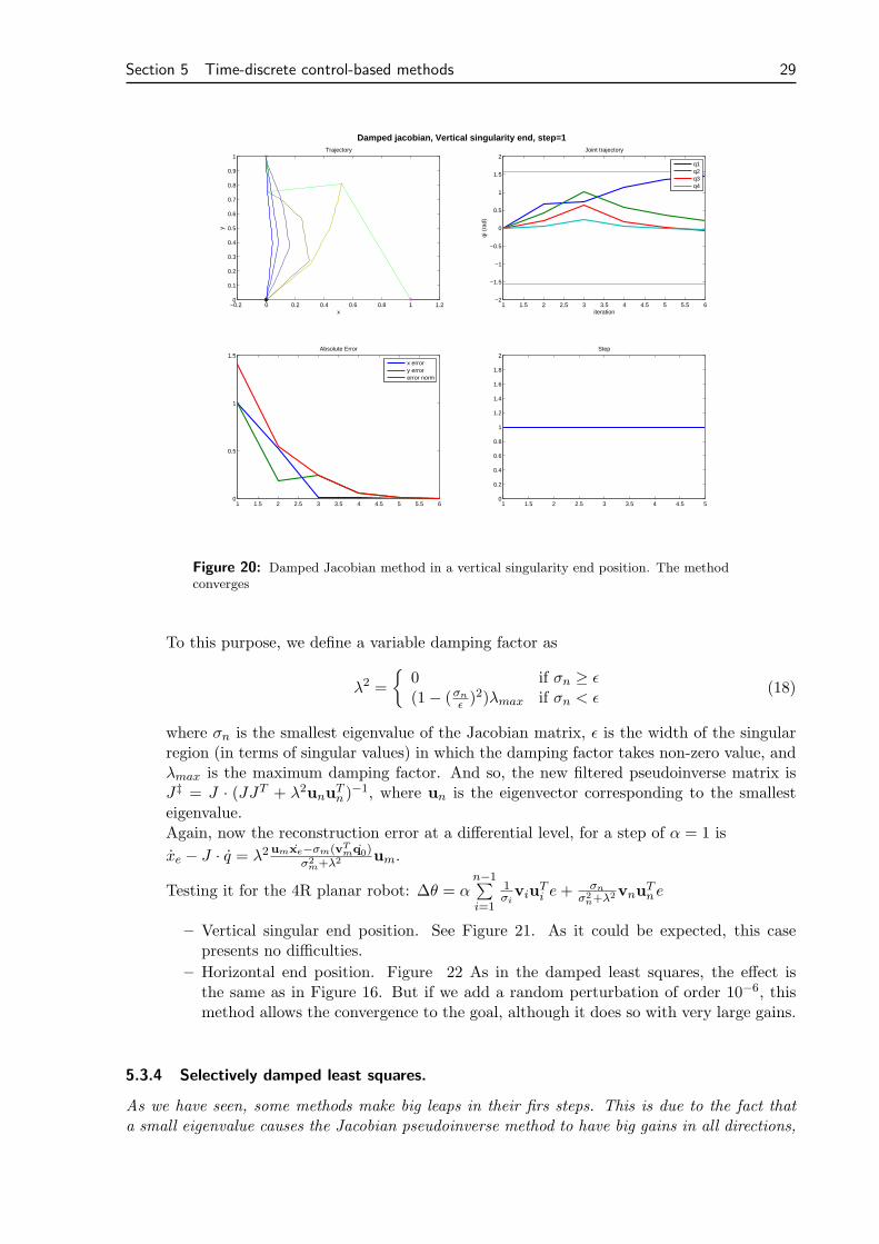
– Vertical singular end position, as seen in Figure 20, with a computation time of0.0525s. The method presents no problems as expected.
– Horizontal end position. The same as in Figure 16 happens. This is due to the factthat the damping is effective in a neighbourhood of a singularity, but, looking at thesingular value decomposition of the method, we can see that σi
σ2
i +λ2= 0 for σi = 0.
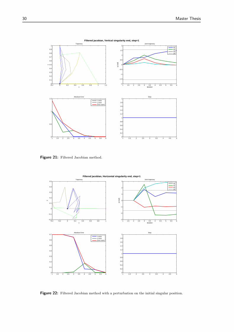
• Numerical filtering. A way of reducing the mentioned reconstruction error in the Ja-cobian damping methods is to define a singular region and apply the damping factor onlywhen entering it [5].
Section 5 Time-discrete control-based methods 29
−0.2 0 0.2 0.4 0.6 0.8 1 1.20
0.1
0.2
0.3
0.4
0.5
0.6
0.7
0.8
0.9
1
x
y
Trajectory
1 1.5 2 2.5 3 3.5 4 4.5 5 5.5 6−2
−1.5
−1
−0.5
0
0.5
1
1.5
2
iteration
qi (
rad)
Joint trajectory
q1q2q3q4
1 1.5 2 2.5 3 3.5 4 4.5 5 5.5 60
0.5
1
1.5Absolute Error
x errory errorerror norm
Damped jacobian, Vertical singularity end, step=1
1 1.5 2 2.5 3 3.5 4 4.5 50
0.2
0.4
0.6
0.8
1
1.2
1.4
1.6
1.8
2Step
Figure 20: Damped Jacobian method in a vertical singularity end position. The methodconverges
To this purpose, we define a variable damping factor as
λ2 =
{
0 if σn ≥ ǫ(1− (σn
ǫ )2)λmax if σn < ǫ(18)
where σn is the smallest eigenvalue of the Jacobian matrix, ǫ is the width of the singularregion (in terms of singular values) in which the damping factor takes non-zero value, andλmax is the maximum damping factor. And so, the new filtered pseudoinverse matrix isJ‡ = J · (JJT + λ2unu
Tn )
−1, where un is the eigenvector corresponding to the smallesteigenvalue.Again, now the reconstruction error at a differential level, for a step of α = 1 is
xe − J · q = λ2 umxe−σm(vTmq0)
σ2m+λ2 um.
Testing it for the 4R planar robot: ∆θ = αn−1∑
i=1
1σiviu
Ti e+
σn
σ2n+λ2vnu
Tne
– Vertical singular end position. See Figure 21. As it could be expected, this casepresents no difficulties.
– Horizontal end position. Figure 22 As in the damped least squares, the effect isthe same as in Figure 16. But if we add a random perturbation of order 10−6, thismethod allows the convergence to the goal, although it does so with very large gains.
5.3.4 Selectively damped least squares.
As we have seen, some methods make big leaps in their firs steps. This is due to the fact thata small eigenvalue causes the Jacobian pseudoinverse method to have big gains in all directions,
30 Master Thesis
−0.2 0 0.2 0.4 0.6 0.8 1 1.20
0.1
0.2
0.3
0.4
0.5
0.6
0.7
0.8
0.9
1
x
y
Trajectory
1 1.5 2 2.5 3 3.5 4 4.5 5 5.5 6−2
−1.5
−1
−0.5
0
0.5
1
1.5
2
iteration
qi (
rad)
Joint trajectory
q1q2q3q4
1 1.5 2 2.5 3 3.5 4 4.5 5 5.5 60
0.5
1
1.5Absolute Error
x errory errorerror norm
Filtered jacobian, Vertical singularity end, step=1
1 1.5 2 2.5 3 3.5 4 4.5 50
0.2
0.4
0.6
0.8
1
1.2
1.4
1.6
1.8
2Step
Figure 21: Filtered Jacobian method.
−0.4 −0.2 0 0.2 0.4 0.6 0.8 1−0.2
−0.1
0
0.1
0.2
0.3
0.4
0.5
x
y
Trajectory
1 1.5 2 2.5 3 3.5 4 4.5 5 5.5 6−3
−2
−1
0
1
2
3
iteration
qi (
rad)
Joint trajectory
q1q2q3q4
1 1.5 2 2.5 3 3.5 4 4.5 5 5.5 60
0.1
0.2
0.3
0.4
0.5
0.6
0.7Absolute Error
x errory errorerror norm
Filtered jacobian, Horizontal singularity end, step=1
1 1.5 2 2.5 3 3.5 4 4.5 50
0.2
0.4
0.6
0.8
1
1.2
1.4
1.6
1.8
2Step
Figure 22: Filtered Jacobian method with a perturbation on the initial singular position.

Section 5 Time-discrete control-based methods 31
even if these small eigenvalues are damped or filtered. In [2], a new way of damping is defined,which consists in damping differently the effect of each one of the components of the positionerror, expressed in the base of the singular value decomposition of J , so small eigenvalues of theJacobian, which would turn into large gains, are damped more severely.
First, consider the singular value decomposition of the Jacobian matrix, and the pseudoin-verse algorithm:
J = UΣV T =n∑
j=1
uiσivTi .
∆θ = J†e =
n∑
j=1
σ−1i viu
Ti e,
where ui are the eigenvectors of J in the task space.
Then if we consider a unitary error in the direction of one of the eigenvectors in the taskspace (columns of U), e = ui, then the pseudoinverse method would give a variation of joint jof ∆θj = σ−1
i vj,i(uTi ·ui) = σ−1
i vj,i, which translates in a movement of the robot in the directionof ui of σ
−1i vj,iJj , being Jj the jth column of the Jacobian matrix. Thus it is defined:
Mi = σ−1i
m∑
j=1
|vj,i|‖Jj‖, (19)
where Jj is the jth column of the Jacobian matrix of the manipulator, and Mi estimates thesum of the distances moved by the end effector caused by the individual changes in joint angles.
Now, defining a maximum angle change γmax, we can bound the angle change in responseto the ith component (in base U) of the error e as:
γi = min(1, 1/Mi)γmax.
The idea is that, whenMi is small, the joints’ changes of each error component have cancelledeach other, and so a higher response is needed, but only in the affected direction (ui), as withthe pseudoinverse method the same gain is applied to all coordinates.
Now this γi is used to damp the gain on each column of matrix U
∆qi =
{
wi if ‖wi‖∞ ≤ γiγi
wi
‖wi‖∞otherwise
being wi = σ−1i vi(u
Ti · e) (wi = 0 in case σi = 0)
And finally damping the total motion by
∆θ =
{
∆θ if ‖∆θ‖∞ ≤ γmax
γmax∆θ
‖∆θ‖∞otherwise
Where ∆θ =∑
i|σi 6=0
∆qi
Now, using this method with a 4R planar robot, we have:
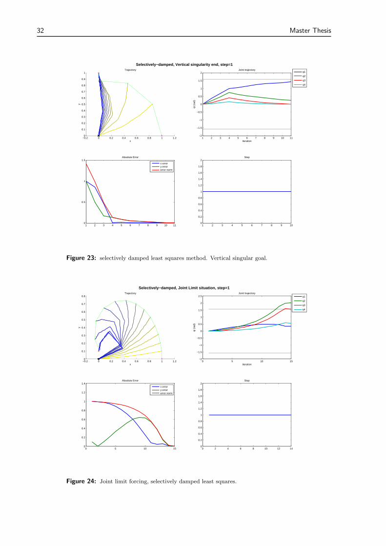
• Vertical singular end position. Computation time of 0.0642s. As we can see in Figure 23,the method converges fastly, and smoothly.
• Joint limit forcing. (Computation time of 0.0890s) Although the steps are very uniform,as we can see in Figure 24, joint limits are not respected because they are not consideredin the algorithm.
• Horizontal end position. In this case, it also happens to be that the initial error belongsto the kernel of the algorithm, so the robot won’t move as in Figure 16.
32 Master Thesis
−0.2 0 0.2 0.4 0.6 0.8 1 1.20
0.1
0.2
0.3
0.4
0.5
0.6
0.7
0.8
0.9
1Trajectory
x
y
1 2 3 4 5 6 7 8 9 10 11−2
−1.5
−1
−0.5
0
0.5
1
1.5
2
iteration
qi (
rad)
Joint trajectory
q1
q2
q3
q4
1 2 3 4 5 6 7 8 9 10 110
0.5
1
1.5Absolute Error
x errory errorerror norm
Selectively−damped, Vertical singularity end, step=1
1 2 3 4 5 6 7 8 9 100
0.2
0.4
0.6
0.8
1
1.2
1.4
1.6
1.8
2Step
Figure 23: selectively damped least squares method. Vertical singular goal.
−0.2 0 0.2 0.4 0.6 0.8 1 1.20
0.1
0.2
0.3
0.4
0.5
0.6
0.7
0.8Trajectory
x
y
0 5 10 15−2
−1.5
−1
−0.5
0
0.5
1
1.5
2
2.5
iteration
qi (
rad)
Joint trajectory
q1
q2
q3
q4
0 5 10 150
0.2
0.4
0.6
0.8
1
1.2
1.4Absolute Error
x errory errorerror norm
Selectively−damped, Joint Limit situation, step=1
0 2 4 6 8 10 12 140
0.2
0.4
0.6
0.8
1
1.2
1.4
1.6
1.8
2Step
Figure 24: Joint limit forcing, selectively damped least squares.
Section 5 Time-discrete control-based methods 33
5.3.5 Gradient projection
With the pseudoinverse method, we find the solution of the least-squares problem. Nevertheless,when having redundant degrees of freedom, we can optimize according to another criterion, andone way of doing so without altering much the zero-error tracking is to create a secondary taskas a gradient of a function, and projecting to the kernel of the primary task.
When we have a redundant manipulator, we can add a secondary objective to the solutionof the inverse kinematics. An easy way of doing so is to create a cost function H, calculate itsgradient ∇H, and project it to the kernel of the matrix J . Why projecting into the kernel ofJ? Knowing that for any position of the manipulator, x = J · q, this means that if θ ∈ ker(J),then x = 0, so it would not affect the error. In practice, as the step is not infinitely small,the linearization done by projecting the vector to the nullspace would indeed generate someadditional error.
This projection can be done multiplying any vector v by the matrix P = (I − J† · J).Proof: if P · v = (I − J† · J) · v ∈ ker(J), ∀v ∈ R7 then J · (P · v) = 0.so J · (P · v) = J · (I − J† · J) · v = (J − J · J† · J) · v = (J − J) · v = 0, ∀v ∈ R7.And this method would be expressed as:
∆θ = α · J† · e+ µ(I − J† · J) · ∇H, (20)
with µ a scalar indicating the magnitude of the projection, and ∇H the vector to project.And in this case, the reconstruction error at the differential level, for α = 1 is:
xe − J · θ =m∑
i=r+1
uTi ·xe
σivi + J ·
m∑
i=r+1(vT
i ∇H) · vi =r∑
i=1
uTi ·xe
σivi, if ∇H ∈ Ker(J).
Now, after some experimentation, we have seen that the gradient projection method pushesthe joints away from their limits, but its effect is hierarchically under the 0-error tracking, andso it does not effectively avoid joint limits.
So we will experiment with the manipulability gradient (∇M) and a joint-centering functionH = −λθ projected onto the kernel of the Jacobian matrix, this would, supposedly, solve thestucking problem on singularities. Using:
∆θ = αJ†e+ µ(I − J†J)∇M , being µ = 0.2 and α with a small value (the least eigenvalueof matrix J) in the cases where singularity-avoidance is more relevant, or ∆θ = αJ†e + µ(I −J†J)∇H, with H the joint-centering function otherwise.
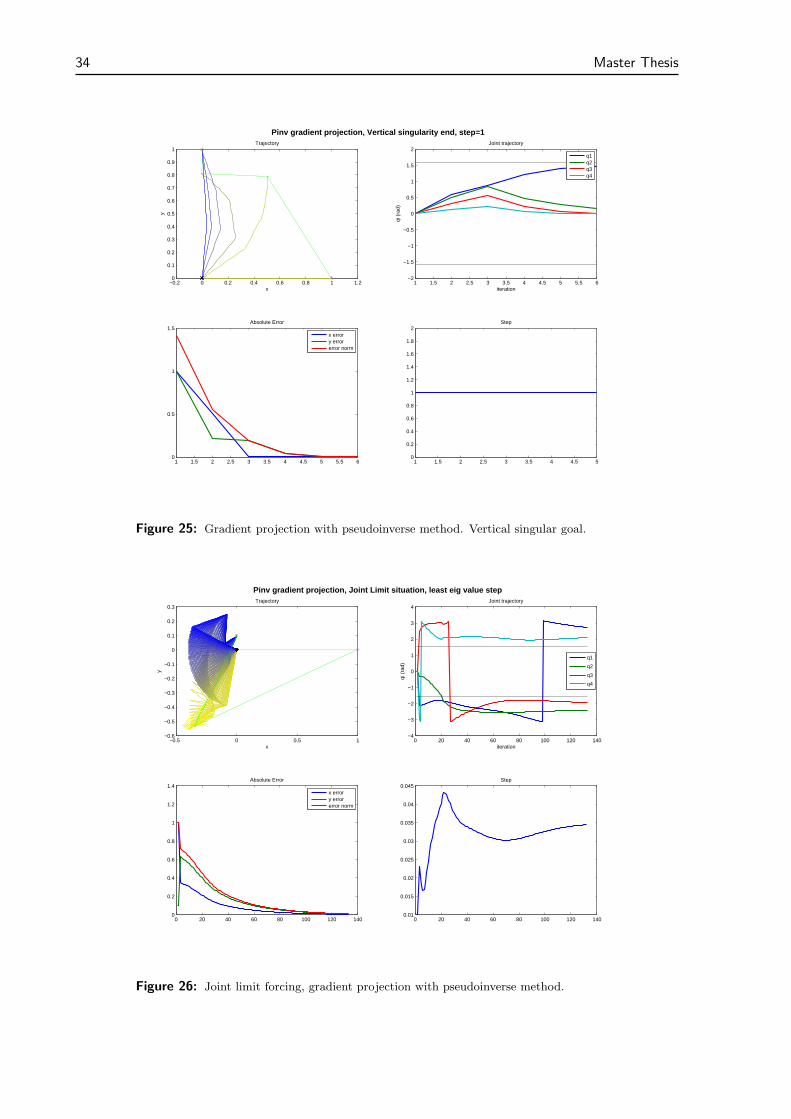
• Vertical singular end position using M .Computation time of 0.0914s.As we can see in Figure 25, the method converges fastly aswithout the kernel projection (Figure 14).
• Joint limit forcing. With a computation time of 0.3307s, we now show the effect of project-ing the gradient of the H function (Figure 26) which, theorically, pushes the joints awayfrom their limits. We can see that, even with a small step, the fact that the joint limitsare only treated on the kernel of the main task is not enough to ensure those are avoided.
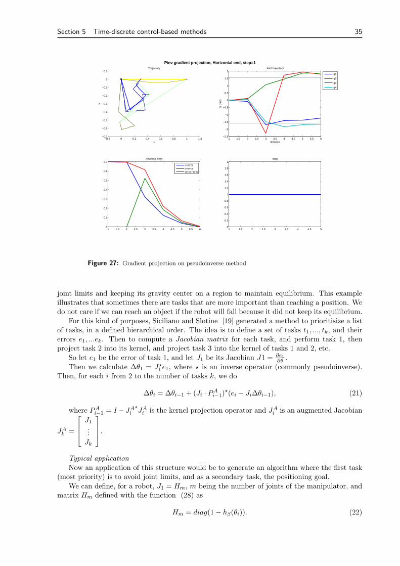
• Horizontal end position. we can now see in Figure 27 (with a computation time of 0.1021s)that the gradient of the manipulability (∇M) has overcome the problem of getting stuckin the initial singularity.
5.3.6 Task priority
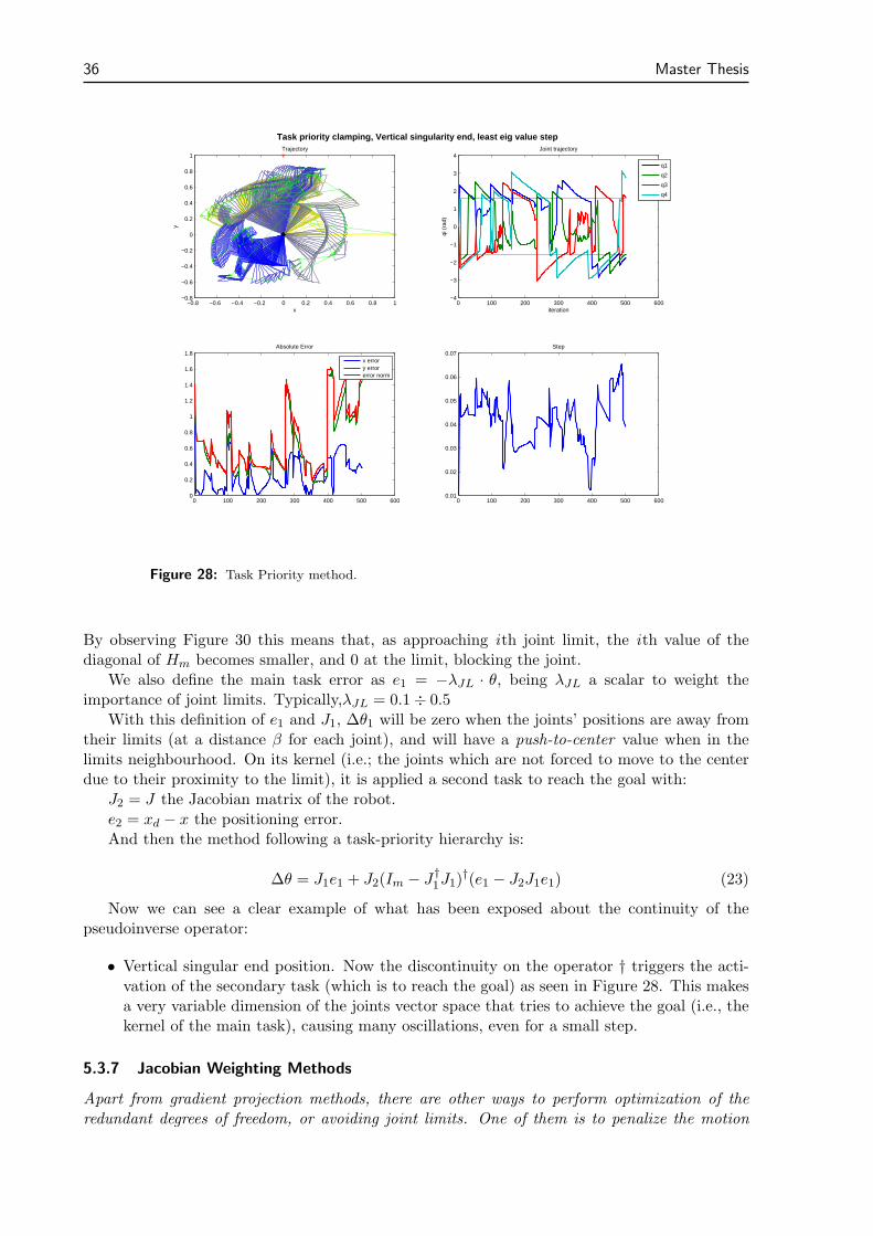
Task priority algorithms are a generalization of the gradient projection methods. The main ideais to have an ordered set of tasks, and project each task onto the kernel of the previous tasks
When dealing with redundant degrees of freedom, sometimes we have many tasks to perform.One example would be a humanoid robot trying to reach an object with its hand, respecting its
34 Master Thesis
−0.2 0 0.2 0.4 0.6 0.8 1 1.20
0.1
0.2
0.3
0.4
0.5
0.6
0.7
0.8
0.9
1
x
y
Trajectory
1 1.5 2 2.5 3 3.5 4 4.5 5 5.5 6−2
−1.5
−1
−0.5
0
0.5
1
1.5
2
iteration
qi (
rad)
Joint trajectory
q1q2q3q4
1 1.5 2 2.5 3 3.5 4 4.5 5 5.5 60
0.5
1
1.5Absolute Error
x errory errorerror norm
Pinv gradient projection, Vertical singularity end, step=1
1 1.5 2 2.5 3 3.5 4 4.5 50
0.2
0.4
0.6
0.8
1
1.2
1.4
1.6
1.8
2Step
Figure 25: Gradient projection with pseudoinverse method. Vertical singular goal.
−0.5 0 0.5 1−0.6
−0.5
−0.4
−0.3
−0.2
−0.1
0
0.1
0.2
0.3
x
y
Trajectory
0 20 40 60 80 100 120 140−4
−3
−2
−1
0
1
2
3
4
iteration
qi (
rad)
Joint trajectory
q1
q2
q3
q4
0 20 40 60 80 100 120 1400
0.2
0.4
0.6
0.8
1
1.2
1.4Absolute Error
x errory errorerror norm
Pinv gradient projection, Joint Limit situation, least eig value step
0 20 40 60 80 100 120 1400.01
0.015
0.02
0.025
0.03
0.035
0.04
0.045Step
Figure 26: Joint limit forcing, gradient projection with pseudoinverse method.
Section 5 Time-discrete control-based methods 35
−0.2 0 0.2 0.4 0.6 0.8 1 1.2−0.7
−0.6
−0.5
−0.4
−0.3
−0.2
−0.1
0
0.1Trajectory
x
y
1 1.5 2 2.5 3 3.5 4 4.5 5 5.5 6−2.5
−2
−1.5
−1
−0.5
0
0.5
1
1.5
2
iteration
qi (
rad)
Joint trajectory
q1
q2
q3
q4
1 1.5 2 2.5 3 3.5 4 4.5 5 5.5 60
0.1
0.2
0.3
0.4
0.5
0.6
0.7Absolute Error
x errory errorerror norm
Pinv gradient projection, Horizontal end, step=1
1 1.5 2 2.5 3 3.5 4 4.5 50
0.2
0.4
0.6
0.8
1
1.2
1.4
1.6
1.8
2Step
Figure 27: Gradient projection on pseudoinverse method
joint limits and keeping its gravity center on a region to maintain equilibrium. This exampleillustrates that sometimes there are tasks that are more important than reaching a position. Wedo not care if we can reach an object if the robot will fall because it did not keep its equilibrium.
For this kind of purposes, Siciliano and Slotine [19] generated a method to prioritisize a listof tasks, in a defined hierarchical order. The idea is to define a set of tasks t1, ..., tk, and theirerrors e1, ...ek. Then to compute a Jacobian matrix for each task, and perform task 1, thenproject task 2 into its kernel, and project task 3 into the kernel of tasks 1 and 2, etc.
So let e1 be the error of task 1, and let J1 be its Jacobian J1 = ∂e1∂θ .
Then we calculate ∆θ1 = J⋆1 e1, where ⋆ is an inverse operator (commonly pseudoinverse).
Then, for each i from 2 to the number of tasks k, we do
∆θi = ∆θi−1 + (Ji · PAi−1)
⋆(ei − Ji∆θi−1), (21)
where PAi−1 = I−JA
i⋆JAi is the kernel projection operator and JA
i is an augmented Jacobian
JAk =
J1...Jk
.
Typical application
Now an application of this structure would be to generate an algorithm where the first task(most priority) is to avoid joint limits, and as a secondary task, the positioning goal.
We can define, for a robot, J1 = Hm, m being the number of joints of the manipulator, andmatrix Hm defined with the function (28) as
Hm = diag(1− hβ(θi)). (22)
36 Master Thesis
−0.8 −0.6 −0.4 −0.2 0 0.2 0.4 0.6 0.8 1−0.8
−0.6
−0.4
−0.2
0
0.2
0.4
0.6
0.8
1
x
y
Trajectory
0 100 200 300 400 500 600−4
−3
−2
−1
0
1
2
3
4
iteration
qi (
rad)
Joint trajectory
q1
q2
q3
q4
0 100 200 300 400 500 6000
0.2
0.4
0.6
0.8
1
1.2
1.4
1.6
1.8Absolute Error
x errory errorerror norm
Task priority clamping, Vertical singularity end, least eig value step
0 100 200 300 400 500 6000.01
0.02
0.03
0.04
0.05
0.06
0.07Step
Figure 28: Task Priority method.
By observing Figure 30 this means that, as approaching ith joint limit, the ith value of thediagonal of Hm becomes smaller, and 0 at the limit, blocking the joint.
We also define the main task error as e1 = −λJL · θ, being λJL a scalar to weight theimportance of joint limits. Typically,λJL = 0.1÷ 0.5
With this definition of e1 and J1, ∆θ1 will be zero when the joints’ positions are away fromtheir limits (at a distance β for each joint), and will have a push-to-center value when in thelimits neighbourhood. On its kernel (i.e.; the joints which are not forced to move to the centerdue to their proximity to the limit), it is applied a second task to reach the goal with:
J2 = J the Jacobian matrix of the robot.e2 = xd − x the positioning error.And then the method following a task-priority hierarchy is:
∆θ = J1e1 + J2(Im − J†1J1)
†(e1 − J2J1e1) (23)
Now we can see a clear example of what has been exposed about the continuity of thepseudoinverse operator:
• Vertical singular end position. Now the discontinuity on the operator † triggers the acti-vation of the secondary task (which is to reach the goal) as seen in Figure 28. This makesa very variable dimension of the joints vector space that tries to achieve the goal (i.e., thekernel of the main task), causing many oscillations, even for a small step.
5.3.7 Jacobian Weighting Methods
Apart from gradient projection methods, there are other ways to perform optimization of theredundant degrees of freedom, or avoiding joint limits. One of them is to penalize the motion
Section 5 Time-discrete control-based methods 37
of some of the joints, depending on a weighting matrix. This weighting matrix will modify eachjoint’s response according to a specified criterion.
In [3], Chan and Dubey define the ∆θ which minimizes
‖θ‖W =√θTWθ, (24)
where W is an m × m diagonal matrix reflecting a weight on each joint, depending on itsrelevance (according to a specified criteria) instead of the common euclidean norm ‖θ‖ =
√θT θ.
To this purpose, a new set of joints can be defined as
θW = W 1/2θ, (25)
then
x = Jθ = JW−1/2W 1/2θ = JW−1/2θW = JW θW (26)
and we can compute the pseudoinverse of JW
J†W = JT
W (JWJTW )−1 = W−1/2JT (JW−1/2W−1/2JT )−1 = W−1/2JT (JW−1JT )−1
And if θW = J†W x, we have θ = W−1JT (JW−1JT )−1x.
This pseudoinverse matrix of JW can also be damped or filtered, but then always premulti-plied by W−1/2, which comes from the change of θW to a joint change on θ.
The influence of ωi = Wi,i is that, the greater the ωi, the less θi will vary in the step.
With this structure created, one can take W = diag(ω1, ...ωm), where ωi = 1 + |∂H∂θi |, beingH : Q ⊆ Rm → R a scalar value to minimize. A typical choice of H is like in eq. (6). Whattranslates into:
∂H∂θi
=(θmax
i −θmini )2(2θi−θuimax−θmin
i )
2m(θmaxi −θi)2(θi−θmin
i )2
Nevertheless, in [3] it is pointed out that this gradient does not give information aboutwhether a joint is moving towards its limit or away from it, so it might be reducing a movementthat, not only is valid, but also sends the joint to a more central position. To this purpose,in [3] it is defined, for two consecutive steps k and k+1 ∆HiK = |∂H∂θi |k − |∂H∂θi |k−1 and redefine
ωiK =
{
1 + |∂H∂θi | if ∆HiK ≥ 0
1 if ∆HiK < 0
With this new weight, if the robot is moving towards a joint limit, the joint is weighted toreduce its influence and so, avoid it. And it moves away from a joint limit, the joint is notaffected by a weight.
To perform some examples, the case of a vertical singular end position presents no prob-lems, while the horizontal end position does have the problem as in the Jacobian transposed orpseudoinverse methods. Now when forcing a limit:
• Joint limit forcing. Figure 29 (computation time of 0.0622s) we can see the behaviour isbetter than with the gradient projection method, and it does push joints back to theirrange, although it does not achieve such task 100% efficiently.
5.3.8 Joint Clamping
An intuitive way of avoiding to surpass a joint limit, is to block the value of the joint trying tosurpass its limit. We call this clamping a joint.
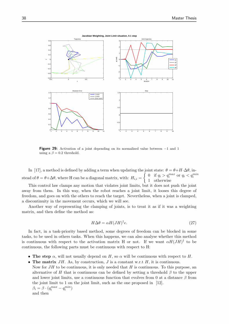
38 Master Thesis
−0.5 0 0.5 1−0.8
−0.6
−0.4
−0.2
0
0.2
0.4
0.6
0.8
x
y
Trajectory
1 2 3 4 5 6 7 8 9 10 11−3
−2
−1
0
1
2
3
iteration
qi (
rad)
Joint trajectory
q1
q2
q3
q4
1 2 3 4 5 6 7 8 9 10 110
0.2
0.4
0.6
0.8
1
1.2
1.4Absolute Error
x errory errorerror norm
Jacobian Weighting, Joint Limit situation, 0.1 step
1 2 3 4 5 6 7 8 9 10−1
−0.5
0
0.5
1
1.5Step
Figure 29: Activation of a joint depending on its normalised value between −1 and 1using a β = 0.2 threshold.
In [17], a method is defined by adding a term when updating the joint state: θ = θ+H ·∆θ, in-
stead of θ = θ+∆θ, where H can be a diagonal matrix, with: Hi,i =
{
0 if qi > qmaxi or qi < qmin
i
1 otherwiseThis control law clamps any motion that violates joint limits, but it does not push the joint
away from them. In this way, when the robot reaches a joint limit, it looses this degree offreedom, and goes on with the others to reach the target. Nevertheless, when a joint is clamped,a discontinuity in the movement occurs, which we will see.
Another way of representing the clamping of joints, is to treat it as if it was a weightingmatrix, and then define the method as:
H∆θ = αH(JH)†e. (27)
In fact, in a task-priority based method, some degrees of freedom can be blocked in sometasks, to be used in others tasks. When this happens, we can also analyse whether this methodis continuous with respect to the activation matrix H or not. If we want αH(JH)† to becontinuous, the following parts must be continuous with respect to H:
• The step α, will not usually depend on H, so α will be continuous with respect to H.
• The matrix JH. As, by construction, J is a constant w.r.t H, it is continuous.Now for JH to be continuous, it is only needed that H is continuous. To this purpose, analternative of H that is continuous can be defined by setting a threshold β to the upperand lower joint limits, use a continuous function that evolves from 0 at a distance β fromthe joint limit to 1 on the joint limit, such as the one proposed in [12].βi = β · (qmax
i − qmini )
and then
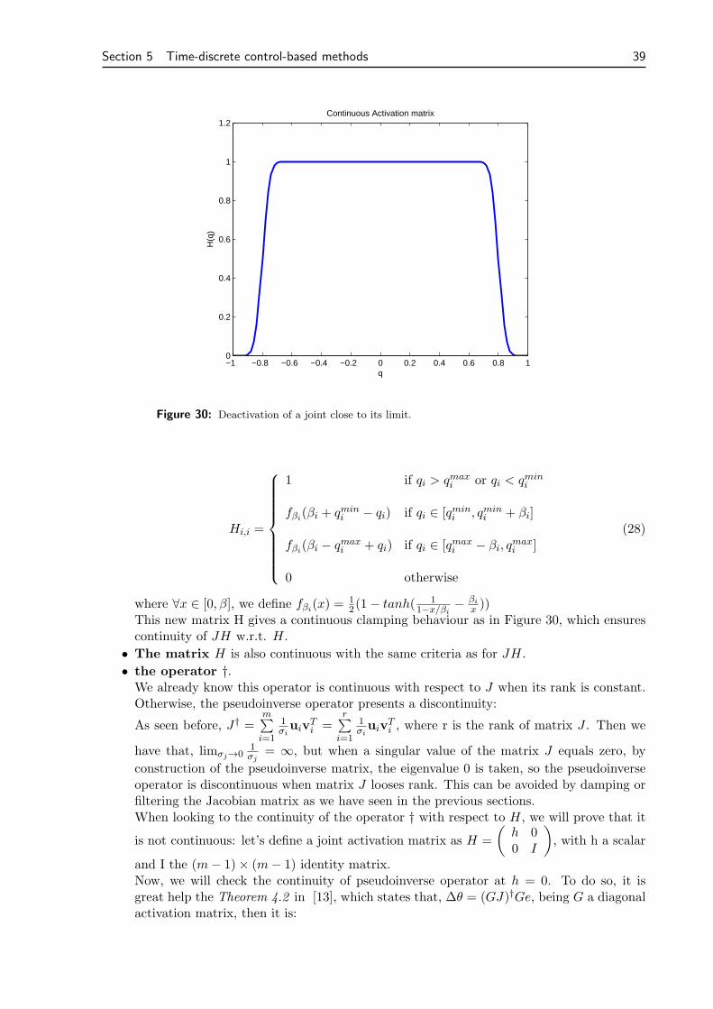
Section 5 Time-discrete control-based methods 39
−1 −0.8 −0.6 −0.4 −0.2 0 0.2 0.4 0.6 0.8 10
0.2
0.4
0.6
0.8
1
1.2
q
H(q
)
Continuous Activation matrix
Figure 30: Deactivation of a joint close to its limit.
Hi,i =
1 if qi > qmaxi or qi < qmin
i
fβi(βi + qmin
i − qi) if qi ∈ [qmini , qmin
i + βi]
fβi(βi − qmax
i + qi) if qi ∈ [qmaxi − βi, q
maxi ]
0 otherwise
(28)
where ∀x ∈ [0, β], we define fβi(x) = 1
2(1− tanh( 11−x/βi
− βi
x ))This new matrix H gives a continuous clamping behaviour as in Figure 30, which ensurescontinuity of JH w.r.t. H.
• The matrix H is also continuous with the same criteria as for JH.
• the operator †.We already know this operator is continuous with respect to J when its rank is constant.Otherwise, the pseudoinverse operator presents a discontinuity:
As seen before, J† =m∑
i=1
1σiuiv
Ti =
r∑
i=1
1σiuiv
Ti , where r is the rank of matrix J . Then we
have that, limσj→01σj
= ∞, but when a singular value of the matrix J equals zero, by
construction of the pseudoinverse matrix, the eigenvalue 0 is taken, so the pseudoinverseoperator is discontinuous when matrix J looses rank. This can be avoided by damping orfiltering the Jacobian matrix as we have seen in the previous sections.When looking to the continuity of the operator † with respect to H, we will prove that it
is not continuous: let’s define a joint activation matrix as H =
(
h 00 I
)
, with h a scalar
and I the (m− 1)× (m− 1) identity matrix.Now, we will check the continuity of pseudoinverse operator at h = 0. To do so, it isgreat help the Theorem 4.2 in [13], which states that, ∆θ = (GJ)†Ge, being G a diagonalactivation matrix, then it is:
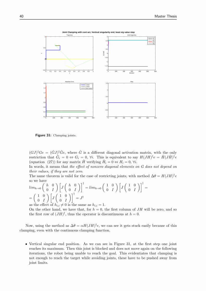
40 Master Thesis
0 0.1 0.2 0.3 0.4 0.5 0.6 0.7 0.8 0.9 1−0.5
0
0.5
1
x
y
Trajectory
0 100 200 300 400 500 600−2
−1.5
−1
−0.5
0
0.5
1
1.5
2
iteration
qi (
rad)
Joint trajectory
q1q2q3q4
0 100 200 300 400 500 6000.2
0.4
0.6
0.8
1
1.2
1.4
1.6Absolute Error
x errory errorerror norm
Joint Clamping with cont act, Vertical singularity end, least eig value step
0 100 200 300 400 500 600−1
−0.5
0
0.5
1
1.5Step
Figure 31: Clamping joints.
(GJ)†Ge = (GJ)†Ge, where G is a different diagonal activation matrix, with the onlyrestriction that Gi = 0 ⇔ Gi = 0, ∀i. This is equivalent to say H(JH)†e = H(JH)†e(equation (27)) for any matrix H verifying Hi = 0 ⇔ Hi = 0, ∀i.In words, it means that the effect of nonzero diagonal elements on G does not depend ontheir values, if they are not zero.The same theorem is valid for the case of restricting joints, with method ∆θ = H(JH)†eso we have
limh→0
(
h 00 I
)[
J
(
h 00 I
)]†
= limh→0
(
1 00 I
)[
J
(
1 00 I
)]†
=
=
(
1 00 I
)[
J
(
1 00 I
)]†
= J†
as the effect of hi,i 6= 0 is the same as hi,i = 1.On the other hand, we have that, for h = 0, the first column of JH will be zero, and sothe first row of (JH)†, thus the operator is discontinuous at h = 0.
Now, using the method as ∆θ = αH(JH)†e, we can see it gets stuck easily because of thisclamping, even with the continuous clamping function.
• Vertical singular end position. As we can see in Figure 31, at the first step one jointreaches its maximum. Then this joint is blocked and does not move again on the followingiterations, the robot being unable to reach the goal. This evidentiates that clamping isnot enough to reach the target while avoiding joints, these have to be pushed away fromjoint limits.
Section 5 Time-discrete control-based methods 41
5.3.9 Continuous Clamping
To solve the discontinuity on the activation/deactivation of joints, a new inverse operator hasbeen created to assure the continuity of the method when the activation of tasks or joint istriggered. These inverse operator will be defined so as to take the value of the Moore-Penrosepseudoinverse when joints are fully active or blocked, and with this inverse operators a continuoustask-priority method can be used. For practical reasons, we recommend reading [12] to betterunderstand the definition of this inverse
As we have seen, the pseudoinverse operator is not continuous when dealing with activationmatrices or task priority. To this purpose, as introduced, [14] and [13] propose a continuousw.r.t activation matrices inverse, based on a diagonal activation matrix to clamp tasks, and alsojoints on an algorithm.
• Task Clamping. The original purpose of [14] and [13] is to create a control scheme inwhich tasks may vary its activation, named varying-feature-set tasks, which are tasks withthe form eq = Ge, G being a diagonal continuous matrix with its values in the interval[0, 1]. When gi = Gi,i = 1, the task is active. On the other hand, when gi = Gi,i = 0, taski becomes inactive.An example for this would be, in an oriented spatial robot (where the task space has 6degrees of freedom, 3 for position and 3 for orientation), to activate the orientation trackingon the Jacobian matrix of a manipulatori only when the robot is close enough to the goal.Then, matrix G would be:
G =
(
I3 03×3
03×3 A
)
, where
A =
03×3 if e > emin − ǫf(e, emin, ǫ) · I3 if emin > e > emin − ǫI3 if e < emin
,
being f(e, emin, ǫ) a smooth function as in equation (28).
To this purpose, a control method as ∆θ = (GJ)†Ge could be used, but it would havethe continuity problem as previously commented. To solve it, a new inverse operator isdefined in these articles, as
⊕ : Mn×m(R)×Mn×n(R) → Mm×n(R)(A,G) 7→ A⊕G
to verify:- Given a matrix A, ⊕ is continuous with respect to G.That is to avoid the discontinuities caused by the change of task activation on matrix G.- if ∀i = 1..n, gi ∈ {0, 1}, then A⊕G = (GA)† = (GA)†GThis means that when matrix G is a binary diagonal matrix, the operator must have thesame values as the Moore-Penrose pseudoinverse. This is to keep consistence with thestandard pseudoinverse.
With these specifications, a set of auxiliar matrices are defined: The Coupling Matricesof a Matrix J are n ×m matrices indexed by the elements of the power set ℘ (the set ofsubsets) of N = {1, ..., n}if P = ∅, X∅ = 0m×n
else ∀P ∈ ℘(N), XP = J†P −
∑
Q(P
XQ
42 Master Thesis
where JP = G0J , being G0 a binary diagonal matrix with G0i = 1 if i ∈ P and 0 otherwise.
With these coupling matrices, the Continuous Inverse of a Matrix J with task activationgiven by G is defined as:
J⊕G =∑
P∈℘(N)
(∏
i∈P
gi)XP =∑
P∈℘(N)
(∏
i∈P
gi)(∏
i/∈P
(1− gi))J†P (29)
And it is proven, again in [14], that this pseudoinverse operator verifies the two propertiesrequired.
Also, in [12] this pseudoinverse is generalised for the case of a non-diagonal activationmatrix, say W. If we use the singular value decomposition of W, then W = USUT and(WJ)†W = (SUTJ)†SUT , and the Continuous Inverse if a Matrix J with task activationgiven by a non-diagonal matrix W is
J⊕W = J⊕SU UT =
∑
P∈℘(N)
(
∏
i∈P
σi
)
XJUP UT , (30)
where XJUP are the task-coupling matrices of JU = UTJ .
• Joint Clamping. As seen before, what we expect to do is to restrict a joint movementto avoid its limits in spite of a task. To this purpose, our starting control scheme wouldhave the form∆θ = H(JH)†e, but defining an operator
⊕ : Mn×m(R)×Mm×m(R) → Mm×n(R)(A,H) 7→ AH⊕
we can calculate the adapted Continuous Inverse of a Matrix J with joint activation givenby H as:
JH⊕ =∑
Q∈℘(M)
(∏
i∈Q
hi)YQ =∑
Q∈℘(M)
(∏
i∈Q
hi)(∏
i/∈Q
(1− hi))J†Q (31)
With its coupling matrices now defined asif Q = ∅, X∅ = 0mxn
else ∀Q ∈ ℘(M), YQ = J†Q − ∑
R(Q
YR
where JQ = JH0, beingH0 a binary diagonal matrix withH0i = 1 if i ∈ Q and 0 otherwise.
This matrix is also defined in [12] as a left-activated continuous inverse from the task-clamping continuous inverse:JH⊕ = ((JT )⊕H)T
Note that, then it is ((JT )⊕H)T =∑
Q∈℘(M)
(∏
i∈Q
hi)(∏
i/∈Q
(1 − hi))YQ (i.e.: both definitions
match)ProofBy definition, we have that ((JT )⊕H)T =
∑
P∈℘(N)
(∏
i∈P
gi)(∏
i/∈P
(1 − gi))XTP , being XP the
taks activation matrices of JT .
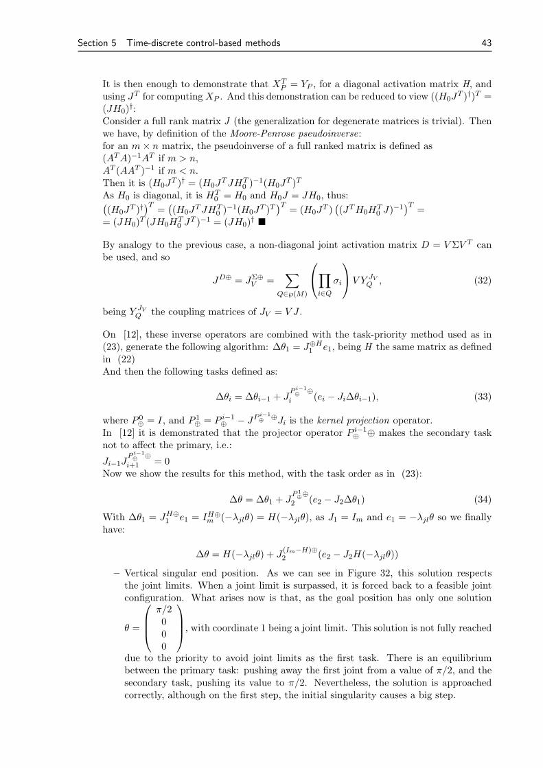
Section 5 Time-discrete control-based methods 43
It is then enough to demonstrate that XTP = YP , for a diagonal activation matrix H, and
using JT for computingXP . And this demonstration can be reduced to view ((H0JT )†)T =
(JH0)†:
Consider a full rank matrix J (the generalization for degenerate matrices is trivial). Thenwe have, by definition of the Moore-Penrose pseudoinverse:for an m× n matrix, the pseudoinverse of a full ranked matrix is defined as(ATA)−1AT if m > n,AT (AAT )−1 if m < n.Then it is (H0J
T )† = (H0JTJHT
0 )−1(H0J
T )T
As H0 is diagonal, it is HT0 = H0 and H0J = JH0, thus:
(
(H0JT )†)T
=(
(H0JTJHT
0 )−1(H0J
T )T)T
= (H0JT )(
(JTH0HT0 J)
−1)T
== (JH0)
T (JH0HT0 J
T )−1 = (JH0)†�
By analogy to the previous case, a non-diagonal joint activation matrix D = V ΣV T canbe used, and so
JD⊕ = JΣ⊕V =
∑
Q∈℘(M)
∏
i∈Q
σi
V Y JVQ , (32)
being Y JVQ the coupling matrices of JV = V J .
On [12], these inverse operators are combined with the task-priority method used as in(23), generate the following algorithm: ∆θ1 = J⊕H
1 e1, being H the same matrix as definedin (22)And then the following tasks defined as:
∆θi = ∆θi−1 + JP i−1
⊕⊕
i (ei − Ji∆θi−1), (33)
where P 0⊕ = I, and P 1
⊕ = P i−1⊕ − JP i−1
⊕⊕Ji is the kernel projection operator.
In [12] it is demonstrated that the projector operator P i−1⊕ ⊕ makes the secondary task
not to affect the primary, i.e.:
Ji−1JP i−1
⊕⊕
i+1 = 0Now we show the results for this method, with the task order as in (23):
∆θ = ∆θ1 + JP 1
⊕⊕
2 (e2 − J2∆θ1) (34)
With ∆θ1 = JH⊕1 e1 = IH⊕
m (−λjlθ) = H(−λjlθ), as J1 = Im and e1 = −λjlθ so we finallyhave:
∆θ = H(−λjlθ) + J(Im−H)⊕2 (e2 − J2H(−λjlθ))
– Vertical singular end position. As we can see in Figure 32, this solution respectsthe joint limits. When a joint limit is surpassed, it is forced back to a feasible jointconfiguration. What arises now is that, as the goal position has only one solution
θ =
π/2000
, with coordinate 1 being a joint limit. This solution is not fully reached
due to the priority to avoid joint limits as the first task. There is an equilibriumbetween the primary task: pushing away the first joint from a value of π/2, and thesecondary task, pushing its value to π/2. Nevertheless, the solution is approachedcorrectly, although on the first step, the initial singularity causes a big step.
44 Master Thesis
−0.4 −0.2 0 0.2 0.4 0.6 0.8 10
0.1
0.2
0.3
0.4
0.5
0.6
0.7
0.8
0.9
1
x
y
Trajectory
0 100 200 300 400 500 600−3
−2
−1
0
1
2
3
iteration
qi (
rad)
Joint trajectory
q1
q2
q3
q4
0 100 200 300 400 500 6000
0.5
1
1.5Absolute Error
x errory errorerror norm
Task priority clamping with cont activation, Vertical singularity end, 0.1 step
0 100 200 300 400 500 600−1
−0.5
0
0.5
1
1.5Step
Figure 32: Continuous clamping task priority algorithm.
– Horizontal end position. For this case, as could be expected, the robot won’t move.This is because it has been assured a continuity depending on the activation matrix,but no filtering or similar has been applied to solve singularities.
– Joint limit forcing. Now we could expect a correct behaviour of the robot when tryingto force its limits. In spite of this, what we find is in Figure 33. This is due to the factthat the solution to this desired goal does not exist, so the algorithm keeps lookingfor an equilibrium point, that can only be an algorithmic singularity.
5.4 Proposed methods
Apart from what we have been exposing, now we propose two new methods. The first one,is a new way of filtering the Jacobian matrix, so as to effectively avoid large gains and largecondition numbers of the Jacobian matrix, while the second one is a mixture of the continuoustask-priority clamping algorithm with the selective damping, to find a very smooth algorithm,as we will see.
5.4.1 Smooth eigenvalue filtering.
Although it may seem that the Jacobian damping and filtering would solve any problem whena singularity occurs, if we analise the behaviour of the function
fλ : R → R
σ 7→ fλ(σ) =σ
σ2+λ2
we can see that its derivative w.r.t σ is∂fλ∂σ = λ2−σ2
(σ2+λ2)2= 0 ⇔ σ = ±λ
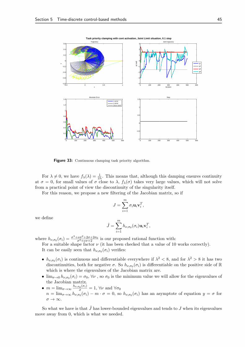
Section 5 Time-discrete control-based methods 45
−0.5 0 0.5 1−0.8
−0.6
−0.4
−0.2
0
0.2
0.4
0.6
x
y
Trajectory
0 100 200 300 400 500 600−4
−3
−2
−1
0
1
2
3
iteration
qi (
rad)
Joint trajectory
q1
q2
q3
q4
0 100 200 300 400 500 6000
0.2
0.4
0.6
0.8
1
1.2
1.4Absolute Error
x errory errorerror norm
Task priority clamping with cont activation, Joint Limit situation, 0.1 step
0 100 200 300 400 500 600−1
−0.5
0
0.5
1
1.5Step
Figure 33: Continuous clamping task priority algorithm.
For λ 6= 0, we have fλ(λ) =12λ . This means that, although this damping ensures continuity
at σ = 0, for small values of σ close to λ, fλ(σ) takes very large values, which will not solvefrom a practical point of view the discontinuity of the singularity itself.
For this reason, we propose a new filtering of the Jacobian matrix, so if
J =m∑
i=1
σiuivTi ,
we define
J =m∑
i=1
hν,σ0(σi)uiv
Ti ,
where hν,σ0(σi) =
σ3+νσ2+2σ+2σ0
σ2+νσ+2is our proposed rational function with:
For a suitable shape factor ν (it has been checked that a value of 10 works correctly).It can be easily seen that hν,σ0
(σi) verifies:
• hν,σ0(σi) is continuous and differentiable everywhere if λ2 < 8, and for λ2 > 8 it has two
discontinuities, both for negative σ. So hν,σ0(σi) is differentiable on the positive side of R
which is where the eigenvalues of the Jacobian matrix are.
• limσ→0 hν,σ0(σi) = σ0, ∀ν , so σ0 is the minimum value we will allow for the eigenvalues of
the Jacobian matrix.
• m = limσ→∞hν,σ0
(σi)σ = 1, ∀ν and ∀σ0
n = limσ→∞ hν,σ0(σi) − m · σ = 0, so hν,σ0
(σi) has an asymptote of equation y = σ forσ → ∞.
So what we have is that J has lower-bounded eigenvalues and tends to J when its eigenvaluesmove away from 0, which is what we needed.
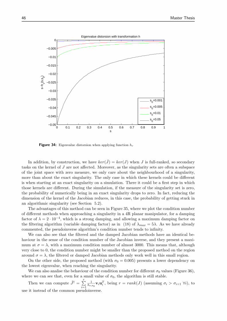
46 Master Thesis
0 0.1 0.2 0.3 0.4 0.5 0.6 0.7 0.8 0.9 1−0.05
−0.045
−0.04
−0.035
−0.03
−0.025
−0.02
−0.015
−0.01
−0.005
0
s
s−h v(s
,s0)
Eigenvalue distorsion with transformation h
s0=0.001
s0=0.005
s0=0.01
s0=0.05
Figure 34: Eigenvalue distorsion when applying function hν
In addition, by construction, we have ker(J) = ker(J) when J is full-ranked, so secondarytasks on the kernel of J are not affected. Moreover, as the singularity sets are often a subspaceof the joint space with zero measure, we only care about the neighbourhood of a singularity,more than about the exact singularity. The only case in which these kernels could be differentis when starting at an exact singularity on a simulation. There it could be a first step in whichthose kernels are different. During the simulation, if the measure of the singularity set is zero,the probability of numerically being in an exact singularity drops to zero. In fact, reducing thedimension of the kernel of the Jacobian reduces, in this case, the probability of getting stuck inan algorithmic singularity (see Section 5.2).
The advantages of this method can be seen in Figure 35, where we plot the condition numberof different methods when approaching a singularity in a 4R planar manipulator, for a dampingfactor of λ = 2 · 10−4, which is a strong damping, and allowing a maximum damping factor onthe filtering algorithm (variable damping factor) as in (18) of λmax = 5λ. As we have alreadycommented, the pseudoinverse algorithm’s condition number tends to infinity.
We can also see that the filtered and the damped Jacobian methods have an identical be-haviour in the sense of the condition number of the Jacobian inverse, and they present a maxi-mum at σ = λ, with a maximum condition number of almost 3000. This means that, althoughvery close to 0, the condition number might be smaller than the proposed method on the regionaround σ = λ, the filtered or damped Jacobian methods only work well in this small region.
On the other side, the proposed method (with σ0 = 0.005) presents a lower dependency onthe lowest eigenvalue, when reaching the singularity.
We can also analise the behaviour of the condition number for different σ0 values (Figure 36),where we can see that, even for a small value of σ0, the algorithm is still stable.
Then we can compute J† =r∑
i=1
1hν,σ0
viuTi , being r = rank(J) (assuming σi > σi+1 ∀i), to
use it instead of the common pseudoinverse.
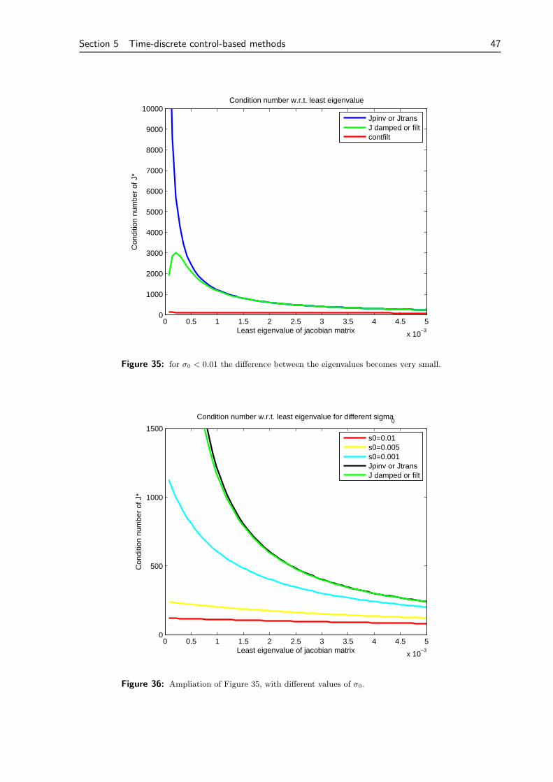
Section 5 Time-discrete control-based methods 47
0 0.5 1 1.5 2 2.5 3 3.5 4 4.5 5
x 10−3
0
1000
2000
3000
4000
5000
6000
7000
8000
9000
10000
Least eigenvalue of jacobian matrix
Con
ditio
n nu
mbe
r of
J*
Condition number w.r.t. least eigenvalue
Jpinv or JtransJ damped or filtcontfilt
Figure 35: for σ0 < 0.01 the difference between the eigenvalues becomes very small.
0 0.5 1 1.5 2 2.5 3 3.5 4 4.5 5
x 10−3
0
500
1000
1500
Least eigenvalue of jacobian matrix
Con
ditio
n nu
mbe
r of
J*
Condition number w.r.t. least eigenvalue for different sigma0
s0=0.01s0=0.005s0=0.001Jpinv or JtransJ damped or filt
Figure 36: Ampliation of Figure 35, with different values of σ0.
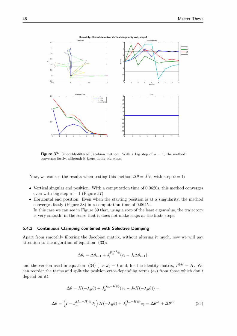
48 Master Thesis
−0.5 0 0.5 1−0.2
0
0.2
0.4
0.6
0.8
1
1.2
x
y
Trajectory
1 2 3 4 5 6 7 8 9−3
−2
−1
0
1
2
3
iteration
qi (
rad)
Joint trajectory
q1
q2
q3
q4
1 2 3 4 5 6 7 8 90
0.5
1
1.5Absolute Error
x errory errorerror norm
Smoothly−filtered Jacobian, Vertical singularity end, step=1
1 2 3 4 5 6 7 80
0.2
0.4
0.6
0.8
1
1.2
1.4
1.6
1.8
2Step
Figure 37: Smoothly-filtered Jacobian method. With a big step of α = 1, the methodconverges fastly, although it keeps doing big steps.
Now, we can see the results when testing this method ∆θ = J†e, with step α = 1:
• Vertical singular end position. With a computation time of 0.0620s, this method convergeseven with big step α = 1 (Figure 37)
• Horizontal end position. Even when the starting position is at a singularity, the methodconverges fastly (Figure 38) in a computation time of 0.0645s.In this case we can see in Figure 39 that, using a step of the least eigenvalue, the trajectoryis very smooth, in the sense that it does not make leaps at the firsts steps.
5.4.2 Continuous Clamping combined with Selective Damping
Apart from smoothly filtering the Jacobian matrix, without altering it much, now we will payattention to the algorithm of equation (33):
∆θi = ∆θi−1 + JP i−1
⊕⊕
i (ei − Ji∆θi−1),
and the version used in equation (34) ( as J1 = I and, for the identity matrix, I⊕H = H. Wecan reorder the terms and split the position error-depending terms (e2) from those which don’tdepend on it):
∆θ = H(−λjlθ) + J(Im−H)⊕2 (e2 − J2H(−λjlθ)) =
∆θ =(
I − J(Im−H)⊕2 J2
)
H(−λjlθ) + J(Im−H)⊕2 e2 = ∆θ∗1 +∆θ∗2 (35)
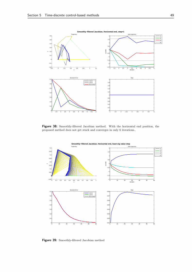
Section 5 Time-discrete control-based methods 49
−0.2 0 0.2 0.4 0.6 0.8 1 1.2−0.2
−0.1
0
0.1
0.2
0.3
0.4
0.5
0.6Trajectory
x
y
1 1.5 2 2.5 3 3.5 4 4.5 5 5.5 6−2.5
−2
−1.5
−1
−0.5
0
0.5
1
1.5
2
iteration
qi (
rad)
Joint trajectory
q1
q2
q3
q4
1 1.5 2 2.5 3 3.5 4 4.5 5 5.5 60
0.1
0.2
0.3
0.4
0.5
0.6
0.7Absolute Error
x errory errorerror norm
Smoothly−filtered Jacobian, Horizontal end, step=1
1 1.5 2 2.5 3 3.5 4 4.5 50
0.2
0.4
0.6
0.8
1
1.2
1.4
1.6
1.8
2Step
Figure 38: Smoothly-filtered Jacobian method. With the horizontal end position, theproposed method does not get stuck and converges in only 6 iterations..
0 0.1 0.2 0.3 0.4 0.5 0.6 0.7 0.8 0.9 1−0.05
0
0.05
0.1
0.15
0.2
0.25
0.3
0.35
0.4Trajectory
x
y
0 10 20 30 40 50 60−2
−1.5
−1
−0.5
0
0.5
1
1.5
2
iteration
qi (
rad)
Joint trajectory
q1
q2
q3
q4
0 10 20 30 40 50 600
0.1
0.2
0.3
0.4
0.5
0.6
0.7Absolute Error
x errory errorerror norm
Smoothly−filtered Jacobian, Horizontal end, least eig value step
0 10 20 30 40 50 600.01
0.02
0.03
0.04
0.05
0.06
0.07
0.08Step
Figure 39: Smoothly-filtered Jacobian method
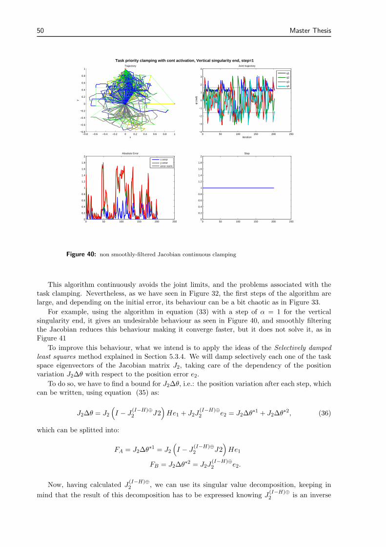
50 Master Thesis
−0.8 −0.6 −0.4 −0.2 0 0.2 0.4 0.6 0.8 1−0.8
−0.6
−0.4
−0.2
0
0.2
0.4
0.6
0.8
1Trajectory
x
y
0 50 100 150 200 250−4
−3
−2
−1
0
1
2
3
4
iteration
qi (
rad)
Joint trajectory
q1
q2
q3
q4
0 50 100 150 200 2500
0.2
0.4
0.6
0.8
1
1.2
1.4
1.6
1.8
2Absolute Error
x errory errorerror norm
Task priority clamping with cont activation, Vertical singularity end, step=1
0 50 100 150 200 2500
0.2
0.4
0.6
0.8
1
1.2
1.4
1.6
1.8
2Step
Figure 40: non smoothly-filtered Jacobian continuous clamping
This algorithm continuously avoids the joint limits, and the problems associated with thetask clamping. Nevertheless, as we have seen in Figure 32, the first steps of the algorithm arelarge, and depending on the initial error, its behaviour can be a bit chaotic as in Figure 33.
For example, using the algorithm in equation (33) with a step of α = 1 for the verticalsingularity end, it gives an undesirable behaviour as seen in Figure 40, and smoothly filteringthe Jacobian reduces this behaviour making it converge faster, but it does not solve it, as inFigure 41
To improve this behaviour, what we intend is to apply the ideas of the Selectively dampedleast squares method explained in Section 5.3.4. We will damp selectively each one of the taskspace eigenvectors of the Jacobian matrix J2, taking care of the dependency of the positionvariation J2∆θ with respect to the position error e2.
To do so, we have to find a bound for J2∆θ, i.e.: the position variation after each step, whichcan be written, using equation (35) as:
J2∆θ = J2
(
I − J(I−H)⊕2 J2
)
He1 + J2J(I−H)⊕2 e2 = J2∆θ∗1 + J2∆θ∗2, (36)
which can be splitted into:
FA = J2∆θ∗1 = J2
(
I − J(I−H)⊕2 J2
)
He1
FB = J2∆θ∗2 = J2J(I−H)⊕2 e2.
Now, having calculated J(I−H)⊕2 , we can use its singular value decomposition, keeping in
mind that the result of this decomposition has to be expressed knowing J(I−H)⊕2 is an inverse
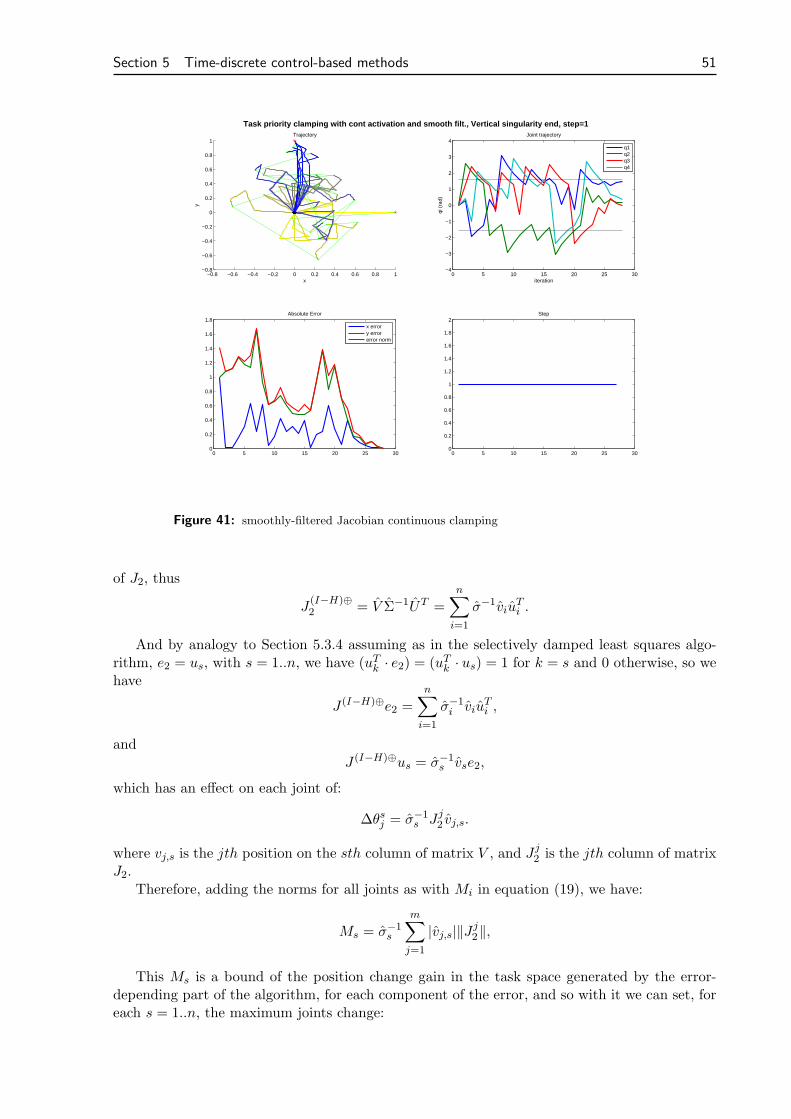
Section 5 Time-discrete control-based methods 51
−0.8 −0.6 −0.4 −0.2 0 0.2 0.4 0.6 0.8 1−0.8
−0.6
−0.4
−0.2
0
0.2
0.4
0.6
0.8
1Trajectory
x
y
0 5 10 15 20 25 30−4
−3
−2
−1
0
1
2
3
4
iteration
qi (
rad)
Joint trajectory
q1q2q3q4
0 5 10 15 20 25 300
0.2
0.4
0.6
0.8
1
1.2
1.4
1.6
1.8Absolute Error
x errory errorerror norm
Task priority clamping with cont activation and smooth filt., Vertical singularity end, step=1
0 5 10 15 20 25 300
0.2
0.4
0.6
0.8
1
1.2
1.4
1.6
1.8
2Step
Figure 41: smoothly-filtered Jacobian continuous clamping
of J2, thus
J(I−H)⊕2 = V Σ−1UT =
n∑
i=1
σ−1viuTi .
And by analogy to Section 5.3.4 assuming as in the selectively damped least squares algo-rithm, e2 = us, with s = 1..n, we have (uTk · e2) = (uTk · us) = 1 for k = s and 0 otherwise, so wehave
J (I−H)⊕e2 =n∑
i=1
σ−1i viu
Ti ,
andJ (I−H)⊕us = σ−1
s vse2,
which has an effect on each joint of:
∆θsj = σ−1s J j
2 vj,s.
where vj,s is the jth position on the sth column of matrix V , and J j2 is the jth column of matrix
J2.Therefore, adding the norms for all joints as with Mi in equation (19), we have:
Ms = σ−1s
m∑
j=1
|vj,s|‖J j2‖,
This Ms is a bound of the position change gain in the task space generated by the error-depending part of the algorithm, for each component of the error, and so with it we can set, foreach s = 1..n, the maximum joints change:
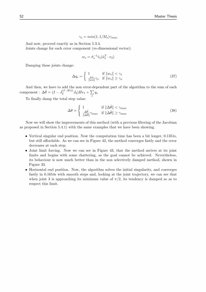
52 Master Thesis
γs = min(1, 1/Ms)γmax
And now, proceed exactly as in Section 5.3.4.Joints change for each error component (m-dimensional vector):
ws = σ−1s vs(u
Ts · e2)
Damping these joints change:
∆qs =
{
1 if ‖ws‖ < γsws
‖ws‖γs if ‖ws‖ ≥ γs(37)
And then, we have to add the non error-dependent part of the algorithm to the sum of each
component : ∆θ = (I − J(I−H)⊕2 J2)He1 +
∑
sqs
To finally damp the total step value:
∆θ =
{
1 if ‖∆θ‖ < γmax
∆θ‖∆θ‖
γmax if ‖∆θ‖ ≥ γmax(38)
Now we will show the improvements of this method (with a previous filtering of the Jacobianas proposed in Section 5.4.1) with the same examples that we have been showing.
• Vertical singular end position. Now the computation time has been a bit longer, 0.1351s,but still affordable. As we can see in Figure 42, the method converges fastly and the errordecreases at each step.
• Joint limit forcing. Now we can see in Figure 43, that the method arrives at its jointlimits and begins with some chattering, as the goal cannot be achieved. Nevertheless,its behaviour is now much better than in the non selectively damped method, shown inFigure 33.
• Horizontal end position. Now, the algorithm solves the initial singularity, and convergesfastly in 0.1654s with smooth steps and, looking at the joint trajectory, we can see thatwhen joint 3 is approaching its minimum value of π/2, its tendency is damped so as torespect this limit.
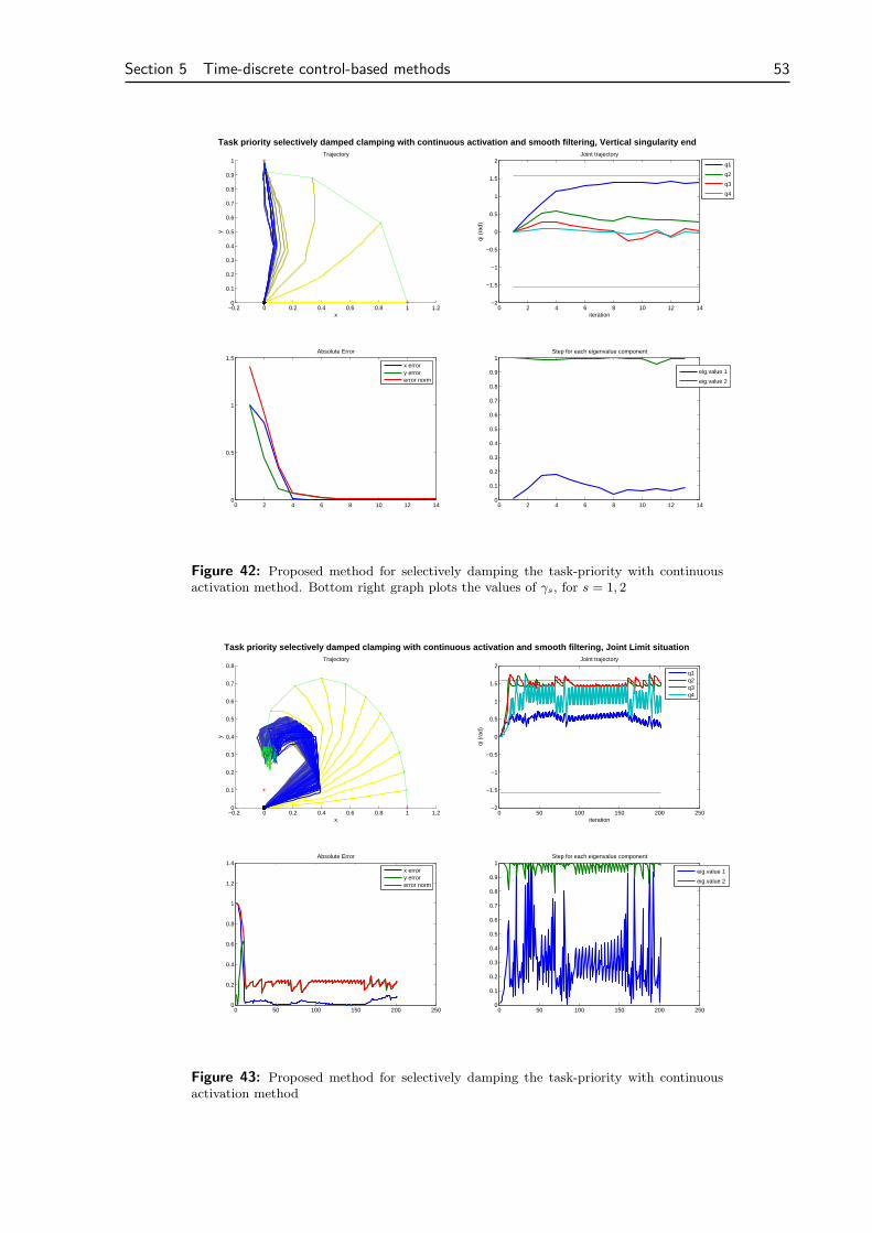
Section 5 Time-discrete control-based methods 53
−0.2 0 0.2 0.4 0.6 0.8 1 1.20
0.1
0.2
0.3
0.4
0.5
0.6
0.7
0.8
0.9
1Trajectory
x
y
0 2 4 6 8 10 12 14−2
−1.5
−1
−0.5
0
0.5
1
1.5
2
iteration
qi (
rad)
Joint trajectory
q1
q2
q3
q4
0 2 4 6 8 10 12 140
0.5
1
1.5Absolute Error
x errory errorerror norm
Task priority selectively damped clamping with continuous activation and smooth filtering, Vertical singularity end
0 2 4 6 8 10 12 140
0.1
0.2
0.3
0.4
0.5
0.6
0.7
0.8
0.9
1Step for each eigenvalue component
eig.value 1
eig.value 2
Figure 42: Proposed method for selectively damping the task-priority with continuousactivation method. Bottom right graph plots the values of γs, for s = 1, 2
−0.2 0 0.2 0.4 0.6 0.8 1 1.20
0.1
0.2
0.3
0.4
0.5
0.6
0.7
0.8Trajectory
x
y
0 50 100 150 200 250−2
−1.5
−1
−0.5
0
0.5
1
1.5
2
iteration
qi (
rad)
Joint trajectory
q1q2q3q4
0 50 100 150 200 2500
0.2
0.4
0.6
0.8
1
1.2
1.4Absolute Error
x errory errorerror norm
Task priority selectively damped clamping with continuous activation and smooth filtering, Joint Limit situation
0 50 100 150 200 2500
0.1
0.2
0.3
0.4
0.5
0.6
0.7
0.8
0.9
1Step for each eigenvalue component
eig.value 1
eig.value 2
Figure 43: Proposed method for selectively damping the task-priority with continuousactivation method
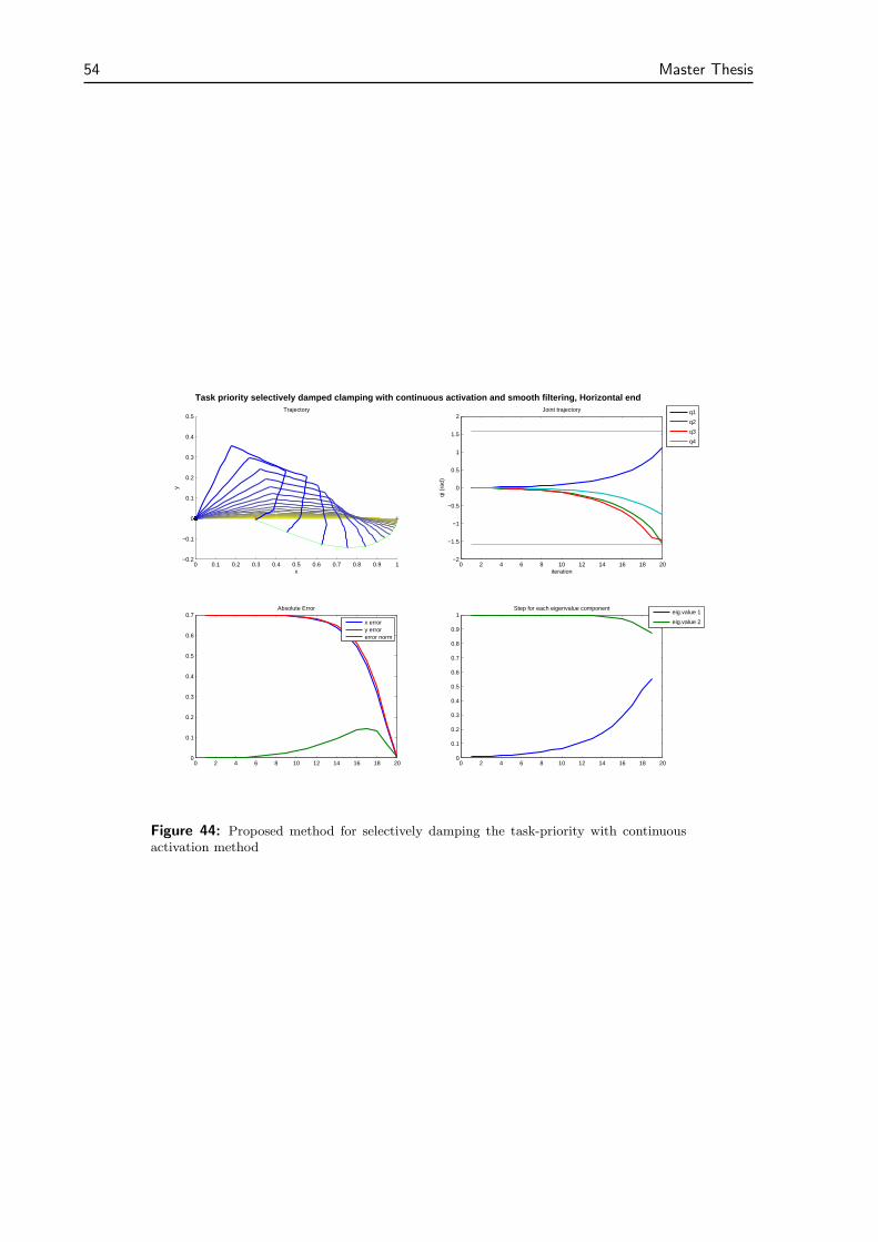
54 Master Thesis
0 0.1 0.2 0.3 0.4 0.5 0.6 0.7 0.8 0.9 1−0.2
−0.1
0
0.1
0.2
0.3
0.4
0.5Trajectory
x
y
0 2 4 6 8 10 12 14 16 18 20−2
−1.5
−1
−0.5
0
0.5
1
1.5
2
iteration
qi (
rad)
Joint trajectory
q1
q2
q3
q4
0 2 4 6 8 10 12 14 16 18 200
0.1
0.2
0.3
0.4
0.5
0.6
0.7Absolute Error
x errory errorerror norm
Task priority selectively damped clamping with continuous activation and smooth filtering, Horizontal end
0 2 4 6 8 10 12 14 16 18 200
0.1
0.2
0.3
0.4
0.5
0.6
0.7
0.8
0.9
1Step for each eigenvalue component
eig.value 1
eig.value 2
Figure 44: Proposed method for selectively damping the task-priority with continuousactivation method

Section 5 Time-discrete control-based methods 55
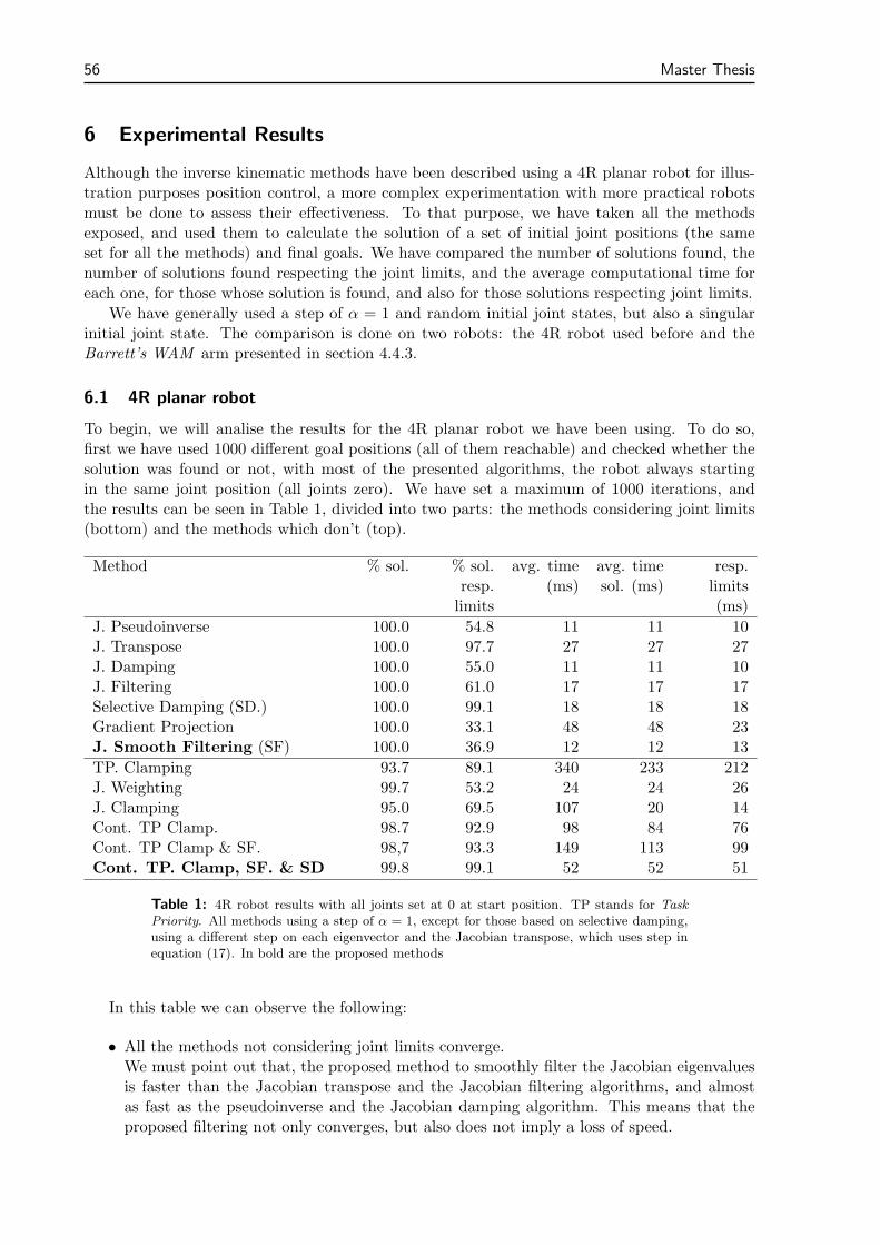
56 Master Thesis
6 Experimental Results
Although the inverse kinematic methods have been described using a 4R planar robot for illus-tration purposes position control, a more complex experimentation with more practical robotsmust be done to assess their effectiveness. To that purpose, we have taken all the methodsexposed, and used them to calculate the solution of a set of initial joint positions (the sameset for all the methods) and final goals. We have compared the number of solutions found, thenumber of solutions found respecting the joint limits, and the average computational time foreach one, for those whose solution is found, and also for those solutions respecting joint limits.
We have generally used a step of α = 1 and random initial joint states, but also a singularinitial joint state. The comparison is done on two robots: the 4R robot used before and theBarrett’s WAM arm presented in section 4.4.3.
6.1 4R planar robot
To begin, we will analise the results for the 4R planar robot we have been using. To do so,first we have used 1000 different goal positions (all of them reachable) and checked whether thesolution was found or not, with most of the presented algorithms, the robot always startingin the same joint position (all joints zero). We have set a maximum of 1000 iterations, andthe results can be seen in Table 1, divided into two parts: the methods considering joint limits(bottom) and the methods which don’t (top).
Method % sol. % sol.resp.limits
avg. time(ms)
avg. timesol. (ms)
resp.limits(ms)
J. Pseudoinverse 100.0 54.8 11 11 10J. Transpose 100.0 97.7 27 27 27J. Damping 100.0 55.0 11 11 10J. Filtering 100.0 61.0 17 17 17Selective Damping (SD.) 100.0 99.1 18 18 18Gradient Projection 100.0 33.1 48 48 23J. Smooth Filtering (SF) 100.0 36.9 12 12 13
TP. Clamping 93.7 89.1 340 233 212J. Weighting 99.7 53.2 24 24 26J. Clamping 95.0 69.5 107 20 14Cont. TP Clamp. 98.7 92.9 98 84 76Cont. TP Clamp & SF. 98,7 93.3 149 113 99Cont. TP. Clamp, SF. & SD 99.8 99.1 52 52 51
Table 1: 4R robot results with all joints set at 0 at start position. TP stands for Task
Priority. All methods using a step of α = 1, except for those based on selective damping,using a different step on each eigenvector and the Jacobian transpose, which uses step inequation (17). In bold are the proposed methods
In this table we can observe the following:
• All the methods not considering joint limits converge.We must point out that, the proposed method to smoothly filter the Jacobian eigenvaluesis faster than the Jacobian transpose and the Jacobian filtering algorithms, and almostas fast as the pseudoinverse and the Jacobian damping algorithm. This means that theproposed filtering not only converges, but also does not imply a loss of speed.
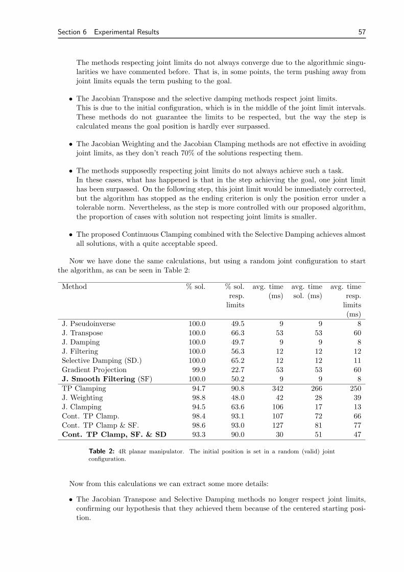
Section 6 Experimental Results 57
The methods respecting joint limits do not always converge due to the algorithmic singu-larities we have commented before. That is, in some points, the term pushing away fromjoint limits equals the term pushing to the goal.
• The Jacobian Transpose and the selective damping methods respect joint limits.This is due to the initial configuration, which is in the middle of the joint limit intervals.These methods do not guarantee the limits to be respected, but the way the step iscalculated means the goal position is hardly ever surpassed.
• The Jacobian Weighting and the Jacobian Clamping methods are not effective in avoidingjoint limits, as they don’t reach 70% of the solutions respecting them.
• The methods supposedly respecting joint limits do not always achieve such a task.In these cases, what has happened is that in the step achieving the goal, one joint limithas been surpassed. On the following step, this joint limit would be inmediately corrected,but the algorithm has stopped as the ending criterion is only the position error under atolerable norm. Nevertheless, as the step is more controlled with our proposed algorithm,the proportion of cases with solution not respecting joint limits is smaller.
• The proposed Continuous Clamping combined with the Selective Damping achieves almostall solutions, with a quite acceptable speed.
Now we have done the same calculations, but using a random joint configuration to startthe algorithm, as can be seen in Table 2:
Method % sol. % sol.resp.limits
avg. time(ms)
avg. timesol. (ms)
avg. timeresp.limits(ms)
J. Pseudoinverse 100.0 49.5 9 9 8J. Transpose 100.0 66.3 53 53 60J. Damping 100.0 49.7 9 9 8J. Filtering 100.0 56.3 12 12 12Selective Damping (SD.) 100.0 65.2 12 12 11Gradient Projection 99.9 22.7 53 53 60J. Smooth Filtering (SF) 100.0 50.2 9 9 8
TP Clamping 94.7 90.8 342 266 250J. Weighting 98.8 48.0 42 28 39J. Clamping 94.5 63.6 106 17 13Cont. TP Clamp. 98.4 93.1 107 72 66Cont. TP Clamp & SF. 98.6 93.0 127 81 77Cont. TP Clamp, SF. & SD 93.3 90.0 30 51 47
Table 2: 4R planar manipulator. The initial position is set in a random (valid) jointconfiguration.
Now from this calculations we can extract some more details:
• The Jacobian Transpose and Selective Damping methods no longer respect joint limits,confirming our hypothesis that they achieved them because of the centered starting posi-tion.
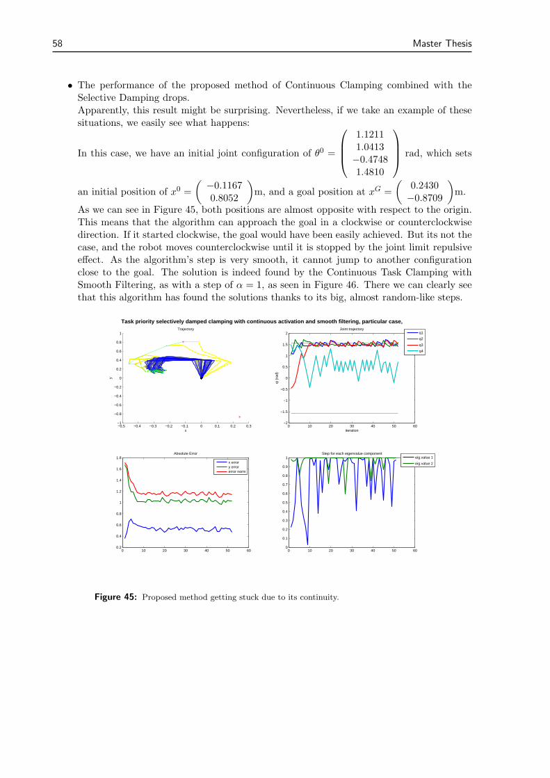
58 Master Thesis
• The performance of the proposed method of Continuous Clamping combined with theSelective Damping drops.Apparently, this result might be surprising. Nevertheless, if we take an example of thesesituations, we easily see what happens:
In this case, we have an initial joint configuration of θ0 =
1.12111.0413−0.47481.4810
rad, which sets
an initial position of x0 =
(
−0.11670.8052
)
m, and a goal position at xG =
(
0.2430−0.8709
)
m.
As we can see in Figure 45, both positions are almost opposite with respect to the origin.This means that the algorithm can approach the goal in a clockwise or counterclockwisedirection. If it started clockwise, the goal would have been easily achieved. But its not thecase, and the robot moves counterclockwise until it is stopped by the joint limit repulsiveeffect. As the algorithm’s step is very smooth, it cannot jump to another configurationclose to the goal. The solution is indeed found by the Continuous Task Clamping withSmooth Filtering, as with a step of α = 1, as seen in Figure 46. There we can clearly seethat this algorithm has found the solutions thanks to its big, almost random-like steps.
−0.5 −0.4 −0.3 −0.2 −0.1 0 0.1 0.2 0.3−1
−0.8
−0.6
−0.4
−0.2
0
0.2
0.4
0.6
0.8
1Trajectory
x
y
0 10 20 30 40 50 60−2
−1.5
−1
−0.5
0
0.5
1
1.5
2
iteration
qi (
rad)
Joint trajectory
q1
q2
q3
q4
0 10 20 30 40 50 600.2
0.4
0.6
0.8
1
1.2
1.4
1.6
1.8Absolute Error
x errory errorerror norm
Task priority selectively damped clamping with continuous activation and smooth filtering, particular case,
0 10 20 30 40 50 600
0.1
0.2
0.3
0.4
0.5
0.6
0.7
0.8
0.9
1Step for each eigenvalue component
eig.value 1
eig.value 2
Figure 45: Proposed method getting stuck due to its continuity.
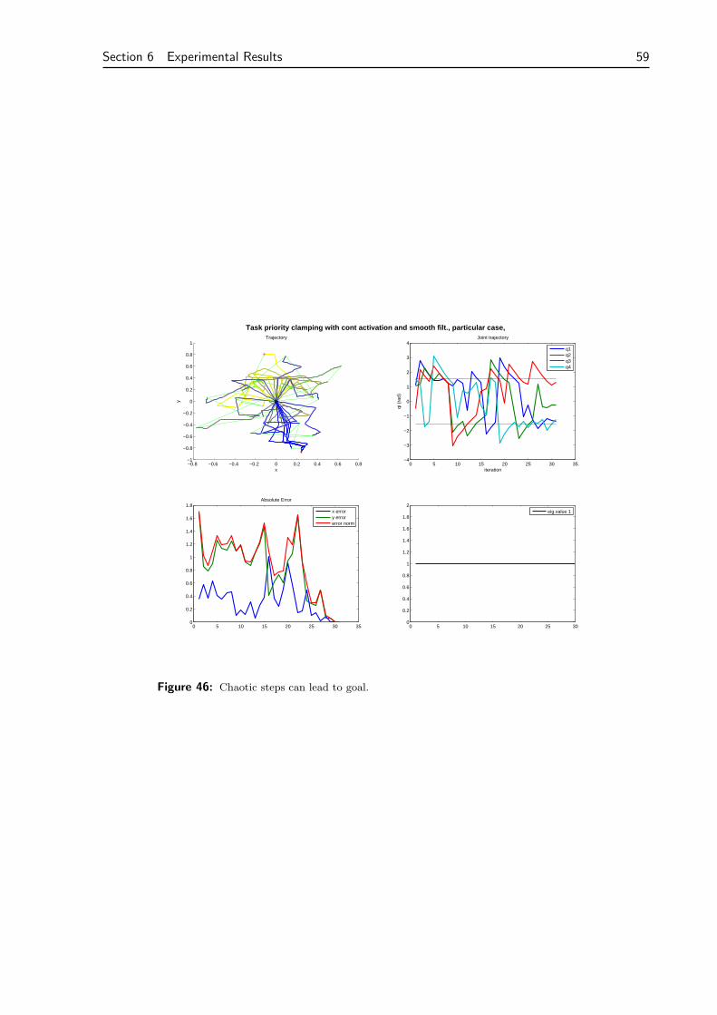
Section 6 Experimental Results 59
−0.8 −0.6 −0.4 −0.2 0 0.2 0.4 0.6 0.8−1
−0.8
−0.6
−0.4
−0.2
0
0.2
0.4
0.6
0.8
1Trajectory
x
y
0 5 10 15 20 25 30 35−4
−3
−2
−1
0
1
2
3
4
iteration
qi (
rad)
Joint trajectory
q1q2q3q4
0 5 10 15 20 25 30 350
0.2
0.4
0.6
0.8
1
1.2
1.4
1.6
1.8Absolute Error
x errory errorerror norm
Task priority clamping with cont activation and smooth filt., particular case,
0 5 10 15 20 25 300
0.2
0.4
0.6
0.8
1
1.2
1.4
1.6
1.8
2
eig.value 1
Figure 46: Chaotic steps can lead to goal.
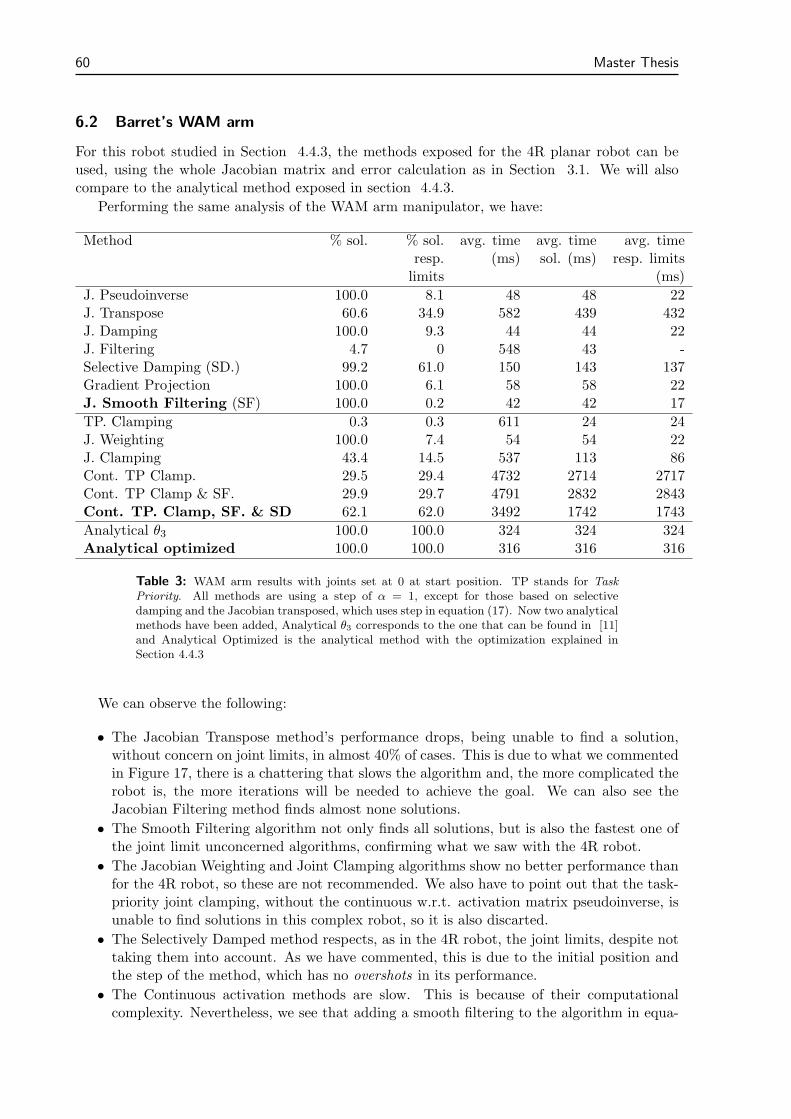
60 Master Thesis
6.2 Barret’s WAM arm
For this robot studied in Section 4.4.3, the methods exposed for the 4R planar robot can beused, using the whole Jacobian matrix and error calculation as in Section 3.1. We will alsocompare to the analytical method exposed in section 4.4.3.
Performing the same analysis of the WAM arm manipulator, we have:
Method % sol. % sol.resp.limits
avg. time(ms)
avg. timesol. (ms)
avg. timeresp. limits
(ms)
J. Pseudoinverse 100.0 8.1 48 48 22J. Transpose 60.6 34.9 582 439 432J. Damping 100.0 9.3 44 44 22J. Filtering 4.7 0 548 43 -Selective Damping (SD.) 99.2 61.0 150 143 137Gradient Projection 100.0 6.1 58 58 22J. Smooth Filtering (SF) 100.0 0.2 42 42 17
TP. Clamping 0.3 0.3 611 24 24J. Weighting 100.0 7.4 54 54 22J. Clamping 43.4 14.5 537 113 86Cont. TP Clamp. 29.5 29.4 4732 2714 2717Cont. TP Clamp & SF. 29.9 29.7 4791 2832 2843Cont. TP. Clamp, SF. & SD 62.1 62.0 3492 1742 1743
Analytical θ3 100.0 100.0 324 324 324Analytical optimized 100.0 100.0 316 316 316
Table 3: WAM arm results with joints set at 0 at start position. TP stands for Task
Priority. All methods are using a step of α = 1, except for those based on selectivedamping and the Jacobian transposed, which uses step in equation (17). Now two analyticalmethods have been added, Analytical θ3 corresponds to the one that can be found in [11]and Analytical Optimized is the analytical method with the optimization explained inSection 4.4.3
We can observe the following:
• The Jacobian Transpose method’s performance drops, being unable to find a solution,without concern on joint limits, in almost 40% of cases. This is due to what we commentedin Figure 17, there is a chattering that slows the algorithm and, the more complicated therobot is, the more iterations will be needed to achieve the goal. We can also see theJacobian Filtering method finds almost none solutions.
• The Smooth Filtering algorithm not only finds all solutions, but is also the fastest one ofthe joint limit unconcerned algorithms, confirming what we saw with the 4R robot.
• The Jacobian Weighting and Joint Clamping algorithms show no better performance thanfor the 4R robot, so these are not recommended. We also have to point out that the task-priority joint clamping, without the continuous w.r.t. activation matrix pseudoinverse, isunable to find solutions in this complex robot, so it is also discarted.
• The Selectively Damped method respects, as in the 4R robot, the joint limits, despite nottaking them into account. As we have commented, this is due to the initial position andthe step of the method, which has no overshots in its performance.
• The Continuous activation methods are slow. This is because of their computationalcomplexity. Nevertheless, we see that adding a smooth filtering to the algorithm in equa-
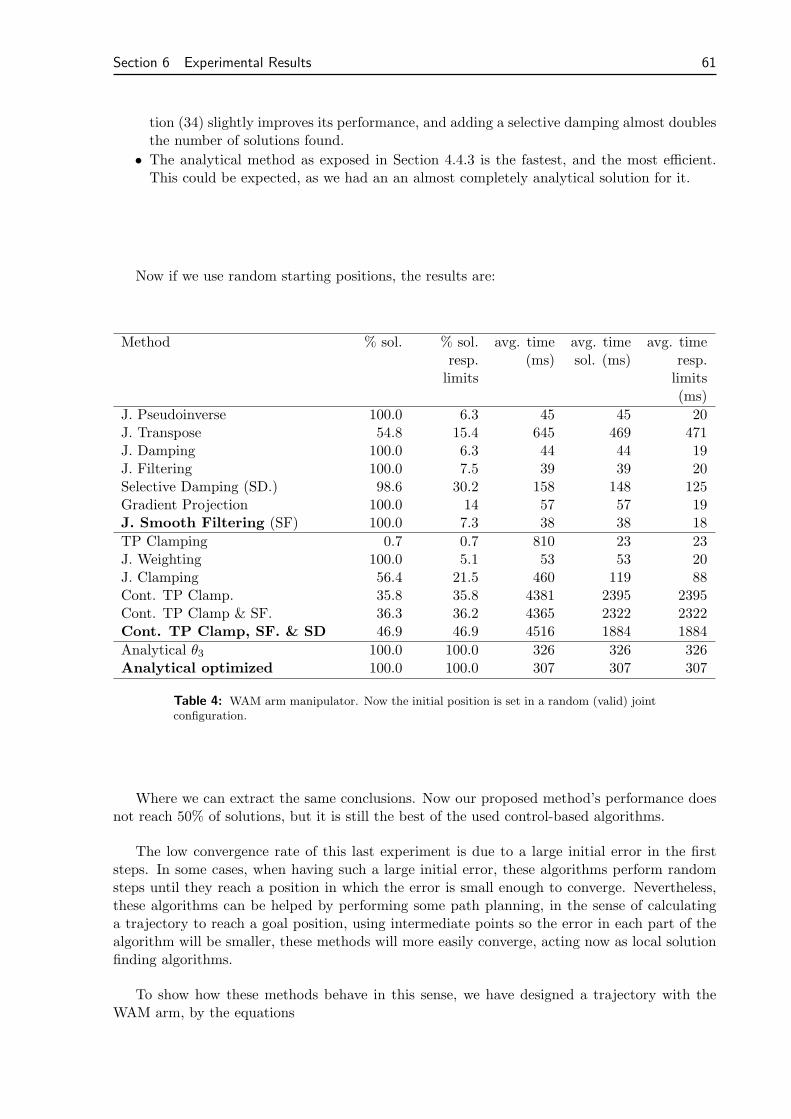
Section 6 Experimental Results 61
tion (34) slightly improves its performance, and adding a selective damping almost doublesthe number of solutions found.
• The analytical method as exposed in Section 4.4.3 is the fastest, and the most efficient.This could be expected, as we had an an almost completely analytical solution for it.
Now if we use random starting positions, the results are:
Method % sol. % sol.resp.limits
avg. time(ms)
avg. timesol. (ms)
avg. timeresp.limits(ms)
J. Pseudoinverse 100.0 6.3 45 45 20J. Transpose 54.8 15.4 645 469 471J. Damping 100.0 6.3 44 44 19J. Filtering 100.0 7.5 39 39 20Selective Damping (SD.) 98.6 30.2 158 148 125Gradient Projection 100.0 14 57 57 19J. Smooth Filtering (SF) 100.0 7.3 38 38 18
TP Clamping 0.7 0.7 810 23 23J. Weighting 100.0 5.1 53 53 20J. Clamping 56.4 21.5 460 119 88Cont. TP Clamp. 35.8 35.8 4381 2395 2395Cont. TP Clamp & SF. 36.3 36.2 4365 2322 2322Cont. TP Clamp, SF. & SD 46.9 46.9 4516 1884 1884
Analytical θ3 100.0 100.0 326 326 326Analytical optimized 100.0 100.0 307 307 307
Table 4: WAM arm manipulator. Now the initial position is set in a random (valid) jointconfiguration.
Where we can extract the same conclusions. Now our proposed method’s performance doesnot reach 50% of solutions, but it is still the best of the used control-based algorithms.
The low convergence rate of this last experiment is due to a large initial error in the firststeps. In some cases, when having such a large initial error, these algorithms perform randomsteps until they reach a position in which the error is small enough to converge. Nevertheless,these algorithms can be helped by performing some path planning, in the sense of calculatinga trajectory to reach a goal position, using intermediate points so the error in each part of thealgorithm will be smaller, these methods will more easily converge, acting now as local solutionfinding algorithms.
To show how these methods behave in this sense, we have designed a trajectory with theWAM arm, by the equations
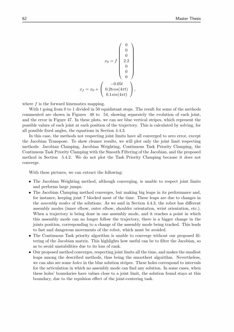
62 Master Thesis
x0 = f
0002.2000
xf = x0 +
−0.05t0.2tcos(4πt)0.1sin(4πt)
,
where f is the forward kinematics mapping.With t going from 0 to 1 divided in 50 equidistant steps. The result for some of the methods
commented are shown in Figures 48 to 54, showing separately the evolution of each joint,and the error in Figure 47. In these plots, we can see blue vertical stripes, which represent thepossible values of each joint at each position of the trajectory. This is calculated by solving, forall possible fixed angles, the equations in Section 4.4.3.
In this case, the methods not respecting joint limits have all converged to zero error, exceptthe Jacobian Transpose. To show cleaner results, we will plot only the joint limit respectingmethods: Jacobian Clamping, Jacobian Weighting, Continuous Task Priority Clamping, theContinuous Task Priority Clamping with the Smooth Filtering of the Jacobian, and the proposedmethod in Section 5.4.2. We do not plot the Task Priority Clamping because it does notconverge.
With these pictures, we can extract the following:
• The Jacobian Weighting method, although converging, is unable to respect joint limitsand performs large jumps.
• The Jacobian Clamping method converges, but making big leaps in its performance and,for instance, keeping joint 7 blocked most of the time. These leaps are due to changes inthe assembly modes of the solutions. As we said in Section 4.4.3, the robot has differentassembly modes (inner elbow, outer elbow, shoulder orientation, wrist orientation, etc.).When a trajectory is being done in one assembly mode, and it reaches a point in whichthis assembly mode can no longer follow the trajectory, there is a bigger change in thejoints position, corresponding to a change of the assembly mode being tracked. This leadsto fast and dangerous movements of the robot, which must be avoided.
• The Continuous Task priority algorithm is unable to converge without our proposed fil-tering of the Jacobian matrix. This highlights how useful can be to filter the Jacobian, soas to avoid unstabilities due to its loss of rank.
• Our proposed method converges, respecting joint limits all the time, and makes the smallestleaps among the described methods, thus being the smoothest algorithm. Nevertheless,we can also see some holes in the blue solution stripes. These holes correspond to intervalsfor the articulation in which no assembly mode can find any solution. In some cases, whenthese holes’ boundaries have values close to a joint limit, the solution found stays at thisboundary, due to the repulsion effect of the joint-centering task.
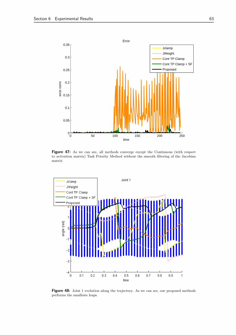
Section 6 Experimental Results 63
0 50 100 150 200 2500
0.05
0.1
0.15
0.2
0.25
0.3
0.35Error
time
erro
r no
rm
Jclamp
JWeight
Cont TP Clamp
Cont TP Clamp + SF
Proposed
Figure 47: As we can see, all methods converge except the Continuous (with respectto activation matrix) Task Priority Method without the smooth filtering of the Jacobianmatrix
Figure 48: Joint 1 evolution along the trajectory. As we can see, our proposed methodsperforms the smallests leaps.
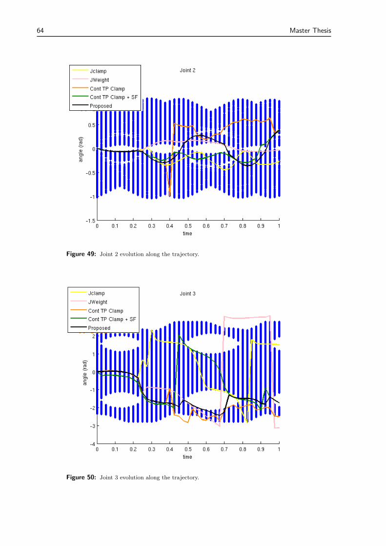
64 Master Thesis
Figure 49: Joint 2 evolution along the trajectory.
Figure 50: Joint 3 evolution along the trajectory.
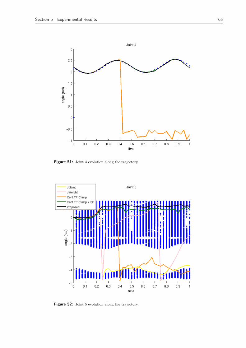
Section 6 Experimental Results 65
Figure 51: Joint 4 evolution along the trajectory.
Figure 52: Joint 5 evolution along the trajectory.
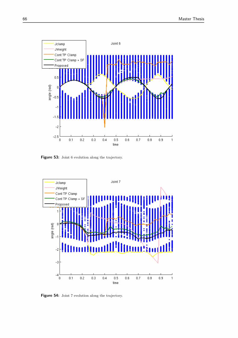
66 Master Thesis
Figure 53: Joint 6 evolution along the trajectory.
Figure 54: Joint 7 evolution along the trajectory.

Section 6 Experimental Results 67
68 Master Thesis
7 Conclusions and Future Work
Along this work, we have exposed the most popular of the inverse kinematic control-basedalgorithms in a survey-like way, clearly pointing their pros and contras. We have also proposedtwo ways of improving these methods:
• Analytical methods are usually faster. With the example of the WAM arm, we have clearlyseen that analytical methods are always a good solution when available. In this case, forthe WAM arm, we could find such a solution, but for the case of the 4R manipulator, wereit is harder to determine it, or for the laparoscopic robot commented, alternative methodssuch as control-based ones are a good option.
• Efficiently filtering the Jacobian matrix of a manipulator.As exposed in Section 5.4.1, we proved theoretically and in practice that our proposalimproves the existing methods to numerically filter or damp the Jacobian pseudoinverseof a matrix. We have also seen that this does not mean an additional computationalcost to the algorithm. With this filtering, the Jacobian matrix can be assumed to alwaysbe full ranked, without generating much additional error on the algorithms, thus thepseudoinverse operator does not have discontinuities due to a rank change in the Jacobianmatrix. This can be used in all control-based methods so as to improve their performance.
• A smooth inverse kinematic method.Smooth not only in its dependency on the rank of the Jacobian matrix, but also in itsactivation matrices to avoid joint limits, thanks to the work done at [14]. Also, its step,different for each eigenvector of the task, using what was proposed in [2], avoids largegains on each iteration. This method combines the advantages of other existing proceduresto approach the target position smoothly, eliminating any random-like behaviour, withthe drawback that being smooth means it cannot find the solution by chance, as thosewith a large step can do when the initial error is too large. This proposed algorithm mightperform even better in relation to the other algorithms seen when using it as a positiononline control algorithm, or a local optimizing algorithm as it is robust with respect to theerror, respects joint limits, and calculates its step at each iteration. More secondary taskscan also be added with a task priority structure, to improve the obtained position.
As stated in [7], the convergence of control-based methods strongly depends on their step αand their initial error e0. If α is set as a constant and the initial error is large, then these methodsperform oriented jumps until they reach a position in which the error is small enough to make themethod converge with the given α. In fact, this behaviour could be linked with pseudo-randomplanning algorithms such as the Rapidly-exploring Random Tree algorithm. When used as localplanners for complex robots, although their convergence improves, it cannot be assured withoutconsidering the iteration step α, and these methods easily jump from one assembly mode toanother, causing dangerous moves of the manipulator if controlled online. Our proposed methodreduces these drawbacks.
From here, our future work on it could be oriented in the following directions:
• Add other optimization tasks on the proposed algorithm, such a manipulability optimiza-tion.
• Reduce computational cost, possibly by tuning parameters and improving the algorithms.
• Avoid the algorithm to take bad decisions as in Figure 45. This issue might lead to thepath planning field.

Section 7 Conclusions and Future Work 69
70 REFERENCES
References
[1] J. Baillieul. Kinematic programming alternatives for redundant manipulators. In Proceed-ings. 1985 IEEE International Conference on Robotics and Automation., volume 2, pages722–728, mar 1985.
[2] Samuel R. Buss and Jin-Su Kim. Selectively damped least squares for inverse kinematics.Journal of Graphics Tools, 10:37–49, 2004.
[3] Tan Fung Chan and R.V. Dubey. A weighted least-norm solution based scheme for avoidingjoint limits for redundant joint manipulators. IEEE Transactions on Robotics and Automa-tion, 11(2):286–292, apr 1995.
[4] S. Chiaverini. Singularity-robust task-priority redundancy resolution for real-time kinematiccontrol of robot manipulators. Robotics and Automation, IEEE Transactions on, 13(3):398–410, jun 1997.
[5] S. Chiaverini, O. Egeland, and R.K. Kanestrom. Achieving user-defined accuracy withdamped least-squares inverse kinematics. In Advanced Robotics, 1991. ’Robots in Unstruc-tured Environments’, 91 ICAR., Fifth International Conference on, pages 672–677 vol.1,jun 1991.
[6] S. Chiaverini, B. Siciliano, and O. Egeland. Review of the damped least-squares inversekinematics with experiments on an industrial robot manipulator. Control Systems Tech-nology, IEEE Transactions on, 2(2):123–134, jun 1994.
[7] P. Falco and C. Natale. On the stability of closed-loop inverse kinematics algorithms forredundant robots. Robotics, IEEE Transactions on, PP(99):1–5, 2011.
[8] Z Jiang. A converse lyapunov theorem for discrete-time systems with disturbances. Systems& Control Letters, 45:49–58, 2002.
[9] C.A. Klein, C. Chu-Jenq, and S. Ahmed. A new formulation of the extended jacobianmethod and its use in mapping algorithmic singularities for kinematically redundant ma-nipulators. Robotics and Automation, IEEE Transactions on, 11(1):50–55, feb 1995.
[10] Jihong Lee. A study on the manipulability measures for robot manipulators. In IntelligentRobots and Systems, 1997. IROS ’97., Proceedings of the 1997 IEEE/RSJ InternationalConference on, volume 3, pages 1458–1465 vol.3, sep 1997.
[11] T. Lozano-Perez and L. Kaelbling. Barrett wam/hand interface ros-pkg.http://code.google.com/p/lis-ros-pkg/.
[12] N. Mansard, O. Khatib, and A. Kheddar. A unified approach to integrate unilateral con-straints in the stack of tasks. Robotics, IEEE Transactions on, 25(3):670–685, june 2009.
[13] N. Mansard, A. Remazeilles, and F. Chaumette. Continuity of varying-feature-set control laws. Technical report, IRISA, 2007. Downloadable version atftp://ftp.irisa.fr/techreports/2007/PI-1864.pdf.
[14] N. Mansard, A. Remazeilles, and F. Chaumette. Continuity of varying-feature-set controllaws. Automatic Control, IEEE Transactions on, 54(11):2493–2505, nov. 2009.
[15] Josep M. Porta, Lluıs Ros, and Federico Thomas. Inverse kinematic solution of robot manip-ulators using interval analysis. 4th International Workshop on Computational Kinematics,2005.
REFERENCES 71
[16] R. S. Rao, A. Asaithambi, and S. K. Agrawal. Inverse kinematic solution of robot manip-ulators using interval analysis. Journal of Mechanical Design, 120(1):147–150, 1998.
[17] D. Raunhardt and R. Boulic. Progressive clamping. In Robotics and Automation, 2007IEEE International Conference on, pages 4414–4419, april 2007.
[18] M. Shimizu, H. Kakuya, W.-K. Yoon, K. Kitagaki, and K. Kosuge. Analytical inverse kine-matic computation for 7-dof redundant manipulators with joint limits and its applicationto redundancy resolution. Robotics, IEEE Transactions on, 24(5):1131–1142, oct. 2008.
[19] B. Siciliano and J.-J.E. Slotine. A general framework for managing multiple tasks in highlyredundant robotic systems. In Advanced Robotics, 1991. ’Robots in Unstructured Environ-ments’, 91 ICAR., Fifth International Conference on, pages 1211–1216 vol.2, jun 1991.
[20] Bruno Siciliano, Lorenzo Sciavicco, Luifi Villani, and Giuseppe Oriolo. Robotics. Modelling,Planning and Control. Advanced Textbooks in Control and Signal Processing. Springer,1st edition, 2009.
[21] G.K. Singh and J. Claassens. An analytical solution for the inverse kinematics of a redun-dant 7dof manipulator with link offsets. In Intelligent Robots and Systems (IROS), 2010IEEE/RSJ International Conference on, pages 2976–2982, oct. 2010.
[22] Sreenivas Tejomurtula and Subhash Kak. Inverse kinematics in robotics using neural net-works. Information Sciences, 116(2-4):147–164, 1999.
[23] D. E. Whitney. Resolved motion rate control of manipulators and human prostheses. InIEEE Transactions on Man-Machine Systems, 10, pages 47–53, 1969.
[24] W. A. Wolovich and H. Elliott. A computational technique for inverse kinematics. InDecision and Control, 1984. The 23rd IEEE Conference on, volume 23, pages 1359–1363,dec. 1984.
[25] T. Yoshikawa. Dynamic manipulability of robot manipulators. In Robotics and Automation.Proceedings. 1985 IEEE International Conference on, volume 2, pages 1033–1038, mar 1985.

72 REFERENCES


IRI reports
This report is in the series of IRI technical reports.All IRI technical reports are available for download at the IRI websitehttp://www.iri.upc.edu.