A human proof of Gessel's lattice path conjecture - … · A human proof of Gessel’s lattice path conjecture Alin Bostan, Irina Kurkova, Kilian Raschel To cite this version: Alin

A human proof of Gessel’s lattice path conjecture

Alin Bostan, Irina Kurkova, Kilian Raschel

To cite this version:

Alin Bostan, Irina Kurkova, Kilian Raschel. A human proof of Gessel’s lattice path conjec-ture. Transactions of the American Mathematical Society, American Mathematical Society,2016, 369 (2, February 2017), pp.1365-1393 <http://www.ams.org/journals/tran/0000-000-00/S0002-9947-2016-06804-X/>. <hal-00858083v3>

HAL Id: hal-00858083

https://hal.archives-ouvertes.fr/hal-00858083v3

Submitted on 13 Feb 2015

HAL is a multi-disciplinary open accessarchive for the deposit and dissemination of sci-entific research documents, whether they are pub-lished or not. The documents may come fromteaching and research institutions in France orabroad, or from public or private research centers.

L’archive ouverte pluridisciplinaire HAL, estdestinee au depot et a la diffusion de documentsscientifiques de niveau recherche, publies ou non,emanant des etablissements d’enseignement et derecherche francais ou etrangers, des laboratoirespublics ou prives.

Distributed under a Creative Commons Attribution 4.0 International License

https://hal.archives-ouvertes.fr

https://hal.archives-ouvertes.fr/hal-00858083v3

http://creativecommons.org/licenses/by/4.0/

http://creativecommons.org/licenses/by/4.0/

A HUMAN PROOF OF GESSEL’S LATTICE PATH CONJECTURE

A. BOSTAN, I. KURKOVA, AND K. RASCHEL

Abstract. Gessel walks are lattice paths confined to the quarter plane that start at the originand consist of unit steps going either West, East, South-West or North-East. In 2001, IraGessel conjectured a nice closed-form expression for the number of Gessel walks endingat the origin. In 2008, Kauers, Koutschan and Zeilberger gave a computer-aided proof ofthis conjecture. The same year, Bostan and Kauers showed, again using computer algebratools, that the complete generating function of Gessel walks is algebraic. In this article wepropose the first “human proofs” of these results. They are derived from a new expressionfor the generating function of Gessel walks in terms of Weierstrass zeta functions.

1. Introduction

Main results. Gessel walks are lattice paths confined to the quarter plane N2 =

{0, 1, 2, . . .} × {0, 1, 2, . . .}, that start at the origin (0, 0) and move by unit steps in oneof the following directions: West, East, South-West and North-East, see Figure 1. Gesselexcursions are those Gessel walks that return to the origin. For (i , j) ∈ N2 and n > 0, letq(i , j ; n) be the number of Gessel walks of length n ending at the point (i , j). Gessel walkshave been puzzling the combinatorics community since 2001, when Ira Gessel conjectured:

(A) For all n > 0, the following closed-form expression holds for the number of Gesselexcursions of even length 2n

q(0, 0; 2n) = 16n(5/6)n(1/2)n

(2)n(5/3)n, (1)

where (a)n = a(a + 1) · · · (a + n − 1) denotes the Pochhammer symbol.

Note that obviously there are no Gessel excursions of odd length, that is q(0, 0; 2n+ 1) = 0

for all n > 0. In 2008, Kauers, Koutschan and Zeilberger [19] provided a computer-aidedproof of this conjecture.

A second intriguing question was to decide whether or not:

Date: February 12, 2015.1991 Mathematics Subject Classification. Primary 05A15; Secondary 30F10, 30D05.Key words and phrases. Enumerative combinatorics; lattice paths; Gessel walks; generating functions;

algebraic functions; elliptic functions.A. Bostan: INRIA Saclay Île-de-France, Bâtiment Alan Turing, 1 rue Honoré d’Estienne d’Orves, 91120

Palaiseau, France.I. Kurkova: Laboratoire de Probabilités et Modèles Aléatoires, Université Pierre et Marie Curie, 4 Place

Jussieu, 75252 Paris Cedex 05, France.K. Raschel: CNRS & Fédération de recherche Denis Poisson & Laboratoire de Mathématiques et Physique

Théorique, Université de Tours, Parc de Grandmont, 37200 Tours, France.Emails: [email protected], [email protected], and [email protected].

fr.1

[email protected]

[email protected]

[email protected]

[email protected]

2 A. BOSTAN, I. KURKOVA, AND K. RASCHEL

-

6

��

��

-�

-� ��

-��

-��

-@@@

@@

@@@I

6

?

-�

�6-

-6

-6

Figure 1. On the left: allowed steps for Gessel walks. Note that on theboundary of N2, the steps that would take the walks out of N2 are discarded.On the right: an equivalent formulation of Gessel walks as the simple walksevolving in the cone with opening 135◦.

(B) Is the complete generating function (GF) of Gessel walks

Q(x, y ; z) =∑i ,j,n>0

q(i , j ; n)x iy jzn (2)

D-finite1, or even algebraic (i.e., root of a non-zero polynomial in Q(x, y , z)[T ])?

The answer to this question –namely, the (initially unexpected) algebraicity of Q(x, y ; z)–was finally obtained by Bostan and Kauers [4], using computer algebra techniques.

In summary, the only existing proofs for Problems (A) and (B) used heavycomputer calculations in a crucial way. In this article we obtain a newexplicit expression for Q(x, y ; z), from which we derive the first “humanproofs” of (A) and (B).

Context of Gessel’s conjecture. In 2001, the motivation for considering Gessel’s model ofwalks was twofold. First, by an obvious linear transformation, Gessel’s walk can be viewedas the simple walk (i.e., with allowed steps to the West, East, South and North) constrainedto lie in a cone with angle 135◦, see Figure 1. It turns out that before 2001, the simple walkwas well studied in different cones. Pólya [32] first considered the simple walk in the wholeplane (“drunkard’s walk”), and remarked that the probability that a simple random walk everreturns to the origin is equal to 1. This is a consequence of the fact that there are exactly(2nn

)2simple excursions of length 2n in the plane Z2. There also exist formulæ for simple

excursions of length 2n evolving in other regions of Z2:(2n+1n

)Cn for the half plane Z×N,

and CnCn+1 for the quarter plane N2, where Cn = 1n+1

(2nn

)is the Catalan number [2].

Gouyou-Beauchamps [16] found a similar formula CnCn+2 − C2n+1 for the number of simpleexcursions of length 2n in the cone with angle 45◦ (the first octant). It was thus natural toconsider the cone with angle 135◦, and this is what Gessel did.

The second part of the motivation is that Gessel’s model is a particular instance of walksin the quarter plane. In 2001 there were already several famous examples of such models:Kreweras’ walk [21, 13, 14, 6] (with allowed steps to the West, North-East and South)for which the GF (2) is algebraic; Gouyou-Beauchamps’s walk [16]; the simple walk [17].

1The function Q(x, y ; z) is called D-finite if the vector space over Q(x, y , z)—the field of rational functionsin the three variables x, y , z—spanned by the set of all partial derivatives of Q(x, y ; z) is finite-dimensional,see for instance [25].

A HUMAN PROOF OF GESSEL’S LATTICE PATH CONJECTURE 3

Further, around 2000, walks in the quarter plane were brought up to date, notably byBousquet-Mélou and Petkovšek [8, 9]. Indeed, they were used to illustrate the followingphenomenon: although the numbers of walks satisfy a (multivariate) linear recurrence withconstant coefficients, their GF (2) might be non-D-finite; see [9] for the example of theknight walk.

Existing results in the literature. After 2001, many approaches appeared for the treatmentof walks in the quarter plane. Bousquet-Mélou and Mishna initiated a systematic study ofsuch walks with small steps (this means that the step set, i.e., the set of allowed steps for thewalk, is a subset of the set of the eight nearest neighbors). Mishna [29, 30] first consideredthe case of step sets of cardinality three. She presented a complete classification of theGF (2) of these walks with respect to the classes of algebraic, transcendental D-finite andnon-D-finite power series. Bousquet-Mélou and Mishna [7] then explored all the 79 small stepsets2. They considered a functional equation for the GF that counts walks in such a modelleading to a group3 of birational transformations of C2. In 23 cases out of 79 this group turnsout to be finite, and the corresponding functional equations were solved in 22 out of 23 cases(the finiteness of the group being a crucial feature in [7]). The remaining case was preciselyGessel’s. In 2008, a method using computer algebra techniques was proposed by Kauers,Koutschan and Zeilberger [20, 19]. Kauers and Zeilberger [20] first obtained a computer-aided proof of the algebraicity of the GF counting Kreweras’ walks. A few months later,this approach was enhanced to cover Gessel’s case, and the conjecture (Problem (A)) wasproved [19]. At the same time, Bostan and Kauers [4] showed, again using heavy computercalculations, that the complete GF counting Gessel walks is algebraic (Problem (B)). Usingthe minimal polynomials obtained by Bostan and Kauers, van Hoeij [4, Appendix] managedto obtain an explicit and compact expression for the complete GF of Gessel walks.

Since the computerized proofs [19, 4], several computer-free analyses of the GF of Gesselwalks have been proposed [22, 34, 11, 3, 33, 36, 24], but none of them solved Gessel’sconjecture (Problem (A)), nor proved the algebraicity of the complete GF (Problem (B)).We briefly review the contributions of these works. Kurkova and Raschel [22] obtained anexplicit integral representation (a Cauchy integral) for Q(x, y ; z). This was done by solving aboundary value problem, a method inspired by the book [10]. It can be deduced from [22] thatthe generating function (2) is D-finite, since the Cauchy integral of an algebraic function isD-finite [31, 35]. This partially solves Problem (B). Nevertheless, the representation of [22]seems to be hardly accessible for further analyses, such as for expressing the coefficientsq(i , j ; n) in any satisfactory manner, and in particular for providing a proof of Gessel’sconjecture. This approach has been generalized subsequently for all models of walks withsmall steps in the quarter plane, see [34]. In [11], Fayolle and Raschel gave a proof ofthe algebraicity of the bivariate GF (partially solving Problem (B)), using probabilistic andalgebraic methods initiated in [10, Ch. 4]: more specifically, they proved that for any fixedvalue z0 ∈ (0, 1/4), the bivariate generating function Q(x, y ; z0) for Gessel walks is algebraicover R(x, y), hence over Q(x, y). The same approach gives the nature of the bivariate GF

2A priori, there are 28 = 256 step sets, but the authors of [7] showed that, after eliminating trivial cases,and also those which can be reduced to walks in a half plane, there remain 79 inherently different models.

3Historically, this group was introduced by Malyshev [26, 27, 28] in the seventies. For details on this groupwe refer to Section 2, in particular to equation (16).


in all the other 22 models with finite group. It is not possible to deduce Gessel’s conjectureusing the approach in [11], since it only uses the structure of the solutions of the functionalequation (3) satisfied by the generating function (2), but does not give access to any explicitexpression. Ayyer [3] proposed a combinatorial approach inspired by representation theory.He interpreted Gessel walks as words on certain alphabets. He then reformulated q(i , j ; n)

as numbers of words, and expressed very particular numbers of Gessel walks. Petkovšek andWilf [33] stated new conjectures, closely related to Gessel’s. They found an expression forGessel’s numbers in terms of determinants of matrices, by showing that the numbers of walksare solution to an infinite system of equations. Ping [36] introduced a probabilistic modelfor Gessel walks, and reduced the computation of q(i , j ; n) to the computation of a certainprobability. Using then probabilistic methods (such as the reflection principle) he provedtwo conjectures made by Petkovšek and Wilf in [33]. Very recently, using the Mittag-Lefflertheorem in a constructive way, Kurkova and Raschel [24] obtained new series expressions forthe GFs of all models of walks with small steps in the quarter plane, and worked out in detailthe case of Kreweras’ walks. The present article is strongly influenced by [24] and can beseen as a natural prolongation of it.

Presentation of our method and organization of the article. We fix z ∈ (0, 1/4). Tosolve Problems (A) and (B), we start from the GFs Q(x, 0; z) and Q(0, y ; z) and from thefunctional equation (see e.g. [7, §4.1])

K(x, y ; z)Q(x, y ; z) =

K(x, 0; z)Q(x, 0; z) +K(0, y ; z)Q(0, y ; z)−K(0, 0; z)Q(0, 0; z)− xy , ∀|x |, |y | < 1.

(3)

Above, K(x, y ; z) is the kernel of the walk, given by

K(x, y ; z) = xyz

∑(i ,j)∈G

x iy j − 1/z

= xyz(xy + x + 1/x + 1/(xy)− 1/z), (4)

where G = {(1, 1), (1, 0), (−1, 0), (−1,−1)} denotes Gessel’s step set (Figure 1).Rather than deriving an expression directly for the GFs Q(x, 0; z) and Q(0, y ; z), we shall

(equivalently) obtain expressions for Q(x(ω), 0; z) and Q(0, y(ω); z) for all ω ∈ Cω, whereCω denotes the complex plane, and where the functions x(ω) and y(ω) arise for reasonsthat we now present. This idea of introducing the ω-variable might appear unnecessarilycomplicated; in fact it is very natural, in the sense that many technical aspects of thereasonings will appear simple on the complex plane Cω (in particular, the group of the walk,the continuation of the GFs, their regularity, their explicit expressions, etc.).

We shall see in Section 2 that the elliptic curve defined by the zeros of the kernel

Tz = {(x, y) ∈ (C ∪ {∞})2 : K(x, y ; z) = 0} (5)

is of genus 1. This is a torus (constructed from two complex spheres properly glued together),or, equivalently, a parallelogram ω1[0, 1] + ω2[0, 1] whose opposite edges are identified. Itcan be parametrized by

Tz = {(x(ω), y(ω)) : ω ∈ C/(ω1Z+ ω2Z)}, (6)


••

•

•

•

• •−ω2 0

ω1

−ω1

2ω1

ω2 2ω2•

•

•0

ω1

ω2

-�

7ω2/8 > ω3

∆x ∆y

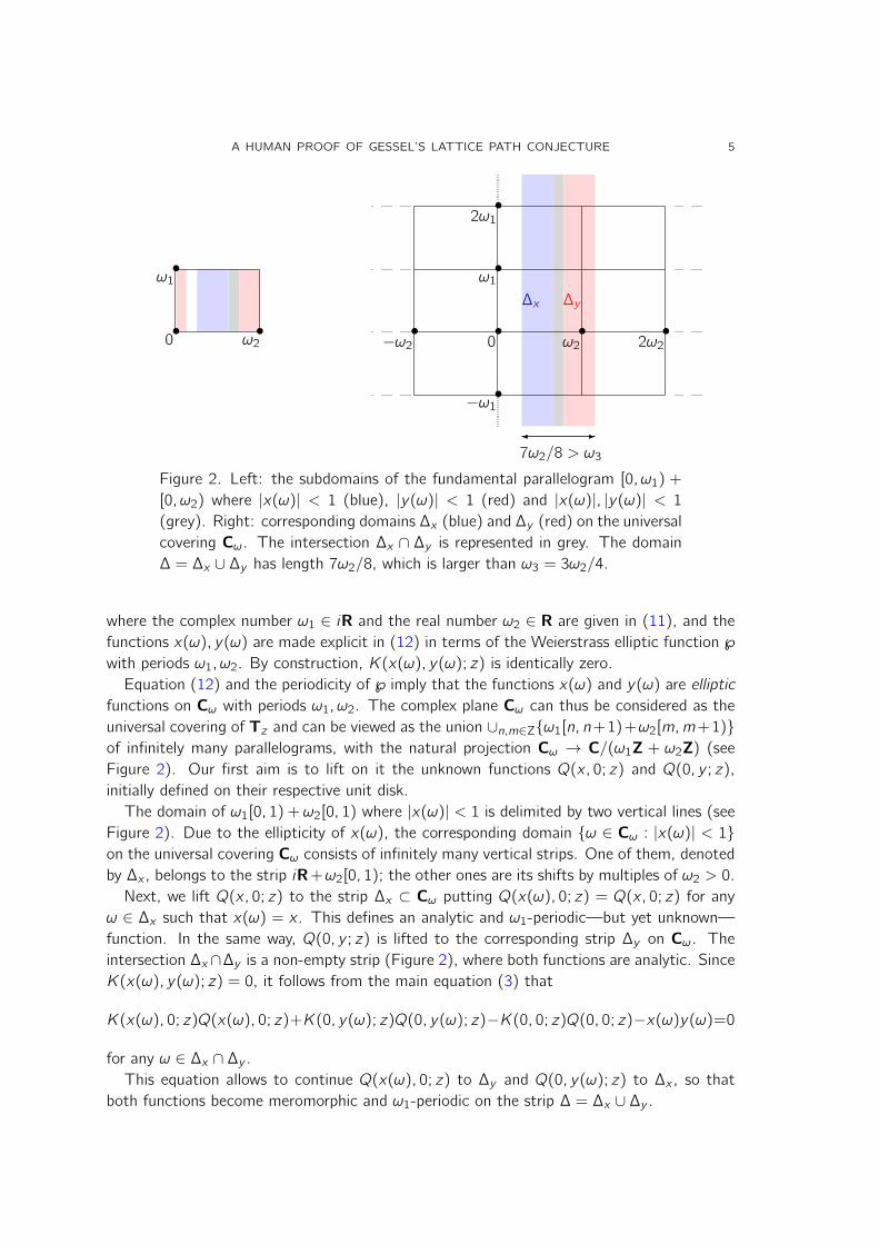
Figure 2. Left: the subdomains of the fundamental parallelogram [0, ω1) +

[0, ω2) where |x(ω)| < 1 (blue), |y(ω)| < 1 (red) and |x(ω)|, |y(ω)| < 1

(grey). Right: corresponding domains ∆x (blue) and ∆y (red) on the universalcovering Cω. The intersection ∆x ∩ ∆y is represented in grey. The domain∆ = ∆x ∪ ∆y has length 7ω2/8, which is larger than ω3 = 3ω2/4.

where the complex number ω1 ∈ iR and the real number ω2 ∈ R are given in (11), and thefunctions x(ω), y(ω) are made explicit in (12) in terms of the Weierstrass elliptic function ℘with periods ω1, ω2. By construction, K(x(ω), y(ω); z) is identically zero.

Equation (12) and the periodicity of ℘ imply that the functions x(ω) and y(ω) are ellipticfunctions on Cω with periods ω1, ω2. The complex plane Cω can thus be considered as theuniversal covering of Tz and can be viewed as the union ∪n,m∈Z{ω1[n, n+ 1) +ω2[m,m+ 1)}of infinitely many parallelograms, with the natural projection Cω → C/(ω1Z + ω2Z) (seeFigure 2). Our first aim is to lift on it the unknown functions Q(x, 0; z) and Q(0, y ; z),initially defined on their respective unit disk.

The domain of ω1[0, 1) + ω2[0, 1) where |x(ω)| < 1 is delimited by two vertical lines (seeFigure 2). Due to the ellipticity of x(ω), the corresponding domain {ω ∈ Cω : |x(ω)| < 1}on the universal covering Cω consists of infinitely many vertical strips. One of them, denotedby ∆x , belongs to the strip iR+ω2[0, 1); the other ones are its shifts by multiples of ω2 > 0.

Next, we lift Q(x, 0; z) to the strip ∆x ⊂ Cω putting Q(x(ω), 0; z) = Q(x, 0; z) for anyω ∈ ∆x such that x(ω) = x . This defines an analytic and ω1-periodic—but yet unknown—function. In the same way, Q(0, y ; z) is lifted to the corresponding strip ∆y on Cω. Theintersection ∆x ∩∆y is a non-empty strip (Figure 2), where both functions are analytic. SinceK(x(ω), y(ω); z) = 0, it follows from the main equation (3) that

K(x(ω), 0; z)Q(x(ω), 0; z)+K(0, y(ω); z)Q(0, y(ω); z)−K(0, 0; z)Q(0, 0; z)−x(ω)y(ω)=0

for any ω ∈ ∆x ∩ ∆y .This equation allows to continue Q(x(ω), 0; z) to ∆y and Q(0, y(ω); z) to ∆x , so that

both functions become meromorphic and ω1-periodic on the strip ∆ = ∆x ∪ ∆y .


The crucial point of our approach is the following: letting rx(ω) = K(x(ω), 0; z)Q(x(ω), 0; z),we have the key-identity

rx(ω − ω3) = rx(ω) + fx(ω), ∀ω ∈ Cω, (7)

where the shift vector ω3 = 3ω2/4 (real positive) and the function fx are explicit (andrelatively simple, see (14) and (23)). Equation (7) has many useful consequences:

(I) Due to (a repeated use of) (7), the function rx(ω) can bemeromorphically continuedfrom its initial domain of definition ∆ to the whole plane

Cω =⋃n∈Z{∆ + nω3}, (8)

see Section 2. By projecting back on Cx , we shall recover all branches of Q(x, 0; z).(II) We shall apply four times (7) and prove the identity fx(ω) + fx(ω + ω3) + fx(ω +

2ω3)+fx(ω+3ω3) = 0 (as we remark in Section 3, it exactly corresponds to the factthat the orbit sum of Gessel’s walks is zero, which was noticed in [7, Section 4.2]),from where we shall derive that rx is elliptic with periods (ω1, 4ω3), see Section 3.

(III) Since by (15) 4ω3 = 3ω2 (which is a non-trivial fact, and means that thegroup—to be defined in Section 2—of Gessel’s model has order 8), the theory oftransformations of elliptic functions will imply that rx is algebraic in the Weierstrassfunction ℘ with periods ω1, ω2. This will eventually yield the algebraicity of the GFQ(x, 0; z). Using a similar result for Q(0, y ; z) and the functional equation (3), weshall derive in this way the solution to Problem (B), see Section 5.

(IV) From (7) we shall also find the poles of rx and the principal parts at them. In general,it is clearly impossible to deduce the expression of a function from the knowledge ofits poles. A notable exception is constituted by elliptic functions, which is the caseof the function rx for Gessel walks, see (II) above. From this fact we shall deducean explicit expression of rx in terms of elliptic ζ-functions. By projection on Cx , thiswill give a new explicit expression of Q(x, 0; z) for Gessel walks as an infinite series.An analogous result will hold for Q(0, y ; z), and (3) will then lead to a new explicitexpression for Q(x, y ; z), see Section 3. This part of the article is inspired by [24].However, it does not rely on results from [24], and it is more elementary.

(V) Evaluating the so-obtained expression of Q(x, 0; z) at x = 0 and performing furthersimplifications (based on several identities involving special functions [1], and on thetheory of the Darboux coverings for tetrahedral hypergeometric equations [37]), weshall obtain the solution of Problem (A), and, in this way, the first human proof ofGessel’s conjecture, see Section 4.

2. Meromorphic continuation of the generating functions

Roadmap. The aim of Section 2 is to prove equation (7), which, as we have seen just above,is the fundamental starting tool for our analysis. In passing, we shall also introduce someuseful tools for the next sections. Though crucial, this section does not contain any newresult. We thus choose to state the results and to give some intuition, without proof, andwe refer to [23, Sections 2–5] and to [24, Section 2] for full details.

We first properly define the Riemann surface Tz in (5), then we connect it to ellipticfunctions (in particular, we obtain the expressions of the functions x(ω) and y(ω) in terms


of the Weierstrass elliptic function ℘). We next introduce the universal covering of Tz (theplane Cω) and the group of the walk. We lift the GFs to the universal covering (this allowsus to define the function rx(ω) in (7)). Finally we show how to meromorphically continuerx(ω), and we prove the key-equation (7).

For brevity, we drop the variable z (which is kept fixed in (0, 1/4)) from the notation whenno ambiguity arises, writing for instance Q(x, y) instead of Q(x, y ; z) and T instead of Tz .In Appendix A, we gather together a few useful results on the Weierstrass functions ℘(z)

and ζ(z).

Branch points and Riemann surface T. The kernel K(x, y) defined in (4) is a quadraticpolynomial with respect to both variables x and y . The algebraic function X(y) defined byK(X(y), y) = 0 has thus two branches, and four branch points that we call yi , i ∈ {1, . . . , 4}4.They are the roots of the discriminant with respect to x of the polynomial K(x, y):

d(y) = (−y)2 − 4z2(y2 + y)(y + 1).

We have y1 = 0, y4 =∞ = 1/y1, and

y2 =1− 8z2 −

√1− 16z2

8z2, y3 =

1− 8z2 +√

1− 16z2

8z2= 1/y2,

so that y1 < y2 < y3 < y4. Since there are four distinct branch points, the Riemann surfaceof X(y), which has the same construction as the Riemann surface of the algebraic function√

d(y) =√−4z2(y − y1)(y − y2)(y − y3), (9)

is a torus Ty (i.e., a Riemann surface of genus 1). We refer to [18, Section 4.9] for theconstruction of the Riemann surface of the square root of a polynomial, and to [23, Section 2]for this same construction in the context of models of walks in the quarter plane.

The analogous statement holds for the algebraic function Y (x) defined by K(x, Y (x)) = 0.Its four branch points xi , i ∈ {1, . . . , 4}, are the roots of

d(x) = (zx2 − x + z)2 − 4z2x2. (10)

They are all real, and numbered so that x1 < x2 < x3 < x4:

x1 =1 + 2z −

√1 + 4z

2z, x2 =

1− 2z −√

1− 4z

2z, x3 = 1/x2, x4 = 1/x1.

The Riemann surface of Y (x) is also a torus Tx . Since Tx and Ty are conformally equivalent(there are two different views of the same surface), in the remainder of our work we shallconsider a single Riemann surface T with two different coverings x : T→ Cx and y : T→ Cy ;see Figure 3.

Connection with elliptic functions. The torus T, like any compact Riemann surface ofgenus 1, is isomorphic to a quotient space C/(ω1Z+ω2Z), where ω1, ω2 are complex numberslinearly independent on R, see [18]. This set can obviously be thought as the (fundamental)parallelogram [0, ω1] + [0, ω2], whose opposed edges are identified (here, all parallelograms

4By definition, a branch point yi is a point y ∈ C such that the two roots X(y) are equal.


Cω[rx(ω)] [ry (ω)]

?Tz[Q(x(s), 0)] [Q(0, y(s))]@@@@R

��

x(s) y(s)

λ(ω)

Cx Cy[Q(x, 0)] [Q(0, y)]

Figure 3. The GF Q(x, 0) is defined on (a subdomain of) the complexplane Cx . It will be lifted on the Riemann surface T as s 7→ Q(x(s), 0),and on the universal covering Cω as rx(ω) = K(x(ω), 0)Q(x(ω), 0). Thesame holds for Q(0, y). We have also represented the projections betweenthe different levels.

will be rectangles). The periods ω1, ω2 are unique (up to a unimodular transform) and arefound in [10, Lemma 3.3.2]5:

ω1 = i

∫ x2

x1

dx√−d(x)

, ω2 =

∫ x3

x2

dx√d(x)

. (11)

The expression of the periods above cannot be considerably simplified, but could be writtenin terms of elliptic integrals, see e.g. [23, Eqs. (7.20)–(7.25)].

The algebraic curve defined by the kernel K(x, y) can be parametrized using the followinguniformization formulæ, in terms of the Weierstrass elliptic function ℘ with periods ω1, ω2(whose expansion is given in equation (53)):

x(ω) = x4 +d ′(x4)

℘(ω)− d ′′(x4)/6,

y(ω) =1

2a(x(ω))

(−b(x(ω)) +

d ′(x4)℘′(ω)

2(℘(ω)− d ′′(x4)/6)2

).

(12)

Here a(x) = zx2 and b(x) = zx2− x + z are the coefficients of K(x, y) = a(x)y2+ b(x)y +

c(x), and d(x) is defined in (10) as d(x) = b(x)2 − 4a(x)c(x). Due to (12), the functionsx(ω), y(ω) are elliptic functions on the whole C with periods ω1, ω2. By construction

K(x(ω), y(ω)) = 0, ∀ω ∈ C. (13)

We shall not prove equation (12) here (we refer to [10, Lemma 3.3.1] for details). Let ussimply point out that it corresponds to the rewriting of K(x, y) = 0 as (2a(x)y + b(x))2 =

d(x), then as w2 = z2(x − x1)(x − x2)(x − x3)(x − x4), and finally as the classical identityinvolving elliptic functions (℘′)2 = 4℘3 − g2℘− g3 = 4(℘− e1)(℘− e2)(℘− e3).

Universal covering. The universal covering of T has the form (C, λ), where C is the complexplane that can be viewed as the union of infinitely many parallelograms

Πm,n = ω1[m,m + 1) + ω2[n, n + 1), m, n ∈ Z,

5Note a small misprint in Lemma 3.3.2 in [10], namely a (multiplicative) factor of 2 that should be 1; thesame holds for (14).


which are glued together and λ : C→ T is a non-branching covering map (Figure 3). This isa standard fact on Riemann surfaces, see, e.g., [18, Section 4.19]. For any ω ∈ C such thatλω = s ∈ T, we have x(ω) = x(s) and y(ω) = y(s). The expression of λω is very simple:it equals the unique s in the rectangle [0, ω1) + [0, ω2) such that ω = s + mω1 + nω2 withsome m, n ∈ Z.

Furthermore, since each parallelogram Πm,n represents a torus T composed of two complexspheres, the function x(ω) (resp. y(ω)) takes each value of C ∪ {∞} twice within thisparallelogram, except for the branch points xi , i ∈ {1, . . . , 4} (resp. yi , i ∈ {1, . . . , 4}). Thepoints ωxi ∈ Π0,0 such that x(ωxi ) = xi , i ∈ {1, . . . , 4}, are represented in Figure 4. Theyare equal to

ωx1 = ω2/2, ωx2 = (ω1 + ω2)/2, ωx3 = ω1/2, ωx4 = 0.

The points ωyi such that y(ωyi ) = yi are just the shifts of ωxi by a real vector ω3/2 (to bedefined below, in equation (14)): ωyi = ωxi +ω3/2 for i ∈ {1, . . . , 4}, see also Figure 4. Werefer to [10, Chapter 3] and to [22, 34] for proofs of these facts. The vector ω3 is definedas in [10, Lemma 3.3.3]:

ω3 =

∫ x1

−∞

dx√d(x)

. (14)

For Gessel’s model we have the following relation [22, Proposition 14], which holds for allz ∈ (0, 1/4):

ω3/ω2 = 3/4. (15)

The identity above contains a lot of informations: it turns out that for any model of walks inthe quarter plane, the quantity ω3/ω2 is a rational number (independent of z) if and only ifa certain group (to be defined in the next section) is finite, see [10, Eq. (4.1.11)]. Equation(15) thus readily implies that Gessel’s group is finite (of order 8). Although we shall notuse this result here, let us also mention that if ω3/ω2 is rational, then the solution of thefunctional equation (3) (i.e., the generating function (2) of interest) is D-finite (with respectto x and y), see [11, Theorem 2.1]. On the other hand, the relation (15) does not imply, apriori, that the generating function (2) is algebraic.

Galois automorphisms and group of the walk. It is easy to see that the birationaltransformations ξ and η of C2 defined by

ξ(x, y) =

(x,

1

x2y

), η(x, y) =

(1

xy, y

)(16)

leave invariant the quantity∑(i ,j)∈G x

iy j (and therefore also the set T in (5) for any fixedz ∈ (0, 1/4)). They span a group 〈ξ, η〉 of birational transformations of C2, which is adihedral group, since

ξ2 = η2 = id. (17)

It is of order 8, see [7].This group was first defined in a probabilistic context by Malyshev [26, 27, 28]; it was

introduced for the combinatorics of walks with small steps in the quarter plane by Bousquet-Mélou [5, 6], and more systematically by Bousquet-Mélou and Mishna [7]. In (16), it isdefined as a group on C2 = Cx × Cy , i.e., at the bottom level of Figure 3. We now lift it


• • • •

• • • •

ωx4 ωy4 ωx1 ωy1

ωx3 ωy3 ωx2 ωy2

-�ω3/2

-�ω3/2

-� ω2

6

?

ω1

ω3/2-�

∆x ∆y

Figure 4. The fundamental parallelograms for the functions rx(ω) and ry (ω),namely, Π0,0 = ω1[0, 1) + ω2[0, 1) (in grey) and Π0,0 + ω3/2 = ω1[0, 1) +

ω2[0, 1) + ω3/2, and some important points and domains on them.

to the upper levels of Figure 3, that is, to Tz and Cω. Our final objective is to demonstratethe following result:

ξω = −ω + ω1 + ω2, ηω = −ω + ω1 + ω2 + ω3, ∀ω ∈ C. (18)

This equation illustrates the fact that the universal covering is a natural object: while theexpressions of the elements of the group were rather complicated in (16), they are now justaffine functions.

Proof of Equation (18). First, we lift the elements of the group to the intermediate level Tas the restriction of 〈ξ, η〉 on T. Namely, any point s ∈ T admits the two “coordinates”(x(s), y(s)), which satisfy K(x(s), y(s)) = 0 by construction. For any s ∈ T, there existsa unique s ′ (resp. s ′′) such that x(s ′) = x(s) (resp. y(s ′′) = y(s)). The values x(s), x(s ′)

(resp. y(s), y(s ′′)) are the two roots of the second degree equation K(x, y(s)) = 0 (resp.K(x(s), y) = 0) in x (resp. y). The automorphism ξ : T→ T (resp. η : T→ T) is definedby the identity ξs = s ′ (resp. ηs = s ′′) and is called a Galois automorphism, following theterminology of [26, 27, 28, 10]. Clearly by (16) and (17), we have, for any s ∈ T,

x(ξs) = x(s), y(ξs) =1

x2(s)y(s), x(ηs) =

1

y(s)x(s), y(ηs) = y(s), ξ2(s) = η2(s) = s.

Finally ξs = s (resp. ηs = s) if and only if x(s) = xi , i ∈ {1, . . . , 4} (resp. y(s) = yi , forsome i ∈ {1, . . . , 4}).

There are many ways to lift ξ and η from T to the universal covering C. For any of themξ(ωxi ) = ωxi + nω1 +mω2, η(ωyi ) = ωyi + kω1 + lω2 for some n,m, k, l ∈ Z. There shouldalso exist constants p, q, r, s ∈ Z such that ξ2 = id + pω1 + qω2 and η2 = id + rω1 + sω2.

We follow the way of [10] and [23], lifting them on C in such a way that ωx2 and ωy2are their fixed points, respectively (see Figure 4). It follows immediately that p, q, r, s = 0.Since any automorphism of Cω has the form αω + β with α, β ∈ C, the relations ξ2 = id


and ξ(ωx2) = ωx2 (resp. η2 = id and η(ωy2) = ωy2), lead to α = −1 and β = 2ωx2 (resp.

α = −1 and β = 2ωy2). We obtain equation (18), recalling that ω1 + ω2 = 2ωx2 and thatω1 + ω2 + ω3 = 2ωy2 . The proof of equation (18) is thus completed. �

By construction the elements of the group satisfy

x(ξω) = x(ω), y(ηω) = y(ω), ∀ω ∈ C.

Finally, by (18)

ηξω = ω + ω3, ξηω = ω − ω3, ∀ω ∈ C. (19)

Lifting of the GFs on the universal covering. The functions Q(x, 0) and Q(0, y) can belifted on their respective natural domains of definition on T and next on the correspondingdomains of the universal covering C, namely {ω ∈ C : |x(ω)| < 1} and {ω ∈ C : |y(ω)| < 1}.This lifting procedure is illustrated in Figure 3. The first level (at the bottom) representsthe complex planes Cx and Cy , where Q(x, 0) and Q(0, y) are defined in {|x | < 1} and{|y | < 1}. The second level, where the variables x and y are not independent anymore, isgiven by T. The third level is C, the universal covering of T. All this construction has beenfirst elaborated by Malyshev [26] for stationary probability GFs of random walks in N2, andhas been further developed in [10] and in [23] in a combinatorial context.

The domains

{ω ∈ C : |x(ω)| < 1}, {ω ∈ C : |y(ω)| < 1}

consist of infinitely many curvilinear strips, which differ from translations by multiples of ω2.We denote by ∆x (resp. ∆y ) the strip that is within ∪m∈ZΠm,0 (resp. ∪m∈ZΠm,0 + ω3/2).The domain ∆x (resp. ∆y ) is delimited by vertical lines, see [22, Proposition 26], and isrepresented in Figure 4. We notice that the function Q(x(ω), 0) (resp. Q(0, y(ω))) is welldefined in ∆x (resp. ∆y ), by its expression (2) as a GF. Let us define{

rx(ω) = K(x(ω), 0)Q(x(ω), 0), ∀ω ∈ ∆x ,

ry (ω) = K(0, y(ω))Q(0, y(ω)), ∀ω ∈ ∆y .(20)

The domain ∆x ∩ ∆y is a non-empty open strip, see Figure 4. It follows from (3) and (13)that

rx(ω) + ry (ω)−K(0, 0)Q(0, 0)− x(ω)y(ω) = 0, ∀ω ∈ ∆x ∩ ∆y . (21)

Meromorphic continuation of the GFs on the universal covering. Let ∆ = ∆x ∪∆y . Dueto (21), the functions rx(ω) and ry (ω) can be continued as meromorphic functions on thewhole domain ∆, by setting

rx(ω) = −ry (ω) +K(0, 0)Q(0, 0) + x(ω)y(ω), ∀ω ∈ ∆y ,

ry (ω) = −rx(ω) +K(0, 0)Q(0, 0) + x(ω)y(ω), ∀ω ∈ ∆x . (22)

To continue the functions from ∆ to the whole complex plane C, we first notice that∪n∈Z(∆ + nω3) = C (see (8)), as proved in [10, 23] and illustrated in Figure 4.

Let us define {fx(ω) = y(ω)[x(−ω + ω1 + ω2 + ω3)− x(ω)],

fy (ω) = x(ω)[y(−ω + ω1 + ω2)− y(ω)].(23)


Lemma 1 ([23]). The functions rx(ω) and ry (ω) can be continued meromorphically to thewhole of C. Further, for any ω ∈ C, we have

rx(ω) + ry (ω)−K(0, 0)Q(0, 0)− x(ω)y(ω) = 0, (24)

rx(ω − ω3) = rx(ω) + fx(ω),

ry (ω + ω3) = ry (ω) + fy (ω), (25){rx(ξω) = rx(ω),

ry (ηω) = ry (ω),(26){

rx(ω + ω1) = rx(ω),

ry (ω + ω1) = ry (ω).(27)

Sketch of the proof. We shall not prove Lemma 1 above in full details (for that we refer tothe proof of [23, Theorem 4]). However, we give some intuitions on the above identities.First, (24) is simply the translation of the functional equation (3). Second, (26) comesfrom the fact that x(ω) (resp. y(ω)) is invariant by ξ (resp. η). Equation (27) followsfrom the ω1-periodicity of the functions x(ω) and y(ω). Let us give some more detailsfor (25). Evaluate (24) at ω and ξω, and make the subtraction of the two identities soobtained. We deduce that ry (ξω) − ry (ω) = x(ω)[y(ξω) − y(ω)]. We conclude by (26),since ry (ξω) = ry (ηξω) = ry (ω + ω3), where the last equality follows from (19). �

3. Generating functions in terms of Weierstrass zeta functions

Statements of results. The aim of this section is to prove that the generating functionfor Gessel walks can be expressed in terms of the Weierstrass zeta function (Theorems 2and 3 below). To formulate them, we need to recall some notation: let ω1, ω2 be theperiods defined in (11), and let ζ1,3 be the Weierstrass zeta function with periods ω1, 3ω2,see Appendix A for its definition and some of its properties. We shall prove the followingresults:

Theorem 2. For any z ∈ (0, 1/4) we have

Q(0, 0; z) = (28)

ζ1,3(ω2/4)− 3ζ1,3(2ω2/4) + 2ζ1,3(3ω2/4) + 3ζ1,3(4ω2/4)− 5ζ1,3(5ω2/4) + 2ζ1,3(6ω2/4)

2z2.

Theorem 3. We have, for all ω ∈ C,

ry (ω) = c +1

2zζ1,3(ω − (1/8)ω2)−

1

2zζ1,3(ω − (3/8)ω2)

+1

2zζ1,3(ω − (1 + 3/8)ω2)−

1

2zζ1,3(ω − (1 + 5/8)ω2)

−1

2zζ1,3(ω − (1 + 7/8)ω2) +

1

zζ1,3(ω − (2 + 1/8)ω2)

−1

zζ1,3(ω − (2 + 5/8)ω2) +

1

2zζ1,3(ω − (2 + 7/8)ω2), (29)

where c is a constant (depending only on z).

Note that the constant c in the statement of Theorem 3 can be made explicit. In fact,the point ωy0 = 7ω2/8 ∈ ∆y is such that y(ωy0) = 0 (see Lemma 5 below). Hence the value


of ry (7ω2/8) = K(0, y(7ω2/8))Q(0, y(7ω2/8)) is equal to K(0, 0)Q(0, 0) = zQ(0, 0) whichis given by Theorem 2. Thus c is equal to zQ(0, 0)− ζ1,3(7ω2/8), where ζ1,3(ω) is the sumof the eight ζ-functions in (29).

An expression similar to (29) holds for rx(ω) (for a different constant c). There are twoways to obtain this expression: the first one consists in doing the same analysis as for ry ;the second one is to express rx from equation (24) in terms of ry and to apply Theorems 2and 3. In terms of ζ-functions, the results of both approaches are rigorously the same.

Theorems 2 and 3 are crucial for the remainder of the article. We shall explain in Section 4how to deduce from Theorem 2 a proof of Gessel’s conjecture (Problem (A)). Then, inSection 5, we deduce from Theorem 3 the algebraicity of Q(0, y ; z) and Q(x, 0; z). Usingthe functional equation (3), we shall then obtain the algebraicity of the complete generatingfunction Q(x, y ; z) (Problem (B)).

Preliminary results. The poles of the function fy defined in equation (23) will play a crucialrole in our analysis. They are given in the lemma hereafter.

Lemma 4. In the fundamental parallelogram ω1[0, 1) + ω2[0, 1), the function fy has polesat ω2/8, 3ω2/8, 5ω2/8 and 7ω2/8. These poles are simple, with residues equal to −1/(2z),1/(2z), 1/(2z) and −1/(2z), respectively.

Before proving Lemma 4, we recall from [22, Lemma 28] the following result, dealing withthe zeros and poles of x(ω) and y(ω):

Lemma 5 ([22]). In the fundamental parallelogram ω1[0, 1) + ω2[0, 1), the only poles of x(of order one) are at ω2/8, 7ω2/8, and its only zeros (of order one) are at 3ω2/8, 5ω2/8.The only pole of y (of order two) is at 3ω2/8, and its only zero (of order two) is at 7ω2/8.

Sketch of the proof of Lemma 5. Expressions for x(ω) and y(ω) are written down in (12).To show that x has a pole of order 1 at ω2/8 it is enough to prove that ℘(ω2/8) = d ′′(x4)/6,see again (12). Such computations follow from the fact that both quantities are known interms of the variable z . This is clear for the right-hand side. For ℘(ω2/8) we can use℘(ω2/4) = (1 + 4z2)/3 (see the proof of Lemma 10) and then the bisection formula (P10).We do not pursue the computations in more details. We would proceed similarly for theother poles and zeros. �

Proof of Lemma 4. Using the definition (23) of the function fy (ω) and formulas (12), wederive that

fy (ω) =1

2z

x ′(ω)

x(ω).

Indeed, we have

fy (ω) = x(ω)[y(−ω)− y(ω)] =x(ω)

2a(x(ω))

(−

d ′(x4)℘′(ω)

(℘(ω)− d ′′(x4)/6)2

)=

1

2z

x ′(ω)

x(ω).

Above, we have used the identities y(−ω + ω1 + ω2) = y(−ω), x(−ω) = −x(ω),℘′(−ω) = −℘′(ω) and a(x) = zx2.

Accordingly, if x(ω) has a simple zero (resp. a simple pole) at ω0, then fy (ω) has a simplepole at ω0, with residue 1/(2z) (resp. −1/(2z)). Lemma 4 then follows from Lemma 5. �

The following lemma will shorten the proof of Theorem 3.


Lemma 6. The function ry is elliptic with periods ω1, 3ω2.

Proof. The function ry is meromorphic and ω1-periodic due to (27). Further, by Lemma 1,

ry (ω+ 4ω3)− ry (ω) = fy (ω) + fy (ω+ω3) + fy (ω+ 2ω3) + fy (ω+ 3ω3), ∀ω ∈ C. (30)

We start by showing that the elliptic function

O(ω) =

3∑k=0

fy (ω + kω3)

has no poles on C. As O(ω) is (ω1, ω2)-periodic, it suffices to verify this on the parallelogram[0, ω1) + [0, ω2). Since O(ω) is also ω3-periodic (this follows immediately from 4ω3 = 3ω2and the ω2-periodicity of fy (ω)), it is enough to check that the poles of fy (ω) are not thoseof O(ω). The function fy (ω) has four poles in the main parallelogram, at ω2/8, 3ω2/8,5ω2/8 and 7ω2/8 (Lemma 4). Since O(ω) is also ω2 − ω3 = ω2/4-periodic, it remainsto check that ω2/8 is a removable singularity. This is an elementary verification using theresidues of fy (ω) at its poles, which are given in Lemma 4.

Hence, with property (P2) of Lemma 15, O(ω) must be a constant c , so that with (30)ry (ω+4ω3) = ry (ω)+c for all ω ∈ C. In particular, evaluating the previous equality at ωy2 andωy2−4ω3 and summing the two identities so obtained gives ry (ωy2−4ω3)+2c = ry (ωy2+4ω3).But in view of (26), ry (ωy2 −4ω3) = ry (ωy2 + 4ω3), since ηω = −ω+ 2ωy2 , and then c = 0.

It follows that ry (ω) is also 4ω3 = 3ω2-periodic, and thus elliptic with periods ω1, 3ω2. �

Remark 7. Note that the fact that O(ω) is identically zero also follows from [24, Proposition10], which gives an easy necessary and sufficient condition for O(ω) to be zero (equivalently,for rx and ry to be elliptic, or for the orbit sum of Bousquet-Mélou and Mishna to be zero):the poles of x(ω) and y(ω) in the fundamental parallelogram should not be poles of O(ω).In the case of Gessel’s walks, by Lemma 5, it is reduced to checking that the points ω2/8,3ω2/8 and 7ω2/8 are not poles of O(ω). This is immediate by Lemma 4.

Finally, Lemma 6 is proved in [23, Proposition 11] as well, using the representation ofO(ω) as the so-called orbit-sum:

O(ω) =∑16k64

(xy)(ω + kω3)− (xy)(η(ω + kω3))

=∑16k64

(xy)((ηξ)kω)− (xy)(ξ(ηξ)k−1ω)

=∑

θ∈〈ξ,η〉

(−1)θxy(θ(ω)),

where (−1)θ is the signature of θ, i.e., (−1)θ = (−1)`(θ), where `(θ) is the smallest ` forwhich we can write θ = θ1 ◦ · · · ◦ θ`, with θ1, . . . , θ` equal to ξ or η.

Proof of Theorems 2 and 3. In order to prove Theorem 3, we could use [24, Theorem 6],which gives the poles and the principal parts at these poles of ry in terms of the function fy ,for any model of walks with small steps in the quarter plane (and rational ω2/ω3—which isthe case here, see (15)). However, we prefer adopting a simpler and more direct approach,which is based on our key-equation (7). We shall then deduce Theorem 2 from Theorem 3.


Proof of Theorem 3. Since ry is elliptic with periods ω1, 3ω2 (Lemma 6), and since anyelliptic function is characterized by its poles in a fundamental parallelogram, it suffices tofind the poles of ry in ω1[−1/2, 1/2) + ω2[1/8, 25/8). We shall consider the decomposition

ω12

[−1, 1) +ω28

[1, 25) ={ω1

2[−1, 1) +

ω28

[5, 9)}∪{ω1

2[−1, 1) +

ω28

[2, 5)}

∪{ω1

2[−1, 1) +

ω28

[9, 15)}∪{ω1

2[−1, 1) +

ω28

[15, 21)}

∪{ω1

2[−1, 1) +

ω28

[21, 25)}∪{ω1

2[−1, 1) +

ω28

[1, 2)}, (31)

and we shall study successively the six domains in the right-hand side of (31).The function ry cannot have poles in the first domain, since the latter is equal to ∆y

(Figure 4), where ry is defined through its GF, see (20). In the second domain, ry is definedthanks to ry (ω) = −rx(ω) +K(0, 0)Q(0, 0) +x(ω)y(ω), see (22). The second domain beingincluded in ∆x (Figure 4), the function rx has no poles there, and the possible singularitiesof ry necessarily come from the term x(ω)y(ω). Using Lemma 5, we find only one polein that domain, namely at 3ω2/8, of order 1. To compute its residue we notice that thefunction x(ω)y(ω) has the same principal part as the function −fy (ω) at 3ω2/8 due to theexpression (23): in fact, by Lemma 5, the point 3ω2/8 is not a pole of x(ω) and the point−3ω2/8 + ω1 + ω2 is not a pole of y(ω). By Lemma 4 the point 3ω2/8 is a simple pole of−fy with residue −1/(2z), and hence of x(ω)y(ω) as well. We record this information inTable 1 below.

Point ω2/8 3ω2/8 11ω2/8 13ω2/8 15ω2/8 17ω2/8 21ω2/8 23ω2/8

Residue 1/(2z) −1/(2z) 1/(2z) −1/(2z) −1/(2z) 1/z −1/z 1/(2z)

Table 1. The points of the domain ω1[−1/2, 1/2) +ω2[1/8, 25/8) where thefunction ry has poles and the residues at these poles

We now consider the third domain. We use the equation

ry (ω + 6ω2/8) = ry (ω) + fy (ω), (32)

see (25) together with (15). Since ry and fy both have a pole at 3ω2/8 (see just abovefor ry and Lemma 4 for fy ), ry has a priori a pole at 9ω2/8. The residue is the sum ofresidues of ry and fy at 3ω2/8: −1/(2z) + 1/(2z) = 0, so that the singularity 9ω2/8 isremovable. The point 3ω2/8 is the unique pole of ry on ω1[−1/2, 1/2) + ω2[3/8, 9/8)

by the previous analysis. It follows that, except for 9ω2/8, the poles of ry on thethird domain ω1[−1/2, 1/2) + ω2[9/8, 15/8) necessarily arise by (32) from those of fy onω1[−1/2, 1/2) + ω2[3/8, 9/8), that is 5ω2/8 and 7ω2/8. Lemma 4 thus implies that ry haspoles at 11ω2/8 and 13ω2/8, with respective residues 1/(2z) and −1/(2z). These resultsare summarized in Table 1.

For the fourth and the fifth domains, we use exactly the same arguments, namely equation(32) and the knowledge of the poles in the previous domains. For the fourth domainω1[−1/2, 1/2) + ω2[15/8, 21/8), by (32), the poles of ry can arise from 9ω2/8 where fyhas a pole, and from 11ω2/8, 13ω2/8 were both ry and fy have poles. Then the residue at15ω2/8 is −1/(2z), the one at 17ω2/8 is 1/(2z) + 1/(2z) = 1/z , the residue at 19ω2/8


is −1/(2z) + 1/(2z) = 0, so that 19ω2/8 is a removable singularity. For the fifth domainω1[−1/2, 1/2) + ω2[21/8, 25/8), by (32), the poles may come from 15ω2/8 and 17ω2/8

where both ry and fy have poles. The residue at 21ω2/8 is −1/(2z)− 1/(2z) = −1/z , theone at 23ω2/8 is 1/z − 1/(2z) = 1/(2z).

As for the last domain, we can use equation (32) under the form ry (ω) = ry (ω+ 6ω2/8)−fy (ω). As already proven, ry has no poles at [7ω2/8, ω2), hence, the only poles of ry in thisdomain are those of −fy . By Lemma 4 this is ω2/8 with the residue 1/(2z).

The proof of Table 1 is complete.To conclude the proof of Theorem 3 we use Property (P6) of Appendix A. This property

allows to express ry as a sum of a constant c and of eight ζ-functions (eight because thereare eight poles in Table 1), exactly as in equation (29). �

Proof of Theorem 2. Equation (24) yields rx(ω) = x(ω)y(ω)− ry (ω) +K(0, 0)Q(0, 0). Wecompute the constant K(0, 0)Q(0, 0) as ry (ωy0) = K(0, y(ωy0))Q(0, y(ωy0)), where ωy0 ∈ ∆yis such that y(ωy0) = 0. Lemma 5 gives a unique possibility for ωy0 , namely, ωy0 = 7ω2/8.Hence rx(ω) = x(ω)y(ω)−ry (ω)+ry (7ω2/8). Let us substitute ω = 5ω2/8 in this equation.The point 5ω2/8 is a zero of x(ω) that lies in ∆x , so that

rx(5ω2/8) = K(x(5ω2/8), 0)Q(x(5ω2/8), 0) = K(0, 0)Q(0, 0) = zQ(0, 0).

This point is not a pole of y(ω), in such a way that x(5ω2/8)y(5ω2/8) = 0. We obtain

zQ(0, 0) = ry (7ω2/8)− ry (5ω2/8). (33)

Note in particular that in order to obtain the expression (33) of Q(0, 0), there is no need toknow the constant c in Theorem 3.

With Theorem 3 and (33), Q(0, 0) can be written as a sum of 16 Weierstrass ζ1,3-functions(each of them being evaluated at a rational multiple of ω2). Using the fact that ζ1,3 is anodd function and using property (P8), we can perform many easy simplifications in (33), and,this way, we obtain (28). �

We shall see in Section 5 how to deduce from Theorem 3 the expression of Q(0, y ; z)

(and in fact, the expression of all its algebraic branches).

4. Proof of Gessel’s conjecture (Problem (A))

In this section, we shall prove Gessel’s formula (1) for the number of Gessel excursions. Thestarting point is Theorem 2, which expresses the generating function of Gessel excursions asa linear combination of (evaluations at multiples of ω2/4 of) the Weierstrass zeta functionζ1,3 with periods ω1, 3ω2. The individual terms of this linear combination are (possibly)transcendental functions; our strategy is to group them in a way that brings up a linearcombination of algebraic hypergeometric functions, from which Gessel’s conjecture followsby telescopic summation.

Roadmap of the proof. More precisely, Gessel’s formula (1) is equivalent to6

Q(0, 0; z) =1

2z2

(2F1

([−

1

2,−

1

6

],

[2

3

], 16z2

)− 1

).

6This was already pointed out by Ira Gessel when he initially formulated the conjecture.


Here, we use the notation 2F1([a, b], [c ], z) for the Gaussian hypergeometric function

2F1([a, b], [c ], z) =

∞∑n=0

(a)n · (b)n(c)n

zn

n!. (34)

In view of Theorem 2, Gessel’s conjecture is therefore equivalent to

L1 − 3L2 + 2L3 + 3L4 − 5L5 + 2L6 = G − 1, (35)

where G = G(z) is the algebraic hypergeometric function 2F1([−1/2,−1/6], [2/3], 16z2),and where Lk denotes the function ζ1,3(kω2/4) for 1 6 k 6 6.

Let us denote by Vi ,j,k the function Li +Lj −Lk . Then, the left-hand side of equality (35)rewrites 4V1,4,5 − V2,4,6 − V1,5,6 − 2V1,2,3.

To prove (35), our key argument is encapsulated in the following identities:

V1,4,5 = (2G +H)/3−K/2, (36)

V2,4,6 = (2G +H)/3−K, (37)

V1,5,6 = (J + 1)/2, (38)

V1,2,3 = (2G + 2H − J − 2K + 1)/4. (39)

Here H, J and K are auxiliary algebraic functions, defined in the following way: H is thehypergeometric function 2F1([−1/2, 1/6], [1/3], 16z2), and J stands for (G −K)2, where Kis equal to zG′ = 4z22F1([1/2, 5/6], [5/3], 16z2).

Gessel’s conjecture is a consequence of the equalities (36)–(39). Indeed, by summation,these equalities imply that 4V1,4,5 − V2,4,6 − V1,5,6 − 2V1,2,3 is equal to G − 1, proving (35).

It then remains to prove equalities (36)–(39). To do this, we use the following strategy.Instead of proving the equalities of functions of the variable z , we rather prove that theirevaluations at z = (x(x + 1)3/(4x + 1)3)1/2 are equal. This is sufficient, since the mapϕ : x 7→ (x(x + 1)3/(4x + 1)3)1/2 is a diffeomorphism between (0, 1/2) onto (0, 1/4). Thechoice of this algebraic transformation is inspired by the Darboux covering for tetrahedralhypergeometric equations of the Schwarz type (1/3, 1/3, 2/3) [37, §6.1].

First, we make use of a corollary of the Frobenius-Stickelberger identity (P9) ([39,page 446]), which implies that Vi ,j,k is equal to the algebraic function

√Ti + Tj + Tk as

soon as k = i + j . Here, T` denotes the algebraic function ℘1,3(`ω2/4). Second, usingclassical properties of the Weierstrass functions ℘ and ζ, we explicitly determine T`(ϕ(x))

for 1 6 ` 6 6, then use them to compute V1,4,5, V2,4,6, V1,5,6 and V1,2,3 evaluated atz = ϕ(x). Finally, equalities (36)–(39) are proved by checking that they hold when evaluatedat z = ϕ(x).

Preliminary results. We shall deal with elliptic functions with different pairs of periods. Weshall denote by ζ, ℘ the elliptic functions with periods ω1, ω2, and by ζ1,3, ℘1,3 the ellipticfunctions with periods ω1, 3ω2, see Appendix A for their definition and properties. Further,we recall that elliptic functions are alternatively characterized by their periods (see equation(53)) or by their invariants. The invariants of ℘ are denoted by g2, g3. They are such that

℘′(ω)2 = 4℘(ω)3 − g2℘(ω)− g3, ∀ω ∈ C. (40)

We recall from [22, Lemma 12] the following result that provides explicit expressions for theinvariants g2, g3.


Lemma 8 ([22]). We have

g2 = (4/3)(1− 16z2 + 16z4), g3 = −(8/27)(1− 8z2)(1− 16z2 − 8z4). (41)

Likewise, we define the invariants g1,32 , g1,33 of ℘1,3. To compute them, it is convenient tofirst introduce an algebraic function denoted R, which is the unique positive root of

X4 − 2g2X2 + 8g3X − g22/3 = 0. (42)

To prove that (42) has a unique positive root, we need to introduce the discriminant of thefourth-degree polynomial P (X) defined by (42). Since degP (X) = 4 and since the leadingcoefficient of P (X) is 1, its discriminant equals the resultant of P (X) and P ′(X). Someelementary computations give that it equals cz16(1−16z2)2, where c is a negative constant.The discriminant is thus negative (for any z ∈ (0, 1/4)). On the other hand, the discriminantcan be interpreted as

∏16i<j64(Ri − Rj)2, where the Ri , i ∈ {1, . . . , 4}, are the roots of

P (X). The negative sign of the discriminant implies that P (X) has two complex conjugateroots and two real roots. Further, the product of the roots is clearly negative, see (42), sothat one of the two real roots is negative while another one is positive.

Using equations (41) and (42), we obtain the local expansion R(z) = 2− 16z2 − 48z4 +

O(z6) in the neighborhood of 0.The algebraic function R will play an important role in determining the algebraic functions

T` = ℘1,3(`ω2/4). To begin with, the next lemma expresses T4, as well as the invariantsg1,32 , g1,33 , in terms of R.

Lemma 9. One has

T4 = ℘1,3(ω2) = R/6,

g1,32 = −g2/9 + 10R2/27,

g1,33 = −35R3/729 + 7g2R/243− g3/27,

where expressions for g2 and g3 are given in (41).

Proof. Using the properties (P4) and (P7) from Lemma 15, one can write,

℘(ω) = −4℘1,3(ω2)− ℘1,3(ω) +℘′1,3(ω)2 + ℘′1,3(ω2)

2

2(℘1,3(ω)− ℘1,3(ω2))2, ∀ω ∈ C. (43)

We then make a local expansion at the origin of the both sides of the equation above, usingproperty (P3) from Lemma 15. We obtain

1

ω2+g220ω2 +

g328ω4 +O(ω6) =

1

ω2+

(6℘1,3(ω2)

2 −9g1,32

20

)ω2 +

(10℘1,3(ω2)

3 −3g1,32 ℘1,3(ω2)

2−

27g1,3328

)ω4 +O(ω6).

Identifying the expansions above, we obtain two equations for the three unknowns ℘1,3(ω2),g1,32 and g1,33 (remember that its invariants g2 and g3 are known from Lemma 8). We add athird equation by noticing that ℘1,3(ω2) is the only real positive solution to (see, e.g., [22,Proof of Lemma 22])

X4 −g1,32

2X2 − g1,33 X −

(g1,32 )2

48= 0.


We then have a (non-linear) system of three equations with three unknowns. A few easycomputations finally lead to the expressions of ℘1,3(ω2), g1,32 and g1,33 of Lemma 9. �

The next result expresses the algebraic functions T1, T2, T3, T5 and T6 in terms of thealgebraic function R, and of the invariants g2 and g3 (the quantity T4 has already been foundin Lemma 9).

Lemma 10. One has the following formulæ:

(i) T1 = ℘1,3(ω2/4) is the unique solution of

X3 −(R

3+

1 + 4z2

3

)X2 +

(R(1 + 4z2)

9+R2

108+g218

)X

+

(23R3

2916−R2(1 + 4z2)

108+g327−

19Rg2972

)= 0 (44)

such that in the neighborhood of 0, T1 = 1/3 + 4z2/3− 4z6 − 56z8 +O(z10).(ii) T2 = ℘1,3(2ω2/4) is equal to

T2 =R + 1− 8z2

6−T62. (45)

(iii) T3 = ℘1,3(3ω2/4) is the unique solution of (44) such that in the neighborhood of 0,T3 = 1/3− 8z2/3− 8z4 − 60z6 +O(z8).

(iv) T5 = ℘1,3(5ω2/4) is the unique solution of (44) such that in the neighborhood of 0,T5 = 1/3− 8z2/3− 8z4 − 64z6 +O(z8).

(v) T6 = ℘1,3(6ω2/4) is equal to

T6 =R + 1− 8z2 −

√3R2 − 4R(1− 8z2) + 4(1− 8z2)2 − 6g2

9. (46)

Proof. We first prove that for a given value of ω (and thus for a given value of ℘(ω)), thethree solutions of

X3 −(R

3+ ℘(ω)

)X2 +

(R℘(ω)

3+R2

108+g218

)X

+

(23R3

2916−℘(ω)R2

36+g327−

19Rg2972

)= 0 (47)

are{℘1,3(ω), ℘1,3(ω + ω2), ℘1,3(ω + 2ω2)}.

By property (P7) we find

℘(ω) = −4℘1,3(ω2)− ℘1,3(ω) +℘′1,3(ω)2 + ℘′1,3(ω2)

2

2(℘1,3(ω)− ℘1,3(ω2))2, ∀ω ∈ C,

where by Lemma 9, one has ℘1,3(ω2) = R/6. Then ℘′1,3(ω2)2 = 4(R/6)3 − g1,32 R/6− g1,33 ,

and following this way, we obtain that ℘1,3(ω) satisfies (47).We start the proof of the lemma by showing (i). Using [22, Lemma 19] one has that

℘(ω2/4) = ℘(3ω2/4) = (1+4z2)/3. Then the equation (44) is exactly (47) with ω = ω2/4.The three roots of (44) are ℘1,3(ω2/4), ℘1,3(5ω2/4) and ℘1,3(9ω2/4) = ℘1,3(3ω2/4). Byusing standard properties of the Weierstrass function ℘, we see that ℘1,3(ω2/4) is the largestof the three quantities (and this for any z ∈ (0, 1/4)). Further, since (47) is a polynomial of


degree 3, we can easily find its roots in terms of the variable z . This way, we find that thethree solutions admit the expansions

1/3 + 4z2/3− 4z4 − 56z6 +O(z8),

1/3− 8z2/3− 8z4 − 60z6 +O(z8),

1/3− 8z2/3− 8z4 − 64z6 +O(z8).

Accordingly, T1 = ℘1,3(ω2/4) corresponds to the first one, T3 = ℘1,3(3ω2/4) to the secondone and T5 = ℘1,3(5ω2/4) to the last one.

We now prove (ii) and (v). Using again [22, Lemma 19], one derives that ℘(2ω2/4) =

(1−8z2)/3. The three roots of equation (47) with ω = 2ω2/4 are ℘1,3(2ω2/4), ℘1,3(6ω2/4)

and ℘1,3(10ω2/4). Since ℘1,3(10ω2/4) = ℘1,3(2ω2/4), (47) with ω = 2ω2/4 has a doubleroot (that we call t1) and a simple root (t2). It happens to be simpler to deal now withthe derivative of the polynomial in the left-hand side of (47). It is an easy exercise to showthat the roots of the derivative of a polynomial of degree 3 with a double root at t1 and asimple root at t2 are t1 and (t1 + 2t2)/3. This way, we obtain expressions for ℘1,3(2ω2/4)

and (℘1,3(2ω2/4) + 2℘1,3(6ω2/4))/3, which are equal to

R + 1− 8z2 ±√

3R2 − 4R(1− 8z2) + 4(1− 8z2)2 − 6g29

. (48)

Since ℘1,3(2ω2/4) > ℘1,3(6ω2/4), the root ℘1,3(2ω2/4) corresponds to the sign + in (48).This way we immediately find expressions for ℘1,3(2ω2/4) and ℘1,3(6ω2/4), and this finishesthe proof of the lemma. �

Let ϕ : (0, 1/2)→ (0, 1/4) be the diffeomorphism defined by ϕ(x) =√x(x + 1)3/(4x + 1)3.

The next result derives explicit expressions of T`(z) when evaluated at z = ϕ(x).

Lemma 11. Define

M(x) =4x4 + 28x3 + 30x2 + 10x + 1

3(4x + 1)3and N(x) =

2x(x + 1)(2x + 1)

(4x + 1)5/2.

For any x ∈ (0, 1/2), the following formulæ hold:

T1 (ϕ(x)) = M(x) + N(x),

T2 (ϕ(x)) = M(x)−2x(x + 1)(2x + 1)

(4x + 1)3,

T3 (ϕ(x)) = M(x)−2x(x + 1)

(4x + 1)2,

T4 (ϕ(x)) = M(x)−2x(2x + 1)(3x + 1)

(4x + 1)3,

T5 (ϕ(x)) = M(x)− N(x),

T6 (ϕ(x)) =

(2x + 1

4x + 1

)2− 2M(x).

Proof. All equalities are consequences of Lemma 10. We begin with R: we replace z byϕ(x) in equation (42), factor the result, and identify the corresponding minimal polynomial


of R(ϕ(x)) in Q(x)[T ]. To do this, we use that the local expansion of R(ϕ(x)) at x = 0 isequal to 2− 16x +O(x2). The minimal polynomial has degree 1, proving the equality

R (ϕ(x)) =2(2x2 − 2x − 1)2

(4x + 1)3.

From R, we directly deduce T4 = R/6. Now, replacing z by ϕ(x) in Lemma 10 (v) providesthe expression of T6(ϕ(x)). Then T2 is treated in a similar way using Lemma 10 (ii). Finally,an annihilating polynomial for T1(ϕ(x)), T3(ϕ(x)), T5(ϕ(x)) is deduced in a similar mannerusing Lemma 10 (i). This polynomial in Q(x)[T ] factors as a product of a linear factor anda quadratic factor. Using the local expansions 1/3 + 4/3x − 12x2 + 80x3 + O(x4), 1/3 −8/3x + 16x2−84x3+O(x4) and 1/3−8/3x + 16x2−88x3+O(x4) allows to conclude. �

The following Corollary is a direct consequence of the previous lemma and of the Frobenius-Stickelberger identity (P9).

Corollary 12. The algebraic functions V1,4,5, V2,4,6, V1,5,6 and V1,2,3 defined in (36)–(39)satisfy the following equalities for any x ∈ (0, 1/2):

V1,4,5 (ϕ(x)) =2x2 + 4x + 1

(4x + 1)3/2,

V2,4,6 (ϕ(x)) =2x + 1

(4x + 1)3/2,

V1,5,6 (ϕ(x)) =2x + 1

4x + 1,

V1,2,3 (ϕ(x)) =x

4x + 1+

(x + 1)(2x + 1)

(4x + 1)3/2.

Completing the proof of Gessel’s conjecture. The last step consists in proving thefour equalities (36)–(39). The starting point is that the hypergeometric power seriesG = 2F1([−1/2,−1/6], [2/3], 16z2), H = 2F1([−1/2, 1/6], [1/3], 16z2), K = z · G′ andJ = (G −K)2 are algebraic and satisfy the equations displayed in the following lemma.

Lemma 13. For any x ∈ (0, 1/2), one has the following formulæ:

G (ϕ(x)) =4x2 + 8x + 1

(4x + 1)3/2,

H (ϕ(x)) =4x2 + 2x + 1

(4x + 1)3/2,

K (ϕ(x)) =4x(x + 1)

(4x + 1)3/2,

J (ϕ(x)) =1

4x + 1.

Proof. The first two equalities are consequences of identities (46)–(49) in [37, Section 6.1].Let us prove the first equality. We start with the contiguity relation [1, Eq. 15.2.15]

2F1([−1/2,−1/6], [2/3], z) = 2·2F1([1/2,−1/6], [2/3], z)+(z−1)·2F1([1/2, 5/6], [2/3], z),

that we evaluate at z = ψ(x) = 16ϕ(x)2. It follows that

G(ϕ(x)) = 2 · 2F1([1/2,−1/6], [2/3], ψ(x)) + (ψ(x)− 1) · 2F1([1/2, 5/6], [2/3], ψ(x)).


Identities (46)–(47) in [37, Section 6.1] write

2F1([1/2,−1/6], [2/3], ψ(x)) = (1 + 4x)−1/2, and

2F1([1/2, 5/6], [2/3], ψ(x)) = (1 + 4x)3/2/(1− 2x)2.

Therefore, G(ϕ(x)) is equal to

G(ϕ(x)) = 2 · (1 + 4x)−1/2 + (ψ(x)− 1) ·(1 + 4x)3/2

(1− 2x)2=

4x2 + 8x + 1

(1 + 4x)3/2.

To prove the second equality, we start from Euler’s formula [1, Eq. 15.3.3]

2F1([−1/2, 1/6], [1/3], z) = (1− z)2/3 · 2F1([5/6, 1/6], [1/3], z)

and from the contiguity relation [1, Eq. 15.2.25]

2F1([5/6, 1/6], [1/3], z) =z

2z − 2·2F1([5/6, 1/6], [4/3], z)+

1

1− z 2F1([−1/6, 1/6], [1/3], z).

Putting them together, evaluating the result at z = ψ(x) and using identities (48)–(49)in [37, Section 6.1] shows that H(ϕ(x)) is equal to

(1− ψ(x))2/3 ·

(ψ(x)

2ψ(x)− 2·

(1 + 4x)1/2(1 + 2x)1/3

1 + x+

1

1− ψ(x)·

(1 + 2x)1/3

(1 + 4x)1/2

),

which further simplifies to (4x2 + 2x + 1)/(4x + 1)3/2 for x ∈ (0, 1/2).The last two equalities are easy consequences of the first two. �

Now, equalities (36)–(39) evaluated at z = ϕ(x) = (x(x + 1)3/(4x + 1)3)1/2 are easilyproven using Lemmas 12 and 13. For instance, equality (36) evaluated at z = ϕ(x) reads:

2x2 + 4x + 1

(4x + 1)3/2=

2

3

4x2 + 8x + 1

(4x + 1)3/2+

1

3

4x2 + 2x + 1

(4x + 1)3/2−

1

2

4x(x + 1)

(4x + 1)3/2.

Similarly, equality (39) evaluated at z = ϕ(x) reads:

x

4x + 1+

(x + 1)(2x + 1)

(4x + 1)3/2=

1

2

4x2 + 8x + 1

(4x + 1)3/2+

1

2

4x2 + 2x + 1

(4x + 1)3/2−

1

4

1

4x + 1−

1

2

4x(x + 1)

(4x + 1)3/2+

1

4.

The proof of Gessel’s formula (1) for the number of Gessel excursions is thus completed.Note that incidentally we have proved that the generating series Q(0, 0; z) for Gesselexcursions is algebraic. The next section is devoted to the proof that the complete generatingseries of Gessel walks is also algebraic.

5. Proof of the algebraicity of the GF (Problem (B))

Branches of the GFs and algebraicity of Q(x, y) in the variables x, y . In this sectionwe prove a weakened version of Problem (B): we show that Q(x, y) is algebraic in x, y (weshall prove in the next section that the latter function is algebraic in x, y , z , which is muchstronger). This is not necessary for our analysis, but this illustrates that our approach easilyyields algebraicity results.

We first propose two proofs of the algebraicity of Q(0, y) as a function of y . The first proofis an immediate application of property (P5). The sum of the residues (i.e., the multiplicativefactors in front of the ζ-functions) in the formula (29) of Theorem 3 is clearly 0, so thatry (ω) is an algebraic function of ℘1,3(ω), by (P5). Further, by (P7), ℘1,3(ω) is an algebraic


function of ℘(ω), and finally by (12), ℘(ω) is algebraic in y(ω). This eventually implies thatry (ω) is algebraic in y(ω), or equivalently that Q(0, y) is algebraic in y , see (20).

The second proof is based on the meromorphic continuation of the GFs on the universalcovering, which was recalled in Section 2. The restrictions of ry (ω)/K(0, y(ω)) to the halfparallelogram

Dk,` = ω3/2 + ω1[`, `+ 1) + ω2(k/2, (k + 1)/2]

for k, ` ∈ Z provide all branches of Q(0, y) on C \ ([y1, y2] ∪ [y3, y4]) as follows:

Q(0, y) = {ry (ω)/K(0, y(ω)) : ω is the (unique) element of Dk,` such that y(ω) = y},

see [23, Section 5.2] for more details. Due to the ω1-periodicity of ry (ω) and y(ω) (see(27) and (12), respectively), the restrictions of these functions on Dk,` do not depend on` ∈ Z, and therefore determine the same branch as on Dk,0 for any `. Furthermore, dueto equation (26), the restrictions of ry (ω)/K(0, y(ω)) on D−k+1,0 and on Dk,0 lead to thesame branches for any k ∈ Z. Hence, the restrictions of ry (ω)/K(0, y(ω)) on Dk,0 withk > 1 provide all different branches of this function. In addition, Lemma 6 says that ry is3ω2-periodic. This fact yields that Q(0, y) has (at most) six branches, and is thus algebraic.

An analogous statement holds for (the restrictions of) the function rx(ω)/K(x(ω), 0) andthen for Q(x, 0). Using the functional equation (3), we conclude that Q(x, y) is algebraic inthe two variables x, y .

In the next section, we refine the previous statement, and prove that Q(x, y) is algebraicin x, y , z (Problem (B)).

Proof of the algebraicity of the complete GF. We start by proving the algebraicity ofQ(0, y) as a function of y , z . We consider the representation of ry (ω) given in Theorem 3and apply eight times the addition theorem (P4) for ζ-functions, namely

ζ1,3(ω − kω2/8) = ζ1,3(ω)− ζ1,3(kω2/8) +1

2

℘′1,3(ω) + ℘′1,3(kω2/8)

℘1,3(ω)− ℘1,3(kω2/8),

for suitable values of k ∈ Z that can be deduced from (29):

k ∈ {1, 3, 11, 13, 15, 17, 21, 23}. (49)

We then make the weighted sum of the eight identities above (corresponding to theappropriate values of k in (29)); this way, we obtain

ry (ω) = U1(ω) + U2 + U3(ω),

where U1(ω) is the weighted sum of the eight functions ζ1,3(ω), U2 is the sum of c and ofthe weighted sum of the eight quantities −ζ1,3(kω2/8), and U3(ω) is the weighted sum ofthe eight quantities

1

2

℘′1,3(ω) + ℘′1,3(kω2/8)

℘1,3(ω)− ℘1,3(kω2/8). (50)

Since the sum of the residues in the formula (29) equals 0, the coefficient in front ofζ1,3(ω) is 0, so that U1(ω) is identically zero. To prove that U2 is algebraic in z , it sufficesto use similar arguments as we did to prove that Q(0, 0) is algebraic (we group togetherdifferent ζ-functions and we use standard identities as the Frobenius-Stickelberger equality(P9) or the addition formula for the ζ-function (P4), see Section 4); we do not repeat thearguments here. Finally, we show that U3(ω) is algebraic in y(ω) over the field of algebraic


functions in z . In other words, we show that there exists a non-zero bivariate polynomial Psuch that

P (U3(ω), y(ω)) = 0,

where the coefficients of P are algebraic functions in z . This is enough to conclude thealgebraicity of Q(0, y) as a function of y and z .

To prove the latter fact, we shall prove that each term (50) for k as in (49) satisfies theproperty above (with different polynomials P , of course). First, Lemma 14 below impliesthat ℘1,3(kω2/8) and ℘′1,3(kω2/8) are both algebraic in z . Further, it follows from (P7)that the function ℘1,3(ω) is algebraic in ℘(ω) over the field of algebraic functions in z . It isthus also algebraic (over the field of algebraic functions in z) in y(ω), thanks to (12). Thesame property holds for ℘′1,3(ω): this comes from the differential equation (40) satisfied bythe Weierstrass elliptic functions.

The proof of the algebraicity of Q(x, 0) as a function of x and z is analogous. Withequation (3) the algebraicity of Q(x, y) as a function of x, y , z is proved. �

To conclude this section it remains to prove the following lemma.

Lemma 14. For any k ∈ Z and any ` ∈ N, ℘(`)(kω2/8) and ℘(`)1,3(kω2/8) are (infinite or)algebraic functions of z .

Proof. First, for any ` ∈ N and k ∈ 8Z (resp. k ∈ 24Z), ℘(`)(kω2/8) (resp. ℘(`)1,3(kω2/8)) isinfinite. For other values of k , they are finite. By periodicity and parity, it is enough to provethe algebraicity for k ∈ {1, . . . , 4} (resp. k ∈ {1, . . . , 12}).

It is important to notice that it suffices to prove the result for ` = 0. Indeed, all theinvariants g2, g3, g1,32 and g1,33 are algebraic functions of z (see Lemmas 8 and 9), so thatusing inductively the differential equation (40), we obtain the algebraicity for values of ` > 1

from the algebraicity for ` = 0.We first consider ℘ = ℘(0). It is demonstrated in [22, Lemma 19] that ℘(kω2/8) is

algebraic for k = 2 and k = 4. For k = 1 this follows from the bisection formula (P10) andfrom the case k = 2 (note that ℘(ω1/2), ℘(ω2/2) and ℘((ω1 + ω2)/2) are algebraic in z ,see [22, Lemma 12]). For k = 3, this is a consequence of the addition formula (P4).

We now deal with ℘1,3. Let k ∈ {1, . . . , 12}. Using (43), we easily derive that ℘1,3(ω0)is algebraic in z as soon as ℘(ω0) is algebraic in z : indeed, in (43) the functions ℘1,3(ω2)and ℘′1,3(ω2) are algebraic in z , as a consequence of Lemma 9. This remark applies to allω0 = kω2/8, except for k = 8, since then ℘(kω2/8) = ∞. In fact, for k = 8 the situationis also simple, as ℘1,3(kω2/8) = R/6 (see Lemma 9) is already known to be algebraic. �

6. Conclusion

Application of our results to other end points. In this article we have presented the firsthuman proofs of Gessel conjecture (Problem (A)) and of the algebraicity of the complete GFcounting Gessel walks (Problem (B)). We have deduced the closed-form expression (1) ofthe numbers of walks q(0, 0; n) from a new algebraic expression of the GF

∑n>0 q(0, 0; n)zn.

With a very similar analysis, we could obtain an expression for the series∑n>0 q(i , j ; n)zn,

for any fixed couple (i , j) ∈ N2. Let us illustrate this fact with the example (i , j) = (0, j),


j > 0. Letgj(z) =

∑n>0

q(0, j ; 2n)z2n

be the function counting walks ending at the point (0, j) of the vertical axis. We obviouslyhave

Q(0, y) =∑j>0

y jgj(z).

In particular, up to a constant factor j!, the functions gj(z) are exactly the successivederivatives of Q(0, y) w.r.t. the variable y evaluated at y = 0. First, g0(z) = Q(0, 0).Further, one has ry (ω) = z(y(ω) + 1)Q(0, y(ω)). Differentiating w.r.t. ω and evaluating atωy0 (which is such that y(ωy0) = 0), we find

g1(z) =r ′y (ωy0)

zy ′(ωy0)−Q(0, 0).

All quantities above can be computed, and a similar analysis as in Section 4 could lead to aclosed-form expression for the GF of the numbers of walks q(0, 1; 2n), n > 0. Similarly, onecould compute g2(z), g3(z), etc.

New Gessel conjectures. For any j > 0, define

fj(z) = (−1)j(2j + 1)z j + 2z j+1∑n>0

q(0, j ; 2n)zn.

With this notation, the closed-form expression (1) for the q(0, 0; 2n) is equivalent to (see[4, 15])

f0

(z

(1 + z)3

(1 + 4z)3

)=

1 + 8z + 4z2

(1 + 4z)3/2. (51)

On March 2013, Ira Gessel [15] proposed the following new conjectures: for any j > 1,

fj

(z

(1 + z)3

(1 + 4z)3

)= (−z)j

pj(z)

(1 + 4z)3/2+3j, (52)

where pj(z) is a polynomial of degree 3j + 2 with positive coefficients (due to (51), thesenew conjectures generalize the original one).

We shall not prove these conjectures in the present article. However, we do think thatfollowing the method sketched in the first part of Section 6, it could be possible to provethem, at least for small values of j > 0.

Appendix A. Some properties of elliptic functions

In this appendix, we bring together useful results on the Weierstrass functions ℘ and ζ.First, they are defined as follows for all ω ∈ C:

℘(ω) =1

ω2+

∑(n,n)∈Z2\{(0,0)}

(1

(ω − (n ω + nω))2−

1

(n ω + nω)2

), (53)

ζ(ω) =1

ω+

∑(n,n)∈Z2\{(0,0)}

(1

ω − (n ω + nω)+

1

n ω + nω+

ω

(n ω + nω)2

). (54)

The next lemma displays a collection of useful properties of the functions ℘ and ζ. Theseproperties are very classical; they can be found in [1, 18, 39] (see also the references in [24]).


Lemma 15. Let ζ and ℘ be the Weierstrass functions with periods ω, ω. Then:

(P1) ζ (resp. ℘) has a unique pole in the fundamental parallelogram [0, ω) + [0, ω). It isof order 1 (resp. 2), at 0, and has residue 1 (resp. 0, and principal part 1/ω2).

(P2) An elliptic function with no poles in the fundamental parallelogram [0, ω) + [0, ω) isconstant.

(P3) In the neighborhood of 0, the function ℘(ω) admits the expansion

℘(ω) =1

ω2+g220ω2 +

g328ω4 +O(ω6).

(P4) We have the addition theorems, for any ω, ω ∈ C:

ζ(ω + ω) = ζ(ω) + ζ(ω) +1

2

℘′(ω)− ℘′(ω)

℘(ω)− ℘(ω),

and

℘(ω + ω) = −℘(ω)− ℘(ω) +1

4

(℘′(ω)− ℘′(ω)

℘(ω)− ℘(ω)

)2.

(P5) For given ω1, . . . , ωp ∈ C, define

f (ω) = c +∑16`6p

r`ζ(ω − ω`), ∀ω ∈ C. (55)

The function f above is elliptic if and only if∑16`6p r` = 0.

(P6) Let f be an elliptic function with periods ω, ω such that in the fundamentalparallelogram [0, ω)+[0, ω), f has only poles of order 1, at ω1, . . . , ωp, with residuesr1, . . . , rp, respectively. Then there exists a constant c such that (55) holds.

(P7) Let p be some positive integer. The Weierstrass elliptic function with periods ω, ω/pcan be written in terms of ℘ as

℘(ω) +∑

16`6p−1[℘(ω + `ω/p)− ℘(`ω/p)], ∀ω ∈ C.

(P8) The function ζ is quasi-periodic, in the sense that

ζ(ω + ω) = ζ(ω) + 2ζ(ω/2), ζ(ω + ω) = ζ(ω) + 2ζ(ω/2), ∀ω ∈ C.

(P9) If α+ β + γ = 0 then

(ζ(α) + ζ(β) + ζ(γ))2 = ℘(α) + ℘(β) + ℘(γ).

(P10) We have the bisection formula:

℘(ω/2) = ℘(ω) +√

(℘(ω)− ℘(ω1/2))(℘(ω)− ℘(ω2/2))

+√

(℘(ω)− ℘(ω1/2))(℘(ω)− ℘((ω1 + ω2)/2))

+√

(℘(ω)− ℘(ω2/2))(℘(ω)− ℘((ω1 + ω2)/2)), ∀ω ∈ C.

Acknowledgments

We thank the two anonymous referees for their useful and insightful comments andsuggestions, which led us to improve the presentation of the paper.


References

[1] Abramowitz, M., and Stegun, I.: Handbook of mathematical functions with formulas, graphs, andmathematical tables. National Bureau of Standards Applied Mathematics Series, Washington (1964)

[2] Arquès, D.: Dénombrements de chemins dans R2 soumis à contraintes. RAIRO Inform. Théor. Appl. 20473–482 (1986)

[3] Ayyer, A.: Towards a human proof of Gessel’s conjecture. J. Integer Seq. 12 (2009)[4] Bostan, A., and Kauers, M.: The complete generating function for Gessel walks is algebraic. Proc. Amer.

Math. Soc. 138 3063–3078 (2010)[5] Bousquet-Mélou, M.: Walks in the quarter plane: a functional equation approach. Proceedings of the

Fourteenth International Conference on Formal Power Series and Algebraic Combinatorics. Melbourne,Australia (2002)

[6] Bousquet-Mélou, M.: Walks in the quarter plane: Kreweras’ algebraic model. Ann. Appl. Probab. 151451–1491 (2005)

[7] Bousquet-Mélou, M., and Mishna, M.: Walks with small steps in the quarter plane. Contemp. Math.520 1–40 (2010)

[8] Bousquet-Mélou, M., and Petkovšek, M.: Linear recurrences with constant coefficients: the multivariatecase. Discrete Math. 225 51–75 (2000)

[9] Bousquet-Mélou, M., and Petkovšek, M.: Walks confined in a quadrant are not always D-finite. Theoret.Comput. Sci. 307 257–276 (2003)

[10] Fayolle, G., Iasnogorodski, R., and Malyshev, V.: Random walks in the quarter-plane. Springer-Verlag,Berlin (1999)

[11] Fayolle, G., and Raschel, K.: On the holonomy or algebraicity of generating functions counting latticewalks in the quarter-plane. Markov Process. Related Fields 16 485–496 (2010)

[12] Flajolet, P., and Sedgewick, R.: Analytic combinatorics. Cambridge University Press, Cambridge (2009)[13] Flatto, L., and Hahn, S.: Two parallel queues created by arrivals with two demands. I. SIAM J. Appl.

Math. 44 1041–1053 (1984)[14] Flatto, L.: Two parallel queues created by arrivals with two demands. II. SIAM J. Appl. Math. 45 861–878

(1985)[15] Gessel, I.: Personal communication. (2013)[16] Gouyou-Beauchamps, D.: Chemins sous-diagonaux et tableaux de Young. In Combinatoire énumérative,

Lecture Notes in Math. 1234, Springer, Berlin, 112–125 (1986)[17] Guy, R., Krattenthaler, C. and Sagan, B.: Lattice paths, reflections and dimension-changing bijections.

Ars Combin. 34 3–15 (1992)[18] Jones, G., and Singerman, D.: Complex Functions. Cambridge University Press, Cambridge (1987)[19] Kauers, M., Koutschan, C., and Zeilberger, D.: Proof of Ira Gessel’s lattice path conjecture. P. Natl.

Acad. Sci. USA 106 11502–11505 (2009)[20] Kauers, M., and Zeilberger, D.: The quasi-holonomic ansatz and restricted lattice walks. J. Difference

Equ. Appl. 14 1119–1126 (2008)[21] Kreweras, G.: Sur une classe de problèmes de dénombrement liés au treillis des partitions des entiers.

Cahiers du B.U.R.O. 6 5–105 (1965)[22] Kurkova, I., and Raschel, K.: Explicit expression for the generating function counting Gessel’s walks.

Adv. in Appl. Math. 47 414–433 (2011)[23] Kurkova, I., and Raschel, K.: On the functions counting walks with small steps in the quarter plane.

Publ. Math. Inst. Hautes Études Sci. 116 69–114 (2012)[24] Kurkova, I., and Raschel, K.: New steps in walks with small steps in the quarter plane. Preprint

arXiv:1307.0599, to appear in Ann. Comb. (2015)[25] Lipshitz, L.: D-finite power series. J. Algebra 122 (2), 353–373 (1989)[26] Malyshev, V.: Random Walks, Wiener-Hopf Equations in the Quarter Plane, Galois Automorphisms.

Lomonossov Moscow University Press (1970) (in Russian)[27] Malyshev, V.: Positive random walks and Galois theory. Uspehi Matem. Nauk 26 227–228 (1971)[28] Malyshev, V.: An analytical method in the theory of two-dimensional positive random walks. Siberian

Math. J. 13 1314–1329 (1972)

http://arxiv.org/abs/1307.0599


[29] Mishna, M.: Classifying lattice walks restricted to the quarter plane. Proceedings of the NineteenthInternational Conference on Formal Power Series and Algebraic Combinatorics. Tianjin, China (2007)

[30] Mishna, M.: Classifying lattice walks restricted to the quarter plane. J. Combin. Theory Ser. A 116460–477 (2009)

[31] Picard, É.: Sur les périodes des intégrales doubles et sur une classe d’équations différentielles linéaires.Ann. Sci. École Norm. Sup. 50 393–395 (1933)

[32] Pólya, G.: Über eine Aufgabe der Wahrscheinlichkeitsrechnung betreffend die Irrfahrt im Straßennetz.Math. Ann. 84 149–160 (1921) (in German)

[33] Petkovšek, M., and Wilf, H.: On a conjecture of Ira Gessel. Preprint arXiv:0807.3202 (2008)[34] Raschel, K.: Counting walks in a quadrant: a unified approach via boundary value problems. J. Eur.

Math. Soc. 14 749–777 (2012)[35] Roytvarf, N., and Yomdin, Y.: Analytic continuation of Cauchy-type integrals. Funct. Differ. Equ. 12

375–388 (2005)[36] Sun, P.: Proof of two conjectures of Petkovšek and Wilf on Gessel walks. Discrete Math. 312 3649–3655

(2012)[37] Vidunas, R.: Transformations of algebraic Gauss hypergeometric functions. Preprint arXiv:0807.4808

(2008)[38] Vidunas, R.: Algebraic transformations of Gauss hypergeometric functions. Funkcial. Ekvac. 52 139–180

(2009)[39] Watson, G., and Whittaker, E.: A course of modern analysis. Cambridge University Press, Cambridge

(1962)



Documents

A human proof of Gessel's lattice path conjecture - … · A human proof of Gessel’s lattice path conjecture Alin Bostan, Irina Kurkova, Kilian Raschel To cite this version: Alin