A Homogenized Free Energy Model forHysteresis in Thin-film Shape Memory Alloys

Jordan E. Massad 1 and Ralph C. Smith

Center for Research in Scientific Computation, N.C. State Univ., Raleigh, NC27695-8205

Abstract

Thin-film shape memory alloys (SMAs) have become excellent candidates for mi-croactuator fabrication in MEMS due to their capability to achieve very high workdensities, produce large deformations, and generate high stresses. In general, thematerial behavior of SMAs is nonlinear and hysteretic. To achieve the full potentialof SMA actuators, it is necessary to develop models that characterize the nonlinear-ities and hysteresis inherent to the constituent materials. We develop a model thatquantifies the nonlinearities and hysteresis inherent to SMAs. The model is basedon free energy principles combined with stochastic homogenization techniques. Thefully thermomechanical model predicts rate-dependent, polycrystalline SMA behav-ior, and it accommodates heat transfer issues pertinent to thin-film SMAs. We il-lustrate aspects of the model through comparison with thin-film SMA superelasticand shape memory effect hysteresis data.

Key words: Shape memory alloy model; thin film; polycrystals.

1 Introduction

Shape memory alloys (SMAs) are metals that recover from up to 10% defor-mation via stress and temperature-induced phase transformations. SMAs un-dergo martensitic transformations, which are displacive transformations dom-inated by shear distortions of the crystal lattice. Transformations occur be-tween solid phases, termed themartensite and austenite phases. Distinguishedby their crystallographic structures, martensite and austenite can have drasti-cally different mechanical, thermal, electrical, optical, and acoustical materialproperties [82]. In general, martensite is the material phase that is stable atlow temperatures relative to austenite, which is stable at high temperatures.

1 Corresponding author; Email: jemassa@sandia.gov; Tel.: 505-844-2952.

1

Report Documentation Page Form ApprovedOMB No. 0704-0188

Public reporting burden for the collection of information is estimated to average 1 hour per response, including the time for reviewing instructions, searching existing data sources, gathering andmaintaining the data needed, and completing and reviewing the collection of information. Send comments regarding this burden estimate or any other aspect of this collection of information,including suggestions for reducing this burden, to Washington Headquarters Services, Directorate for Information Operations and Reports, 1215 Jefferson Davis Highway, Suite 1204, ArlingtonVA 22202-4302. Respondents should be aware that notwithstanding any other provision of law, no person shall be subject to a penalty for failing to comply with a collection of information if itdoes not display a currently valid OMB control number.

1. REPORT DATE 2004 2. REPORT TYPE

3. DATES COVERED 00-00-2004 to 00-00-2004

4. TITLE AND SUBTITLE A Homogenized Free Energy Model for Hysteresis in Thin-film ShapeMemory Alloys

5a. CONTRACT NUMBER

5b. GRANT NUMBER

5c. PROGRAM ELEMENT NUMBER

6. AUTHOR(S) 5d. PROJECT NUMBER

5e. TASK NUMBER

5f. WORK UNIT NUMBER

7. PERFORMING ORGANIZATION NAME(S) AND ADDRESS(ES) North Carolina State University,Center for Research in Scientific Computation,Raleigh,NC,27695-8205

8. PERFORMING ORGANIZATIONREPORT NUMBER

9. SPONSORING/MONITORING AGENCY NAME(S) AND ADDRESS(ES) 10. SPONSOR/MONITOR’S ACRONYM(S)

11. SPONSOR/MONITOR’S REPORT NUMBER(S)

12. DISTRIBUTION/AVAILABILITY STATEMENT Approved for public release; distribution unlimited

13. SUPPLEMENTARY NOTES The original document contains color images.

14. ABSTRACT see report

15. SUBJECT TERMS

16. SECURITY CLASSIFICATION OF: 17. LIMITATION OF ABSTRACT

18. NUMBEROF PAGES

54

19a. NAME OFRESPONSIBLE PERSON

a. REPORT unclassified

b. ABSTRACT unclassified

c. THIS PAGE unclassified

Standard Form 298 (Rev. 8-98) Prescribed by ANSI Std Z39-18

The martensitic transformations between martensite and austenite enableSMAs to recover or “remember” shape by two different mechanisms. In bothcases, austenite corresponds to the remembered shape. First, superelasticitydescribes shape memory via stress-induced phase transformations. At a fixedtemperature where stress-free austenite is a stable phase, austenite transformsinto martensite due to an applied load. Upon removing the load, the materialreverts to austenite and the original shape is recovered. Secondly, the shapememory effect (SME) describes shape memory via temperature-induced trans-formations. In this case, deformed martensite transforms into austenite dueto heating and shape memory is observed. Upon subsequent cooling, the SMAtransforms back to martensite. If the SMA is stress-free upon cooling, then itwill retain its recovered shape in the martensite phase by means of a processcalled self-accommodation. If the SMA is subjected to a load while cooling,then it will deform again as it reverts to martensite.

As illustrated in Figure 1, hysteresis is associated with both superelasticityand the shape memory effect. For superelasticity, it is observed that austenitedeforms elastically until a loading transformation is reached. Further loadinginduces a transformation to the martensite phase with a large transformationstrain. Upon unloading martensite, the transformation strain is recovered asthe SMA returns to austenite. For the shape memory effect, hysteresis is oftenobserved when an SMA is subjected to a fixed load. In this case, an austeniticSMA will transform to martensite when cooled, exhibiting a large transfor-mation strain in the process. When reheated to austenite, the transformationstrain is recovered. The general stress-temperature-strain behavior of SMAsis thermomechanically coupled. We refer the reader to [82] for details of shapememory mechanisms and other SMA material properties.

At the heart of the first-order martensitic phase transitions in SMAs are dis-placive phase transitions at the crystal lattice. NiTi and many Cu-based SMAsadmit a cubic crystal structure in the high-temperature austenite phase. Upon

0

Temperature

Str

ain

Shape Memory Effect

0

0

Str

ess

Strain

Superelasticity

Martensite

Austenite

Martensite

Austenite

Unload

Load

CoolHeat

Fig. 1. Hysteresis associated with superelasticity (fixed temperature) and the shapememory effect (fixed load).

2

transformation to martensite, the high-symmetry structure decomposes intoa lower-symmetry, martensite structure. The symmetry reduction allows forseveral differently-oriented martensite single crystals to form from a singleaustenite crystal via predominantly shear lattice distortions. We refer thereader to [12,34,82] for greater detail on SMA crystallography.

We note that with particular material preparation, the transformation fromaustenite to martensite (cooling or stress-induced) involves an intermediaterhombohedral phase with a trigonal crystal lattice. The shape change associ-ated with the intermediate transformation is on the order of 0.1% and its ther-mal hysteresis is an order smaller than that of the direct austenite-martensitetransformation. The rhombohedral phase can usually be eliminated with heattreatment [82]. For our one-dimensional model, we focus on direct transforma-tions between austenite and martensite and we consider a simplified case withonly two orientations of martensite, denoted M+ and M−, that are shearedversions of austenite (A).

Since their discovery in 1932, SMAs have been fabricated mostly in the formof wires, tubes, and bars. However, in the last 10 years, shape memory alloyshave been fabricated as thin foils and films. To make the batch productionof thin-film SMA devices viable, research is ongoing to develop thin-filmSMA fabrication techniques that are compatible with conventional integratedcircuit processing and bulk micromachining. The predominant fabricationmethod for SMA films has been sputter deposition (RF and DC magnetron)[38,29,48,75,78,82]. SMA films differ from bulk SMAs in several aspects, in-cluding their structure (e.g., very fine-grained) and their shape memory be-havior. Moreover, an increased sensitivity of material properties to chemicalcomposition, impurities, and processing conditions is observed in SMA films[28,48,54,109,117]. In the following section, we discuss applications of SMAsthat have resulted from advances in thin-film processing.

1.1 Applications

The hysteresis exhibited by shape memory alloys enables the materials toachieve very high work densities, produce large recoverable deformations, andgenerate high stresses, which are ideal for a number of high performance ap-plications. For example, SMA wires have been considered for medical andpotential aeronautic and aerospace applications that require large deforma-tions and large forces [22,52]. Additionally, SMAs exhibit a damping capacitymuch larger than that of a number of conventional materials. In this case,SMA hysteresis is being utilized to design earthquake and hurricane-resistantcivil structures [21,92,105,113]. Most of these macroscopic applications arelimited in bandwidth because of heating and cooling restrictions inherent tobulk SMAs.

3

Recent development of SMA films has made SMAs excellent candidates formicroactuators. Their work output density is on the order of 10MJm−3, whichexceeds that of other microactuator materials [78,116]. Additionally, they canyield large strokes and forces on the order of 1% and 100 mN, respectively.Moreover, thin-film SMAs heat on the order of milliseconds by low voltageJoule heating (∼5 V), and, unlike macroscopic SMAs (wires, tubes, bars, etc.),their small thermal mass and large surface-to-volume ratio allow fast coolingrates, potentially permitting switching frequencies on the order of 100 Hz[27,73,87,97].

Microscale in-plane applications include microgrippers with large grip sizesand strengths [9,10,44,59,70,90,110,121], high current carrying, latching mi-crorelays [32], microswitches [10], microshutters [60], and loop actuators [30].Several thin-film SMA microcantilevers have been fabricated for applicationsthat require out-of-plane actuation [29,49,56,65,66,79,118]. In particular, NiTimicrocantilevers are used in [40] for far infrared imaging at ambient tempera-tures where SMA cantilevers deflect in response to small temperature changescaused by radiation absorption.

Thin-film SMA strips have been investigated for self-propelled, low power mi-crorobots [114], and to generate traveling waves for turbulent drag reduction[115]. Moreover, thin-film SMAs in the form of membranes have been consid-ered for micropumps [11,74,119] and microvalves [57,58] that generate largepressures and pumping rates. In [98], a thin-film SMA membrane is used in aprototype compact hybrid actuator to reach drive frequencies of 100 Hz andoutput forces exceeding 100 N. In [104], the change in optical reflectivity fromaustenite to martensite is utilized to fabricate a membrane-based light-valve.

Many of these applications rely on the one-way memory effect and requirean extrinsic biasing mechanism for full actuation. However, microdevices us-ing functionally graded films [37,38] or bimorph principles [29,43,49,66,79,102]can achieve two-way, out-of-plane displacements with smaller footprints thanconventional micromechanisms. Finally, superelastic NiTi thin films are be-ing considered for high-strength surface coatings in MEMS devices, and theyhave potential for microscale mechanical energy storage devices, and vibrationdampeners in microelectronics packaging [39,42]. High damping has also beenobserved in multilayer SMA film microcantilevers [20]. We refer the reader to[18,48,63] for reviews of other SMA microscale applications.

4

1.2 Modeling Approaches

To achieve the full potential of SMA actuators, it is necessary to develop mod-els that characterize the nonlinearities and hysteresis inherent in the materials.Most models of hysteresis in SMAs are constitutive, aiming to predict the mea-sured relationships among stress, temperature, and strain. We refer the readerto reviews and comparisons of a number of models in [15,17,25,35,88] and par-ticularly in [93], where computational considerations are addressed. SMA hys-teresis models can be roughly categorized as being microscopic, mesoscopic,or macroscopic, depending on which material level they base their method ofpredicting constitutive behavior.

Microscopic and mesoscopic models, such as [6,7,19,120], employ both phe-nomenological and energy principles to model atomic and lattice-level behaviorof ferroelastic compounds. Understanding material dynamics at these funda-mental levels can support efforts to design compounds with desired materialproperties. For example, Castán, et. al. [19] quantify interatomic energies andconduct lattice model simulations for some ferroelastic alloys. Given atomiccomposition and thermal treatment information, they are able to computemacroscopic elastic constants and martensite transition temperatures. Mod-els of this nature are typically used for off-line simulations, and their solutionrequires techniques such as Monte Carlo methods that have a high computa-tional cost.

Another class of mesoscopic models, traditionally referred to as micromechan-ical models, focuses specifically on developing local grain-level constitutivetheories [24,34,84]. While operating at a fundamental level similar to that ofthe previously mentioned theory, these models provide a more direct means ofpredicting observed constitutive behavior. Deriving macroscopic constitutivebehavior from these theories for design applications necessitates additionalprocedures, such as the self-consistent averaging approaches in [34,84]. Scal-ing these mesoscopic theories to macroscopic levels usually is computationallyintensive; therefore, for macroscopic predictions, these models are generallynot intended for on-line engineering nor control applications. Recently, mi-cromechanical models have been developed specifically for thin-film SMAs[8,13,53,99].

Macroscopic models commonly employ phenomenological or energy principles.As opposed to most microscopic and mesoscopic models, macroscopic modelsare formulated mainly for implementation into engineering designs and on-linecontrol. A series of internal-state models rooted in the uniaxial Tanaka ap-proach [15,88] use an empirical or thermodynamics-based evolution law for themartensite volume fraction, which in-turn is used to predict stress or strainusing a phenomenological constitutive relation. Similarly, Papenfuß and Se-elecke [83,94] predict thermomechanical behavior by modeling the evolution

5

of martensite variant fractions, but by using a statistical thermodynamicsdescription of thermally activated processes. Lexcellent, et.al. [31,71] havedeveloped similar models for thin-film SMAs.

Another macroscopic approach, based on phenomenological principles, is thePreisach model [108]. Originally developed for ferromagnetic hysteresis,Preisach models have been generalized and adapted to other physical sys-tems, including SMAs [33,45,46,64,67,77,112]. In general, Preisach modelsare purely empirical and their implementation reduces to the identification ofmany mathematical parameters via numerous hysteresis experiments that maybe unavailable in practice. To make Preisach models more tractable for SMAapplications, there have been attempts to replace or identify purely mathemat-ical constructs with known or approximated physics. For example, Huo [46]incorporates Falk’s [23] macroscopic Landau-Ginzburg potential to accountfor first-order martensitic phase transformations. In addition, Lagoudas andBhattacharyya [67] associate Preisach weighting functions with distributionsof single-crystal orientations in polycrystalline SMAs.

The model we present focuses on predicting macroscopic constitutive behaviorby starting with mesoscopic energy relations. The model quantifies constitu-tive nonlinearities and hysteresis inherent to SMAs in formulations suitablefor subsequent model-based control design. We employ as a starting pointthe Müller-Achenbach-Seelecke theory [3,83,94], based on the quantificationof thermally activated processes for bulk SMAs. In the first step, we establishlocal free energies for single-crystal, homogeneous SMAs and we employ transi-tion state theory to derive rate laws for phase fraction evolution. In addition,we formulate a balance of internal energy that quantifies a rate-dependentrelease of latent heats and heat transfer to and from the environment. Inthe second step of the development, we extend the single-crystal model to ac-commodate inhomogeneous and polycrystalline materials by considering ma-terial parameters to be manifestations of underlying stochastic distributions.The result is a rate-dependent, thermomechanical model that predicts relativeelongation due to applied stress and temperature. The model accommodatesSMA behavior pertinent to actuator design, such as superelasticity and theshape memory effect. Moreover, the model admits a low-order formulationsuitable for subsequent control design, and most of the model parameters areidentifiable directly from standard measurements. In Section 2, we developthe uniform lattice model, and we extend the model to accommodate inho-mogeneous and polycrystalline SMAs in Section 3. In Section 4, we addressnumerical implementation issues and analyze model simulations. Finally, inSection 5 we discuss the identification of material parameters and in Section 6we validate aspects of the model through comparison with hysteresis data fromand SMA foil and thin films.

6

2 Uniform Lattice Model

Motivated by the theory in [83,94], we treat a lattice layer as the fundamen-tal element of our model. Following our simplified uniaxial description, weassume an SMA lattice layer admits either the austenite phase or one of twomartensite variants. We denote the volume fraction of austenite and marten-site layers in an SMA as xα (t), where the subscript α denotes austenite (A)and martensite (one of two opposing variantsM±). The phase fractions satisfythe conservation law X

α

xα (t) = 1 (1)

over all time t > 0. Throughout, we assume the martensite variants sharethe same thermomechanical properties, which generally differ from those ofaustenite. For specific heat capacities, we denote the volumetric quantityc = ρcV for mass density ρ and specific heat cV measured at constant volume.Once we construct a thermoelastic free energy relation for SMAs, we will modelthe evolution of the phase fractions as a function of stress and temperature.

2.1 Energy Relations

In this section, we construct a phenomenological description of an SMA’s localfree energy. First we construct the local Helmholtz and Gibbs free energiesfrom elastic and thermodynamics relations based on the theory in [1,94]. Then,we describe equilibrium stress-strain equations and transformation behaviorbased on our energy expressions.

2.1.1 Helmholtz Free Energy

For a scalar strain ε, we consider the potential

φ± (ε, T ) =EM

2(ε∓ εT )

2 + βM (T ) , (2)

for the martensite variants, whereas for austenite we consider

φA (ε, T ) =EA

2ε2 + βA (T ) . (3)

The strain-dependent portions of the potentials represent the elastic energies,where the constants EM and EA are linear elastic moduli for martensite andaustenite, respectively. The quantity εT corresponds to the stress-free equi-librium strain of martensite, while ε = 0 (no deformation) is the equilibriumstrain for austenite. The parameter-dependent family of functions βα (T ) rep-resent the chemical (non-elastic) free energies, which we define in Section 2.1.3.

7

While others, such as [5,31,53,68,71], have formulated the specific Helmholtzfree energies as a combination or mixture of (2) and (3), we construct a single,C1-continuous Helmholtz free energy by joining the individual potentials. Weemploy the Helmholtz relation

ψ (ε, T ) =

⎧⎪⎪⎪⎪⎪⎪⎪⎪⎪⎪⎪⎪⎪⎪⎪⎪⎪⎨⎪⎪⎪⎪⎪⎪⎪⎪⎪⎪⎪⎪⎪⎪⎪⎪⎪⎩

EM2(ε+ εT )

2 ε ≤ −γM (T )

−E0(T )2(ε+ ε0 (T ))

2 + ψ0 (T ) −γM (T ) < ε < −γA (T )EA2ε2 +∆β (T ) |ε| ≤ γA (T )

−E0(T )2(ε− ε0 (T ))

2 + ψ0 (T ) γA (T ) < ε < γM (T )

EM2(ε− εT )

2 ε ≥ γM (T )

, (4)

where γM (T ) and γA (T ) are temperature-dependent nodes connecting theconcave parabolae, which represent unstable states, to the convex potentials,which represent stable martensite and austenite states. In (4), we have ne-glected elastic energies due to thermal expansion effects, which we introducein Section 2.4. Without loss of generality, we have shifted the martensiteminima to zero so that the austenite minimum has the height

∆β (T ) = βA (T )− βM (T ) . (5)

When∆β (T ) < 0, the austenite equilibrium has a lower energy, so transforma-tions from martensite to austenite are more likely to occur. The temperature-dependent coefficients E0, ε0, and ψ0 define the concave parabolae whose max-ima are ψ0 at ε = ±ε0. Enforcing continuity at the nodes yields

−EAγA (T ) γM (T )−EM (γM (T )− εT ) (εT − γA (T )) = 2∆β (T ) , (6)

which relates the temperature-dependence of the nodes to the chemical freeenergy. In the same manner, we obtain

E0 (T ) =EAγA (T )− EM (γM (T )− εT )

γM (T )− γA (T )(7)

ε0 (T ) = γA (T )EAγM (T )− EM (γM (T )− εT )

EAγA (T )− EM (γM (T )− εT )(8)

ψ0 (T ) = −12

EM (γM (T )− εT ) [EAγA (T ) εT + 2∆β (T )]

EAγA (T )−EM (γM (T )− εT ). (9)

Note that the local three-well energy formulation (4) is only valid at tempera-tures for which austenite is stable. We define a local critical temperature TMbelow which the austenite phase is unstable upon cooling for a single lattice

8

0

ψ(ε,T)

-εT ε

T

-γM

(T) γM

(T) -γ

A(T) γ

A(T)

T>TA

T>TM

M- M+

A

ε0(T) -ε

0(T)

ψ(ε,T)

T=TM

T<TM

∆β(T)

T<<TM

ε

Fig. 2. Piecewise quadratic Helmholtz free energy density (4) and (10) for increasingtemperatures. Dashed segments represent the concave, unstable states and ∆β (T )is the height of the austenite minimum.

layer. Then, (4) holds only for T ≥ TM and the austenite nodes γA (T ) con-verge to zero at T = TM . In practice, superelastic and SME behavior occur attemperatures sufficiently greater than TM ; however quasiplastic and low-stressthermoelastic applications achieve complete actuation at lower temperatures.For T ≤ TM , we model the Helmholtz free energy as the double-well potential

ψ (ε, T ) =

⎧⎪⎪⎪⎪⎪⎨⎪⎪⎪⎪⎪⎩EM2(ε+ εT )

2 ε ≤ −γM (T )−∆β(T )γM (T )εT

ε2 +∆β (T ) |ε| < γM (T )

EM2(ε− εT )

2 ε ≥ γM (T )

(10)

with

EMεT (εT − γM (T )) = 2∆β (T ) . (11)

Since γM (T ) ≥ 0 by construction, (11) provides the restriction ∆β (T ) ≤EMε2T/2. This restriction is imposed by our choice of piecewise functions andit implies that the calculated chemical free energy difference cannot exceed themaximum transformation energy for phase transformations between marten-site variants. Note that the higher-order potentials developed in [1,2,23,76]do not have this limitation. Provided ∆β (T ) reaches this limiting value, itwill occur for temperatures below TM where the martensite nodes converge tozero.

Additionally, there is a temperature TA > TM such that for temperaturesT > TA, there are no martensite equilibria. For a single layer, T > TAcorresponds to the high-temperature austenite state. Figure 2 illustrates (4)and (10) for the full range of temperatures assuming ∂∆β

∂T< 0.

9

Strain

Str

ess

G(ε,σ,T)

ε

σA

σA

γA

M+ A

M+

A

γM

σM

M−

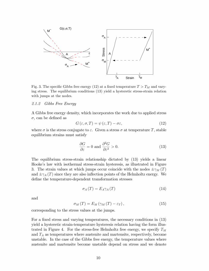
Fig. 3. The specific Gibbs free energy (12) at a fixed temperature T > TM and vary-ing stress. The equilibrium conditions (13) yield a hysteretic stress-strain relationwith jumps at the nodes.

2.1.2 Gibbs Free Energy

A Gibbs free energy density, which incorporates the work due to applied stressσ, can be defined as

G (ε, σ, T ) = ψ (ε, T )− σε, (12)

where σ is the stress conjugate to ε. Given a stress σ at temperature T , stableequilibrium strains must satisfy

∂G

∂ε= 0 and

∂2G

∂ε2> 0. (13)

The equilibrium stress-strain relationship dictated by (13) yields a linearHooke’s law with isothermal stress-strain hysteresis, as illustrated in Figure3. The strain values at which jumps occur coincide with the nodes ±γM (T )and ±γA (T ) since they are also inflection points of the Helmholtz energy. Wedefine the temperature-dependent transformation stresses

σA (T ) = EAγA (T ) (14)

andσM (T ) = EM (γM (T )− εT ) , (15)

corresponding to the stress values at the jumps.

For a fixed stress and varying temperatures, the necessary conditions in (13)yield a hysteretic strain-temperature hysteresis relation having the form illus-trated in Figure 4. For the stress-free Helmholtz free energy, we specify TMand TA as temperatures where austenite and martensite, respectively, becomeunstable. In the case of the Gibbs free energy, the temperature values whereaustenite and martensite become unstable depend on stress and we denote

10

Temperature

Str

ain

G(ε,σ,T)

ε

σ/EM

+εT

TMσ

M+

A

M+

A

σ/EA

M−

TAσ

TMσ

TAσ

Fig. 4. The specific Gibbs free energy (12) at a fixed stress and varying temperatures.The equilibrium conditions (13) yield a hysteretic strain-temperature relation withjumps at the stress-dependent transformation temperatures T σ

M and TσA.

them by T σM and T σ

A. After describing the chemical free energy in the nextsection, we derive relations for σA, σM , T σ

M , and T σA.

2.1.3 Chemical Free Energy

In a manner similar to that employed in [5,31,68,94,96], we model the chemicalfree energies as

βα (T ) =Z T

TRcαdT + uα − Tsa

= cα (T − TR) + uα − Tsα, (16)

where cα are specific heat capacities, which we assume to be explicitly temperature-independent. The constants uα denote the internal energies at reference tem-perature TR, and the sα are specific entropies of the form

sα =Z T

TR

cαTdT + ηα

= cα lnµT

TR

¶+ ηα, (17)

where ηα are the constant entropies at TR. The difference in the chemicalpotentials with a common reference temperature simplifies to

∆β (T ) = ∆u−∆ηT +∆c∙T − TR − T ln

µT

TR

¶¸, (18)

where∆u = uA−uM ,∆η = ηA−ηM , and∆c = cA−cM . As done in [41,68,71],we choose the reference temperature to coincide with the equilibrium temper-

11

ature Teq where ∆β (Teq) = 0. Therefore,

∆β (TR) = ∆u−∆ηTR

= ∆u−∆ηTeq = 0.

This then implies that, TR = Teq = ∆u/∆η. We specify that Teq satisfies theconditions Teq > 0 and TM < Teq < TA. Therefore, ∆u and ∆η are nonzeroand do not differ in sign for TR = Teq.

We now show that ∆u,∆η > 0. We first note that

∂∆β

∂T= −∆s

= −∆c ln

ÃT

Teq

!−∆η. (19)

Suppose ∆η < 0. If ∆c ≤ 0, then ∂∆β∂T

> 0 and ∆β (T ) > 0 for all T > Teq.However, as discussed in Section 2.1.1, we require ∆β (TA) < 0. Hence, ∆ηmust be positive when ∆c ≤ 0.

If ∆c > 0, then ∂∆β∂T

> 0 and ∆β (T ) < 0 for all positive T < Teq. However,we require ∆β (TM) > 0. So, ∆η must be positive when ∆c > 0. Therefore,we have ∆u > 0 and ∆η > 0.

The phase-dependent specific heat capacity of SMAs is not well-understoodand measured values vary greatly. Both positive and negative values of ∆chave been measured [26,41,69] and some SMA models assume that ∆c = 0with little or no experimental evidence [68,94]. The assumption that∆c = 0 isequivalent to making a first order Taylor approximation to (18) about T = TRsince

∆β (T ) = ∆u−∆ηT − ∆cTR2!

(T/TR − 1)2 +O³(T/TR − 1)3

´. (20)

Of course, the first-order truncation is a good approximation in cases wheretemperatures vary only in a neighborhood of TR and when ∆c ≈ 0.

We can write (18) in the non-dimensional form

b (θ) = 1− θ + a [θ − 1− θ ln (θ)] , (21)

where b (θ) = ∆β (T ) /∆u, θ = T/Teq, and a = ∆c/∆η. Figure 5 illustrates(21) for a ≥ 0.

As discussed in Section 2.1.1, for (18) to be consistent with (10) at tempera-tures below TM , we require∆β (T ) ≤ EMε2T/2. This condition can be satisfiedfor all T only when a ≥ 0. For a > 0, b (θ) is concave with a single maximum

12

0 0.25 0.5 0.75 1 1.25 1.5

−0.6

−0.4

−0.2

0

0.2

0.4

0.6

0.8

1

θ

b(θ)

a=2

a=1

a=1/2

a=1/4

a=0

a=0

a=2

Fig. 5. The non-dimensional chemical free energy (21) for various ∆c ≥ 0(a = 0, 1/4, 1/2, 1, 2). The general first-order approximation corresponds to the∆c = 0 (a = 0) case.

bmax at θ = e−1/a. Therefore,

bmax = 1 + a³e−

1a − 1

´≤ 12

EMε2T∆u

. (22)

Also, we note that while for all values of a there exists a zero at θ = 1, fora ≥ 1 there exists a second zero that does not correspond to a martensite-austenite equilibrium temperature (see Figure 5). Therefore, combining (22)with a < 1, we establish the condition

e−1 < 1− a³1− e−

1a

´≤ 12

EMε2T∆u

(23)

on the chemical free energy parameters to remain consistent with our definitionof the Helmholtz free energy at low temperatures. If energy parameters aresuch that (23) is violated (e.g., measured ∆c < 0), we enforce consistencyby setting ∆β (T ) = EMε2T/2 for all T < TM where ∆β (T ) > EMε2T/2 andsetting ∆β (T ) = 0 for all T < TM where ∆β (T ) < 0.

2.1.4 Local Transformation Stresses and Temperatures

Having specified the chemical free energy∆β (T ) in (18), we wish to determinethe explicit temperature-dependence of the local transformation stresses (14)and (15). Expressions for the transformation stresses in SMAs typically aredetermined from an approximation of a modified Clausius-Clapeyron equation,

13

which describes the effect of hydrostatic pressure on transformation temper-atures in a thermodynamic system [1,41,71,82,103]. However, we can obtainthe expressions directly from (6) and (11).

For T ≥ TM , (6) is underdetermined given only ∆β (T ). As an additionalconstraint we introduce

δ = σA (T )− σM (T ) , (24)

where δ is a material-dependent energy density that characterizes the hystere-sis size [94]. In general, δ is temperature-dependent, as observed in [41,71,95].In our present treatment, we approximate δ as a constant and we introducean implicit temperature-dependence in Section 2.4.

It follows from the construction of the Gibbs potential that σA (T ) > σM (T )for T ≥ TM . Furthermore, γM (T ) ≥ 0 in (15) for all T from which it followsthat δ ∈ (0, EMεT ]. With (24), we can formulate (6) solely in terms of σA (T ).This yields

F (σA (T )) =δεT2−∆β (T ) , (25)

where

F (σ) = σ

"εT +

(1−Er)

2EM(σ − δ)

#, (26)

and Er = EM/EA is less than one for shape memory compounds. Solving(25) for σA (T ) and recalling that σA (T ) ≥ 0 yields

σA (T ) =δ

2− EM

1−ErεT +

sδ2

4+

EM

1−Er

µEM

1−Erε2T − 2∆β (T )

¶. (27)

Note that the radicand in (27) is guaranteed to be non-negative provided

∆β (T ) ≤ 1

1−Er

EMε2T2

+1−Er

EM

δ2

8. (28)

Since (1−Er)−1 > 1 and we enforce ∆β (T ) ≤ EMε2T/2, (28) always holds.

The expression for σM (T ), when T ≥ TM , follows from (24) and (27). ForT < TM , (11) yields

σM (T ) = − 2εT

∆β (T ) . (29)

In this case, σM (T ) corresponds to the critical detwinning stress to the M−

variant.

We can also derive relations for the transformation temperatures. The stress-free transformation temperature TM satisfies

∆β (TM) =δεT2

(30)

14

since σA (TM) = 0. Furthermore, at TA where martensite becomes unstable,γM (TA) = εT . Hence,

∆β (TA) = −δεT2

. (31)

Under a nonzero stress σ, a transformation from austenite to martensite occurswhen σA (T

σM) = σ. In addition, σM (T σ

A) = 0 holds. Therefore, the stress-dependent transformation temperatures satisfy

∆β (T σM) =

δεT2− F (σ) (32)

and

∆β (T σA) =

δεT2− F (σ + δ) , (33)

whose solutions represent the inverses to σA (T ) and σM (T ), respectively. For∆c 6= 0, (30)—(33) must be solved numerically.

Figure 6 illustrates the relationship between the transformation stresses andtemperatures for a = 0, 1 and nominal values of the material constants. Thetemperature-dependent austenite-to-martensite critical stress σA correspondsto the stress-dependent austenite-to-martensite transformation temperatureT σM . Similarly, the martensite-to-austenite unloading stress σM for tempera-tures T ≥ TA corresponds to T σ

A. For T < TA, −σM (T ) is the critical detwin-ning stress. The plateau exhibited by the critical stress for low temperaturesis a result of enforcing ∆β (T ) ≤ EMε2T/2 and corresponds to γM (T ) = 0.

0.8 0.9 1 1.1 1.2 1.3 1.4 1.50

200

400

600

800

1000

1200

Normalized Transfomation Temperature (K/K)

Tra

nsf

orm

atio

n S

tre

ss (

MP

a)

σA(T)

σM

(T)

θA

θM

M+ Detwinning

Fig. 6. The phase transformation stresses and transformation temperatures normal-ized by Teq with θM = TM/Teq and θA = TA/Teq. The dashed lines are for a = 1and the solid lines are for a = 0.

15

2.2 Phase Evolution

Based on the local free energy, we follow the approach in [3,94] and model thephase evolution with the rate laws

x− (t) = PA−xA (t)− P−x− (t)

xA (t) = P−x− (t)− PA−xA (t) + P+x+ (t)− PA+xA (t) (34)

x+ (t) = PA+xA (t)− P+x+ (t) ,

where . denotes differentiation in time. The functions P± = P± (σ, T ) denotethe transition rates for M± lattice elements (transforming to either austeniteor a martensite variant), while PA± = PA± (σ, T ) denote the transition ratesfor austenite transforming to M±. Using the conservation relation (1), therate law reduces to

x− (t) = − (P− + PA−)x− (t)− PA−x+ (t) + PA−

x+ (t) = − (P+ + PA+)x+ (t)− PA+x− (t) + PA+. (35)

For the case T ≤ TM , the rate law for martensite variants simplifies to a singleODE

x+ (t) = − (P+ + P−)x+ (t) + P−, (36)

since x− (t) + x+ (t) = 1.

2.3 Transition Rates

We formulate the transition rates using the classical transition state theory ofnonequilibrium processes [36,86]. The theory stipulates that, due to thermalexcitation, lattice particles vibrate about equilibrium positions in energy wells.Furthermore, it contends that the vibrations are manifested as a temperature-dependent probability that the particles can overcome energy barriers sepa-rating the wells. For example, in the case of the local equilibrium conditions(13), the theory implies that thermally excited layers can transform from Ato M+ even when σA and T σ

M are not reached.

Transition state theory quantifies the transition rate by combining the likeli-hood that a particle will overcome a barrier with the frequency of attempts aparticle makes to overcome a barrier. The theory derives the likelihood thata lattice element will attain specific energy G using the Boltzmann relation

µ (G) = Ce−GV/kBT , (37)

where C is a normalization factor chosen to yield a likelihood of one whenintegrating µ (G) over all admissible energy states. The parameter kB =

16

1.380658 × 10−23 JK−1 is the Boltzmann constant and we assume the repre-sentative layer volume V is constant. We compute the transition rate for amartensite layer by multiplying (37) with the attempt frequency [86] to yield

P± (σ, T ) =

skBT

2πmV 2/3

e−G(±γM ,σ,T )V/kBTR±∞±γM e−G(γ,σ,T )V/kBTdγ

(38)

given a stress σ and temperature T , where m is the mass of the layer andG (±γM , σ, T ) is the Gibbs potential (12) at nodes ±γM (T ). In transitionstate theory, G (±γM , σ, T ) is termed the activation energy. Note that we setthe integration limits for the normalization factor to cover all possible stable(or metastable) martensite equilibrium states, neglecting the unstable statesdefined by the concave parabolae in (4). Likewise, the transition rate for anaustenite layer (T > TM) is given by

PA± (σ, T ) =

skBT

2πmV 2/3

e−G(±γA,σ,T )V/kBTR γA−γA e

−G(γ,σ,T )V/kBTdγ. (39)

Using (14), (15), and (25), we simplify the normalization integrals into tran-scendental functions of transformation stresses. This yields

P± (σ, T ) =1

τ

√Er

erfcxh(σM ∓ σ) /

√2ωM

i , (40)

whereerfcx (y) = ey

2

(1− erf (y)) (41)

is the scaled complementary error function and erf (y) = 2/√πR y0 e

−r2dr is thestandard error function. It then follows that PA± can be expressed as

PA± (σ, T ) =1

τ

n± erfcx

h(σ ∓ σA) /

√2ωA

i∓e∓2σAσ/ωA2 erfcx

h(σ ± σA) /

√2ωA

io−1. (42)

For T ≤ TM , where γA (T ) = 0, there is at most one energy state, so we definePA± (σ, T ) ≡ τ−1. The quantity

τ = π

sm

EAV 1/3(43)

represents a transformation relaxation time and the functions

ωα (T ) =

sEα

kBT

V(44)

quantify thermal energy densities for martensite and austenite.

17

Asymptotic analysis in [4] shows that erfcx (x) ≈ (√πx)−1 for large positivearguments and it is unbounded as x→−∞. Therefore, limσ→±∞ P± (σ, T ) =0 and limσ→±∞ PA± (σ, T ) =∞. Furthermore, at fixed temperatures

limωM→0

P± (σ, T ) =

⎧⎪⎪⎪⎪⎪⎨⎪⎪⎪⎪⎪⎩0 ±σ > σM (T )

τ−1√Er ±σ = σM (T )

∞ ±σ < σM (T )

(45)

and

limωA→0

PA± (σ, T ) =

⎧⎪⎪⎪⎪⎪⎨⎪⎪⎪⎪⎪⎩0 ±σ < σA (T )

τ−1 ±σ = σA (T )

∞ ±σ > σA (T ) .

(46)

The unbounded limits are a result of our mathematical description of theBoltzmann likelihoods. Physically, the unboundedness implies that a trans-formation will necessarily occur at precise thresholds of stress and temper-ature. Therefore, for small relative thermal energy (large volume V andno relaxation), the transformation behavior is governed by the deterministicequilibrium conditions (13). Otherwise, the stochastic transition rates implythat transformations can occur even when (13) do not hold. Furthermore,limωM→∞ P± (σ, T ) = τ−1

√Er (Boltzmann likelihood of one), which is the

value for σ = ±σM (T ), and limωA→∞ PA± (σ, T ) = ∞. When implementing(40) and (42), we define maximum likelihoods to occur at the transformationstresses, which implies that

P± (σ, T ) =

⎧⎪⎨⎪⎩τ−1√Er ±σ ≤ σM (T )

τ−1√Er

erfcx[(σM∓σ)/√2ωM ]

±σ > σM (T ) .(47)

Likewise, for T ≥ TM and |σ| < σA, (42) holds. Otherwise, we have that

PA± (σ, T ) =

⎧⎪⎨⎪⎩τ−1 T < TM

τ−1

erf[√2σA/ωA]

±σ ≥ σA (T ) .(48)

Note that (48) is unbounded, since

limT→TM+

PA± (±σA, T ) =∞. (49)

For this case, we heuristically assign a maximum greater than or equal toτ−1. Figure 7 illustrates (47) and (48) for small thermal energy in stress-temperature space.

18

P−(σ,T)

P+(σ,T)

0

PA−

(σ,T)

0

PA+

(σ,T)

TM

TM

TM

TM

σM

(TM

)

−σM

(TM

)

Temperature

Str

ess

P−= 0

P−= τ−1E

r1/2

P+= τ−1E

r1/2

P+= 0

PA+

= τ−1

PA+

= 0

PA−

= 0

PA+

= 1

σA(T)

σA(T)

−σM

(T)

σM

(T)

Fig. 7. The transition rates P± and PA± for varying temperature and stress at lowthermal energy. The solid lines mark the transformation boundaries defined bytransformation stresses and temperatures.

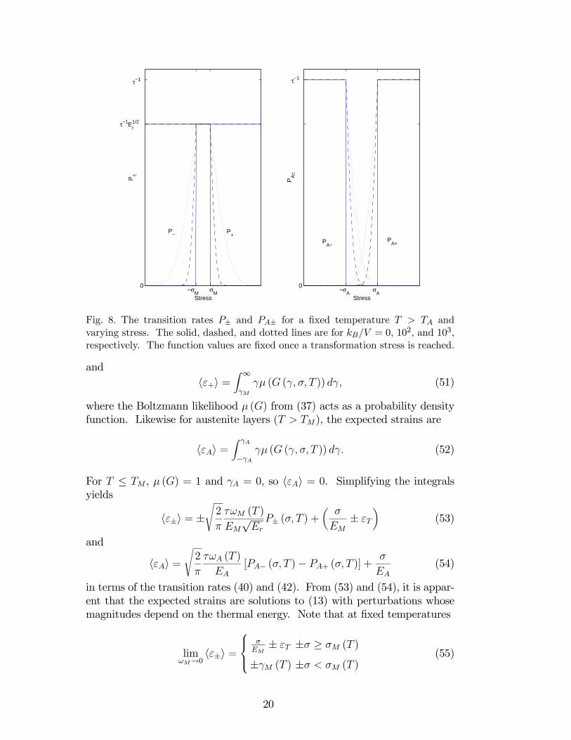
Ultimately, both (40) and (42) have qualities similar to those of a normal dis-tribution about σ, where the transformation stresses σα act as means and ωα asstandard deviations. Increasing thermal energy densities (large variances) in-creases the likelihood that transformations will occur when (13) do not hold.Diminishing thermal energy densities (small variances) restrict transforma-tions to occur only when (13) are satisfied. Figure 8 illustrates the transitionrates for increasing ωα at a fixed temperature and decreasing activation vol-umes.

2.4 Expected Local Strains

Given the temperature evolution T (t) and the phase fractions modeled by(35), we can now quantify the thermomechanical response of the material.Boltzmann statistics govern the response of individual martensite and austen-ite layers. Accounting for thermal energy, the expected strain exhibited bymartensite layers are given by

hε−i =Z −γM−∞

γµ (G (γ, σ, T )) dγ (50)

19

0

StressP

A±

0

Stress

P±

σM

−σM

σA

−σA

τ−1Er1/2

τ−1 τ−1

P+ P

−

PA+P

A−

Fig. 8. The transition rates P± and PA± for a fixed temperature T > TA andvarying stress. The solid, dashed, and dotted lines are for kB/V = 0, 102, and 103,respectively. The function values are fixed once a transformation stress is reached.

andhε+i =

Z ∞γM

γµ (G (γ, σ, T )) dγ, (51)

where the Boltzmann likelihood µ (G) from (37) acts as a probability densityfunction. Likewise for austenite layers (T > TM), the expected strains are

hεAi =Z γA

−γAγµ (G (γ, σ, T )) dγ. (52)

For T ≤ TM , µ (G) = 1 and γA = 0, so hεAi = 0. Simplifying the integralsyields

hε±i = ±s2

π

τωM (T )

EM

√Er

P± (σ, T ) +µ

σ

EM± εT

¶(53)

and

hεAi =s2

π

τωA (T )

EA[PA− (σ, T )− PA+ (σ, T )] +

σ

EA(54)

in terms of the transition rates (40) and (42). From (53) and (54), it is appar-ent that the expected strains are solutions to (13) with perturbations whosemagnitudes depend on the thermal energy. Note that at fixed temperatures

limωM→0

hε±i =⎧⎪⎨⎪⎩

σEM

± εT ±σ ≥ σM (T )

±γM (T ) ±σ < σM (T )(55)

20

0

Temperature

0

0

Stress

Stra

in

TMσ T

Aσ T

MT

A−σ

A −σ

Mσ

Mσ

A

γM

γA

−γA

−γM

σ/EA

σ/EM

+eT

σ/EM

−eT

<ε+>

<εA>

<ε−>

<ε+>

<εA>

<ε−>

Fig. 9. The expectation strains (53) and (54) as a function of stress (T > TA) andtemperature for low thermal energy.

and

limωA→0T>TM

hεAi =⎧⎪⎨⎪⎩

σEA

|σ| ≤ σA (T )

±γA (T ) ±σ > σA (T ) .(56)

Furthermore, limσ→∓∞ hε±i = ±γM and limσ→±∞ hεAi = ±γA. Figure 9 illus-trates the stress and temperature-dependence of (53) and (54).

With the expected strain of a layer in each phase thus formulated, the averagelocal strain can be expressed as the weighted sum

εmech =Xα

xα hεαi . (57)

In addition to the strain εmech attributed to mechanical deformation and phasetransformation processes, there are strains due to local thermal expansion asthe temperature varies over time. We model the local thermal strain as

εther = λ (xα) (T − T0) (58)

for the phase-dependent thermal expansion coefficient λ (xα) =P

α λαxα (t),and initial temperature T0. Therefore, the total average strain of a layer inresponse to a combination of applied stress and temperature is

ε = εmech + εther. (59)

Typically, εther is negligible compared to εmech for moderate temperaturechanges as would be encountered in bulk superelastic applications. How-

21

0 0

Strain

Str

ess

0

Str

ain

Temperature

σA

σM

γA γ

M

kB/V = 102

kB/V = 0

kB/V = 10

M+

A

A

M+

σ/EA

σ/EM

+εT k

B/V = 0

TM

TA

kB/V = 102

Fig. 10. Superelasticity (fixed T > TA) and shape memory effect (fixed stress)hysteresis determined from (57). The largest hysteresis loops occur for kB/V = 0and hysteresis diminishes to zero for increasing kB/V .

ever for thin films in MEMS applications, thermal strains can have significanteffects on microdevice behavior (e.g., see [49,79]).

Figure 10 illustrates stress-strain (superelastic) and temperature-strain (SME)hysteresis predicted by (57). For diminishing thermal energy, hysteresis in-creases to a maximum and corresponds to the equilibrium solution (13). Forincreasing thermal energy densities, more lattice layers overcome energy bar-riers before transformation thresholds are reached, resulting in a smaller hys-teresis loops. If the thermal energy is sufficiently large, all energy barriersbecome surpassable at any stress and temperature. In this case, layers attainthe global minimum of (12) and there is no hysteresis. We note that the di-minishing hysteresis reflects an implicit temperature-dependence of δ in (24),where ∂δ

∂T< 0 provided limT→∞ σα (T ) /ωα (T ) = 0.

In the next section, we model the variation of temperature over time due tophase transformations and ambient conditions.

2.5 Thermal Evolution

The internal temperature of an SMA is coupled to the thermomechanical phasetransformations and it strongly depends on operating conditions. We describetemperature changes in the material via a simplified balance of internal energy,

22

similar to the developments in [14,26,94]. In this case,

c (xα) T (t) = −Xα

hαxα +H (xα, T ) , (60)

where c (xα) =P

α cαxα (t) represents a linear mixture of phase-dependent spe-cific heats. In the following subsections, we describe the components formingthe right-hand-side of (60), which include transformation-induced heat gener-ation and heat exchange with the environment.

2.5.1 Transformation Enthalpy

The first term on the right-hand side of (60) accounts for rate-dependent heatgeneration and absorption during phase transformations. The release andabsorption of transformation enthalpies can be significant and is a source ofthe material self-heating observed in [95]. The specific enthalpies hα have theform

hα = gα + Tsα. (61)

In (61), gα is a local minimum of (12) and sα is the specific entropy from (17).Given stress σ at temperature T ,

gA =−σ22EA

+∆β (T ) (62)

g± =−σ22EM

∓ σεT . (63)

SinceP

α xα (t) ≡ 0, we haveXα

hαxα = − (hA − h−) x− − (hA − h+) x+, (64)

and

hA − h± =σ2

2

µ1

EM− 1

EA

¶± σεT +∆c (T − TR) +∆u. (65)

The differences in martensite and austenite specific enthalpies in (65) arereferred to as latent heats of transformation. Note that for T ≤ TM , (64)reduces to X

α

hαxα = −2σεT x+. (66)

2.5.2 Heat Transfer

Heat transfer is a phenomenon pertaining to a physical system of which anSMA is a component, rather than a constitutive property of the material.However, for basic actuator simulations and model comparisons to thermo-mechanical tests, we introduce the thermal interaction of the material with

23

its environment via H (xα, T ) in equation (60). For our uniaxial model, weassume that the temperature is spatially uniform in SMAs such as thin filmsand wires. A uniform longitudinal temperature distribution can be realized ina thermal chamber or in transducers with resistive heating. Additionally weassume that internal temperature can be approximated effectively by modelsof heat transfer at the surface. We establish the validity of this assumptionby calculating the dimensionless Biot number Bi (see [27,47,69,96]) given by

Bi =hckαΩ

, (67)

where hc is the phenomenological average convection heat transfer coefficient,kα is the phase-dependent thermal conductivity, and Ω is the surface area-to-volume ratio. For Bi ¿ 1, the temperature changes within the materialare negligible relative to temperature differences between the surface and sur-roundings [47]. For SMAs such as NiTi, the conductivity kα is on the orderof 10 Wm−1K−1 and hc is on the order of 1 and 102 Wm−2K−1, depending onambient flow conditions [14,69]. Furthermore, for rectangular geometries ofthickness d, width w and length L,

Ω = 2µ1

d+1

w+1

L

¶. (68)

Likewise, for cylindrical geometries of diameter d,

Ω = 2µ2

d+1

L

¶. (69)

Hence, for thin films and wires where d ¿ L,w, Ω is O (d−1) and Bi isO (10m−1 d). In the applications under consideration, SMA thicknesses areat most 1 mm, so Bi¿ 1 is satisfied.

Incorporating surface convection and radiation, and resistive Joule heating,the term H in (60) can be expressed as

H (xα, T ) = − (hc + hr)Ω [T (t)− TE (t)] + J (xα, T ) , (70)

where TE (t) is the prescribed external temperature. The radiation heat trans-fer coefficient is given by

hr = σB³T 2 + T 2E

´(T + TE) ,

where ∈ [0, 1] is the surface emissivity (. 0.50 for metals, . 0.20 for films)and σB = 5.67051×10−8Wm−2K−4 is the Stefan-Boltzmann constant. In gen-eral, hc is also (weakly) temperature-dependent and is estimated from empiri-cal arguments involving surface geometry and external fluid flow. In our treat-ment, we assume hc is constant and we refer the reader to [14,27,47,55,69,85,87]for theoretical and empirical aspects of hc pertinent to SMAs. Note that in

24

forced convection conditions, hc is typically one to three orders of magnitudegreater than hr over all temperatures.

Lastly, in (70), J (xα, T ) incorporates heat generation via resistive Joule heat-ing. For current-controlled applications,

J (xα, T ) = ρe (xα, T )I2

ζ2, (71)

where I is the applied current and ζ is the cross sectional area of the currentpath. The effective resistivity

ρe (xα, T ) =Xα

(ρeα + λeαT )xα (t) (72)

includes the phase-dependent electrical resistivities ρeα, and linear tempera-ture coefficients of resistivity λeα. If Joule heating results from a prescribedpotential difference, we have

J (xα, T ) =1

ρe (xα, T )

V 2e

L2, (73)

where Ve is the applied voltage and L is the actuator length.

The temperature-dependence of resistivity can be significant when quantifyingresistivity-temperature hysteresis [106,111]. However, in cases where Jouleheating is an impulse heat source, as is typical for MEMS applications, theexplicit temperature-dependence is negligible.

In general, the geometric quantities Ω, ζ, and L are functions of uniaxial strain.For example, in a rectangular geometry Ω changes by a factor of (1− νε)−1,ζ by a factor of (1− νε)2, and L by a factor of (1 + ε), where the isotropicPoisson ratio ν ∈ [0, 0.5] (ν ≈ 0.33 for isochoric NiTi). Since typical actuatorstrains are at most on the order of 10%, the relation (70) can change on theorder of 5-15% due to deformations. To facilitate model computation, weapproximate Ω, ζ, and L as constants.

We have modeled the phase fractions, expected strains, and temperature withfree energy expressions that are valid for local lattice behavior. Equation(59) also quantifies macroscopic strains for specially-prepared homogeneous,single-crystal SMAs in which the bulk lattice exhibits uniform local behavior.In the next section, we extend our uniform lattice model to more generalinhomogeneous compounds, where the local thermomechanical behavior canvary throughout the material.

25

3 Nonuniform Lattice Model

Typical single-crystal and polycrystalline SMA compounds contain precipi-tates, dislocations, and process-induced impurities. Moreover, inhomogeneousand polycrystalline materials have a nonuniform lattice structure that inducesvariations in the local material response. In this section, we model the hystere-sis induced in nonuniform SMA lattices and the effects of nonuniform stressfields by employing a statistical homogenization technique. For a discussionof general statistical homogenization concepts, we refer the reader to [62,86].Our approach is based on the assumption that measurements of macroscopicphenomena, such as stress-strain hysteresis and transformation temperatures,yield quantities that reflect a distribution of local variations. In the contextof statistical homogenization, the uniform lattice model (59) predicts the ex-pected local response when given effective macroscopic material parametersas input.

3.1 Variations in Hysteresis

One approach to account for inhomogeneities is to treat measurements ofmacroscopic hysteresis parameters, such as εT and δ, as manifestations ofstochastic distributions, rather than deterministic values. In particular, vari-ations of δ and εT produce variations in the transformation thresholds σA, σM ,TM and TA via (27), (30), and (31), and they reflect variations in the chemicalfree energy parameters. We model the effects of varying δ on the observedmacroscopic strain ε by considering the statistical average

ε (σ, T ) =Z ∞0

ε (σ, T ; δ) p1 (δ) dδ, (74)

where ε is the local strain in (59), and p1 is a probability density functiondefined on [0,∞). Reflecting the boundedness of δ, we represent p1 as a log-normal distribution on the interval (0, EMεT ], given EM and εT .

As detailed in [72], the normalized log-normal probability density function isgiven by

p1 (δ) =1

z√2πδ

e− ln(δ/µ)2/2z2 (75)

with parameters z > 0 and µ > 0. As illustrated in Figure 11, the log-normal distribution is continuous and right-skewed, and the logarithm of thedistributed variable has a normal distribution. Increasing z and µ correspondto increasing skewness. In cases where mean δ and standard deviation zδ ofδ are given (e.g., experimental estimates), the log-normal parameters can becomputed via the relations

µ = δ

Ãz2δδ2+ 1

!− 12

, z2 = ln

Ãz2δδ2+ 1

!. (76)

26

0 0

Distributed Variable

Pro

babi

lity

Den

sity

Log−normalNormal

µ µ^

Fig. 11. The log-normal probability density function compared with its normal coun-terpart. The peak of the skewed log-normal function corresponds with the modeand the peak of the normal curve corresponds with the mean µ. The areas underthe curves correspond to the same probability.

3.2 Effective Stress

In addition to the model (74) which incorporates material inhomogeneities,we quantify the effects of nonuniform stress fields. We represent the localeffective stress σe as a perturbation of the macroscopic applied stress

σe (t) = σ (t) + s, (77)

where σ is the time-varying applied stress and s is a constant perturbation,which we assume to be a random variable. The observed macroscopic strainis then a response to a distribution of effective stresses in the material

ε (σ, T ) =Z ∞−∞

ε (σe, T ) p2 (s) ds, (78)

where p2 is a probability density function defined on (−∞,∞). We assume s isnormally distributed, so we take p2 to correspond with the normal distribution

p2 (s) =1√2πzσ

e−s2/2z2σ (79)

27

with standard deviation zσ. For certain geometries and load conditions, onecan alternatively employ the trigonometric averaging procedure proposed in[83] to accommodate stress variations on rotated polycrystal grains. In par-ticular, by distributing about the applied stress, we account for polycrystalgrains undergoing stress and temperature-induced transformations at varyingapplied stresses and temperatures.

3.3 Macroscopic Model

The combination of (74) and (78) yields the relation

ε (σ, T ) =Z ∞0

Z ∞−∞

ε (σe, T ; δ) p1 (δ) p2 (s) dsdδ (80)

for the total macroscopic response to a time-varying stress σ (t) and an evolv-ing internal temperature T (t). In addition to the measured strain, the macro-scopic phase fractions xα and internal temperature T are also representationsof the underlying distributions. We compute these macroscopic quantitiesby replacing ε with xα and T in (80). Table 1 summarizes the parametersused in the local and macroscopic models. In the next section, we discussimplementation issues associated with the macroscopic model (80).

4 Numerical Implementation and Simulations

4.1 Implementation

In this section, we summarize aspects of the numerical implementation of themacroscopic model. To obtain the macroscopic strain response given a time-varying stress, environment temperature, and current or voltage, we solve thelocal model over distributed δ and σe in (80). At the core of the local modelis the nonlinear system of ODEs for the phase fractions and temperature. Weexpress the system as⎡⎢⎣ x− (t)x+ (t)

T (t)

⎤⎥⎦ =M (xα, T )

⎡⎢⎣x− (t)x+ (t)T (t)

⎤⎥⎦+⎡⎢⎣PA− (σ, T )PA+ (σ, T )H (xα, T )

⎤⎥⎦ , (81)

where the state-dependent matrixM is given by

M (xα, T ) =

⎡⎢⎣ 1 0 00 1 0

LA−c(xα)

LA+c(xα)

1c(xα)

⎤⎥⎦⎡⎢⎣− (P− + PA−) −PA− 0

−PA+ − (P+ + PA+) 00 0 1

⎤⎥⎦and LA± = hA − h±. Recall that the latent heats and the transition ratesdepend on stress and temperature. The first step in solving the local model is

28

Parameter Physical Description

Physical Parameters

EA, EM Elastic moduli (linear).

λA, λM Thermal expansion coefficients (linear).

cA, cM Volumetric specific heat capacities (ρcV ).

∆u Specific internal energy difference at reference.

∆η Specific entropy difference at reference.

V Activation volume (local).

τ Transformation relaxation time.

Hysteresis Parameters

εT Transformation strain.

δ, zδ Mean hysteresis thickness and standard deviation.

zσ Effective stress standard deviation.

Heat Transfer ParametersρeA, ρ

eM Resistivities.

λeA, λeM Temperature coefficients of resistivity.

Surface emissivity.

hc Convective heat transfer coefficient.

Geometric ParametersL, d,w Length, thickness (or diameter), width.

Table 1. Local and macroscopic model parameters.

to obtain initial data x± (0) and T (0) from experimental conditions. Typicalinitial conditions are the high-temperature state where x± (0) = 0 or theunstressed low temperature (self-accommodating) state where x± (0) = 1/2.Secondly, we calculate necessary model parameter estimates, as described inthe next section, from given material data, such as the distributed value of δ.Next, we solve (81) using the Matlab ODE routine ode15s, which is a variableorder solver based on the numerical differentiation formulas. To compute theintegrals in the transition rates and the expectation strains, we utilize theMatlab routines erf and erfcx, which approximate the functions directly withpolynomials. Finally, we compute the thermal strains and total local straingiven the expectation strains and the ODE solution.

To integrate the macroscopic model, we approximate the distribution inte-grals with composite Gauss-Legendre quadrature on finite intervals. Here wehave adapted the scalar, univariate formulation described in [61] to the caseof vector-valued functions. For scalar argument x we define the vector-valuedfunction f (x) ∈ <1×m. The n-point composite Gauss quadrature approxi-

29

mates the component-wise integral F ∈ <1×m on interval [ax, bx],

F =Z bx

axf (x) dx

≈ bx − ax2kx

c|kxXj=1

fj (82)

for kx uniform subintervals of [ax, bx], with n quadrature points in each subin-terval. The vector of quadrature weights c ∈ <n×1 is given by

c = [c1, c2, · · · , cn]| . (83)

At the jth subinterval, we define fj ∈ <n×m as

fj =hf (x1,j) , f (x2,j) , · · · , f (xn,j)

i|, (84)

where the nodes

xij = ax +bx − ax2kx

(xi + 2j − 1) , i = 1 : n, j = 1 : kx (85)

are mapped from tabulated Gauss nodes xi on the standard interval [−1, 1].For the full macroscopic model, we require double integration, so we employthe composite n-point quadrature rule iteratively on f as a function of scalarsx and y

F =Z by

ay

Z bx

axf (x, y) dxdy

≈Ãbx − ax2kx

!Ãby − ay2ky

! kyXjy=1

nXi=1

cic|

kxXjx=1

fjx,i,jy , (86)

where ky is the number of subintervals in [ay, by] and ci is the ith componentof c. The function fjx,i,jy ∈ <n×m is evaluated at the jthx x-subinterval and thejthy y-subinterval

fjx,i,jy =hf³x1,jx , y1,jy

´, f³x2,jx , y2,jy

´, · · · , f

³xn,jx, yn,jy

´i|. (87)

The y-nodes are given by

yij = ay +by − ay2ky

(xi + 2j − 1) , i = 1 : n, j = 1 : ky.

In our implementation, fjx,i,jy corresponds to the integrand of (80) where thelocal strain solution ε (σ + σe, T ; δ) is discretized over an interval of m timesteps. In addition, we take the finite integration intervals to correspond with

30

Nodes Weights

±√15−2√30√35

18+√30

36

±√15+2

√30√

3518−√3036

Table 2. Four-point Gaussian quadrature nodes and weights on [-1,1].

[µ− qz, µ+ qz], where µ is the arithmetic mean and qz is a multiple of thestandard deviation for each distribution. For q ≥ 2, the interval encompassesat least 95.4% of the probability. In our calculations, we use a four-pointquadrature rule having the standard nodes and weights listed in Table 2.Finally, we note that the quadrature solves (81) at [(n− 1) k + 1]2 nodes andthat the overall efficiency of the model algorithm primarily depends on therapid computation of ε.

4.2 Simulations

In this section, we demonstrate and analyze the material behavior predicted bythe model. Specifically, we illustrate superelasticity, the shape memory effect,and heat transfer phenomena pertinent to thin-film SMAs. Table 3 summa-rizes the default parameters used in this section’s simulations where we assumea rectangular SMA geometry. Additionally, we assume a material density ofρ = 6450 kg/m3, corresponding to published values of polycrystalline NiTiwires. Since we do not demonstrate temperature-resistivity hysteresis, we donot specify the temperature coefficients of resistivity λeA and λeM .

The mean local energy parameters∆u = 73.8MJ/m3,∆η = 0.218MJ/m3K−1

are estimated from (18) and (25) given the parameters in Table 3, σA (353 K) =212 MPa, and Teq = 338 K. In solving the macroscopic model, we recalculatethe estimates of ∆u and ∆η in this manner for each distributed value of δ.

4.2.1 Superelasticity

Figure 12 illustrates superelasticity predicted by the model. The initial stateis taken to be austenite at ambient temperature and a load is prescribed at arate of 1 MPa/s. In contrast to the abrupt transitions illustrated in Figure 12for the local material behavior, the macroscopic model predicts gradual andasymmetric transitions. In addition to a nonuniform lattice structure, theinternal temperature evolution is a source of the gradual transitions. Duringthe transformation from austenite to detwinned martensite, transformationenthalpy is released. Some of the heat is transferred to the environment viaconvection while the remainder produces an increase in the internal temper-ature as shown in Figure 12. Therefore, the temperature-dependent loading

31

Physical Value UnitsEA, EM 22.4, 13.7 GPaλA, λM 11.0, 6.6 10−6/KcA , cM 3.744, 2.903 MJ /m3K−1

V 6903 nm3

τ 1.1 ms

Heat TransferρeA, ρ

eM 100,80 µΩ cm

0.10hc 10 W /m2K−1

HysteresisεT 0.0248δ, zδ 152, 35 MPazσ 25 MPa

GeometricL 1.5 cmd 100 µmw 1.8 mm

Table 3. Mean local parameter values used by default in simulations. Changes fromthe default in particular simulations are noted in the text.

transformation stress increases during a transformation. The reverse processoccurs for the unloading stress.

Figure 13 illustrates the temperature-dependent stress-strain hysteresis pre-dicted by the model. We start with temperatures at which austenite is sta-ble. At cooler temperatures, self-accommodating martensite (50% M+, 50%M−) is the initial phase and the stress-induced transformation corresponds tomartensite detwinning. Agreeing with experimental observations in [42,50],the yield stress from austenite to martensite is shown to increase as tem-

0 200 400 600 800 1000364

366

368

370

372

Time (s)

Tem

pera

ture

(K

)

0 200 400 600 800 10000

0.5

1

Pha

se F

ract

ion

0.01 0.02 0.03 0.04 0.05 0.060

50

100

150

200

250

300

350

400

450

500

Strain

Str

ess

(MP

a)

A

M+

Fig. 12. Superelasticity at TE = 358 K. The release and absorption of transforma-tion enthalpies yield internal temperature changes.

32

0 0.02 0.04 0.06 0.080

100

200

300

400

500

600

700

800

900

Strain

Str

ess

(MP

a)

0 0.02 0.04 0.06 0.080

100

200

300

400

500

600

700

800

900

Strain

Str

ess

(MP

a)

408 K378 K348 K

315 K325 K338 K

Fig. 13. The temperature-dependence of the hysteresis. For T ≥ 348 K, austeniteis the initial phase. Self-accommodating martensite is the initial phase for lowertemperatures.

peratures increase, and the detwinning critical stress is shown to increase astemperatures decrease at lower temperatures. In Section 6.2, we compare themodel to experimental superelasticity data.

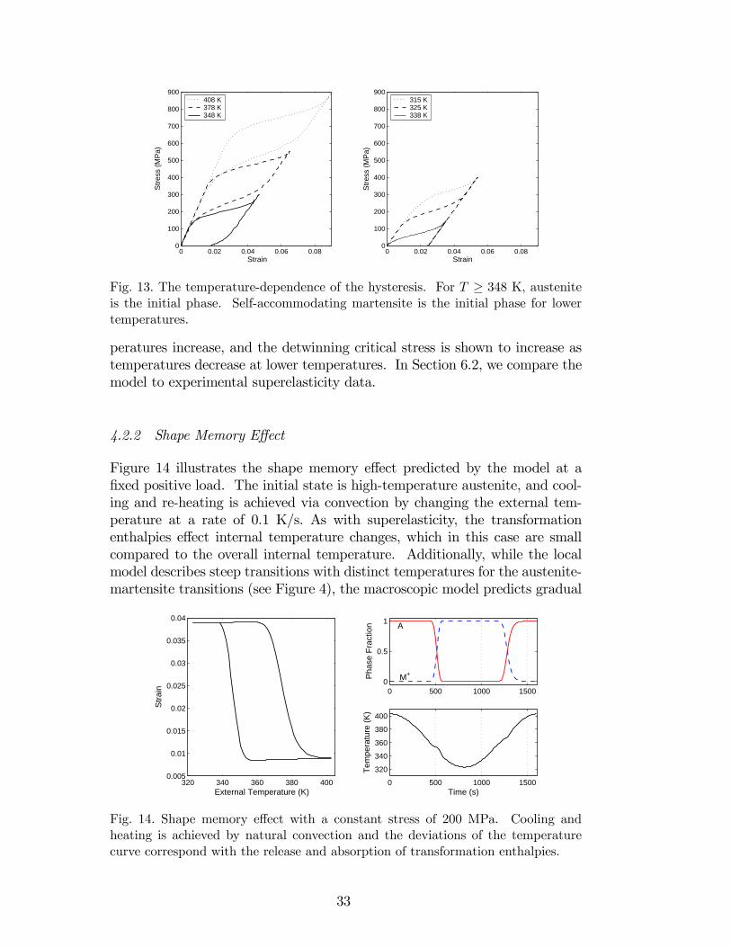
4.2.2 Shape Memory Effect

Figure 14 illustrates the shape memory effect predicted by the model at afixed positive load. The initial state is high-temperature austenite, and cool-ing and re-heating is achieved via convection by changing the external tem-perature at a rate of 0.1 K/s. As with superelasticity, the transformationenthalpies effect internal temperature changes, which in this case are smallcompared to the overall internal temperature. Additionally, while the localmodel describes steep transitions with distinct temperatures for the austenite-martensite transitions (see Figure 4), the macroscopic model predicts gradual

0 500 1000 1500

320

340

360

380

400

Time (s)

Tem

pera

ture

(K

)

0 500 1000 15000

0.5

1

Pha

se F

ract

ion

320 340 360 380 4000.005

0.01

0.015

0.02

0.025

0.03

0.035

0.04

External Temperature (K)

Str

ain

A

M+

Fig. 14. Shape memory effect with a constant stress of 200 MPa. Cooling andheating is achieved by natural convection and the deviations of the temperaturecurve correspond with the release and absorption of transformation enthalpies.

33

transitions where the beginning and end of the thermal transformations arenot distinctly defined.

Figure 15 illustrates the stress-dependence of thermal hysteresis predicted bythe model. The stress-dependent transformation temperatures are shown todecrease as stress decreases. Also, the transformation strain from austeniteto detwinned martensite is shown to decrease rapidly at lower stresses. Thisexperimentally verified behavior is attributed to the fact that low stresses areinsufficient to induce a uniform transformation throughout the material (e.g.,see [31,51]). The incorporation of effective stresses in (80) allows us to simulatethis phenomenon and we note that other models are unable to account for thisbehavior [15,31,88]. In Section 6.3, we compare experimental SME data tomodel predictions.

300 350 400 4500

0.005

0.01

0.015

0.02

0.03

0.035

0.04

0.045

0.05

External Temperature (K)

Str

ain

300 350 400 4500

0.005

0.01

0.015

0.02

0.03

0.035

0.04

0.045

0.05

External Temperature (K)

Str

ain

15 MPa35 MPa75 MPa

200 MPa275 MPa350 MPa

εT ε

T

Fig. 15. The stress-dependence of thermal hysteresis. The initial phase is austeniteat high temperatures and the low temperature phase is M+.

4.2.3 Heat Transfer Effects

Here we investigate heat transfer aspects of the model with examples pertain-ing to thin-film SMA behavior. From (68), we see that the surface area tovolume ratio of thin films is approximately d−1. Accordingly, the effects of heattransfer will be prominent for thin films, which are 2-3 orders of magnitudethinner than typical bulk SMA wires and bars.

Figure 16 illustrates how thickness affects hysteresis in our model. Increasedheat transfer due to increasing Ω allows latent heat to be quickly absorbedor released during transformations. Therefore, decreasing thicknesses yieldless hysteresis, which allow for full actuation at smaller changes in stress andtemperature.

In Figure 17, we demonstrate the actuation of a 10 µm thin-film SMA viaimpulse Joule heating and forced convective cooling (hc = 300Wm−2/K). TheSMA is in a 303 K environment under a fixed stress of 100 MPa. Under these

34

0 0.02 0.04 0.06 0.080

100

200

300

400

500

600

700

Strain

Str

ess

(MP

a)

300 320 340 360 380 400 4200.01

0.015

0.02

0.025

0.03

0.035

0.04

0.045

External Temperature (K)

Str

ain

Fig. 16. Superelasticity (TE = 358 K) and SME (250 MPa) for different film thick-nesses. The solid, dashed, and dotted curves are for d = 10, 100, and 1000 µm, re-spectively. The standard deviations are taken to be zσ = 20MPa and zδ = 20MPa.

conditions, the SMA is deformed 3.2% as detwinned martensite. We simulateda low voltage of 2 V for a duration of 10 ms, which increases the temperatureby 50 K and induces a partial transformation to austenite with 1.2% recoveredstrain. A second and third impulse heating separated by 21 ms cooling timesyields a full transformation to austenite and full deformation recovery. Finally,full reversion to martensite via forced convection is achieved in 50 ms. Theinner loop, which demonstrates that the model can maintain loop closure,corresponds to the first partial heating-cooling cycle.

From the temperature evolution in Figure 17, we conclude that cooling timein our model is the limiting factor for thin-film SMA actuator response. Wealso note the plateau in the temperature evolution. The delay in coolingcorresponds with the phase transformation and is due to the exchange oftransformation enthalpies. Similar analytical and experimental results are

300 320 340 360 380 4000

0.005

0.01

0.015

0.02

0.025

0.03

Internal Temperature (K)

Str

ain 0 0.05 0.1 0.15 0.2 0.25

0

0.5

1

Pha

se F

ract

ions

0 0.05 0.1 0.15 0.2 0.25300

350

400

Time (s)

Tem

pera

ture

(K

)

A

M+

Fig. 17. Joule heating of a thin-film SMA and cooling via forced convection. The10 µm film is under a 100 MPa stress and is initially detwinned martensite. Thestandard deviations are taken to be zσ = 35 MPa and zδ = 35 MPa.

35

reported in [69,87] and we note that [73] concludes that the response of thin-film SMA actuators is ultimately limited by the rate of phase transformationsrather than the cooling time.

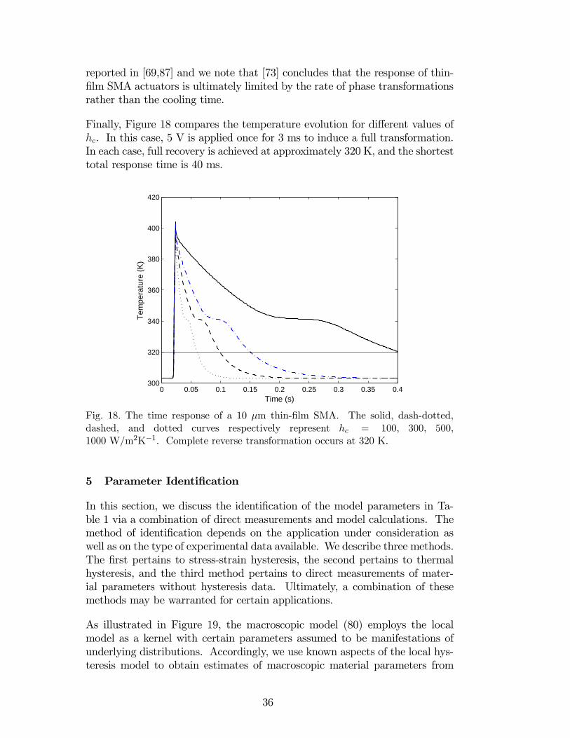
Finally, Figure 18 compares the temperature evolution for different values ofhc. In this case, 5 V is applied once for 3 ms to induce a full transformation.In each case, full recovery is achieved at approximately 320 K, and the shortesttotal response time is 40 ms.

0 0.05 0.1 0.15 0.2 0.25 0.3 0.35 0.4300

320

340

360

380

400

420

Time (s)

Tem

pera

ture

(K

)

Fig. 18. The time response of a 10 µm thin-film SMA. The solid, dash-dotted,dashed, and dotted curves respectively represent hc = 100, 300, 500,1000 W/m2K−1. Complete reverse transformation occurs at 320 K.

5 Parameter Identification

In this section, we discuss the identification of the model parameters in Ta-ble 1 via a combination of direct measurements and model calculations. Themethod of identification depends on the application under consideration aswell as on the type of experimental data available. We describe three methods.The first pertains to stress-strain hysteresis, the second pertains to thermalhysteresis, and the third method pertains to direct measurements of mater-ial parameters without hysteresis data. Ultimately, a combination of thesemethods may be warranted for certain applications.

As illustrated in Figure 19, the macroscopic model (80) employs the localmodel as a kernel with certain parameters assumed to be manifestations ofunderlying distributions. Accordingly, we use known aspects of the local hys-teresis model to obtain estimates of macroscopic material parameters from

36

320 340 360 380 4000.005

0.01

0.015

0.02

0.025

0.03

0.035

0.04

External Temperature (K)

Str

ain

0 0.01 0.02 0.03 0.04 0.050

50

100

150

200

250

300

350

400

Strain

Str

ess

(MP

a)

Fig. 19. The average local material response (solid) given by (59) compared withthe statistically homogenized macroscopic response (dashed) given by (80).

measured hysteresis data. Estimates of the mean local parameters in Table 1along with the distribution parameters, zδ and zσ provide us initial parametervalues for use in least squares fits to hysteresis data. We note that the acti-vation volume V and the relaxation time τ typically must be estimated fromhysteresis data.

5.1 Stress-strain Hysteresis

One or more experimental stress-strain hysteresis curves are sufficient to esti-mate most of the material parameters pertaining to superelasticity. As illus-trated in Figure 20, the elastic moduli can be estimated from linear portionsof the loading or unloading curves. In particular, EA should be measuredfrom linear portions of loading curves at sufficiently high temperatures. Simi-larly, EM can be measured from loading curves at relatively cool temperatures.Also at cool temperatures, εT can be measured as the residual strain after fulltransformation detwinning [68]. Alternatively, both EM and εT can be iden-tified simultaneously by extrapolating a line from the superelastic unloadingcurve as depicted in Figure 20. Furthermore, δ is estimated from the meanthickness of superelastic hysteresis.

With measurements of EA, EM , εT , and δ, the local relations (18), (25), (29),can be used to calculate the chemical free energy parameters ∆u, ∆η, and ∆c(recall TR = Teq = ∆u/∆η). In this case, we also require the measurement ofσA or σM at one or more temperatures as depicted in Figure 20. Therefore,if we make the first order approximation of ∆c = 0, only two stress-strainhysteresis curves at different temperatures are required to identify the localmodel fully for the prediction of superelasticity. Given the behavior illus-

37

0 0

Str

ess

StrainεT

σ/EM

+ εT

σ/EA

σA

1

σA

2

δ−

Fig. 20. Identification of material parameters using stress-strain hysteresis data. Thedashed hysteresis curve corresponds to the higher ambient temperature T2 > T1.

trated in Figure 19, we can estimate zδ and zσ from the loading and unloadingtransformation regions.

We note that we have neglected to take into account heat transfer and ratephenomena described in Section 4.2 and we have implicitly assumed that thethermal activation effects described in Section 2.4 are insignificant. We takethe identification methods we have described for near-isothermal, quasi-staticcases as a first approximation for these cases. Finally, thermal expansion isnormally negligible in superelasticity due to the small temperature changes.Nevertheless, the coefficients can be estimated using

λα =ε1 − ε2T1 − T2

, (88)

where εi are strains measured at the same stress level for temperatures Ti.

5.2 Thermal Hysteresis

Heat transfer effects are prominent in thermal hysteresis experiments; how-ever, these effects can be minimized by slow heating rates, high rates of heattransfer, or direct measurements of the internal SMA temperature. One ormore experimental temperature-strain hysteresis curves are sufficient to es-timate most of the material parameters pertaining to the SME. The coef-ficients of thermal expansion can be estimated as the slopes of the extreme

38

high-temperature (austenite) and low-temperature (martensite) portions ofthe hysteresis curve. As indicated in Figure 21, the elastic moduli can also beestimated from the extreme portions of the hysteresis curve. In particular, ata fixed stress σ1

EA = σ1 [ε1 + λA (T1 − T0)]−1 , (89)

where ε1 is the strain measured at temperature T1, T0 is the initial temperatureof the cooling cycle, and λA is the identified austenite thermal coefficient. Ina similar manner, EM and εT can be measured from the martensite portionof the hysteresis curve; however, as described in Section 8.2.2, this should bedone at relatively high stresses so that the transformation in the material iscomplete. For the same temperature and two fixed stresses, we have

EM =σ2 − σ1ε2 − ε1

(90)

andεT =

σ2ε1 − σ1ε2σ2 − σ1

. (91)

Similar to the technique in [51], we can estimate the mean local transforma-tion temperatures T σ

M and T σA as the average of the temperatures marking

the beginning and end of transformations (see Figure 21). Finally, using themoduli, εT , and T σ

M and T σA at one or more stresses, we use (32) and (33) to

determine ∆u, ∆η, ∆c, and δ. We estimate zδ and zσ from the gradual natureof the transformation temperature regions.

0

Str

ain

Temperature

σ1/E

A

σ2/E

M+ε

T

o

o

σ1/E

M+ε

T

o

Tσ1

MTσ

1

A

M+

A

Fig. 21. Identification of material parameters using strain-temperature hysteresisdata. The dashed hysteresis curve corresponds to the higher fixed stress σ2 > σ1.

39

5.3 Non-hysteresis Measurements

Other than direct hysteresis measurements, a number of material characteri-zation methods have been developed for SMAs. We briefly summarize thesemethods. First, austenite and martensite elastic moduli are traditionally mea-sured with non-cyclic, temperature-controlled tensile tests. However, whentensile tests are not feasible, as is typically the case for SMA thin films andmicrodevices, nanoindentation measurements are used [14,29,36,78,81].

In some cases, the chemical free energy parameters can be estimated di-rectly. In particular, as described in [68], the difference in austenite andmartensite reference entropies ∆η can be determined from differential scan-ning calorimetry (DSC) measurements, which are more commonly used tomeasure zero-stress transformation temperatures. One must take care to prop-erly calibrate measurements to their chosen reference temperature TR in ac-cordance with the model [100]. In addition to thermocouple techniques [27],DSC has also been used to measure phase-dependent specific heat capacities[26,41,89,91,100,106]. Furthermore, there are radiography techniques for mea-suring surface emissivity ; however, no results have been published for SMAs.We note that for aluminum film, = 0.04 and values for oxidized metals arecloser to 0.5 [47]. Because of process impurities, oxidation of sputter-depositedthin-film SMA is often encountered during high-temperature annealing. Inour treatment, we assume an emissivity of 0.1. Thermal expansion coeffi-cients of SMAs have been measured using thermomechanical analyzers [107](see Table 1 for published values). Finally, resistivities and their temperaturecoefficients are measured with four-point probes in a temperature-controlledchamber [26,41,106]. Next, we employ the parameter identification techniquesdescribed in this section to validate the model through comparison with ex-perimental data.

6 Experimental Validation

In this section, we demonstrate the model’s ability to simulate and predictmeasured material behavior. We provide three examples including anisother-mal inner-loop superelasticity for a thin foil and superelasticity and SME forthin-film SMAs. In each case, we summarize the supplied data and materialcharacterization results, identify parameters from the data, and compare themodel predictions to hysteresis measurements.

6.1 Inner Loops

In this first example, we consider anisothermal stress-strain behavior of aNiTiFe foil manufactured by Furukawa Techno Material and tested in [77].The foil was 500 µm thick with w = 0.7 cm and L = 10 cm and had onlytrace amounts of iron with a composition 50.5at.%Ni and 0.4at.%Fe. The

40

manufacturer-provided transformation temperatures were As = 234 K, Af =281 K, Ms = 280 K, Mf = 244 K. The specimen was tested in an openair tensile machine (293 K ambient) at a relatively fast strain rate of 0.01/s(equivalent to 12.67 MPa/s). After 100 cycles of training, a multiple innerloop test was performed yielding the data shown in Figure 22.

The elastic moduli EA = 37.2 GPa and EM = 25.5 GPa, and the transfor-mation strain εT = 0.0253 provided in [77] were measured from the boundingloop as discussed in Section 5.1. Additionally, we estimated δ = 70 MPa andσA (293 K) = 305 MPa to calculate Teq = 260 K. No calorimetric analysiswas available, so we estimated cA = cM = 2.9025 MJm−3K−1 from publisheddata. Calorimetric results for a similar NiTi foil are reported in [91].

Using the bounding loop, we estimated the distribution parameters zδ =52 MPa and zσ = 55 MPa. For the activation energy volume, we took V =6903 nm3 (kB/V = 2 Jm−3K−1) and chose a relaxation time τ = 11.5 ms.Finally, we used published NiTi values ρ = 6450 kgm−3, λA = 11.0 × 10−6K−1, and λM = 6.6 × 10−6 K−1, and we estimated hc = 10 Wm−2K−1 and= 0.1.

Using a load-controlled simulation, we compared the model with the identifiedparameters to the data in Figure 22. The hysteresis is highly sloped, mostprobably due to self-heating, corresponding to the fast strain rate. We notethat while the model was fit to the outer bounding loop, it reasonably predictsthe inner loop behavior.

0 0.01 0.02 0.03 0.04 0.050

100

200

300

400

500

600

Strain

Str

ess

(MP

a)

ExperimentModel

Fig. 22. The model compared to SMA stress-strain data. The inner loops areobtained successively off the loading path. Parameters were obtained through a fitto the bounding loop and the resulting model was used to predict the inner loops.

41

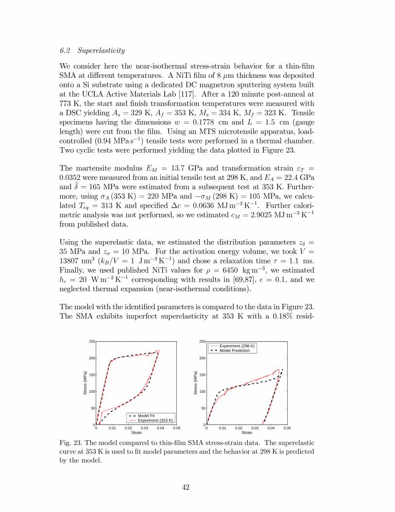
6.2 Superelasticity

We consider here the near-isothermal stress-strain behavior for a thin-filmSMA at different temperatures. A NiTi film of 8 µm thickness was depositedonto a Si substrate using a dedicated DC magnetron sputtering system builtat the UCLA Active Materials Lab [117]. After a 120 minute post-anneal at773 K, the start and finish transformation temperatures were measured witha DSC yielding As = 329 K, Af = 353 K, Ms = 334 K, Mf = 323 K. Tensilespecimens having the dimensions w = 0.1778 cm and L = 1.5 cm (gaugelength) were cut from the film. Using an MTS microtensile apparatus, load-controlled (0.94 MPa s−1) tensile tests were performed in a thermal chamber.Two cyclic tests were performed yielding the data plotted in Figure 23.

The martensite modulus EM = 13.7 GPa and transformation strain εT =0.0352 were measured from an initial tensile test at 298 K, and EA = 22.4 GPaand δ = 165 MPa were estimated from a subsequent test at 353 K. Further-more, using σA (353 K) = 220 MPa and −σM (298 K) = 105 MPa, we calcu-lated Teq = 313 K and specified ∆c = 0.0636 MJm−3K−1. Further calori-metric analysis was not performed, so we estimated cM = 2.9025 MJm−3K−1

from published data.

Using the superelastic data, we estimated the distribution parameters zδ =35 MPa and zσ = 10 MPa. For the activation energy volume, we took V =13807 nm3 (kB/V = 1 Jm−3K−1) and chose a relaxation time τ = 1.1 ms.Finally, we used published NiTi values for ρ = 6450 kgm−3, we estimatedhc = 20 Wm−2K−1 corresponding with results in [69,87], = 0.1, and weneglected thermal expansion (near-isothermal conditions).

The model with the identified parameters is compared to the data in Figure 23.The SMA exhibits imperfect superelasticity at 353 K with a 0.18% resid-

0 0.01 0.02 0.03 0.04 0.050

50

100

150

200

250

Strain

Str

ess

(MP

a)

0 0.01 0.02 0.03 0.04 0.050

50

100

150

200

250

Strain

Str

ess

(MP

a)

Experiment (298 K)Model Prediction

Model FitExperiment (353 K)

Fig. 23. The model compared to thin-film SMA stress-strain data. The superelasticcurve at 353 K is used to fit model parameters and the behavior at 298 K is predictedby the model.

42

ual strain. The model accurately predicts the asymmetric loading-unloadingcurves and the residual strain. At 298 K, the observed transformation is fromself-accommodating martensite to detwinned martensite. Using the fit to thesuperelastic data, we predicted the response at 298 K. We note that bothdata correspond to partial cycles, as full transformations are not observed.

6.3 Shape Memory Effect

The final example we consider is the shape memory effect exhibited by a thin-film SMA. Details of the fabrication and preparation of the test samples areprovided in [51]. A near-equiatomic NiTi film of 9 µm thickness was depositedonto a glass substrate using an RF magnetron sputtering system and was postannealed at 773 K. Samples with dimensions of w = 1mm and L = 5mmweretested in a temperature-controlled microtensile tester. The SMA was loadedat high temperature (austenite) after which cooling and re-heating took placeat 10 K/min under a fixed load. A total of 18 cyclic tests were preformed atfixed stresses ranging from 20 MPa to 600 MPa. Data from four of the testswere provided and are shown in Figure 24.

Since no calorimetric experiments were performed, we identified the modelparameters directly from the hysteresis data. We used the 200, 360, and 520MPa cases since it is likely the specimen did not fully transform at 40 MPa.We estimated the elastic moduli EA = 41.331 GPa and EM = 20.313 GPa,

200 300 400 500 6000

0.01

0.02

0.03

0.04

0.05

0.06

External Temperature (K)

Str

ain

200 300 400 500 6000

0.01

0.02

0.03

0.04

0.05

0.06

200 300 400 500 6000

0.02

0.04

0.06

0.08

Str

ain

200 300 400 500 6000

0.02

0.04

0.06

0.08

40MPa

360MPa(fit)

200MPa

520MPa

Fig. 24. The model (dashed) compared to thin-film SMA SME data (solid) at fixedstresses. The model is fit to the 360 MPa data and predicts the other cases.

43

and the transformation strain εT = 0.0388 from linear fits. Furthermore, wemeasured λA = 1.7 × 10−6 K−1 and λM = −21 × 10−6 K−1 from the 360MPa data. Identifying T σ

M for each curve and T σA for the 360 MPa case, we

calculated δ = 530 MPa, Teq = 344 K and ∆c = 0.9966 MJm−3K−1.

We estimated the distribution parameters zδ = 40 MPa and zσ = 80 MPa. Forthe activation energy volume, we took V = 13807 nm3 (kB/V = 1 Jm−3K−1)and chose a relaxation time τ = 0.8 ms. Finally, we used published NiTivalues ρ = 6450 kgm−3 and cM = 2.9025 MJm−3K−1 and we estimatedhc = 20 Wm−2K−1 and = 0.1.

The model is compared to the data in Figure 24. The SMA exhibits imper-fect shape memory at higher loads due to accumulating plastic strains, whichaccount for 32% of the transformation strain for the 520 MPa test. While themodel does predict a decrease in the effective transformation strain at lowerstresses, it underestimates the strain at 200 MPa and overestimates the strainat 40 MPa. Since we fit the model at 360 MPa where the accumulated strain is0.039, it is likely our initial fit did not properly characterize the transformationstrain of the material. Further thermal hysteresis tests should be consideredwhere plastic deformation is not as significant.

7 Concluding Remarks

We have presented a model quantifying the macroscopic nonlinear behavior ofshape memory alloys. In the first step of the development, we employed theframework of Müller-Achenbach-Seelecke to develop a local rate-dependent,thermomechanical model applicable to SMAs with uniform crystal lattices.Then we accommodated inhomogeneous and polycrystalline materials by av-eraging the variations of local material parameters and by considering nonuni-form stress fields. The result is a rate-dependent, fully thermomechanicalmodel that predicts relative elongation due to time-varying stress and tem-perature. We demonstrated that the model reasonably predicts the behaviorof SMA films pertinent to actuator design such as superelasticity and theshape memory effect.

The model admits a low-order formulation making it viable for incorporationinto engineering design applications and for implementation in model-basedcontrollers. In particular, control analysis has been employed for analogouspiezoceramic and magnetostrictive phase evolution models [80]. Moreover,the model provides a crucial step towards developing a unified methodologyfor modeling hysteresis in general ferroic materials [101].

The Boltzmann relations can yield a stiffODE system in (81) and full couplingbetween stress and temperature effects may require additional distributions.

44

Furthermore, statistical homogenization precludes the inverse problem of di-rectly constructing new material compounds based on performance require-ments.

There are opportunities for future research on the model. First, the devel-opment of control algorithms employing robust and multi-objective controlframeworks should be considered. Second, following further validation, themodel should be integrated into a finite element analysis infrastructure tosupport future design, performance evaluation, and qualification of thin-filmSMA microdevices.

Acknowledgments

The authors would like to thank the following for providing the SMA hysteresisdata used in this paper: Dr. Fuji Matsuzaki and Hisashi Naito at the Struc-tural Dynamics Lab within Nagoya University in Nagoya, Japan; Dr. Greg P.Carman, Jason Woolman, and Dr. K.P. Mohachandra from the Active Mate-rials Laboratory at UCLA in Los Angeles, CA; and Dr. Akira Ishida from theMaterials Engineering Laboratory at the National Institute for Materials Sci-ence in Tsukuba, Japan. This research was supported in part by the NationalScience Foundation under the grant CMS-0099764 and by the Air Force Officeof Scientific Research through the grant AFOSR-F49620-01-1-0107.

References

[1] R. Abeyratne and J.K. Knowles, “A continuum model of a thermoelasticsolid capable of undergoing phase transitions,” Journal of the Mechanics andPhysics of Solids, 41(3), pp. 541-571, 1993.

[2] R. Abeyaratne, K. Bhattacharya and J.K. Knowles, “Strain-energy functionswith multiple local minima: modeling phase transformations using finitethermoelasticity,” Nonlinear Elasticity: Theory and Applications, pp. 433-490(Ch. 12), Cambridge University Press, 2001.

[3] M. Achenbach, “A model for an alloy with shape memory,” InternationalJournal of Plasticity, Vol. 5, pp. 371-395, 1989.

[4] L.C. Andrews, Special Functions of Mathematics for Engineers, Second Ed.,Ch. 3.2, McGraw-Hill, Inc., New York, USA, 1992.

[5] F. Auricchio and E. Sacco, “Thermo-mechanical modelling of a superelasticshape-memory wire under cyclic stretching-bending loadings,” InternationalJournal of Solids and Structures, 38(35), pp. 6123-6145, 2001.

[6] G.R. Barsch, “Landau theory of structural transformations in titanium-nickeland gold-cadmium alloys,” Materials Science and Engineering: A, Vols. 273-275, pp. 161-165, 1999.

45

[7] G.R. Barsch, “Landau theory of the displacive phase transformations in gold-cadmium and titanium-nickel alloys,”Materials Science Forum, Vols. 327-328,pp. 367-376, 2000.

[8] P. Belík and M. Luskin, “A computational model for the indentation andphase transformation of a martensitic thin film,” Journal of the Mechanicsand Physics of Solids, 50(9), pp. 1789-1815, 2002.

[9] Y. Bellouard, T. Lehnert, et. al., “Local annealing of complex mechanicaldevices: a new approach for developing monolithic micro-devices,” MaterialsScience and Engineering: A, Vols. 273-275, pp. 795-798, 1999.

[10] Y. Bellouard, T. Lehnert, et. al., “Laser annealing of shape memory alloys:a versatile tool for developing smart micro-devices,” Journal de Physique IV(Proceedings), 11(8), pp. 571-576, 2001.

[11] W.L. Benard, H. Kahn, et. al., “Thin-film shape-memory alloy actuatedmicropumps,” Journal of Microelectromechanical Systems, 7(2), pp. 245-251,1998.

[12] K. Bhattacharya and R.V. Kohn, “Symmetry, texture and the recoverablestrain of shape-memory polycrystals,” Acta Materialia, 44(2), pp. 529-542,1996.

[13] K. Bhattacharyaa and R.D. James, “A theory of thin films of martensiticmaterials with applications to microactuators,” Journal of the Mechanics andPhysics of Solids, Vol. 47, pp. 531-576, 1999.

[14] A. Bhattacharyya, L. Sweeney and M.G. Faulkner, “Experimentalcharacterization of free convection during thermal phase transformations inshape memory alloy wires,” Smart Materials and Structures, 11(3), pp. 411-422, 2002.

[15] L.C. Brinson and M.S. Huang, “Simplifications and comparisons of shapememory alloy constitutive models,” Journal of Intelligent Material Systemsand Structures, Vol. 7, pp. 108-114, 1996.

[16] B. Bundara, M. Tokuda, et. al., “Superelastic tension and bendingcharacteristics of shape memory alloys,” Metals and Materials, 6(4), pp. 293-299, 2000.

[17] B. Bundara, “SMA: Present state and perspective for new applications,”Materials Science Forum, Vols. 327-328, pp. 43-46, 2000.

[18] S. Büttgenbach, S. Bütefisch, et. al., “Shape memory microactuators,”Microsystem Technologies, 7(4), pp. 165-70, 2001.

[19] T. Castán, E. Vives and A. Planes, “Elastic constants of BCC binary alloysnear the A3B composition and their relation to martensitic transitions,”Journal of Physics: Condensed Matter, 2(7), pp. 1743-1752, 1990.

[20] C. Craciunescu and M. Wuttig, “Extraordinary damping of Ni—Ti double layerfilms,” Thin Solid Films, 379(1-2), pp. 173-175, 2000.

46

[21] R. DesRoches and M. Delemont, “Seismic retrofit of simply supported bridgesusing shape memory alloys,” Engineering Structures, 24(3), pp. 325-332, 2002.

[22] T. Duerig, A. Pelton and D. Stöckel, “An overview of nitinol medicalapplications,” Materials Science and Engineering: A, Vols. 273-275, pp. 149-160, 1999.

[23] F. Falk, “Landau theory of martensitic phase transitions,” Journal de PhysiqueColloque, 43(C-4 ), pp. 3-15, 1982.

[24] F. Falk, “Pseudoelastic stress-strain curves of polycrystalline shape memoryalloys calculated from single crystal data,” International Journal ofEngineering Science, 27(3), pp. 277-284, 1989.

[25] F. Falk, “Constitutive theories of shape memory alloys related tomicrostructure,” Proceedings of the SPIE, Vol. 2442, pp. 2-10, 1995.

[26] M.G. Faulkner, J.J. Amalraj and A. Bhattacharyya, “Experimentaldetermination of thermal and electrical properties of Ni—Ti shape memorywires,” Smart Materials and Structures, 9(5), pp. 632—639, 2000.

[27] J.E. Favelukis, A.S. Lavine and G.P. Carman, “An experimentally validatedthermal model of thin-film NiTi,” Smart structures and materials 1999: SmartStructures and Integrated Systems, Proceedings of the SPIE, Vol. 3668, Pt. 1-2,pp. 617-629, 1999.

[28] Y. Fu and H. Du, “Effects of film composition and annealing on residual stressevolution for shape memory TiNi film,” Materials Science and Engineering A,Vol. 342, pp. 236—244, 2003.

[29] Y. Fu, W. Huang, et. al. “Characterization of TiNi shape-memory alloy thinfilms for MEMS applications,” Surface and Coatings Technology, 145(1-3),pp. 107-112, 2001.

[30] H. Fujita and H. Toshiyoshi, “Micro actuators and their applications,” 29(9),pp. 637-640, 1998.

[31] B. Gabry, C. Lexcellent, et. al., “Thermodynamic modeling of the recoverystrains of sputter-deposited shape memory alloys Ti—Ni and Ti—Ni—Cu thinfilms,” Thin Solid Films, 372(1-2), pp. 118-133, 2000.

[32] V. Galhotra, V. Gupta, et. al., “Shape memory alloy based micro actuators,”ACTUATOR 2000: 7th International Conference on New Actuators, pp. 338-341, 2000.

[33] W.S. Galinaitis, D.S. Joseph and R.C. Rogers, “Parameter identificationfor Preisach models of hysteresis,” Proceedings of DETC’01: the ASMEDesign Engineering Technical Conference and Computers and Information inEngineering Conference, Vol. 6, Pt. B, pp. 1409-1417, 2001.

[34] K. Gall and H. Sehitoglu, “The role of texture in tension-compressionasymmetry in polycrystalline NiTi,” International Journal of Plasticity, 15(1),pp. 69-92, 1999.

47

[35] K. Gall, H. Sehitoglu and Y. Chumlakov, “NiTi experiments versus modeling:Where do we stand?” Smart Structures and Materials 2000: Active Materials:Behavior and Mechanics, Proceedings of the SPIE, Vol. 3992, pp. 536-547,2000.

[36] J.I. Gersten and F.W. Smith, The Physics and Chemistry of Materials, Ch. 4.6,John Wiley & Sons, New York, USA, 2001.

[37] J. Gill, D. Chang, et. al., “Manufacturing issues of thin film NiTimicrowrapper,” Sensors and Actuators A, Vol. 93, pp. 148—156, 2001.

[38] J. Gill, K. Ho and G.P. Carman, “Three-dimensional thin-film shape memoryalloy microactuator with two-way effect,” Journal of MicroelectromechanicalSystems, 11(1), pp. 68-77, 2002.

[39] D.S. Grummon, S. Nam and L. Chang, “Effect of superelastically deformingNiTi surface microalloys on fatigue crack nucleation in copper,” ShapeMemory Materials and Phenomena - Fundamental Aspects and ApplicationsSymposium, pp. 259-264, 1992.

[40] H.P. Ho, C.Y. Chung, et. al., “Novel far infrared imaging sensor based on theuse of titanium-nickel shape memory alloys,” Smart Structures, Devices, andSystems, Proceedings of the SPIE, Vol. 4935, pp. 69-73, 2002.

[41] L. Hou, “Processing, microstructure and thermomechanical behaviorof superelastic nickel-titanium thin films sputter-deposited at elevatedtemperatures,” Ph.D. Thesis, Dept. of Materials Science and Mechanics,Michigan State University, 1998.

[42] L. Hou and D.S. Grummon, “Transformational superelasticity in sputteredtitanium-nickel thin films,” Scripta Metallurgica, Vol. 33(6), pp. 989-995, 1995.

[43] L. Hou, T.J. Pence and D.S. Grummon, “Structure and thermal stability intitanium-nickel thin films sputtered at elevated-temperature on inorganic andpolymeric substrates,” Materials Research Society Symposium Proceedings,Vol. 360, pp. 369-374, 1995.

[44] W.M. Huang, J.P. Tan, et. al., “Design, testing, and simulation of NiTi shape-memory-alloy thin-film-based microgrippers,” Journal of Microlithography,Microfabrication, and Microsystems, 2(3), pp. 185-190, 2003.

[45] D. Hughes and J.T. Wen, “Preisach modeling of piezoceramic and shapememory alloy hysteresis,” Smart Materials and Structures, 6(3), pp. 287-300,1997.

[46] Y. Huo, “A mathematical model for the hysteresis in shape memory alloys,”Continuum Mechanics and Thermodynamics, 1(4), pp. 283-303, 1989.

[47] F.P. Incropera and D.P. DeWitt, Fundamentals of Heat and Mass Transfer,Fifth Ed., John Wiley and Sons, Inc., New York, USA, 2002.

[48] A. Ishida and V. Martynov, “Sputter-deposited shape-memory alloy thin films:properties and applications,” MRS-Bulletin, 27(2), pp. 111-114, 2002.

48

[49] A. Ishida, M. Sato, et. al., “Bimorph-type microactuator using TiNi shape-memory film,” Materials Science Forum, Vols. 394-395, pp. 487-490, 2002.

[50] A. Ishida, M. Sato, et. al., “Stress-strain curves of sputter-deposited Ti-Ni thinfilms,” Philisophical Magazine A, 80(4), pp. 967-980, 2000.

[51] A. Ishida, A. Takei, et. al., “Shape memory behavior of Ti-Ni thin filmsannealed at various temperatures,” Materials Research Society SymposiumProceedings, Vol. 360, pp. 381-385, 1995.

[52] A.P. Jardine, J. Bartley-Cho and J. Flanagan, “Improved design andperformance of the SMA torque tube for the DARPA Smart Wing Program.”Smart structures and materials 1999. Industrial and commercial applicationsof smart structures technologies., Vol. 3674, pp. 260-269, 1999.

[53] Y.M. Jin and G.J. Weng, “Micromechanics study of thermomechanicalcharacteristics of polycrystal shape-memory alloy films,” Thin Solid Films,376(1-2), pp. 198-207, 2000.

[54] A.D. Johnson, V. Martynov and V. Gupta, “Applications of shape memoryalloys: advantages, disadvantages, and limitations,” Micromachining andMicrofabrication Process Technology VII, Proceedings of the SPIE, Vol. 4557,pp. 341-351, 2001.

[55] S. Kakac and Y. Yener, Convective Heat Transfer, Second Ed., CRC Press,Boca Raton, USA, 1995.

[56] T. Kim, Q. Su and M. Wuttig, “Thermo-mechanical Ni50Ti50/Si compositethin film switch,”Materials Research Society Symposium Proceedings, Vol. 360,pp. 375-380, 1995.

[57] M. Kohl, D. Dittmann, et. al., “Shape memory microvalves based on thinfilms or rolled sheets,” Materials Science and Engineering A, Vols. 273—275,pp. 784—788, 1999.

[58] M. Kohl, D. Dittmann, et. al., “Thin film shape memory microvalves withadjustable operation temperature,” Sensors and Actuators A: Physical, 83(1-3), pp. 214-219, 2000.

[59] M. Kohl, B. Krevet and E. Just, “SMA microgripper system,” Sensors andActuators A: Physical, Vols. 97-98, pp. 646-652, 2002.

[60] M. Kohl and K.D. Skrobanek, “Linear microactuators based on the shapememory effect,” Sensors and Actuators A: Physical, 70(1-2), pp. 104-111, 1998.

[61] A.R. Krommer and C.W. Ueberhuber, Computational Integration, Ch. 5,SIAM, Philadelphia, USA, 1998.

[62] E. Kröner, “Statistical Modeling,” in Modelling Small Deformations ofPolycrystals, edited by J. Gittus and J. Zarka, pp. 229-291, 1986.

[63] P. Krulevitch, A.P. Lee, et. al., “Thin film shape memory alloymicroactuators,” Journal of Microelectromechanical Systems, 5(4), pp. 270-282, 1996.

49

[64] A. Ktena, D.I. Fotiadis, P.D. Spanos, et. al., “A Preisach model identificationprocedure and simulation of hysteresis in ferromagnets and shape-memoryalloys,” Physica B: Condensed Matter, 306(1-4), pp. 84-90, 2001.

[65] K. Kuribayashi, “Micro SMA actuator and motion control,” MHS2000.Proceedings of 2000 International Symposium on Micromechatronics andHuman Science, pp. 35-42, 2000.

[66] K. Kuribayashi and T. Fujii, “A new micro SMA thin film actuator prestrainedby polyimide,” MHA’98. Proceedings of the 1998 International Symposium onMicromechatronics and Human Science, pp. 165-170, 1998.

[67] D.C. Lagoudas and A. Bhattacharyya, “On the correspondence betweenmicromechanical models for isothermal pseudoelastic response of shapememory alloys and the Preisach model for hysteresis,” Mathematics &Mechanics of Solids, 2(4), pp. 405-440, 1997.

[68] D.C. Lagoudas and Z. Bo, “Thermomechanical modeling of polycrystallineSMAs under cyclic loading, Part II: material characterization and experimentalresults for a stable transformation cycle,” International Journal of EngineeringScience, 37(9), pp. 1141-1173, 1999.

[69] A.S. Lavine and G.P. Carman, “Thermomechanical Modeling of Thin FilmShape Memory Alloy Devices,” Thermal Science and Engineering, 8(4), pp. 13-25, 2000.

[70] A.P. Lee, D.R. Ciarlo, et. al., “A practical microgripper by fine alignment,eutectic bonding and SMA actuation,” Sensors and Actuators A: Physical,54(1-3), pp. 755-759, 1996.

[71] C. Lexcellent, S. Moyne, et. al., “Deformation behaviour associated withthe stress-induced martensitic transformation in Ti—Ni thin films and theirthermodynamical modelling,” Thin Solid Films, 324(1-2), pp. 184-189, 1998.

[72] E. Limpert, W.A. Stahel and M. Abbt, “Log-normal Distributions across theSciences: Keys and Clues,” Bioscience, 51(5), pp. 341-352, (2001).

[73] C.C. Ma, R. Wang, et. al., “Frequency response of TiNi shape memoryalloy thin film micro-actuators,” Proceedings of IEEE, the Thirteenth AnnualInternational Conference on Micro Electro Mechanical Systems, pp. 370-374,2000.

[74] E. Makino, T. Mitsuya and T. Shibata, “Dynamic actuation properties ofTiNi shape memory diaphragm,” Sensors and Actuators A: Physical, 79(2),pp. 128-135, 2000.

[75] V. Martynov, “TiNi thin films for microactuators and microdevices: Sputterdeposition and processing techniques,” Materials Science Forum, Vols. 426-432, pp. 3475-3480, 2003.

[76] J.E. Massad and R.C. Smith, "A Domain Wall Model for FerroelasticMaterials," Journal of Intelligent Material Systems and Structures, 7(7),pp. 455-471, 2003.

50

[77] Y. Matsuzaki, K. Funami and H. Naito, “Inner loops of pseudoelastic hysteresisof shape memory alloys: Preisach approach,” Smart Structures and Materials2002: Active Materials: Behavior and Mechanics, Proceedings of the SPIE,Vol. 4699, pp. 355-364, 2002.

[78] S. Miyazaki and A. Ishida, “Martensitic transformation and shape memorybehavior in sputter-deposited TiNi-based thin films,” Materials Science andEngineering A, Vols. 273—275, pp. 106—133, 1999.

[79] K. Mori, H. Li, et. al., “Patterned shape memory alloy films,” MaterialsTransactions, 43(5), pp. 951-955, 2002.

[80] J.M. Nealis and R.C. Smith, “Control techniques for high performancenonlinear smart systems," Smart Structures and Materials 2003, Proceedingsof the SPIE, Vol. 5049, pp. 221-232, 2003.

[81] W. Ni and D.S. Grummon, “Nanoindentation and wear behavior of nickel-titanium alloys and thin films,” Materials Research Society SymposiumProceedings, Vol. 697, pp.53-58, 2002.

[82] K. Otsuka and C.M.Wayman, Shape Memory Materials, Cambridge UniversityPress, Cambridge, United Kingdom, 1998.

[83] N. Papenfuß and S. Seelecke, “Simulation and control of SMA actuators,”Smart structures and materials 1999: Mathematics and control in smartstructures, Proceedings of the SPIE, Vol. 3667, pp. 586-595, 1999.

[84] E. Patoor and M. Berveiller, “Micromechanical modeling ofthe thermomechanical behavior of shape memory alloys,” Mechanics of Solidswith Phase Changes, pp. 121-188, 1997.

[85] J. Peirs, D. Reynaerts and H. Van-Brussel, “Scale effects and thermalconsiderations for micro-actuators,” Proceedings, 1998 IEEE InternationalConference on Robotics and Automation, Vol. 2, pp. 1516-1521, 1998.

[86] R. Philips, Crystals, Defects and Microstructures: Modeling Across Scales,Ch. 7.4.2, Cambridge University Press, Cambridge, UK, 2001.

[87] P.L. Potapov and E.P. Da Silva, “Time response of shape memory alloyactuators,” Journal of Intelligent Material Systems and Structures, 11(2),pp. 125-134, 2000.

[88] H. Prahlad and I. Chopra, “Comparative evaluation of shape memory alloyconstitutive models with experimental data,” Journal of Intelligent MaterialSystems and Structures, 12(6), pp. 383-394, 2001.

[89] H. Prahlad and I. Chopra, “Development of a strain-rate dependent model foruniaxial loading of SMA wires,” Journal of Intelligent Material Systems andStructures, 14(7), pp. 429-442, 2003.

[90] I. Roch, Ph. Bidaud, “Fabrication and characterization of an SU-8 gripperactuated by a shape memory alloy thin film,” Journal of Micromechanics andMicroengineering, 13(2), pp. 330-336, 2003.

51

[91] M. Rohde and A. Schüssler, “On the response-time behaviour of lasermicromachined NiTi shape memory actuators,” Sensors and Actuators A:Physical, 61(1-3), pp. 463-468, 1997.

[92] S. Saadat, M. Noori, et. al., “Using NiTi SMA tendons for vibration control ofcoastal structures,” Smart Materials and Structures, 10(4), pp. 695-704, 2001.

[93] B. Schroeder, C. Boller, et. al., “Comparative assessment of models fordescribing the constitutive behaviour of shape memory alloys,” Smartmaterials and structures: proceedings of the 4th European Conference onSmart Structures and Materials in conjunction with the 2nd InternationalConference on Micromechanics, Intelligent Materials, and Robotics, pp. 305-312, 1998.

[94] S. Seelecke and I. Müller, “Shape memory alloy actuators in smart structures- modeling and simulation,” ASME Applied Mechanics Reviews, to appear,2003.

[95] J.A. Shaw and S. Kyriakides, “Thermodynamic aspects of NiTi,” Journal ofthe Mechanics and Physics of Solids, 43(8), pp. 1243-1281, 1995.

[96] J.A. Shaw, “A thermomechanical model for a 1-D shape memory alloy wirewith propagating instabilities,” International Journal of Solids and Structures,39(5), pp. 1275-1305, 2002.

[97] D.D. Shin, G.P. Carman, “Operating frequency of thin film NiTi in fluidmedia,” Proceedings of 2001 ASME IMECE, MEMS Symposium, pp. 221-227,2001.

[98] D.D. Shin, K.P. Mohanchandra, et. al., “Miniature actuator using thin-filmshape-memory alloy,” Smart Structures and Materials 2003: Industrial andCommercial Applications of Smart Structures Technologies, Proceedings of theSPIE, Vol. 5054, pp. 118-124, 2003.

[99] Y. Shu, “Shape-memory micropumps,” Materials Transactions, 43(5), pp.1037-1044, 2002.

[100] J.F. Smith, Q. Jiang, et. al., “Cp and fractal phase transformation in the shapememory alloy Ni—52Ti ,” Materials Science and Engineering A, 149(1), pp.111-120, 1991.

[101] R.C. Smith, S. Seelecke, et. al., “A unified model for hysteresis in ferroicmaterials," Smart Structures and Materials 2003: Modeling, Signal Processing,and Control, Proceedings of the SPIE, Vol. 5049, pp. 88-99, 2003.

[102] T. Sterzl, B. Winzek, et. al., “Bistable shape memory thin film actuators,”Smart Structures and Materials 2003: Active Materials: Behavior andMechanics, Proceedings of the SPIE, Vol. 5053, pp. 101-109, 2003.

[103] V. Stoilov and A. Bhattacharyya, “A theoretical framework of one-dimensionalsharp phase fronts in shape memory alloys,” Acta Materialia, 50(20), pp. 4939-4952, 2002.

52

[104] M. Tabib-Azar, B. Sutapun and M. Huff, “Applications of TiNi thin filmshape memory alloys in micro-opto-electro-mechanical systems,” Sensors andActuators A: Physical, 77(1), pp. 34-38, 1999.

[105] H. Tamai and Y. Kitagawa, “Pseudoelastic behavior of shape memoryalloy wire and its application to seismic resistance member for building,”Computational Materials Science, 25(1-2), pp. 218-227, 2002.

[106] J. Uchil, K.P. Mohanchandra, et. al., “Study of critical dependence ofstable phases in Nitinol on heat treatment using electrical resistivity probe,”Materials Science and Engineering A, Vol. 251, pp. 58-63, 1998.

[107] J. Uchil, K.P. Mohanchandra, et. al., “Thermal expansion in various phases ofNitinol using TMA,” Physica B, Vol. 270, pp.289-297, 1999.

[108] A. Visitin, Differential Models of Hysteresis, Springer-Verlag, New York, 1994.

[109] R.X. Wang, Y. Zohar and M. Wong, “The effects of process-induced stress onthe microstructures and the phase transformation characteristics of sputteredtitanium—nickel thin-film shape-memory alloys,” Journal of Micromechanicsand Microengineering, 11(6), pp. 686-691, 2001.

[110] R.X. Wang, Y. Zohar and M. Wong, “Residual stress-loaded titanium—nickelshape-memory alloy thin-film micro-actuators,” Journal of Micromechanicsand Microengineering, 12(3), pp. 323-327, 2002.

[111] F. Warkusz, “The size effect and the temperature coefficient of total resistancein thin metal films,” Journal of Physics D-Applied Physics, Vol. 11, 1978.

[112] G. Webb, A. Kurdila and D. Lagoudas, “Adaptive hysteresis model for modelreference control with actuator hysteresis,” Journal of Guidance, Control, andDynamics, 23(3), pp. 459-465, 2000.

[113] K. Wilde, P. Gardoni and Y. Fujino, “Base isolation system with shapememory alloy device for elevated highway bridges,” Engineering Structures,23(3), pp. 222—229, 2000.

[114] B. Winzek, T. Sterzl, et. al., “Smart motion control by phase-coupledshape memory composites,” Proceedings of the 2002 IEEE/RSJ InternationalConference on Intelligent Robots and Systems, Vols. 1-3, pp. 2004-2009, 2002.

[115] B. Winzek, S. Schmitz, et. al., “SMA-thin film composites providing travelingwaves,” Smart structures and materials 2003: Active Materials: Behavior andMechanics, Proceedings of the SPIE, Vol. 5053, pp. 110-118, 2003.

[116] D. Wood, J.S. Burdess and A.J. Harris, “Actuators and their mechanismsin microengineering,” Engineering Science and Education Journal, 7(1), pp.19-27, 1998.

[117] J.L. Woolman, K.P. Mohanchandra and G.P. Carman, “Composition andannealing effects on the mechanical properties of superelastic thin film nickeltitanium,” Smart Structures and Materials 2003, Proceedings of the SPIE,Vol. 5053, pp. 230-238, 2003.

53

[118] M.R. Wuttig, “Thin film SMA/Si composite actuators ,” Smart Structures andMaterials 2000: Mathematics and Control in Smart Structures, Proceedings ofthe SPIE, Vol. 3984, pp. 450-455, 2000.

[119] D. Xu, L. Wang, et. al., “Characteristics and fabrication of NiTi/Si diaphragmmicropump,” Sensors and Actuators A: Physical, 93(1), pp. 87-92, 2001.

[120] Y.Y. Ye, C.T. Chan and K.M. Ho, “Structural and electronic properties ofthe martensitic alloys TiNi, TiPd, and TiPt,” Physical Review B, 56(7), pp.3678—3689, 1997.

[121] H. Zhang, Y. Bellouard, et. al., “A monolithic shape memory alloymicrogripper for 3-D assembly of tissue engineering scaffolds,” Microroboticsand Microassembly III, Proceedings of the SPIE, Vol. 4568, pp. 50-60, 2001.

54