A History of Modern Weather Forecasting

The Stone Age

• Prior to approximately 1955, forecasting was basically a subjective art, and not very skillful.

• Observations were sparse, with only a few scattered ship reports over the oceans.

• The technology of forecasting was basically subjective extrapolation of weather systems, in the latter years using the upper level flow (the jet stream).

• Local weather details—which really weren’t understood-- were added subjectively.

UpperLevelChart

The Development of NWP• Vilhelm Bjerknes in his landmark

paper of 1904 suggested that NWP was possible.– A closed set of equations existed

that could predict the future atmosphere (primitive equations)

– But it wasn’t practical then because there was no reasonable way to do the computations and sufficient data for initialization did not exist.

Numerical Weather Prediction• The advent of digital computers in the late

1940s and early 1950’s made possible the simulation of atmospheric evolution numerically.

• The basic idea is if you understand the current state of the atmosphere, you can predict the future using the basic physical equations that describe the atmosphere.

Numerical Weather PredictionOne such equation is Newton’s Second Law:

F = maForce = mass x acceleration

Mass is the amount of matter

Acceleration is how velocity changes with time

Force is a push or pull on some object (e.g., gravitational force, pressure forces, friction)

This equation is a time machine!

Using a wide range of weather observations we can create a three-dimensional description of the atmosphere… known as the initialization

Numerical Weather Prediction

•This gives the distribution of mass and allows us to calculate the various forces.

•Then… we can solve for the acceleration using F=ma

•But this gives us the future…. With the acceleration we can calculate the velocities in the future.

•Similar idea with temperature and humidity.

Numerical Weather Prediction

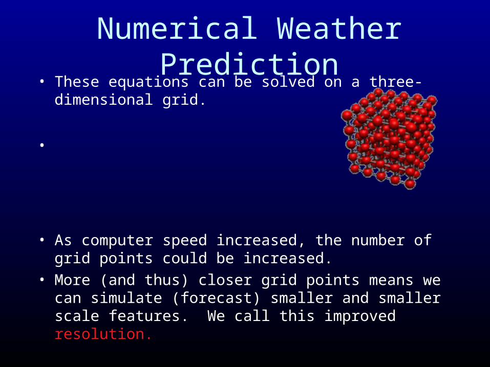
Numerical Weather Prediction• These equations can be solved on a three-dimensional grid.

•

• As computer speed increased, the number of grid points could be increased.

• More (and thus) closer grid points means we can simulate (forecast) smaller and smaller scale features. We call this improved resolution.

NWP Becomes Possible

• By the 1940’s there was an extensive upper air network, plus many more surface observations. Thus, a reasonable 3-D description of the atmosphere was possible.

• By the mid to late 1940’s, digital programmable computers were becoming available…the first..the ENIAC

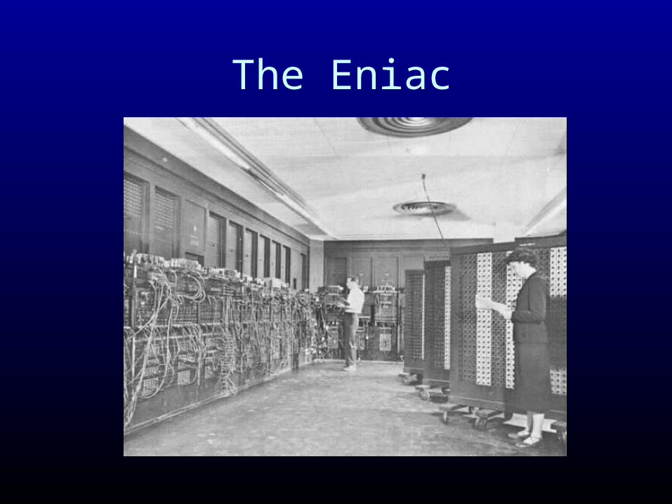
The Eniac

First NWP• The first successful numerical prediction of

weather was made in April 1950, using the ENIAC computer at Maryland's Aberdeen Proving Ground

• The prediction was for 500 mb height, covered North America, used a two-dimensional grid with 270 points about 700 km apart.

• The results indicated that even primitive NWP was superior to human subjective prediction. The NWP era had begun.

Evolving NWP

• Early 50s: one-level baratropic model• Late 50s: Two-level baroclinic QG model (just

like Holton!)• 1960s: Primitive Equation Models of increasing

resolution and number of levels.• Resolution increases (distance between grid points

decrease): 1958: 380 km, 1985: 80 km, 1995: 40 km, 2000: 22 km, 2002: 12 km

A Steady Improvement

• Faster computers and better understanding of the atmosphere, allowed a better representation of important physical processes in the models

• More and more data became available for initialization

• As a result there has been a steady increase in forecast skill from 1960 to now.

Forecast Skill Improvement

ForecastError

Year

Better

National Weather Service

Forecaster at the Seattle National Weather Service Office

The National Weather Service