A Guide to Elections Forensics Research and Innovation Grants Working Papers Series July 28, 2017

Publication Date

A Guide to Election Forensics Research and Innovation Grants Working Papers Series Allen Hicken University of Michigan Walter R. Mebane, Jr. University of Michigan July 28, 2017

TABLE OF CONTENTS

EXECUTIVE SUMMARY ................................................................................................................... 1

BACKGROUND ............................................................................................................................. 3

THE ROLE FOR ELECTION FORENSICS .................................................................................................. 6 A. A Primer on Election Forensics Methods ................................................................................... 7 B. Key Statistical Methods ........................................................................................................... 8 C. Examples of Election Forensics Analysis ................................................................................. 12

STATUS OF ELECTION FORENSICS METHODS ...................................................................................... 30

REFERENCES .............................................................................................................................. 32

APPENDIX A: DIGIT AND DISTRIBUTION APPROACHES ......................................................................... 37

MESSAGE FROM THE DRG CENTER ACTING DIRECTOR USAID’s Center of Excellence in Democracy, Human Rights, and Governance (DRG Center) is pleased to share A Guide to Election Forensics. This publication, together with the Election Forensics Toolkit DRG Center Working Paper and the online Election Forensics Toolkit, were produced by USAID in partnership with the University of Michigan and the Institute of International Education as part of the Research and Innovation Grants Working Papers Series. The Strategy on Democracy, Human Rights, and Governance1 reaffirmed USAID’s commitment to “generate, analyze, and disseminate rigorous, systematic, and publicly accessible evidence in all aspects of DRG policy, strategy and program development, implementation, and evaluation.” This paper, along with the others in the series, makes a valuable contribution to advancing this commitment to learning and evidence-based programming. This series is part of USAID’s Learning Agenda for the DRG Sector, a dynamic collection of research questions that serves to guide the DRG Center’s and USAID field missions’ analytical efforts. USAID seeks to inform strategic planning and project design efforts with the very best theory, evidence, and practical guidance. Through these efforts, the Learning Agenda is contributing to USAID’s objective to support the establishment and consolidation of inclusive and accountable democracies to advance freedom, dignity, and development. The research presented in this Guide to Election Forensics, in the more detailed DRG Center Working Paper, and in the online tool explains the role election forensics can play in verifying the integrity of election data, demonstrates several statistical tests used in election forensics to verify election data, and illustrates how those tests identify anomalous patterns in the data that can indicate intentional manipulation of results. The Guide also provides a more general introduction to election forensics as a field; the DRG Center Working Paper focuses on presenting in detail the results of applying election forensics to specific recent elections in Afghanistan, Albania, Bangladesh, Cambodia, Kenya, Libya, South Africa, and Uganda; and the online Election Forensics Toolkit allows practitioners to access the results of forensic analysis on the data from many elections and to upload electoral data for future analysis. I hope you find this research enlightening and helpful. As the DRG Center’s Learning Agenda progresses, we will continue our effort to bring forward the latest in relevant social science research to important constituencies for our work, particularly our DRG cadre and implementing partners, but also others. I invite you to stay involved as this enriching, timely, and important work proceeds. Madeline Williams, Acting Director Center of Excellence on Democracy, Human Rights, and Governance US Agency for International Development

1 https://www.usaid.gov/sites/default/files/documents/1866/USAID%20DRG_%20final%20final%206-24%203%20(1).pdf

ACRONYM LIST 2BL Second-Digit Benford’s Law-like ANC African National Congress BNP Bangladesh National Party C05s Count Last-Digit 0/5 Indicator Mean Dem Al Democratic Alliance DipT Unimodality Test p-Value EFF Economic Freedom Fighters

EM Expectation-Maximization Kurt Kurtosis LastC Last-Digit Mean OECD Organisation for Economic Cooperation and Development P05s Percentage Last-Digit 0/5 Indicator Mean Skew Skewness

University of Michigan USAID/DCHA/DRG Working Papers Series 1

EXECUTIVE SUMMARY There is an acute need for methods of detecting and investigating fraud in elections, because the consequences of electoral fraud are grave for democratic stability and quality. When the electoral process is compromised by fraud, intimidation, or even violence, elections can become corrosive and destabilizing—sapping support for democratic institutions; inflaming suspicion; and stimulating demand for extra-constitutional means of pursuing political agendas, including violence. Accurate information about irregularities can help separate false accusations from evidence of electoral malfeasance. Accurate information about the scope of irregularities can also provide a better gauge of election quality. Finally, accurate information about the geographic location of malfeasance—the locations where irregularities occurred and how they cluster—can allow election monitors and pro-democracy organizations to focus attention and resources more efficiently and to substantiate their assessments of electoral quality. Through a Research and Innovation Grant funded by USAID’s Center of Excellence on Democracy, Human Rights, and Governance under the Democracy Fellows and Grants Program, a research team from the University of Michigan, led by Professors Walter Mebane and Allen Hicken, built an innovative online tool, the Election Forensics Toolkit, that allows researchers and practitioners to conduct complex statistical analysis on detailed, localized data produced through the electoral process. The Election Forensics Toolkit presents results in a variety of ways—including detailed country maps showing “hot spots” of potential fraud—that allow practitioners not only to see where electoral fraud may have occurred but also the probability that the disturbances in the election data that the statistical analyses detect are attributable to fraud, rather than to other cultural or political influences, such as gerrymandering or geographic distribution of voting constituencies, among others. Election forensics is an emerging field in which scholars use a diverse set of statistical tools—including techniques similar to those developed to detect financial fraud—to analyze numerical electoral data and detect where patterns deviate from those that should occur naturally, following demonstrated mathematical principles. Numbers that humans have manipulated present patterns that are unlikely to occur if produced by a natural process—such as free and fair elections or normal commercial transactions. These deviations suggest either that the numbers were intentionally altered or that other factors—such as a range of normal strategic voting practices—influenced the electoral results. The greater the number of statistical tests that identify patterns that deviate from what is expected to naturally occur, the more likely that the deviation results from fraud rather than legal strategic voting. Compared to existing methods of electoral transparency such as in-person monitoring and parallel vote tabulations, election forensics has three key advantages:

1. It relies on objective data, such as reported election results disaggregated to the level of electoral constituencies, precincts, and/or polling stations.

2. It allows for systematic analysis of reported votes from all contests in all localities. 3. It products estimates of fraud that include statistical statements about the confidence of

conclusions.

University of Michigan USAID/DCHA/DRG Working Papers Series 2

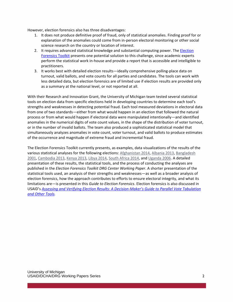
However, election forensics also has three disadvantages: 1. It does not produce definitive proof of fraud, only of statistical anomalies. Finding proof for or

explanation of the anomalies could come from in-person electoral monitoring or other social science research on the country or location of interest.

2. It requires advanced statistical knowledge and substantial computing power. The Election Forensics Toolkit presents one potential solution to this challenge, since academic experts perform the statistical work in-house and provide a report that is accessible and intelligible to practitioners.

3. It works best with detailed election results—ideally comprehensive polling-place data on turnout, valid ballots, and vote counts for all parties and candidates. The tools can work with less detailed data, but election forensics are of limited use if election results are provided only as a summary at the national level, or not reported at all.

With their Research and Innovation Grant, the University of Michigan team tested several statistical tools on election data from specific elections held in developing countries to determine each tool’s strengths and weaknesses in detecting potential fraud. Each tool measured deviations in electoral data from one of two standards—either from what would happen in an election that followed the natural process or from what would happen if electoral data were manipulated intentionally—and identified anomalies in the numerical digits of vote count values, in the shape of the distribution of voter turnout, or in the number of invalid ballots. The team also produced a sophisticated statistical model that simultaneously analyzes anomalies in vote count, voter turnout, and valid ballots to produce estimates of the occurrence and magnitude of extreme fraud and incremental fraud. The Election Forensics Toolkit currently presents, as examples, data visualizations of the results of the various statistical analyses for the following elections: Afghanistan 2014, Albania 2013, Bangladesh 2001, Cambodia 2013, Kenya 2013, Libya 2014, South Africa 2014, and Uganda 2006. A detailed presentation of these results, the statistical tools, and the process of conducting the analyses are published in the Election Forensics Toolkit DRG Center Working Paper. A shorter presentation of the statistical tools used, an analysis of their strengths and weaknesses—as well as a broader analysis of election forensics, how the approach contributes to efforts to ensure electoral integrity, and what its limitations are—is presented in this Guide to Election Forensics. Election forensics is also discussed in USAID’s Assessing and Verifying Election Results: A Decision-Maker’s Guide to Parallel Vote Tabulation and Other Tools.

University of Michigan USAID/DCHA/DRG Working Papers Series 3

BACKGROUND Election forensics are an emergent means by which to isolate potential anomalies in and diagnose the accuracy of reported election results, using statistical techniques that can identify patterns and assess their chances of occurring by chance. The purpose of this Guide is to help orient users about how best to use election forensics as one constructive tool among several in election assistance and monitoring efforts, serving as a complement to an Election Forensics Toolkit that implements several of the methods. The Guide discusses the strengths and weaknesses of election forensics relative to other tools for evaluating the integrity of elections, as well as the different types of forensic methods and their respective advantages and limitations. The Guide describes foundations of these methods and the calculations they involve, and it offers guidance on interpreting results, including in a comparative context. The use of the methods is demonstrated through illustrative case studies. Under the best conditions, elections allow citizens to express their preferences; provide information about favored issues, stances, and policies; connect voters to their governments; hold representatives and other leaders accountable; and settle social divisions that could otherwise become violent. When elections are widely viewed as free and fair, this outcome reduces the likelihood that winners and losers in the election contests will take actions that undermine democratic foundations with destabilizing effects. If the contestants believe that they can participate in a regular election contest with transparency and fairness, and they endorse the electoral rules, then legitimacy, trust, and stability in society is enhanced and progressively entrenched (Dahl 1971). While elections are not sufficient by themselves to constitute a full, mature democracy (Zakaria 1997), comparative empirical evidence shows that conducting elections—especially if they are accepted and allow true competition accompanied by the prospect of alternation in power—can contribute to a virtuous cycle even under difficult conditions (Lindberg 2006). Departures from this ideal, however, are not uncommon, especially in new and fragile democracies. Election malfeasance can take a variety of forms, including the intimidation of voters, violence against candidates and their supporters, and outright election fraud. Regardless of the type of malfeasance, when the electoral process is perceived to be significantly flawed or biased, and the final results suspect or rigged, then the salutary effects of elections can evaporate. Instead of building trust and stability, elections can become corrosive and destabilizing—sapping support for democratic institutions, inflaming suspicion, and stimulating demand for extra-constitutional means of pursuing political agendas. In short, electoral malfeasance can distort and destabilize democracy. Malfeasance can affect electoral outcomes (including which contestants win public office), influence whether or not the results are accepted as legitimate, and shape the extent to which elections produce subsequent political and social stability. An aim of this guide is to summarize and reflect on ways of mitigating these complications. The focus includes electoral malfeasance surrounding the counting of votes. Such malfeasance ranges from glitches and indications of minor malfeasance in the processes (all too prevalent even in Organisation for Economic Cooperation and Development countries), to more serious instances involving actual or apparent manipulation of results, including fraudulent or fictitious figures reported by the government. Instances of malfeasance have been relatively common around the world. During the first half of 2015

University of Michigan USAID/DCHA/DRG Working Papers Series 4

alone, for example, allegations of election fraud occurred in Bangladesh, India, Israel, Macedonia, Nigeria, Pakistan, Russia, Togo, the United Kingdom, the United States, and Zambia. These allegations run the gamut from minor irregularities in isolated polling locations to systematic fraud at a national scale. More comprehensively, data compiled by Kelley and Kolev (2010) on national elections conducted in more than 170 countries from 1978-2004 indicate the following:

▪ 61% of countries experienced some degree of (known) cheating, including fraud related to the tabulation of votes, with 27% of countries exhibiting major problems;

▪ 25% of the legislative elections and 15% of the presidential elections were plagued by cheating; and

▪ These issues are persistent, affecting more than half of the elections conducted in 2000 and nearly half in 2002-2004.

An immediate consequence of such malfeasance can be controversy about the results raised by parties and candidates (and their supporters), especially those in the opposition. Data compiled by Lindberg (2006) on national elections held in Africa from 1989-2007 highlights the importance of the perceived integrity of the election process and results:

▪ Of elections rated as free and fair, 93% were accepted by all of the main losing parties; ▪ Of elections with minor irregularities, 49% were accepted by all of the main losing parties, 39%

exhibited partial acceptance (either by some of the main losing parties, but not all, or not by all of them at first, but eventually), and 12% were not accepted;

▪ Of elections with substantial irregularities that affected the results, 2% were accepted by all of the main losing parties, 40% exhibited partial acceptance, and 58% were not accepted; and

▪ Of elections that were rated as not free and fair, none were accepted by all of the main losing parties, 9% exhibited partial acceptance, and 91% were not accepted.

These controversies are hardly limited to public debate and dissent. Instead, they can quickly turn violent. A conspicuous recent example is the large-scale turmoil after Kenya’s disputed 2007 presidential election, leading to more than 1,000 deaths. Other similar cases have been observed elsewhere in Africa (e.g., Côte d’Ivoire, Nigeria, Zimbabwe) and around the world. Given the ubiquity of fraud allegations, what methods are available to observers to assess the credibility of such claims? Can the same methods be used to confirm the fairness of an election in the absence of fraud allegations? There is an acute need for methods of detecting and investigating fraud. First, accurate information on electoral irregularities can help separate false accusations from true evidence of electoral malfeasance. Second, accurate information about the scope of irregularities can provide election monitors with a better gauge of the quality of elections. Third, accurate information about the geography of malfeasance—the locations where irregularities are observed and how they cluster—can bolster the activities of election monitors and pro-democracy organizations, among other things allowing them to focus their attention and resources more efficiently and helping them to substantiate their assessments of the quality of elections. Ideally, a method for detecting electoral fraud should meet each of the following criteria:

▪ The method should be sensitive enough to detect anomalies. We want to avoid mislabeling problematic elections as problem-free. In other words, we want to limit false negatives.

University of Michigan USAID/DCHA/DRG Working Papers Series 5

▪ The method should accurately detect anomalies. The method should reveal anomalies when they arise, but produce null results when no anomalies are present. In other words, we want to limit false positives.

▪ The method should involve systematic observation. In order avoid potential bias, wherever possible we want to analyze electoral results in their entirety, ideally at the most fine-grained level possible. This approach is preferable to limited descriptive evidence and select case studies.

▪ The method should enable the identification of where, geographically, anomalies have occurred. While it is helpful to know that anomalies exist, ideally methods will identify the locations where those anomalies occur. This facilitates additional analysis and validation and enables more effective responses. Geographic analysis can also take into account the possibility that anomalies may cluster together and be related to other relevant political, cultural, or ethnic factors.

▪ The method should produce estimates of uncertainty, indicating how confident we can be in our conclusions. A method need not yield definitive findings to be worthwhile in this setting. Absent definitive findings, a measure of the extent to which the results are likely to be valid is crucial.

Scholars, aid agencies, and policymakers are devoting increasing attention to detecting election irregularities and trying to improve election processes. Current efforts to promote the integrity of elections around the world are multi-pronged. They include designing electoral systems and procedures in accordance with standards of best practice, promoting the development and capacity of independent election agencies, ballot reform, and on-the-ground monitoring of elections by domestic and foreign observers. The last of these—on-the-ground monitoring—addresses a direct form of malfeasance: manipulating the results, when they are counted, tabulated, or reported. In an effort to combat this problem, political parties often undertake their own monitoring, setting up a presence at polling stations and observing or even involving themselves directly in the process of recording votes (e.g., parallel vote tabulations). Another especially effective approach has been reporting of results of exit polls in near-real time, using mobile phone-based tools, as was observed originally in the Ukraine in 2004. More generally, election monitoring by independent observers from civil society, the media, and international organizations has become commonplace (Hyde 2011, Kelley 2012). Social scientists have been adding to these efforts. For example they have evaluated methods to reduce the manipulation of results, e.g., using communications technology to take photos of tabulations at polling stations (Callen, Long, and Isaqzadeh 2011; Callen and Long 2013; Callen, Gibson, Jung, and Long 2013). Election monitoring and observation is often conducted in person. Yet, in-person observation has certain inherent limitations. The monitors themselves, especially individuals from within a given country, may not be impartial. Those on the losing side have incentives to claim that results are fraudulent, whether or not this is true, in an effort to gain leverage or disrupt the process. Likewise those on the winning side have incentives to conclude that the elections were free and fair. Even if observers are independent, their access to polling places may be restricted by the government or by local authorities. In addition, observers may not be able to blanket an entire country for logistical, financial, political, or safety reasons. Even where full access and coverage are feasible, the detailed information collected by observers is rarely made available publicly, especially in a comprehensive fashion at the level of electoral constituencies, let alone precincts and polling stations. Instead, the information is generally compiled

University of Michigan USAID/DCHA/DRG Working Papers Series 6

into summary reports, which may feature select anecdotal examples of malfeasance. These reports usually offer an overall judgment about whether an election was free and fair, which is not necessarily immune to politicization because of the stakes that may be involved. In-person observation can be a valuable input into assessments of electoral fraud, but rarely offers a comprehensive evaluation of individual contests such as those for specific parliamentary seats. Meanwhile, the prospect of scholars setting up on-the-ground experimental interventions to address fraud in elections around the world is unrealistic, since this would again require the necessary access, as well as massive personnel, financial, and technological resources.

THE ROLE FOR ELECTION FORENSICS As useful as any existing method may be, none meets all of the ideal criteria outlined in the previous section. In this regard, new and developing methods in election forensics offer tools that can conceivably meet all of our ideal criteria. Scholars in the field of election forensics have been developing techniques designed to detect the presence of fraud or malfeasance in an election, and estimate its magnitude, based on characteristics of the reported results. Some of the election forensic methods adopt techniques similar to those developed by people seeking to detect financial fraud. One basic idea the methods share is that numbers manipulated by humans typically have patterns of digits that are unlikely to have arisen through a “natural” process—such as a free and fair election or normal commercial transactions. In essence, numeric manipulations (frauds) tend to leave distinctive traces. If election results have unnatural patterns, those anomalies should be detectable using statistical techniques. Relative to existing approaches, election forensics methods have at least three key advantages. First, election forensics relies on reported election results, disaggregated to the level of electoral constituencies, precincts, and/or polling stations. These results are “objective” in the sense that they are used exactly as reported—forensic methods analyze the official record, which are the public basis of election outcomes. By contrast, the observations and judgments of individual election monitors, country experts, or assessment teams can be (or be accused of being) selective and subjective. Second, election forensics allows for the systematic analysis of all reported votes from all contests in all localities—even those locations where observers do not have access for political, security, or logistical reasons. Third, election forensics produces estimates of fraud that include information about the confidence of conclusions, as opposed to observations methods that lack these metrics beyond some vague expression of certainty versus uncertainty, which may not be well founded. At the same time, election forensics have three primary disadvantages. First, producing the statistics does require a fairly sophisticated knowledge of quantitative methods, as well as substantial computing power. The Electoral Forensics Toolkit presents one potential solution to overcome this challenge: experts perform the statistical work in-house and provide a report of the results that is accessible and intelligible to non-specialists. Second, election forensics do not produce definitive proof of fraud—unlike direct observation of ballot box stuffing. Instead, the method produces probabilistic evidence of anomalies that are suggestive of fraud. This limitation need not fundamentally undermine the election forensics approach, especially given that other methods of election assessment are similarly constrained (again, short of tangible proof of malfeasance). Rather, the limitations of election forensics should

University of Michigan USAID/DCHA/DRG Working Papers Series 7

caution against making overstated inferences or claiming that the approach can supplant all others, errors that we are conscious to emphasize as concerns and to avoid. Third, the utility of election forensics methodology is limited if election results are not reported in a sufficiently detailed fashion. The method works best the more detailed and disaggregated the data are. The ideal is comprehensive data on turnout, and valid and spoilt ballots, together with all votes for all parties and candidates down to each and every polling place (or even down to every ballot box), though the tools can also work with less detailed data. Election forensics are of limited use, however, if election results are provided only as a summary at a national level, or not reported at all (e.g., some countries only report who was elected, or the distribution of seats among the parties contesting the election). In these cases, assessment tools other than election forensics are more appropriate—and may be the only realistic options. Fortunately, a vast majority of countries do provide subnational election results. In fact, even many countries that conduct elections in a context marked by severe restrictions on political mobilization and competition, with boycotts and/or accusations of fraud by opposition parties, still report subnational results. The availability of these detailed results allows election forensics to be married with complementary methods and tools, such as in-person monitoring. Election forensics enhance the value of more labor-intensive forms of monitoring, instead of being a wholesale substitute. Anomalies and other actual or suggestive evidence of malfeasance detected by one or more approaches can be combined in ways that are mutually reinforcing. For example, users might combine our estimates of anomalies with information from country officers or election observers, which may be reflected in datasets such as the Electoral Integrity Project, Kelly and Kolev’s Quality of Elections Database, or Lindberg’s Elections and Democracy in Africa to produce a more complete, cross-validated picture of a given election.2

A. A Primer on Election Forensics Methods Two assumptions underlie the use of election forensics. First, statistical analysis of suitably disaggregated election data can detect instances of illegitimate human manipulation. Second, patterns in data that typically result from such manipulation, as well as patterns of deviations from the distributions that are expected in the absence of manipulation, are more likely to represent evidence of fraud, if found consistently across multiple statistical techniques. A variety of methods has been used to evaluate election results as indicators of anomalies. Past research has focused on several kinds of data reported by government election authorities: voter turnout, votes received by various parties or candidates, and number of ballots deemed invalid. Some researchers analyze combinations of these reported data. The research can go in one of two directions. One assumes what should happen in an election where anomalies do not occur. The other takes the complementary approach and assumes what should happen if manipulations are attempted. Different statistical methods may respond to different kinds of anomalies. When the various methods lead to similar statistical indications—e.g., indications that there is a high likelihood that there are anomalies in reported data—it adds strength to our conclusions (i.e., that election results have been manipulated).

2 Electoral Integrity Project: http://www.electoralintegrityproject.com/. Quality of Elections Database: http://sites.duke.edu/kelley/data/. Elections and Democracy in Africa: http://www.clas.ufl.edu/users/sil/downloads.html.

University of Michigan USAID/DCHA/DRG Working Papers Series 8

The first approach to anomaly and fraud detection centers on the digits of the vote count values as indicators of anomalies. The first digits of aggregate vote totals (Cantu and Saiegh 2011), second significant digits (Pericchi and Torres 2011), and the last digits (Beber and Scacco 2012) have all been of interest. The second digit methods are based on the idea that non-anomalous vote counts follow the so-called second-digit Benford’s Law-like (2BL) distribution—a particular distribution of numerical digits occurring from a natural process with each number 0-9 as differentially likely (Pericchi and Torres 2004; Mebane 2006). The last-digit method is based on the idea that unmanipulated vote counts have uniformly distributed 0-9 last digits. The digit-focused methods are controversial as fraud-detection devices (Carter Center 2005; Shikano and Mack 2009; L´opez 2009; Deckert, Myagkov, and Ordeshook 2011; Mebane 2011, 2014), with in particular Mebane (2013a, n.d.) claiming that the second digits of precinct vote counts may be produced by normal political processes such as strategic voting and mobilization that do not trace back to illegitimate human manipulation. A second approach relies on analysis of turnout data. This approach focuses on departures from the expected shape of the distribution of voter turnout (Myagkov, Ordeshook, and Shaikin 2009; Levin, Cohn, Ordeshook, and Alvarez 2009) or on the relationship between turnout and the share of votes for the leading candidate (Buzin and Lubarev 2008). Also particular patterns in turnout and vote proportions have been identified because they facilitate coordination among election malefactors (Kalinin and Mebane 2011, Mebane 2013b). Third, invalid vote counts have also been useful in diagnosing possible irregularities (Mebane 2010). A paucity of invalid votes that match a high proportion of votes for the leading candidate can reveal that votes have been faked, possibly through careless ballot box stuffing. A fourth approach was introduced as a simulation method by Klimek, Yegorov, Hanel, and Thurner (2012) and turned into a statistical estimation method by Mebane (2015a) [see also Mebane, Egami, Klaver, and Wall (2014); Mebane and Klaver (2015); Mebane and Wall (2015)]. This method offers a sophisticated model of irregularities that uses data on turnout, valid ballots, and the number of votes received by each party or candidate in election aggregation units (such as polling stations) to produce estimates of the occurrence and magnitude of extreme fraud and incremental fraud. The specifics of this approach will be described in further detail below.

B. Key Statistical Methods We further define the statistical tools in each approach and then illustrate how the statistics could be used to diagnose the accuracy or inaccuracy of election outcomes. In describing the statistics we include the number of people voting when we refer to “vote counts.” The proportion of those eligible to vote who do vote—a conventional notion of “turnout”—is treated similarly.

i. Digit and Turnout Distribution Approaches Table 1 summarizes some of the statistics and tests employed by the digit and turnout approaches. These tests are implemented as part of the Election Forensics Toolkit. More detailed definitions of each of the statistics are in Appendix A.

University of Michigan USAID/DCHA/DRG Working Papers Series 9

Table 1: Distribution and Digit Tests

Test Name Definition Value Expected in the Absence of Fraud or Strategic Behavior

second-digit mean

2BL to be compared to the mean value Benford’s Law specifies

4.187

last-digit mean LastC to be compared to the mean value implied by uniformly distributed last digits

4.5

count last-digit 0/5 indicator mean

C05s to be compared to the mean value implied by uniformly distributed last digits

0.2

percentage last-digit 0/5 indicator mean

P05s to be compared to the mean value implied by uniformly distributed percentages

0.2

skewness Skew the extent to which a variable departs from a normal distribution by being asymmetric

0

kurtosis Kurt the extent to which a variable departs from a normal distribution by being spread out too much or not enough

3

Unimodality test p-value

DipT tests whether the distribution of a variable departs from unimodality

> 0.05

We also use other methods to try to diagnose whether and where frauds occur. These methods are also part of the Election Forensics Toolkit.

▪ Multimodal frauds simulation model. Klimek et al. (2012) introduce a simulation model in which the baseline assumption is that votes in an election with no fraud are produced through the interaction of processes whose effects can be summarized by two Normal distributions: one distribution for turnout proportions and another, independent distribution for the proportion of votes going to the “winner” (that is, the party with the most votes). Klimek et al. (2012) condition on the number of eligible voters and assume that election fraud means that votes are added to the votes for the winner. Some votes are transferred to the winner from the opposition, and some are transferred from non-voters. The two kinds of election fraud refer to how many of the opposition and non-voters’ votes are shifted. With “incremental fraud,” moderate proportions of the votes are shifted; with “extreme fraud,” almost all of the votes are shifted. Klimek et al. (2012) have parameters that specify the probability that each unit experiences each type of election fraud: fi is the probability of incremental fraud and fe is the probability of extreme fraud. Other parameters fully describe bimodal and trimodal distributions that the model characterizes as being consequences of election frauds. In this Guide and in

University of Michigan USAID/DCHA/DRG Working Papers Series 10

Mebane (2015b), we do not use the results from executing the simulation model, although such results are available from the Election Forensics Toolkit.

▪ Multimodal frauds likelihood model. Mebane (2015a) introduces a finite mixture likelihood

model that takes its definitions of election frauds from the simulation model proposed by Klimek et al. (2012). Earlier versions of the model were reported in Mebane et al. (2014) and Mebane and Klaver (2015). In this Guide, we do not focus on estimates of the frauds probabilities fi (incremental fraud) and fe (extreme fraud) that may be obtained for an entire election. Instead, we emphasize 1) statistical tests for frauds and 2) estimates of the probability that each observed vote aggregation unit—e.g., each polling station—is fraudulent. The statistical tests (likelihood ratio tests) are tests of whether, for all the election-unit observations in a given “district,” using the three-component mixture model that includes frauds improves the fit to the data compared to a model that excludes both of the fraud components (Mebane and Wall 2015). An electoral unit is the smallest unit at which we observe aggregated votes (for our countries, the electoral units are either polling stations or, in Kenya, “wards”). A “district” is the set that encompasses all the electoral units in an election—it is the geographic unit at which election winners are determined. In the case of legislative elections, a district can be a constituency with a single representative, or a larger geographic area—such as a province or even an entire country—in which multiple seats are awarded using some proportional representation procedure. In the case of presidential elections, a district for purposes of the analysis is the entire country. The observation-level estimates of fraud probabilities are side-effects of the expectation-maximization (EM) algorithm we use to estimate the finite mixture likelihood model (for details, see Mebane and Wall 2015).

▪ Geographic clustering tests. Indicators or phenomena that are geographically clustered are particularly noteworthy. Geographic clustering may show where there is cooperation or collaboration of the kind that occurs when election frauds occur. Geographic clustering may also suggest—to those with relevant substantive and local knowledge—other factors that could contribute to observed patterns in election results. These other factors can be related or unrelated to the possibility of fraud. For example, a cluster might coincide with the home base of a political leader or an area in which the leader’s political party or ethnic group is predominant (or in the minority).

▪ Getis-Ord Gi: hotspots (Getis and Ord 1992, Ord and Getis 1995). This measures whether the mean of values geographically close to observation i differs from the overall mean. To test whether each Gi value is significantly larger or smaller than would be expected by chance, we use permutation test methods to estimate p-values. Details are specified in Mebane (2015b). The p-values are corrected for multiple testing using false discovery rate procedures (Benjamini and Hochberg 1995) for the test levels α shown in Figure 1 (α = .01, α = .05 and α = .1).

▪ local Moran’s Ii: local spatial clustering (Anselin 1995). This measures whether the value at observation i differs from the mean of values geographically close to the observation i. To test whether each Ii value is significantly larger or smaller than would be expected by chance, we use permutation test methods to estimate p-values. Details are specified in Mebane (2015b); p-values are corrected for multiple testing using false discovery rate procedures (Benjamini and Hochberg 1995).

University of Michigan USAID/DCHA/DRG Working Papers Series 11

Figure 1: Hotspot Analysis Legend

Note: Significance levels refer to tests adjusted for the false discovery rate (Benjamini and Hochberg 1995). This figure displays the legend for subsequent hotspot maps used in this paper. Red colors show areas where local average scores are significantly above the overall average. Blue colors show areas where local average scores are significantly below the overall average.

The foregoing is not an exhaustive listing of all the methods that have been proposed to detect election frauds, but these are the methods on which we have focused. In seeking to diagnose “where election frauds occur,” our aim is to specify the particular geographic locations of the frauds. If data about the counts of voters and vote choices are adequate, then the finite mixture likelihood method allows us to estimate probabilities that frauds occur at each observation for which we have data. Other methods allow us to estimate where there are geographic clusters of indicators that may suggest that frauds occurred. The various kinds of measures relate to different aspects of the elections. The variety of measures can help us to address the most important challenge involved in election forensic analysis—namely, the difficulty of distinguishing effects of frauds from effects of strategic behavior such as strategic voting. Some methods that may be sensitive to frauds are also sensitive to strategic behavior. Extensive evidence shows that the second significant digits of precinct-level (polling station-level) vote counts respond to many different kinds of strategies. Measures of the two kinds of “frauds” in the finite mixture model have also been found to be related to measures of strategic behavior.3 How other methods, such as assessing whether last digits have a uniform distribution, relate to strategic behavior has not yet been studied very extensively. The coincidence of both ambiguous measures and measures

3 The values found using Klimek et al. (2012)’s original similation approach are also related to measures of strategic behavior.

University of Michigan USAID/DCHA/DRG Working Papers Series 12

that may not be as ambiguous can help increase confidence in a diagnosis that frauds occur. But “signaling” patterns arise only given particular kinds of frauds, so the absence of such patterns is not evidence that there are no frauds. Beyond urging caution about strategic behavior potentially being confused for frauds and reminding the reader about the possibility of other reasons for false positive indications of frauds, we repeat a final overall caveat: some fraudulent activities may not be detected using these methods. These techniques can also produce false negatives. The reliability of the techniques is a matter we are investigating in continuing research.

C. Examples of Election Forensics Analysis To illustrate the methods for election forensics that we have studied, we give examples from two countries: the national election in South Africa in 2014 and the legislative election in Bangladesh in 2001. Fuller discussions of these elections (as well as of elections from the other six countries within the scope of subaward #DFG-10-APS-UM) appear in Mebane (2015b).4 Mebane (2015b) also describes the sources and methods used to produce all the data. Analysis regarding all the elections may also be accessed through the Election Forensics Toolkit (http://electionforensics.ddns.net:3838/EFT_USAID/) (see also the “Forensics Toolkit” button at http://www.electiondataarchive.org/forensics.html). These two examples illustrate what can be done when good, highly disaggregated data are available regarding eligible voters, vote choices, and geography.5 Organizing such data can require significant effort, as the Appendix in Mebane (2015b) describes. As will be apparent, the effort can be rewarded by the ability to reach extremely precise conclusions. It is possible to estimate for each observation—for each polling station, in the two cases we examine here—the probability that “frauds” occur. We can identify in a geographically precise way where “frauds” occur. But even when data are very good, as in the cases of Bangladesh 2001 and South Africa 2014, we face the persistent dilemma that is the core challenge for election forensics: can statistically informed methods distinguish effects of fraudulent activites from effects of strategic behavior or of “normal politics” (Mebane 2013a, n.d.; Mebane and Klaver 2015). In more focused case studies of these or other elections, additional information from covariates, interviews, first-hand observations, and other sources would potentially support more definitive judgments about a diagnosis that frauds occurred and where they occurred. Nuanced and difficult issues arise when using such information. For example, if covariates are related to frauds measures—or if the frauds measures dissipate when covariates are introduced—does that mean that the frauds measures are masquerading for normal political configurations the covariates help capture or that the covariates are helping pinpoint the conditions in which the frauds occur? If claims are made that strategies are being used, are those claims cover stories for frauds that are being committed?

4 The elections we report on in Mebane (2015b) occur in Afghanistan 2014 (presidential, first and runoff rounds), Albania 2013 (legislative), Bangladesh 2001 (legislative), Cambodia 2013 (legislative), Kenya 2013 (presidential), Libya 2014 (legislative), South Africa 2014 (legislative), and Uganda 2006 (presidential). 5 Mebane (2015b) discusses the potential for using data at higher levels of aggregation than polling station- level data. Data used in Mebane (2015b) from Kenya are at the “ward” level, not the polling station level. Bangladesh 2001 has enough districts (constituencies) to warrant applying our statistical methods to the constituency-level aggregations there.

University of Michigan USAID/DCHA/DRG Working Papers Series 13

It is also important to recognize that some of the methods used here are in early stages of their development. This is particularly true of the finite mixture likelihood model of frauds (Mebane 2015a, Mebane and Wall 2015). Future developments of these technologies may well change the impression they convey of when and where frauds and strategic actions occur.

i. South Africa 2014 In South Africa, members of parliament are elected using a party-list proportional representation system with voting at two levels, with two separate ballot papers per voter. Of the 400 seats in the parliament, 200 are apportioned using “national” ballot party lists, with votes considered on a nationwide level. The proportional breakdown of seats is calculated on a percentage-point basis—despite there being more than 100 seats contested, a party cannot win seats with less than 1% of the vote, and seats are not awarded for fractions of a percentage point. The other 200 seats are elected from “provincial” ballot party lists, also by proportional representation, from nine multi-member districts matching the nine South African provinces. District magnitude in these districts ranges from 4 to 43 seats.6 Table 2 shows test statistics computed using polling station observations for the national component of the parliamentary elections in South Africa in 2014.7 Results are shown for “Turnout,” which is the number of voters voting, and for three parties: African National Congress (ANC), Democratic Alliance (Dem Al), and Economic Freedom Fighters (EFF). The table presents results for measures of digit distributions and of other features of the counts or of proportions computed using the counts. For the 2BL, LastC, P05s, C05s, Skew, and Kurt statistics, the table shows the point estimate and a 95% confidence interval estimated using non-parametric bootstrap methods.8 For DipT, we present the p-value from a test of the unimodality hypothesis (Hartigan and Hartigan 1985).9 For turnout and for all three of the parties shown in Table 2, some estimates and tests deviate from what might be expected in the absence of frauds. Statistics that deviate from the values they are expected to have in the absence of fraud are highlighted in red. Some statistics have stronger implications for the presence of frauds than others. For turnout counts (i.e., the number of votes cast at each polling station) no one has stated a particular expectation for what the distribution of the second significant digits should be, so the fact that the digits have a mean (2BL) that is significantly greater than 4.187 is not especially meaningful. On the other hand, it is difficult to think of a benign reason why the last digits of the rounded turnout percentages should have an excess of values that are zero or five (P05s).10 So the fact that the P05s statistic is significantly greater than its nominal value of 0.2 suggests that some kind of frauds occurred. Notably, the P05s statistic for turnout is significantly high even while the last digit mean of the turnout counts (LastC) does not differ significantly from its nominal value of

6 Sources: http://www.ipu.org/parline-e/reports/2291_B.htm, http://www.elections.org.za/content/Elections/Laws-and-Regulations-Elections/. 7 All the statistics in tables like this throughout this Guide are computed using the Election Forensics Toolkit. 8 We use the boot package (Davison and Hinkley 1997, Canty and Ripley 2015) of R (R Development Core Team 2005) to compute “basic” confidence intervals. 9 We use the diptest package (Maechler 2013) of R (R Development Core Team 2005) to compute p-values using linear interpolation. 10 The turnout percentage is the number of valid votes cast divided by the number of eligible voters.

University of Michigan USAID/DCHA/DRG Working Papers Series 14

4.5. Neither is the mean of the 0-5 indicator variable for the last digits of the turnout counts (C05s) significantly different from its nominal value of 0.2. Something like frauds that involves “signaling”—which means that dispersed “agents” are trying to claim credit by manipulating turnout—seems to be occurring.

Table 2: Distribution and Digit Tests for National Votes, South Africa 2014

Level Name 2BL LastC P05s C05s

National Turnout 4.229 4.466 0.236 0.2

(4.191, 4.263) (4.428, 4.507) (0.23,0.241) (0.195,0.205)

National ANC 4.161 4.465 .0198 .208

(4.123, 4.199) (4.134, 4.206) (.0194, 0.204) (0.203, 0.213)

National Dem Al 4.022 4.17 0.177 0.21

(3.978, 4.066) (4.134, 4.206) (0.172, 0.182) (0.205, 0.216)

National EFF 4.026 4.069 0.223 0.22

(3.981, 4.075) (4.03, 4.107) (0.217, 0.229) (0.214, 0.225)

Level Name Skew Kurt DipT Obs

National Turnout −0.039 3.918 1

−− 22263

(−0.101, 0.021) (3.709, 4.121)

National ANC -1.166 3.206 0 22260

National Dem Al (−1.193, − 1.14)

1.942

(3.123, 3.286)

5.436 −− 0

22260

National EFF (1.897, 1.985)

1.854

(5.231, 5.618)

8.473 −− 0

22260

(1.734, 1.96) (7.357, 9.457) −−

Note: “2BL,” second-digit mean; “LastC,” last-digit mean; “C05s,” mean of variable indicating whether the last digit of the vote count is zero or five; “P05s,” mean of variable indicating whether the last digit of the rounded percentage of votes for the referent party or candidate is zero or five; “Skew,” skewness; “Kurt,” kurtosis; “DipT,” p-value from test of unimodality; “Obs,” number of polling station observations. Values in parentheses are non-parametric bootstrap confidence intervals.

For two of the parties for which results are shown in Table 2, every statistic differs significantly from the values that might be expected in the absence of frauds. The 2BL, LastC, and P05s statistics for the ANC do not differ significantly from their nominal “no-fraud” values, but all the statistics for Dem Al and EFF do differ.11 The 2BL statistics for these parties are all ambiguous, because patterns in which the second-digit mean is significantly below 4.187 arise frequently as a consquence of strategic behavior (Mebane 2013a). The second digit means provoked by strategic voting in such situations are comparable in magnitude to the values observed here for Dem Al and EFF. The fact that skewness (Skew) and kurtosis (Kurt) differ significantly from what one would observe if the vote proportion distributions were Normal is not surprising given that the proportions have multimodal distributions (DipT is very small).

11 The P05s statistics for parties are estimated using the parties’ proportions of all valid votes that were cast for a party. The denominator excludes spoiled, blank, or otherwise invalid ballots, where it is possible to identify those. In situations where vote counts for write-in candidates are reported, those votes are counted as valid votes.

University of Michigan USAID/DCHA/DRG Working Papers Series 15

For South Africa in 2014, we have geolocation coordinates for each polling station, so we can estimate measures of geographic clustering. Figure 2 shows the results from estimating and assessing the significance of the Gi statistic computed using the vote count last-digit 0-5 indicator variable for two of the parties, namely ANC and Dem Al. Despite LastC in Table 2 not differing significantly from 4.5 for the ANC, and C05s differing significantly but only slightly from 0.2, Figure 2(a) shows there is significant geographic clustering in the vote count last-digit indicator variable for that party. While, for the Dem Al, both C05s do not differ by much (the lower bound of the 95% confidence interval is .205)—the degree of geographic clustering in the 0-5 indicator variable in Figure 2(b) appears to be only slightly greater than that for the ANC in Figure 2(a). Red spots show where there are clusters of atypically high values—that is, places where the local mean of the indicator variable is significantly greater than the overall mean value. These are more frequent and themselves somewhat more clumped together for the Dem Al vote counts than the ANC vote counts. In Figure 3, we see that the disparity between parties in the pattern of high-valued clusters is even greater for the indicator of whether the last digits of the parties’ rounded turnout percentages are zero or five. For the ANC, there are relatively few clusters of significantly high values. For the Dem Al there are many more. Note that the evidence in Figures 2 and 3 that there is geographic clustering does not tell us which parties benefited or were harmed by whatever activities produced that clustering.

Figure 2: Last-Digit 0-5 Indicator Hotspot Analysis, South Africa 2014

Note: polling centers, rounded percentage last-digit 0-5 indicator hotspot analysis using Getis-Ord Gi.

(a) ANC (b) Democratic Alliance

University of Michigan USAID/DCHA/DRG Working Papers Series 16

Figure 3: Percentage 0-5 Indicator Hotspot Analysis, South Africa 2014

Note: polling centers, rounded percentage last-digit 0-5 indicator hotspot analysis using Getis-Ord Gi.

Estimating the finite mixture likelihood model of frauds can tell us whether there were frauds that benefited the party that received the most votes. In the South Africa 2014 national election, that party is the ANC. The additional modes that the finite mixture model says are “frauds” are not necessarily produced by fraudulent activities, but the appearance of geographic clustering in the last-digit 0-5 indicator variables has already raised suspicions. To the extent that patterns based on the finite mixture model estimates appear to confirm the appearance of genuine frauds, we have greater confidence in a conclusion not only that frauds occurred but also about where frauds occurred. For the South Africa election, fortunately, we have sufficient data to accomplish this full diagnostic plan. We have data that show the number of eligible voters (called “REGISTERED VOTERS” in the vote data) at each polling station. With that variable as well as the vote counts for each party, we can estimate the finite mixture frauds model. The first point in the analysis is to test in a statistically rigorous way for the presence of frauds. A likelihood ratio test shows that using the two fraud components in the finite mixture model significantly improves the model’s fit to the data, compared to a model from which the fraud components are excluded.12 We have not tried to assess whether a model that includes only one of the fraud components is significantly worse than the model that includes both of them. The algorithm used to estimate the finite mixture model automatically drops fraud components when the probabilities fi or fe estimated for them become very small.13 Neither fraud component was dropped with the data from the South Africa 2014 national election. Second, the finite mixture model produces an estimate for each polling station of the probability that the vote data from that polling station are part of the no-fraud distribution, the incremental fraud distribution, or the extreme fraud distribution. In all cases, according to the model, frauds benefit the

12 For details about the test results see Mebane (2015b). 13 A fraud component is dropped when its probability fi or fe becomes less than 10−9 in the iterative estimation algorithm. In that case, the small probability is set to zero. See Mebane (2015a) or Mebane and Wall (2015) for details.

(a) ANC (b) Democratic Alliance

University of Michigan USAID/DCHA/DRG Working Papers Series 17

party that received the most votes in the election.14 The question is how much the frauds benefit that party. The finite mixture model includes parameters that characterize the magnitude of frauds across the entirety of each election and it may be possible to use these election-level magnitude estimates to approximate the magnitude of frauds in each polling station. We do not attempt to do that here. So, we can say which type of fraud a polling station is likely to have experienced but not how many votes the fraud caused to be misattributed. We do not report the frauds probabilities associated with each of the 20,185 polling stations used to estimate the finite mixture model with the national election data, but we do show what happens when we check whether those polling station-level frauds probabilities are geographically clustered. First, to identify clusterning patterns, we determine the overall average values to which the local averages are being compared. Note that the overall average value of the extreme fraud probabilities is several orders of magnitude lower than that of the incremental fraud probabilities. Estimates of the election fraud probabilities, fi and fe, are averages of the observation-level probabilities. For the national election, these values are 𝑓i = .074 and 𝑓e = .0000087. To put the national election results in some context, we also consider the fraud probabilities estimated for the provincial election votes.15 For the provincial elections, the frauds are almost all incremental frauds: 𝑓e = 0 in all provinces except Limpopo.16 The overall average for the incremental fraud probabilities in the provincial election data is 0.159. Overall, frauds are more likely in the provincial elections than in the national election, even though extreme frauds occur more often—but still extremely rarely—in the national election. Figure 4 displays clustering estimates using the Gi statistic computed using the estimated frauds probabilities. Figures 4(a,b) show results using extreme and incremental frauds probabilities estimated for the national votes. Figure 4(c) shows results using incremental fraud probabilities estimated for the provincial votes. Right away it is apparent that local clusterings of high values of the extreme fraud probabilities occur much less frequently than do clusterings of high values of the incremental fraud probabilities. But comparing Figures 4(a) and 4(b) shows that some of the areas in which there are clusters of high extreme fraud probabilities are also areas in which there are clusters of high incremental fraud probabilities. Some of these areas also show clusters of high local means for the 0-5 indicator variables in Figures 2 and 3. Those are very likely areas in which genuine frauds occurred, and in the national election, these are frauds that benefit the ANC (the ANC is most often but not always the leading party in the provincial elections). Those same areas also exhibit clusters in which there are high incremental fraud probabilities in the provincial elections.

14 Allowing only one party to benefit from frauds is a limitation of the Klimek et al. (2012) conception, but it is what we have to work with at the moment. Mebane et al. (2014) outline this limitation and other limitations of the Klimek et al. (2012) concept. 15 The finite mixture model is estimated separately in each province. In each case, likelihood ratio tests show the frauds components are significant. 16 In Limpopo 𝑓e = 0.00000000775. 𝑓i values for each province are as follows: Eastern Cape, .118; Kwazulu-Natal, .182; Free State, .0452; Gauteng, .112; Mpumalanga, .180; Limpopo, .179; Northern Cape, .210; North West, .199; and Western Cape, .323.

University of Michigan USAID/DCHA/DRG Working Papers Series 18

Figure 4: Hotspot Analysis, Fraud Probabilities, South Africa 2014

Note: polling center fraud probability hotspot analysis using Getis-Ord Gi.

ii. Bangladesh 2001 The Bangladesh 2001 election features separate contests in 300 single-member districts using plurality voting rules,17 and we have vote data at the polling station level for 299 of those districts.18 Controversially (Centre for Research and Information 2002), the Bangladesh National Party (BNP) won in a majority of the districts. We estimate the test statistics separately for each district. Figures 5 and 6 summarize the estimates and test results in a graphical format. Details may be seen in tabular form in Mebane (2015b) and via the Election Forensics Toolkit. In each graph in Figures 5 and 6, we plot circles to show the value for each statistic or test for each district. The circle is blue if the confidence interval for the statistic includes the value we expect to see in the absence of fraud; otherwise, the circle is red. For DipT, a circle is red if the p-value is less than .05.

17 Sources: http://bdlaws.minlaw.gov.bd/pdf_part.php?id=367, http://www.ipu.org/parline/ reports/2023_B.htm, http://www.ecs.gov.bd/MenuExternalFilesEng/378.pdf. 18 Data for one district are missing in the raw data we have.

(a) National votes extreme fraud (b) National votes incremental fraud

(c) Provincial votes incremental fraud

University of Michigan USAID/DCHA/DRG Working Papers Series 19

Figure 5: Distribution and Digit Tests by District, Bangladesh 2001

Note: statistics and tests based on polling station observations. “2BL,” second-digit mean; “LastC," last-digit mean; “C05s," mean of variable indicating whether the last digit of the vote count is zero or five; “P05s," mean of variable indicating whether the last digit of the rounded percentage of votes for the referent party or candidate is zero or five.

There is a lot of red in both figures, but that does not imply that there is genuinely a lot of fraud. The main problem is that both strategic voting and election frauds probably occur, and the statistics can respond to both. Given the single-member districts and plurality voting rules used in the election, we can expect that wasted vote strategies as analyzed by Cox (1994, 1997) occur: some voters choose their second-most preferred party instead of their most preferred party because they think their most preferred party has less support in their district. In this case, voters switch their own votes between

University of Michigan USAID/DCHA/DRG Working Papers Series 20

parties, most often to the benefit of the parties that finish in the top two places in each district. But there are also likely frauds—many problems were observed in the election (European Union 2001) and frauds were alleged (Centre for Research and Information 2002). Probably, the frauds also tended to benefit the leading parties. Almost certainly ambiguous in this regard are the results in Figure 5 for the 2BL statistic. Second-digit means computed from votes counted for the Awami League are often significantly lower than 4.187 but also sometimes significantly higher. Second-digit means computed from votes counted for the BNP are very often significantly lower than 4.187. The pattern in which the second-digit mean is low is frequently observed in situations in which there are multiple competetive parties running in a district with plurality rules and voters who act strategically (Mebane 2013a). A mix of significantly too-high and too-low values is harder to explain as being due to strategic voting. The 2BL findings in Figure 5 strongly suggest that both strategies and frauds are at work. Later, we examine conditional distributions of the second-digit means (see Figure 11), which provide further evidence regarding the balance between strategies and frauds in this election.

The tests in Figure 5 that focus on the last digits of vote counts (LastC and C05s) or of turnout or vote proportions (P05s) show a mix of results that are either significantly too large or significantly too small. Digits that are frequently both too often zero or five and also, in other places, too rarely zero or five are difficult to square with “signaling” based on “agents” trying to claim credit for their efforts to commit frauds. Perhaps the patterns of geographic clustering among the 0-5 indicator variables will help us understand what is happening. Before considering explicit geographic clustering, however, it is interesting that the P05s statistic exhibits several occurrences of very high values for the BNP for nearby district numbers (near 110 and near 220). Perhaps those districts are strongholds for the BNP, and perhaps they are geographically close to one another, as well.

University of Michigan USAID/DCHA/DRG Working Papers Series 21

Figure 6: Distribution and Digit Tests by District, Bangladesh 2001

Note: statistics and tests based on polling station observations. “Skew,” skewness; “Kurt,” kurtosis; “DipT,” p-value from test of unimodality; “Obs,” number of polling station observations.

The skewness and kurtosis statistics in Figure 6 show that the distributions of turnout proportions and of vote shares are very often not Normal in the districts, yet the DipT p-values rarely give evidence that rejects the hypothesis that the distributions are unimodal. Such a combination of results is difficult to interpret. We turn to the finite mixture frauds model to get a clearer picture. Because we have data that show the number of eligible voters (called “Registration” in the vote data) at each polling station, we can estimate the finite mixture frauds model. That is a better tool for diagnosing potential frauds than merely examining skewness and kurtosis (Klimek et al. 2012). We estimate the finite mixture frauds model separately in each district. Likelihood ratio tests show that including the two fraud components in the model significantly improves the model’s fit to the data in 166 of the 299 districts. The 133 districts for which the finite mixture model gives no evidence of significant frauds are listed in Table 3. The DipT p-values shown in Figure 6 do not produce significant results for anywhere close to 166 districts. The sample sizes in the districts may be too small to trigger

University of Michigan USAID/DCHA/DRG Working Papers Series 22

DipT but apparently are large enough that the finite mixture model detects additional modes, as parameterized by that model.19

Table 3: Districts Without Significant Election Frauds Components

Country Year Count “District”

Bangladesh 2001 133 3, 5, 6, 8, 10, 12, 13, 14, 15, 20, 22, 24, 30, 33, 34, 35, 36, 37, 38,

39, 41, 44, 45, 46, 47, 49, 51, 52, 53, 54, 56, 57, 58, 59, 60, 61,

62, 64, 65, 67, 73, 74, 75, 76, 77, 79, 80, 81, 82, 83, 84, 85, 87,

88, 90, 91, 92, 96, 100, 102, 103, 104, 105, 106, 107, 108, 109,

111, 115, 125, 129, 132, 134, 135, 136, 138, 139, 142, 150, 151,

153, 156, 157, 158, 159, 160, 167, 170, 171, 172, 173, 174, 176,

177, 180, 181, 186, 189, 191, 192, 194, 195, 197, 198, 204, 206,

207, 209, 212, 215, 216, 231, 234, 240, 243, 245, 251, 256, 260,

263, 264, 265, 271, 274, 279, 280, 285, 288, 290, 292, 293, 295

Note: “District” identifies election areas for which fraud components are not statistically significant according to a likelihood ratio test with false discovery rate correction across all data from Albania, Bangladesh, Kenya, South Africa (national and provincial), and Uganda. Numbers shown for Bangladesh are legislative district numbers. Fraud components are significant for all other “districts,” including all other legislative districts, provinces, and whole countries.

Figures 7 and 8 display geographic clustering estimates using the Gi statistic computed using the estimated frauds probabilities. Figure 7 shows results using extreme fraud probabilities and Figure 8 shows results using incremental fraud probabilities. To compute Gi we first compute the average of the polling station frauds probabilities for each “union,” which is the smallest administrative unit for which we have boundaries in an ESRI shapefile.20 Gi is computed and the statistical significance of the Gi values is assessed using these averages for each union. The overall mean of the union average probability values, to which local means are being compared to identify clusters, is 0.000200 for extreme fraud and 0.0435 for incremental fraud. As usual, the average value of the extreme fraud probabilities is orders of magnitude lower than the average value of the incremental fraud probabilities. The frauds probabilities do exhibit significant geographic clustering. In Figure 7, there are several clusters with extreme fraud probabilities that are significantly greater than the overall average. Figure 8 shows that clusters with above average incremental fraud probabilities occur even more frequently. Most of the areas in which clusters of extreme fraud probabilities occur are also areas where clusters of incremental fraud probabilities occur. The key question is: are the areas that exhibit significant geographic clustering of values of one or both types of frauds probabilities places where frauds genuinely occur?

19 For only 134 of the districts are there more than 100 polling station observations. 20 For information about the shapefiles, see Mebane (2015b).

University of Michigan USAID/DCHA/DRG Working Papers Series 23

Figure 7: Hotspot Analysis, Extreme Fraud Probabilities, Bangladesh 2001

Note: polling center fraud probability union average hotspot analysis using Getis-Ord Gi.

University of Michigan USAID/DCHA/DRG Working Papers Series 24

Figure 8: Hotspot Analysis, Incremental Fraud Probabilities, Bangladesh 2001

Note: polling center fraud probability union average hotspot analysis using Getis-Ord Gi.

University of Michigan USAID/DCHA/DRG Working Papers Series 25

To address whether the apparent frauds are genuine frauds, we examine whether the digit-based variables are geographically clustered and, if so, whether the clusters in the digit-based variables coincide with the clusters in the frauds probabilities. Probably the most informative variable to consider is the binary variable that indicates whether the last digit of the rounded percentages for each party is zero or five (i.e., the variable averaged to produce the P05s statistic), because a high mean for that variable is related to “signaling” ideas in which “agents” try to claim credit for the fraudulent activities they undertake. Of course “signaling” is not the only potential reason for distortions in the distribution of the indicator variable. Anything that causes the vote counts to go awry could affect the percentages.

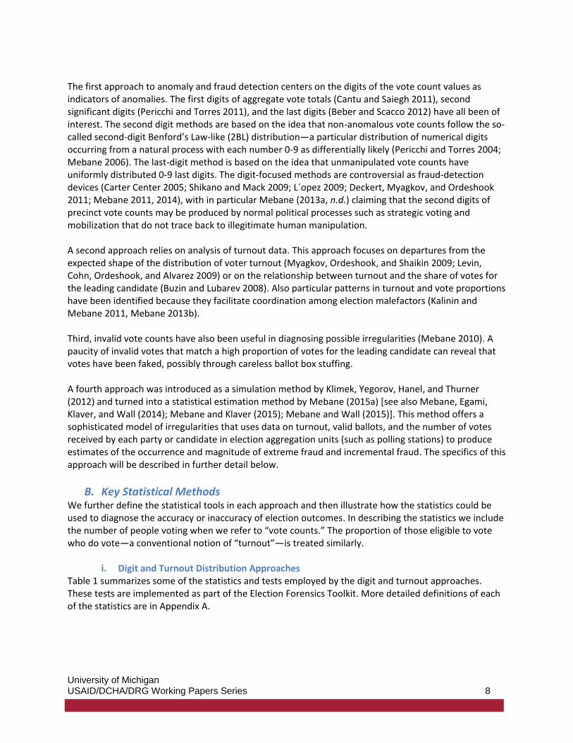
Figures 9 and 10 show there is significant geographic clustering in the vote percentage 0-5 indicator variable no matter whether it is computed using vote percentages for the BNP or for the Awami League. Interestingly, many areas where there are clusters of significantly high values for one party are also areas where there are clusters of significantly high values for the other party (for example, in areas in the northwest). Likewise, many areas with clusters of significantly low values are the same for both parties (to the east). In the central part of the country, we see a few overlaps between areas with clusters of significantly high frauds probabilities and clusters of high averages of the indicator variable. Clusters for the BNP percentage indicator variable (Figure 9) overlap with a few of the high incremental fraud clusters (Figure 8; in the middle) but not so much the high extreme fraud clusters. Clusters for the Awami League indicator variable (Figure 10) overlap with a few of the high extreme fraud clusters (Figure 7; in the north, in the middle, and to the south) and with a few of the high incremental fraud clusters (in the middle).

University of Michigan USAID/DCHA/DRG Working Papers Series 26

Figure 9: Hotspot Analysis, Percentage 0-5 Indicator, Bangladesh 2001, BNP

Note: rounded percentage last-digit 0/5 significant digit union average hotspot analysis using Getis-Ord Gi.

University of Michigan USAID/DCHA/DRG Working Papers Series 27

Figure 10: Hotspot Analysis, Percentage 0-5 Indicator, Bangladesh 2001, Awami League

Note: rounded percentage last-digit 0/5 significant digit union average hotspot analysis using Getis-Ord Gi.

For the other variables that are based on the last digits of the vote counts, significant geographic

clusters are only sporadically observed—a few with significantly high values and a few with

significantly low values. In a couple of instances, the clusters for these variables overlap with

clusters of significantly high values for the frauds probabilities, but on the whole they do not add

University of Michigan USAID/DCHA/DRG Working Papers Series 28

appreciable information to what the clusters, based on the vote percentage indicator variables,

convey.21

The second significant digits of the vote counts exhibit slightly more extensive clustering than do the

vote counts’ last digits, but much less than the vote percentage indicator variables. See Mebane

(2015b) or the Election Forensics Toolkit for figures that show the clustering results for the second

significant digits of the vote counts for the BNP and for the Awami League. For the BNP, only one

cluster of high second-digit values overlaps with a cluster of high incremental fraud probabilities. For

the Awami League, none of the second-digit clusters overlap with a cluster of high frauds

probabilities. The two measures—the frauds probabilities and the second digits—do not appear to

be much related in Bangladesh 2001, at least as far as the properties of their geographic

distributions are concerned. If the frauds probabilities connect to genuine frauds, then the second

digits are not detecting those frauds.

To emphasize the point that the second significant digits of the polling station vote counts probably

are responding strongly to strategic behavior, we consider the conditional distributions produced

when those digits are regressed on margins between the top candidates in each district. This kind of

diagnostic, developed extensively in Mebane (2013a, n.d.), uses non-parametric regressions.22 The

margins of interest are the differences between the proportions of votes for the first-place and

third-place party in each district and the differences between the proportions of votes for the

second-place and third-place party. These margins relate to the proportion of votes for the first- and

second-place parties, respectively, that are being strategically switched by voters who are motivated

by wasted vote logic (Cox 1994, 1997). Roughly speaking, the rationale is that the larger each margin

is, then the more strategic vote switching occurs toward the two parties that are leading in each

district. Mebane (2013a, n.d.) argues that these margins relate to the second significant digits of

low-level vote counts in characteristic patterns.

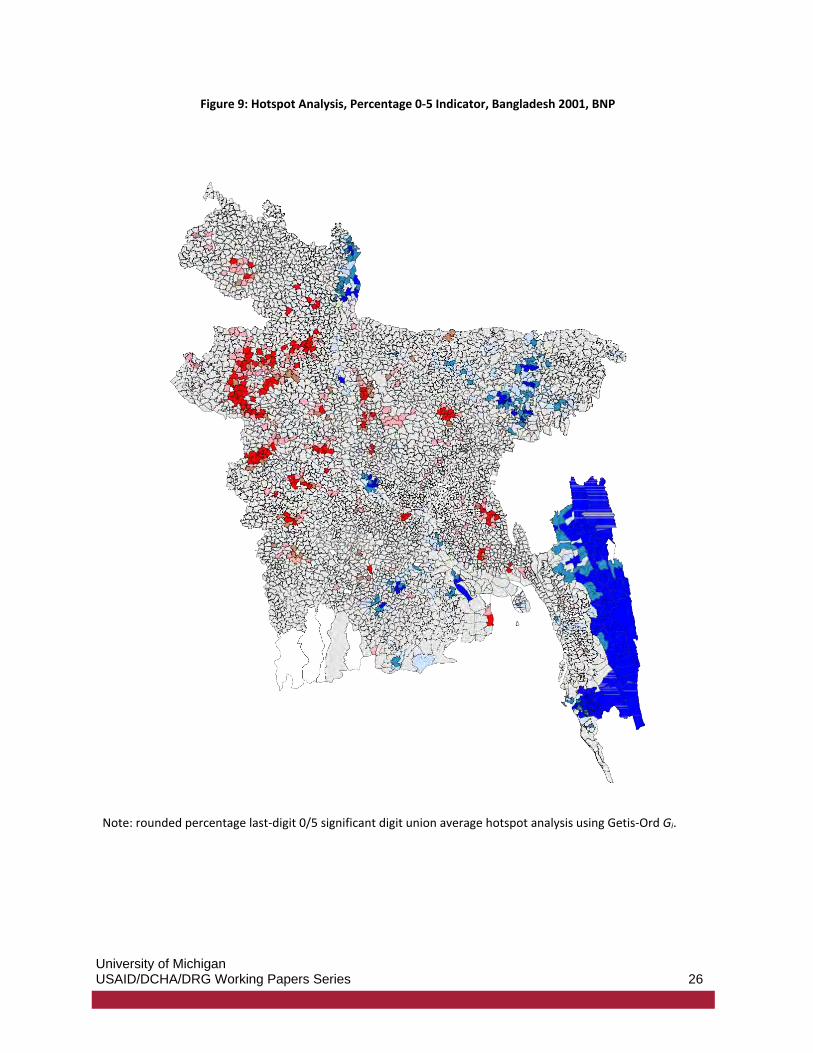
Figure 11 shows patterns that match those typically seen when a certain kind of strategic voting

occurs. In Figure 11(a), the outcome is the second digit in each polling station vote count for the

first-place (winning) candidate in each district. In Figure 11(b), the outcome is the second digit in

each polling station vote count for each district’s second-place candidate. Rug plots along the edges

of each graph show the locations of the margins for each district.

The regressions shown in Figure 11 are two-dimensional non-parametric regressions: both the first-

versus-third and the second-versus-third margins are regressors. The mostly vertical contours of the

conditional mean of the winner’s second digits shown in Figure 11(a) imply that the digit means

depend mainly on the first-versus-third margin, and the mostly horizontal contours of the

conditional mean of the second-place finisher’s second digits shown in Figure 11(b) imply that those

digit means depend mainly on the second-versus-third margin. The conditional mean of the winning

21 The figures that show these clustering results may be viewed via the Election Forensics Toolkit. 22 Non-parametric regressions are computed using the sm package (Bowman and Azzalini 2014, 1997) of R

(R Development Core Team 2005).

University of Michigan USAID/DCHA/DRG Working Papers Series 29

party’s digits is always less than 4.187 and tends to decrease as the first-versus-third margin

increases, as happens in simulations of strategic voting with multiple competitive parties, and then

the mean increases slightly, as it does in data from Canada and Mexico (Mebane 2013a, n.d.). The

conditional mean of the second-place party’s digits is greater than 4.187 for a second-versus-third

margin near zero, then decreases steadily as the margin increases. That is precisely the pattern seen

in simulations with multiple competitive parties when there is no strategic voting (Mebane 2013a,

Figure 2).

Figure 11: Second-Digits Regressed on Inter-Party District Margins, Bangledash 2001

University of Michigan USAID/DCHA/DRG Working Papers Series 30

The pattern in which asymmetric strategic voting occurs—when the winning party appears to attract strategically switched votes but the losing party does not—is one that also occurs in data from Canadian elections (Mebane 2013a, n.d.). Nothing in the analysis in Figure 11 resembles what happens when a fraud based on coercion spanning the whole electorate is simulated (Mebane 2013a, n.d.). “Coercion” could mean any kind of voter intimidation, vote buying, ballot box stuffing, or simply faked votes. The Bangladesh 2001 election was complicated. Both frauds and strategic behavior likely occurred. Frauds occured in some areas: probably genuine fraudulent activities occured in the areas that have significantly high clusters of frauds probabilities; and genuine frauds are especially likely in areas where the frauds probability clusters overlap with the clusters that have high indicators for the occurrence of zeros and fives in the parties’ rounded percentages. Our methods currently do not allow us to estimate the magnitude of the frauds in terms of the number of votes affected. The second significant digits of the polling station vote counts seem not to be much related to the frauds, but they very strongly suggest that a certain kind of strategic voting occurs. The strategic voting pattern is asymmetic: the winning candidate in a district attracts strategically switched votes but the second-place candidate does not. This strategic voting pattern is not compatible with some well-known theories of how wasted vote logic operates, but it is a pattern frequently observed in other countries in which election frauds are routinely believed to be rare and small.

STATUS OF ELECTION FORENSICS METHODS As the examples of South Africa 2014 and Bangladesh 2001 show, when adequate, low-level, aggregate data about an election are available, current election forensics methods allow one to reach extremely precise conclusions about whether and where election frauds occur. Here we have estimated the probability of frauds at individual polling stations. In other cases, where suitable data existed, frauds probabilities have been estimated for individual ballot boxes (Mebane and Wall 2015). Such conclusions are always subject to the caveat that apparent frauds may really be consequences of strategic behavior, but that ambiguity can sometimes be mitigated by exploiting a multiplicity of statistics, as we have attempted to do here (and in Mebane 2015b). An election fraud will not necessarily trigger all of the statistics and tests, but we think a genuine fraud will in general set off many of them. Such reinforcement among diverse statistics and tests has informed the judgments we reach not only here about the elections in South Africa 2014 and Bangladesh 2001 but about elections in the other six countries on which analysis was conducted as part of the work for the grant that has supported this work (Mebane 2015b). Election forensics as a field is at an early stage of its development, but already it is capable of supporting meaningful analysis. The set of methods we have used is not an exhaustive collection of all the methods that have been proposed. New methods continue to be developed and existing methods continue to be better understood. In this Guide, we have illustrated one method for using geographic information to identify frauds, but elsewhere other methods have been considered (Mebane and Kalinin 2014) and many others are certainly conceivable. The core dilemma of trying to distinguish fraudulent from strategic behavior should be a central focus of future research.

University of Michigan USAID/DCHA/DRG Working Papers Series 31

There are also other important areas for further work in election forensics. Perhaps the most important outstanding problem, which we have largely ignored, is to adapt election forensics methods to features of the election system. Existing methods focus on the party or candidate that receives the most votes, sometimes labeling that party the “winner.” But in election systems that use proportional representation, which are prevalent around the world, many parties are “winners” in the sense that many parties gain seats in the legislature as a result of votes cast in the election. Elections in several of our eight countries use proportional representation, but we have not done anything special to exploit or address that. Technology does not exist to do more than look at several of the competing parties, as we have done. Some systems have district magnitudes greater than one with voting rules such as the single-non-transferable-vote, which causes complexities for election forensics. One of our countries, Libya 2014, is a case with such rules. Some of the methods we have described in this Guide do not work in such a system [see Mebane (2015b) for details]. Other electoral systems exist (Taagepera and Shugart 1989, Shugart and Carey 1992, Cox 1997, Powell 2000), presenting a range of settings in which to tune election forensics methods. Different electoral systems present opportunities for a variety of strategic behaviors. The central dilemma that challenges election forensics—distinguishing election fraud from strategic behavior—will persist as we endeavor to develop methods to handle the full diversity of electoral systems.

University of Michigan USAID/DCHA/DRG Working Papers Series 32

REFERENCES Anselin, Luc. 1995. “Local Indicators of Spatial Association—LISA.” Geographical Analysis 27(2):93–115. Beber, Bernd and Alexandra Scacco. 2012. “What the Numbers Say: A Digit-Based Test for Election Fraud.” Political Analysis 20(2):211–234. Benjamini, Yoav and Yosef Hochberg. 1995. “Controlling the False Discovery Rate: A Practical and Powerful Approach to Multiple Testing.” Journal of the Royal Statistical Society, Series B 57(1):289–300. Borghesi, C. and J. P. Bouchaud. 2010. “Spatial Correlations in Vote Statistics: A Diffusive Field Model for Decision-Making.” European Physical Journal B 75(3):395–404. Bowman, A. W. and A. Azzalini. 2014. R package sm: nonparametric smoothing methods (version 2.2-5.4). University of Glasgow, UK and Universit`a di Padova, Italia. http://www.stats.gla.ac.uk/~adrian/sm, http://azzalini.stat.unipd.it/Book_sm Bowman, Adrian W. and Adelchi Azzalini. 1997. Applied Smoothing Techniques for Data Analysis: The Kernel Approach with S-Plus Illustrations. Oxford: Clarendon Press. Buzin, Andrei and Arkadii Lubarev. 2008. Crime Without Punishment: Administrative Technologies of Federal Elections of 2007-2008 (In Russian: Prestupleniye bez nakazaniya. Administrativniye tekhnologii federal’nih viborov 2007-2008 godov). Moscow: Nikkolo M. Callen, Michael, Clark Gibson, Danielle Jung, and James D. Long. 2013. “Reducing Electoral Fraud with Information and Communications Technology in Uganda.” Unpublished manuscript. Callen, Michael and James D. Long. 2013. “Institutional Corruption and Election Fraud: Evidence from a Field Experiment in Afghanistan.” Unpublished manuscript. Callen, Michael, James Long, and Mohammad Isaqzadeh. 2011. “Point and shoot elections.” Foreign Policy: The AfPak Channel. December 15, 2011. http://afpak.foreignpolicy.com/posts/2011/12/15/point_and_shoot_elections. Cantu, Francisco and Sebastian M. Saiegh. 2011. “Fraudulent Democracy? An Analysis of Argentina’s Infamous Decade Using Supervised Machine Learning.” Political Analysis 19(4):409–433. Canty, Angelo and Brian Ripley. 2015. “boot: Bootstrap R (S-Plus) Functions.” R package version 1.3-17. Carter Center. 2005. “Observing the Venezuela Presidential Recall Referendum: Comprehensive Report.” Centre for Research and Information. 2002. A Rigged Election: An Illegitimate Government: Bangladesh Election 2001. Dhanmondi: Centre for Research and Information.

University of Michigan USAID/DCHA/DRG Working Papers Series 33

Cox, Gary W. 1994. “Strategic Voting Equilibria Under the Single Nontransferable Vote.” American Political Science Review 88:608–621. Cox, Gary W. 1997. Making Votes Count: Strategic Coordination in the World’s Electoral Systems. New York: Cambridge University Press. Dahl, Robert. 1971. Polyarchy: Participation and Opposition. New Haven: Yale University Press. Davison, A. C. and D. V. Hinkley. 1997. Bootstrap Methods and their Application. New York: Cambridge University Press. Deckert, Joseph, Mikhail Myagkov, and Peter C. Ordeshook. 2011. “Benford’s Law and the Detection of Election Fraud.” Political Analysis 19(3):245–268. European Union. 2001.“Preliminary Statement—2 October 2001.” European Union– Election Observation Mission in Bangladesh 2001. Getis, Arthur and J. K. Ord. 1992. “The Analysis of Spatial Association by Use of Distance Statistics.” Geographical Analysis 24(3):189–206. Hartigan, J. A. and P. M. Hartigan. 1985. “The Dip Test of Unimodality.” Annals of Statistics 13:70–84. Hyde, Susan D. 2011. The Pseudo-Democrats Dilemma: Why Election Observation Became an International Norm. Ithaca, NY: Cornell University Press. Kalinin, Kirill and Walter R. Mebane, Jr. 2011. “Understanding Electoral Frauds through Evolution of Russian Federalism: from ‘Bargaining Loyalty’ to ‘Signaling Loyalty’.” Paper presented at the 2011 Annual Meeting of the Midwest Political Science Association, Chicago, IL, March 31–April 2. Kelley, Judith. 2012. Monitoring Democracy: When International Election Observation Works and Why it Often Fails. Princeton: Princeton University Press. Kelley, Judith and Kiril Kolev. 2010. “Election Quality and International Observation 1975-2004: Two New Datasets.” October 19, 2010. Available at SSRN: http://ssrn.com/abstract=1694654. Klimek, Peter, Yuri Yegorov, Rudolf Hanel, and Stefan Thurner. 2012. “Statistical Detection of Systematic Election Irregularities.” Proceedings of the National Academy of Sciences 109:16469–16473. Levin, Ines, Gabe A. Cohn, Peter C. Ordeshook and R. Michael Alvarez. 2009. “Detecting Voter Fraud in an Electronic Voting Context: An Analysis of the Unlimited Reelection Vote in Venezuela.” 2009 Electronic Voting Technology Workshop/Workshop on Trustworthy Elections, Montreal, August 10–11, http://www.usenix.org/event/ evtwote09/tech/full_papers/levin.pdf. Lindberg, Staffan. 2006. Democracy and Elections in Africa. Baltimore, MD: Johns Hopkins University Press.

University of Michigan USAID/DCHA/DRG Working Papers Series 34

Lopez, Jorge Alberto Gallardo. 2009. 2006 ¿Fraude Electoral? Chihuahua, Mexico: Doble H´elice Ediciones. Maechler, Martin. 2013. diptest: Hartigan’s dip test statistic for unimodality - corrected code. R package version 0.75-5. http://CRAN.R-project.org/package=diptest Mebane, Jr., Walter R. 2006. “Election Forensics: Vote Counts and Benford’s Law.” Paper prepared for the 2006 Summer Meeting of the Political Methodology Society, UC Davis, July 20–22. Mebane, Jr., Walter R. 2008. Election Forensics: The Second-Digit Benford’s Law Test and Recent American Presidential Elections. In The Art and Science of Studying Election Fraud: Detection, Prevention, and Consequences, ed. R. Michael Alvarez, Thad E. Hall and Susan D. Hyde. Washington, DC: Brookings Institution pp. 162–181. Mebane, Jr., Walter R. 2010. “Fraud in the 2009 Presidential Election in Iran?” Chance 23:6–15. Mebane, Jr., Walter R. 2011. “Comment on ‘Benford’s Law and the Detection of Election Fraud’.” Political Analysis 19(3):269–272. Mebane, Jr., Walter R. 2013a. “Election Forensics: The Meanings of Precinct Vote Counts’ Second Digits.” Paper presented at the 2013 Summer Meeting of the Political Methodology Society, University of Virginia, July 18–20, 2013. Mebane, Jr., Walter R. 2013b. “Using Randomization and Vote Counts’ Digits to Diagnose Election Frauds: Russia.” Paper presented at the 2013 Annual Meeting of the American Political Science Association, Chicago, August 29–September 1, 2013. Mebane, Jr., Walter R. 2014. Can Votes Counts’ Digits and Benford’s Law Diagnose Elections? In The Theory and Applications of Benford’s Law, ed. Steven J. Miller. Princeton: Princeton University Press pp. 206–216. Mebane, Jr., Walter R. 2015a. “Election Forensics: Latent Dimensions of Election Frauds and Strategic Voting.” Paper presented at the 2015 Summer Meeting of the Political Methodology Society, Rochester, July 23–25. Mebane, Jr., Walter R. 2015b. “Election Forensics Toolkit DRG Center Working Paper.” Working paper for subaward #DFG-10-APS-UM. Mebane, Jr., Walter R. n.d. “Election Forensics.” book MS. Mebane, Jr., Walter R. and Jonathan Wall. 2015. “Election Frauds, Postelection Legal Challenges and Geography in Mexico.” Paper presented at the 2015 Annual Meeting of the American Political Science Association, San Francisco, CA, September 3–6.

University of Michigan USAID/DCHA/DRG Working Papers Series 35

Mebane, Jr., Walter R. and Joseph Klaver. 2015. “Election Forensics: Strategies versus Election Frauds in Germany.” Paper presented at the 2015 Annual Conference of the European Political Science Association, Vienna, Austria, June 25–27, 2015. Mebane, Jr., Walter R. and Kirill Kalinin. 2009a. “Comparative Election Fraud Detection.” Paper prepared for the 2009 Annual Meeting of the Midwest Political Science Association, Chicago, IL, April 2–5. Mebane, Jr., Walter R. and Kirill Kalinin. 2009b. “Electoral Falsification in Russia: Complex Diagnostics Selections 2003-2004, 2007-2008 (in Russian).” Electoral Policy REO /09:57–70. Mebane, Jr., Walter R. and Kirill Kalinin. 2014. “Geography in Election Forensics.” Paper presented at the 2014 Annual Meeting of the American Political Science Association, Washington, DC, August 28–31. Mebane, Jr., Walter R., Naoki Egami, Joseph Klaver and Jonathan Wall. 2014. “Positive Empirical Models of Election Fraud (that May Also Measure Voters’ Strategic Behavior.” Paper presented at the 2014 Summer Meeting of the Political Methodology Society, University of Georgia, July 24–26, 2014. Myagkov, Mikhail, Peter C. Ordeshook, and Dimitry Shaikin. 2009. The Forensics of Election Fraud: With Applications to Russia and Ukraine. New York: Cambridge University Press. Ord, J. K. and Arthur Getis. 1995. “Local Spatial Autocorrelation Statistics: Distributional Issues and an Application.” Geographical Analysis 27(4):286–306. Pericchi, Luis Raul and David Torres. 2004. “La Ley de Newcomb-Benford y sus aplicaciones al Referendum Revocatorio en Venezuela.” Reporte Tecnico no-definitivo 2a. version: Octubre 01, 2004. Pericchi, Luis Raul and David Torres. 2011. “Quick Anomaly Detection by the Newcomb-Benford Law, with Applications to Electoral Processes Data from the USA, Puerto Rico, and Venezuela.” Statistical Science 26(4):502–516. Powell, Bingham. 2000. Elections as Instruments of Democracy. New York: Yale University Press. R Development Core Team. 2005. R: A Language and Environment for Statistical Computing. Vienna, Austria: R Foundation for Statistical Computing. ISBN 3-900051-07-0. http://www.R-project.org Rundlett, Ashlea and Milan W. Svolik. 2015. “Deliver the Vote! Micromotives and Macrobehavior in Electoral Fraud.” Working paper. Shikano, Susumu and Verena Mack. 2009. “When Does the Second-Digit Benford’s Law Test Signal an Election Fraud? Facts or Misleading Test Results.” Jahrbu¨cher fur National¨okonomie und Statistik 231(5-6):719–732. Shpilkin, Sergey. 2011. “Statistika issledovala vybory: Statisticheskij analiz vyborov v Gosdumu 2011 goda pokazyvaet vozmozhnye fal’sifikacii (Statistics examined elections: Statistical analysis of elections to the State Duma in 2011 shows possible fraud).” gazeta.ru (in Russian), http://www.gazeta.ru/science/2011/12/10_a_3922390.shtml , December 10, 2011.

University of Michigan USAID/DCHA/DRG Working Papers Series 36

Shugart, Matthew Soberg and John M. Carey. 1992. Presidents and Assemblies: Constitutional Design and Electoral Dynamics. New York: Cambridge University Press. Taagepera, Rein and Matthew Soberg Shugart. 1989. Seats and Votes: The Effects and Determinants of Election Systems. New York: Yale University Press. Zakaria, Fareed. 1997. “The Rise of Illiberal Democracy.” Foreign Affairs 76(6):249–295.

University of Michigan USAID/DCHA/DRG Working Papers Series 37

APPENDIX A: DIGIT AND DISTRIBUTION APPROACHES 2BL: second-digit mean. “Second-digit” refers to the second significant digit in each count to which the test is applied (for example, if the count is “1234,” then “2” is the second significant digit). Pericchi and Torres (2011) argue that if vote counts are produced in an unproblematic election, then the distribution of the second digits should be approximately that implied by Benford’s Law. The frequency with each digit occurs as the second significant digit according to Benford’s Law is shown in Table 4. In fact the digits in vote counts do not have the distribution implied by Benford’s Law, even though the second digits often do, a situation Mebane (2006, 2008) describes by referring to “second-digit Benford’s Law-like” (or 2BL) distributions. Pericchi and Torres 2011 argue that a kind of chi-square statistic applied to the distribution of the second digits of vote counts can detect election frauds, but many have expressed doubt about the efficacy of second digits as fraud detectors (Carter Center 2005; Shikano and Mack 2009; Lopez 2009; Cantu and Saiegh 2011; Deckert, Myagkov, and Ordeshook 2011; Mebane 2011). If the second digits occur with the frequencies given in Table 4, then their mean is 4.187 = ∑9

j=0 jrj ≡ 𝑗 ̅where rj is the frequency for digit j. While frauds may cause the digits in vote counts not to have a 2BL distribution, Mebane (2013a, 2014, n.d.) shows that the second digits also respond strongly and with regular patterns both to the way voters are grouped into aggregation units (for example, by gerrymandering) and to strategic behavior by voters (such as strategic voting). Conditional means (denoted 𝑗̂x) produced by non-parametrically regressing the second digits on “x” variables such as the margins between candidates in each election district are needed to use the second digits to help diagnose whether frauds or strategies or both are occurring in an election. Value expected in the absence of frauds or strategic behavior: 2BL = 4.187.

Table 4: Frequency of Second Digits according to Benford’s Law

digit 0 1 2 3 4 5 6 7 8 9

probability .120 .114 .109 .104 .100 .097 .093 .090 .088 .085

LastC: last-digit mean. “Last-digit” refers to the last digit in each count to which the test is applied (for example, if the count is “1234,” then “4” is the last digit). Beber and Scacco (2012) argue that if vote counts are produced in an unproblematic election, then the distribution of the last digits should be uniform, which is to say that each of the ten digits (0, 1, 2, 3, 4, 5, 6, 7, 8, 9) should occur with frequency 1/10. If the last digits occur with such frequencies, then their mean is 4.5 = ∑9

j=0 j. Beber and Scacco (2012) exclude counts less than 100 when assessing the last digit distributions. Using data from Russian elections, Mebane (2013b) shows that the last digits can appear to have a uniform distribution even when substantial election frauds can be demonstrated by other means—in such cases, the digits are likely faked. But such fakery requires near total control over the reported results. Value expected in the absence of frauds or strategic behavior: LastC = 4.5. C05s: mean of a binary variable indicating whether the last digit of vote count for the referent party or candidate is zero or five. As a special case of the Beber and Scacco (2012) argument, the expected value for the mean of this indicator variable in the absence of frauds is C05s = 0.2.

University of Michigan USAID/DCHA/DRG Working Papers Series 38

P05s: mean of a binary variable indicating whether the last digit of the rounded percentage of votes for the referent party or candidate is zero or five. If agents need to signal that they have committed fraudulent acts, then these digits may be especially likely to appear, as has been amply demonstrated to occur in Russian elections (Mebane and Kalinin 2009a,b; Kalinin and Mebane 2011; Shpilkin 2011; Mebane 2013b; Rundlett and Svolik 2015). A mean for the variable that indicates whether the rounded percentages end in zero or five that is larger than 0.2 suggests such a signal-related manipulation. Value expected in the absence of frauds or strategic behavior: P05s = 0.2. DipT: test of unimodality. Motivation for the test of unimodality comes from the argument that multimodality (multiple distinct peaks) in the distribution of turnout proportions indicates irregularities (Myagkov, Ordeshook, and Shaikin 2009; Levin et al. 2009). A theoretical argument about the dynamic process in which collective choices occur also asserts that, under a wide range of conditions, distributions not only of turnout but of winners’ vote shares should be unimodal (Borghesi and Bouchaud 2010). The test is from Hartigan and Hartigan (1985). The statistic is the p-value for a null hypothesis that the distribution is unimodal. Very small p-values give reason to reject the hypothesis. Value expected in the absence of frauds or strategic behavior: DipT > .05. Skew: skewness. If arguments against multimodality are sharpened into an argument that the distribution of turnout proportions should be Normal, then skewness should be zero. A Normal distribution is symmetric. Skewness is a measure of asymmetry. A symmetric distribution, and in particular the Normal distribution, has skewness zero. If skewness is significantly different from zero, there may be problems with the election. Klimek et al. (2012) point out that skewness alone is not necesarily an indicator for election frauds, but significant non-zero skewness along with other indicators (such as kurtosis) can suggest that frauds occurred (positive or negative skewness). Value expected in the absence of frauds or strategic behavior: Skew = 0. Kurt: kurtosis. If arguments against multimodality are sharpened into an argument that the distribution of turnout proportions should be Normal, then kurtosis should be three. Kurtosis measures the rate at which the frequency of values that differ from the mean declines as values more and more distant from the mean are considered. A Normal distribution has kurtosis equal to three. If kurtosis is significantly different from three, there may be problems with the election. Klimek et al. (2012) point out that kurtosis alone is not necesarily an indicator for election frauds, but kurtosis significantly different from three along with other indicators (such as skewness) can suggest that frauds occurred (excess kurtosis). Value expected in the absence of frauds or strategic behavior: Kurt = 3.