NOAA Technical Report ERL 384-PMEL 27

A General Modelof the Ocean Mixed LayerUsing a Two-Component Turbulent Kinetic EnergyBudget with Mean Turbulent Field Closure

Roland W. Garwood, Jr.

Pacific Marine Environmental LaboratorySeattle, Washington

September 1976

U.S. DEPARTMENT OF COMMERCEElliot Richardson. Secretary

National Oceanic and Atmospheric Administration

Robert M. White. Administrator

Environmental Research Laboratories

Wilmot Hess. DirectorBoulder. Colorado

Adapted from a dissertationsubmitted to the University of Washington

in partial fulfillment ofthe requirements for the degree of

Doctor of Philosophy

i i

CONTENTS

PAGE

3. CLOSING THE PROBLEM

2. REVIEW OF THE LITERATURE

4. ENTRAINMENT HYPOTHESIS

5. BEHAVIOR OF THE EQUATIONS

v

434648

49

1

1

157

15

16

1617181821

232629

33

34343536

36

363841

Ekman Depth of Frictional ResistanceRossby NumberEddy Transfer Coefficients in a Steady-State ProblemObukhov Length ScaleCompensation Depth for Shortwave RadiationPrototype Turbulent-Energy-Budget Model:Kraus and Turner

Adding DissipationRole of Mean Kinetic Energy

Entrainment in Earlier Mixed Layer ModelsSuggested Turbulent MechanismRelevant Parameters and a Dimensional AnalysisTurbulent Kinetic Energy Budget at the Density Interface

and the Development of a Theoretical Equation for Turbu­lent Entrainment in the Presence of Mean Shear

Comparison with Moore and Long (1971) ExperimentCompleted Model for Shallow Mixed Layers

Net Viscous Dissipation in the Mixed LayerNet Effect of Redistribution of Turbulent EnergyShear ProductionNeed for an Entrainment Equation

1.1. Purpose of the Study1.2. Characteristics of the Ocean Mixed Layer1.3. Fundamental Principles and Equations1.4. Course of Action in Attacking the Problem

4.5.4.6.

3.l.3.2.3.3.3.4 .

2.l.2.2.2.3.2.4.2.5.2.6.

2.7.2.8.

4.l.4.2.4.3.4.4.

NOTATION

ABSTRACT

1. INTRODUCTION

5.1. Nondimensional Form of the Turbulent Energy andEntrainment Equations

5.2. Determination of the Constants5.3. Comparison with Earlier Models

495052

iii

6. DEEP MIXED LAYERS: LIMIT TO MAXIMUM DEPTH

7. CONCLUS IONS

8. SUMMARY OF MODELED EQUATIONS

9. ACKNOWLEDGMENTS

10. REFERENCES

6.l.6.2.6.3.

6.4.

6.5.

6.6.6.7.

Limiting Dissipation Time ScaleNondimensional Solution to the Entrainment FunctionSimple Hypothetical Cases Demonstrating the Behaviorof the Solution

6.3.1. Shallow or f ~ 0 (Ro » 1)6.3.2. Convective planetary boundary layer with order

one Rossby numberFiltering Effect of the Storage of Turbulent KineticEnergy

Interaction Between Forcing Time Scales: Modulationof the Longer-Period Trend by the Diurnal-PeriodHeating/Cooling Cycle

Simulation of a Real CaseEvaluation of Model Output

54

5456

60

60

65

68

707174

75

77

78

79

iv

()

< >-b = B + b*B

bw

cw

Cp

CD

C = U+ iV

c = u + iv

d

d'

D

Ds

lE 1 u2 + v2 + w2= 2Ui ui =2 2

*E

* * *Ell + E22 + E33

NOTATION

The horizontal mean (often justcapitalized: ~ = T, etc.)

The vertical mean over the mixed layer

Buoyancy

Parameter for relative importance ofH* to RO-l for cyclical steady state

Turbulent buoyancy flux

Complex turbulent momentum flux

Specific heat at constant pressure

Drag coefficient in quadratic windstress law

Mean horizontal velocity in complex form

Turbulent horizontal velocity in complexform

Ekman depth of frictional resistance

Surface production zone (Niiler); alsoused as a depth proportional to Ekmandepth (d)

Total rate of viscous dissipation ofturbulent kinetic energy in themixed layer

Molecular diffusion coefficient

Turbulent kinetic energy (per unit mass)

-<E>/(htlB)

Turbulent kinetic energy nondimension­alized with the friction velocitysquared, u~

Coriolis parameter

v

F

g

G

h

*H

K = Km

KT

L

m. , p., ,n

N

p

Damping force for inertial motions

Apparent gravitational acceleration

Total rate of mechanical productionof turbulent kinetic energy in themixed layer

Depth of mixed layer

Mixed layer depth if the verticalextent of the region is stationaryor retrea ti ng

Mixed layer depth (h) non-dimension­alized with the Obukhov length

Compensation depth for radiative heating

Mechanical equivalent of heat,

24.186 X 107 gm cm

cal sec 2

Eddy mixing coefficient for neutralconditions

Eddy viscosity

Eddy conductivity

Obukhov length scale

Integral turbulence length scale

Convective length scale

Rotational length scale

Model constants

Value for integrated flux Richardsonnumber

Brunt-Vaisala frequency

Fluctuating pressure component

Geostrophic pressure gradient in theocean

vi

PE+ KE

*P

Q

QI

Qo

~ q2 U2 + V2= 2

r

Ro

Ri

RF

*Ri

s = S + s

t

Total mechanical energy per unit massin the mixed layer

Nondimensional entrainment flux

Radiation absorption

Solar heating function

Solar radiation through interface(incident minus reflected)

Horizontal component of turbulentkinetic energy

Fraction of net production going topotential energy by means ofentrainment

Rossby number

Gradient Richardson number,

Flux Richardson number,

- _. aU - aV- bw/ (uw - + vw -). az az

Gradient Richardson number in theentrainment zone

Overall or bulk Richardson number,

hl:lB/ll:ICl2

Total Gradient Richardson number

ab/az=(au/az)2

Sal inity

Time

vii

(u.) = (U+u, V+v, W+W)1

*u

W

*W

(Xi) + (x,y,z)

ex

y( z)

r

oCo

liB

Total instantaneous velocity, the sumof the mean and turbulent components(neglecting any geostrophic com­ponent)

Geostrophic components of velocity

dh/dt, entrainment velocity

Friction velocity, v'!cw(o)I

Surface buoyancy flux, -bw(o)

Wind velocity; sometimes used as meanvertical water velocity

Nondimensional entrainment velocity,

u /..J.E:e

Rectangular space coordinates withx3 = z aligned vertically upward,parallel to the local apparentdirection of gravity

- po-lap/as

Coefficient of thermal expansion,

Extinction coefficient for net solarradiation

aB/al for l < (-h-o) = N2

aT/al for l < (-h-o)

Fraction of turbulent energy dissipated

Thickness of entrainment zone

Excess surface velocity, C(z=o) - <C>

Change in mean buoyancy, across theentrainment zone, B(-h) - B(-h-o)

viii

£

- ik{x - c t)n = noe 1

6 = T + 6

*6

K

A

v

P

ItI

T£

*T

Mean velocity drop across the densityinterface

Rate of viscous dissipation of tur­bulent kinetic energy,

Internal wave amplitude on interface

Temperature

*Temperature flux scale, b lag

Thermal conductivity

Heaviside unit step function; alsoused as dissipation length scale

Molecular viscosity

Kinematic viscosity

The instantaneous density of the seawater

The density for representative valuesof salinity, so' and temperature, 6 0

Representative density of air

Turbulent heat flux

Surface stress, Po u~

Dissipation time scale

Dimensionless time scale, tiT£

T"ime constant for dampi ng by F

Latitude

ix

Q.J

w

E*/Ri* = <E> I~C~(h~B)2

Nondimensionalized turbulent kinetic- 3energy, h<E> / (u* T )

E

Earth's rotation vector

Angular frequency

x

A GENERAL MODEL OF THE OCEAN MIXED LAYERUSING A TWO-COMPONENT TURBULENT KINETIC ENERGY

BUDGET WITH MEAN TURBULENT FIELD CLOSURE

Roland W. Garwood, Jr.

A non-stationary, one-dimensional bulk model of a mixed layerbounded by a free surface above and a stable nonturbulent regionbelow is derived. The vertical and horizontal components of turbu­lent kinetic energy are determined implicitly, along with layerdepth, mean momentum, and mean buoyancy. Both layer growth by en­trainment and layer retreat in the event of a collapse of the ver­tical motions due to buoyant damping and dissipation are predicted.Specific features of the turbulent energy budget include mean tur­bulent field model ing of the dissipation term, the energy redistri­bution terms, and the term for the convergence of buoyancy flux atthe stable interface (making possible entrainment). An entrainmenthypothesis dependent upon the relative distribution of turbulentenergy between horizontal and vertical components permits a moregeneral application of the model and presents a plausible mechanismfor layer retreat with increasing stability. A limiting dissipationtime scale in conjunction with this entrainment equation results ina realistic cyclical steady-state for annual evolution of the upper­ocean density field. Several hypothetical examples are solved, anda real case is approximated to demonstrate this response. Of par­ticular significance is the modulation of longer-period trends 'bythe diurnal-period heating/cooling cycle.

1. INTRODUCTION

1.1 Purpose of the Study

The objective of this study is the formulation of a unified mathematicalmodel of the one-dimensional, nonstationary oceanic turbulent boundary layer.In particular,'this model should help explain and predict the development intime of the seasonal pycnocline.

Interest in the ocean mixed layer stems from both theoretical and prac­tical considerations. Thermal energy and mechanical energy received from theatmosphere not only control the local dynamics, but the layer itself modu­lates the flux of this energy to the deeper water masses. Conversely, fluxof heat back to the atmospheric boundary layer has an important influenceupon the climate and its fluctuations. Figure 1 depicts the mechanicalenergy budget for the ocean mixed layer.

Stable, Neg!.Ver t. Flux

:J EntrainmentZone

MixedLayer

iifIIIlIl-

lI/ bw (0)

~~~~IB=Po-PgPo

SurfaceBuoyancy Flux

U( V)

Work byWind Stress

zT=PU;+ ----+-

MEAN K.E.o

1J(U2+V2)dZ-h-8

nShear

Production

lJ

P. E.oJBzdz

-h'-B'

1I1lInterior

BUO~rl

EntrainmentBuoy. Flux

*

HORIZONTALTURB. K.E

otJ u

2+v 2 dz

-h

*Rp.distribution

c:=====:>

VERTICALTURB. K.E.

oIJ-2' w2 dz-h

~ O;SS;pal;On' 1/~.------.

HEAT* Modeled Processes

F-igU!l.e. 1. Me.c.haniea1. e.n.vz.gy bu.dge.t noJr.. :the. oee.an. mixe.d i..ayvz..

2

In addition to climatological and ocean circulation studies, otherapplications of a practical model of the mixed layer include investigationsof advection and turbulent dilution of dissolved or suspended concentrationsof matter such as pollutants and nutrients. Prediction of entrainment of thedeeper, nutrient-rich water into the mixed layer has particular pertinence tothe estimation of primary productivity.

The need to further develop and attempt to improve the one-dimensionalmixed-layer model is evident. The failure of earlier models to consistentlyexplain the annual cycle of thermocline development is, for the most part,not attributable to the assumption of one-dimensionality.

A refined treatment of the often neglected terms of the turbulent kin­etic energy budget promises to improve the physical understanding of theturbulent ocean boundary layer and make possible the creation of a better­performing model.

A detailed review of the literature associated with mixed-layer modelingis undertaken in Chapter II, but Table 1 summarizes the major historicalcontributions to the understanding of the physics of the mixed layer.

The works of primary concern here are those dealing explicitly withequations for the production, alteration, and destruction of turbulent kin­etic energy within the mixed layer. Kraus and Turner (1967) were the firstto heed the turbulent kinetic energy budget in a one-dimensional mixed layermodel, utilizing the approximately decoupled state of the equations for thethermal and mechanical energies. By neglect of the frictional generation ofheat, the vertically integrated heat equation becomes a relationship for theconservation of potential energy. However, viscous dissipation cannot beneglected in the turbulent energy budget, and Geisler and Kraus (1969) aswell as Miropol'skiy (1970) and Denman (1973) added it to the basic model.Niiler (1975) showed that in addition to the equations for thermal (poten­tial) and turbulent (kinetic) energy, an equation for the mean kinetic energyshould properly be incorporated because entrainment converts some of the meanflow energy into turbulent energy, over and above the parameterized wind­stress production.

Further questions remain and limit the general applications of theseearlier models:

a. The viscous dissipation of turbulent energy has been parameterizedas a fixed fraction of the wind-stress production and hence is a function ofthe surface friction velocity u*. Dissipation may be related to the integralvelocity scale of the turbulence, but this scale is not always proportionalto u*. Surface heat (buoyancy) flux and entrainment fluxes can contributesignificantly to the turbulent intensity.

b. Entrainment may also be considered a function of the ambient turbu-lence parameters. Instabilities leading to entrainment are probably induced •by horizontal turbulent velocities locally at the bottom of the mixed layer,so the entrainment rate doesn't necessarily correspond to an integral con-straint upon the total turbulent energy budget.

3

Ta.ble. 1. SwnmaJLy 06 H..L6:toJUc.a.i ContJUbution6

Date

1905

1935

1948

Author(s)

Ekman

Rossby andMontgomery

Munk andAnderson

Contribution

Constant eddy viscosity solution to steady-state momentumequation: Ekman ~l; "depth of frictional influence";suggested h ~ Wllsin-~ •

Improved current measurements to demonstrate h ~ u*/f(Rossby number ~ constant).

Simultaneous solution of steady-state heat and momentum equa­tions using eddy mixing coefficients variable with Richardsonnumber.

1960 Kitaigorodsky Using dimensional analysis, suggested that hlength scale.

L, the' Obukhov

1961

1967

1969

1970

1973

1974

Kraus andRooth

Kraus andTurner

Geislerand Kraus

Miropol'skiy;Denman

Pollard, Rhinesand Thompson

Ni i ler

Penetration of solar radiation to depth makes steady-statepossible for heat equation because of surface heat loss byconduction, evaporation, and long wave radiation; unstabledensity profile above compensation depth (hc ) is source ofturbulent kinetic energy produced by convection.

Included mechanical stirring (parameterized in terms of windstress) as well as convective production as important sourceof turbulence for mixing: turbulent kinetic energy equationand heat equation form two-equation model in two unknowns--T,h; non-steady-state solutions and "retreating" (h) possible;viscous dissipation neglected.

First "slab" model in which momentum equation is solved to­_gether with turbulent energy equation and heat equation; layerassumed homogeneous in T and U, V and hence moves as a slab;assumed buoyancy flux is fixed portion of mechanical produc­tion--essentially same as Kraus and Turner; applied model toatmosphere with subsidence.

Assumed dissipation a fixed fraction of mechanical production;remaining turbulent kinetic energy goes to buoyancy flux down­wards including entrainment; essentially same as Kraus andTurner.

Slab model applied to ocean mixed layers; used total mechan­ical energy equation (rather than turbulent equation) plusmomentum and heat equations; h, T, U, V--all functions oftime. Ignored effects of turbulent energy budget altogether.

Re-emphasized the need to use the turbulent kinetic energybudget apart from the total mechanical energy budget; dividedregion into three sub-regions with no mechanical productionin most of the mixed layer. Included turbulent kineticenergy'produced by entrainment of zero-velocity water intomoving slab, but surface mechanical production minus dissi­pation still parameterized in terms of u~. Dissipation isnot affected by the additional entrainment production, pos­sibly causing a too-large entrainment rate.

4

c. The use of the total turbulent energy equation and consequently theneglect of energy redistribution among components also results in a somewhatinconsistent method of predicting layer "retreat." The consideration ofseparate budgets for the horizontal and vertical turbulent energy componentswill permit a more consistent interpretation of both entraining and retreat­ing mixed layers.

In this paper, ad hoc mean turbulent field modeling of the terms in theturbulent kinetic energy equations permits the inclusion of these oftensalient effects in a generalized one-dimensional model of the ocean mixedlayer.

2. CHARACTERISTICS OF THE OCEAN MIXED LAYER

The ocean mixed layer is defined as that fully-turbulent region of theupper ocean bounded on top by the sea-air interface. The wind and intermit­tent upward buoyancy flux attributable to surface cooling are the primarysources of mechanical energy for the mixing.

The most distinctive feature of this layer and what really defines itsextent is its relatively high intensity of continuous, three-dimensionalturbulent motion. Vertical turbulent fluxes within the mixed layer can be somuch greater than vertical fluxes in the underlying stable water column thatthe dynamics of the layer are essentially decoupled from the underlyingregion. (Of course the dynamics of the underlying water masses are probablyvery dependent upon the mixed layer.)

Typically, an actively entraining mixed layer is bounded on th~ bottomby a sharp density discontinuity separating the layer from a stable, essen­tially nonturbulent thermocline. Minimal stress at the bottom together withhigh turbulence intensity results in an approximate vertical uniformity inmean velocity and density. This ostensible homogeneity is the root of theterm "sl ab," often used to describe the layer. On the other hand, only smallgradients in these mean variables give rise to large turbulent fluxes. There­fore, even the slight non-homogeneity is highly important in the physics ofthe region and should not be neglectea at the outset.

The nearly zero-flux state of the underlying thermocline causes thebottom boundary condition of the mixed layer to act almost as a slip condi­tion on the mean velocity. This in turn creates a trap for inertial motion.

Deepening of the mixed layer is accomplished by entrainment of the more­dense underlying water into the turbulent region above. This process entailsa potential energy increase and cannot take place without an energy source-­the turbulent kinetic energy of the mixed layer above.

A simplified picture of the region is shown in Figure 2. There is anappealing practical aspect to the judicious use of the assumption of verticalhomogeneity. This assumption permits the use of the vertically integrated

5

z

---+--."....----- P - Po

z -T.-r---+-----<..:...:u:r>--::::;;:;o-- U (V)

-h-h-8

h

18

T

F-<.guJLe 2. Ide.aU.zed model. 60J!. oc.e.aYl mix.ed futje.JL (----1. Mix.ed futje.JL depth-iA rh); (<5) .u. the thic.k.ne6.6 06 the -<.n:te.JL6a.c.e oJ!. enttuLi.nmen:t zone.

momentum and heat (buoyancy) equations, thus avoiding the turbulent flux (ofmomentum and buoyancy) closure problem altogether.

The depth of the oceanic wind-mixed surface layer is typically on theorder of ten to a hundred meters. The horizontal scale size is that of theradius of the circle of inertia--seldom larger than a few kilometers in tem­perate latitudes. These two dominant scale sizes are usually significantlysmaller than the horizontal scale sizes of the driving meteorological distur­bances, water mass features, and distance to lateral boundaries. Therefore,the approximation of local horizontal homogeneity for all mean variables isusually accurate and is a basic assumption of this work. The local conse­quence of some lateral inhomogeneity can be parameterized without qualita­tively undermining such a one-dimensional model. For example, a divergenceof the horizontal current field results in a nonzero vertical mean velocitywhich in itself can be assumed locally uniform in the horizontal. A minorrate of loss (compared with the surface flux) of mean momentum by lateraland/or downward radiation of inertial motion may be parameterized also with­out compromising the dominant processes.

Substantial barotropic and baroclinic features in the mean fields canbe linearly superimposed. The mean fields of concern are therefore the hori­zontally homogeneous components of the total fields. In particular, the

6

momentum equation has the geostrophic component subtracted out, eliminatingany lateral pressure gradient.

1.3 Fundamental Principles and Equations

The underlying principles employed in studying the mixed layer are thecombined conservations of mass, momentum, thermal energy, and mechanicalenergy.

The conservation of momentum and the condition of incompressibility arereflected by the Navier-Stokes equations of motion, invoking the Boussinesqapproximation:

au. au.'+ '" -'+Po~ Po uj ax.

J

--.J.",'" ap au.

Po E. ·kS"LU k +" - (po - ,,)g 0'.3 = l.l ''J J aX,. aX.aX.J J

au.,ax. = 0 .,

(1.1 )

(1. 2)

Because frictional generation of heat is negligible compared with typi­cal magnitudes for the divergence of heat flux, the conservation of thermalenergy is decoupled from the mechanical energy budget, and the first law ofthermodynamics for an incompressible fluid gives the heat equation.

(1. 3)

The conservation of salt mass is of the same form, but it lacks a termanalogous to the radiation absorption term, Q.

(1.4 )

A simplified but sufficiently accurate equation of state for localand reasonably short-term application in the mixed layer is given by

(1.5 )

7

where Po = p(eo,so) is a representative but arbitrary density at the timeand location of consideration. The coefficients (8) and (a) are assumed toremain constant.

Taking the scalar product of (ui) with the respective terms of equation(1.1), the mechanical energy equation is formed,

where the buoyancy (0) is given by

-:v (po-p)o = gPo

'"Vu·1v

'"V4.va u·

1ax.ax. '

J J(1. 6)

(1. 7)

Assuming horizontal homogeneity of mean variables, where the horizontal meanis defined by

x X

en (z,t) = lim L 1212f(x,y,z,t) dxdy ,

x~ x2 -x -x2"" 2""

and separating all variables into mean and fluctuating components gives

Ug + U(z,t) + u(x,y,z,t)

{ui } = Vg + V(z,t) + v(x,y,z,t)

o + w(x,y,z,t)

e = T(z,t) + e(x,y,z,t)

p = \ Pg + p(x,y,z,t),I

0 B(z,t) + b(x,y,z,t)I

= I

I.Strictly speaking, the total fluctuating part of each variable includes

a component directly attributable to surface and internal wave motion. This

8

component has been removed from the fields depicted above. The virtuallyirrotational wave velocities are assumed noninteractive except as an externalsource or sink of turbulent energy due to the net contr"ibutions of breakingsurface waves and radiating internal waves.

In practice, a time mean is employed in data analysis rather than eventhe horizontal mean. Ideally, the averaging time should be short comparedwith the time necessary for significant changes in the mean fields but longcompared with the integral time scale of the turbulence.

--;;::;- 1B(z,t) = (0) ~ 6t Ddt, for example.

In making the Boussinesq approximation, the hydrostatic component ofpressure has already been eliminated. The renlaining mean pressure is assumedto be geostrophic:

(1. 8a)

(1. 8b)

Subtracting the geostrophic equations from the total momentum equationand dropping the negligible viscous terms, the equations for the mean momen­tum become in complex notation (for the sake of brevity)

aC _ ifC acwar-- -az

where C = U + i V and c = u + i v.

(1. 9)

Using equations (1.3), (1.4), (1.5), and (1.7) and again neglectingmolecular fluxes, a buoyancy equation is formed:

(1.10 ) -

9

Equation (1.11) is the mean buoyancy equation.

(1.11)

The use of a buoyancy equation reflecting the combined conservations ofthermal energy and dissolved material is not only more general than a heatequation alone, but it makes more obvious the coupling with the mechanicalenergy budget.

Using the decomposition into mean and fluctuating parts and taking themean of equation (1.6) yields the mean equation for the total mechanicalenergy. Where E = u.u. = u2 + v2 + w2 ,

1 1

+~az

~]ax.J

(1.12 )

The viscous diffusion and viscous dissipation of the mean kinetic energy arenegligible and have been dropped in equation (1.12).

The turbulent kinetic energy equation is formed by subtracting thescalar produce of (Ui) and equation (1.9) from equation (1.12).

1 aE a [~E~ [- aU - avJ r-] []- - + - W 1:- + - + uw - + vw - = bw - £2 at az Po 2 az az . (1. 13)

The budgets for the individual components of turbulent energy areformed in the same manner from equation (1.1) by setting i = 1,2,3 withoutsummation:

(1.14a)

(1.14b)

10

1 aw2 _2" ar- - bw

aaz (

w3

+ ~)2 Po

+ ~ aw + Q2 UW - £3 •Po az (1.14c)

Notice that the orientation of the horizontal axes is (x) positive to theeast and (y) positive to the north~ The rate of viscous dissipationE = v aUiaui/axjaxj beha~es like (E/, E ) and the small size of the dissipationtime constant (lE ~ hill[) compared with the time scale of the meteorologicalforcing causes the intensity of the turbulence to track along in a quasi­steady state with a continually changing net rate of production. Hence thetime rate of change of turbulent kinetic energy is usually much smaller thanthe other terms of (1.13) and thus may be neglected. Because viscous dissi­pation of energy occurs primarily in the range of wave numbers that exhibitlocal isotropy (the equilibrium range), dissipation (E) is divided equallyamong the component budgets (1.14 a-c).

The second term in equation (1.13) is the divergence of the turbulentflux of kinetic energy. Over the whole mixed layer, it probably accounts fora net gain of energy. Wind-wave interactions at the surface result in somenet downward flux, primarily from breaking surface waves. If the Brunt­Vaisala frequency (N) of the adjacent underlying stable water column is suf­ficiently large so as to be comparable with the frequency of the integralscale of the turbulence, turbulent energy may be lost to the generation ofinternal waves. One of the most significant aspects of this term is thatlocally, at the bottom of the layer during occasions of entrainment, a netconvergence of flux of energy is necessary to maintain the downward buoyancyflux for a deepening mixed layer.

The third term, the rate of mechanical production, is perhaps thedominant source of turbulent kinetic energy. It is the rate of conversion ofmean to turbulent kinetic energy by the turbulent flux of momentum down­gradient.

The last term on the left, the buoyancy flux, locally within the mixedlayer can be either a sink or a source. Usually, however, the mixed regionis slightly stable overall, and this term represents the rate of increase ofpotential energy by fluxing buoyancy downward. During instances of largebuoyancy flux up across the surface, this term can become an important sourceas in the case of strong convective cooling in the autumn.

The summation of separate component equations yields (1.13), but oneterm that is very important in mixed layer dynamics sums to zero and there­fore appears only in the component budgets (1.14 a-c). This term is thecorrelation between pressure and rate of strain, plpo aua/axa . Since it sumsto zero ~ continuity, it causes only a redistribution of energy among UT,VL, and w .

The individual turbulent energy budgets also have redistribution termsdue to rotation of the Earth, but these shall be neglected because of theusually short integral time scale in comparison with one day. Perhaps this

11

-

effect does become significant in some of the very deep convective mixedlayers that are not limited in growth by a permanent pycnocline.

Application of the vertical homogeneity assumption to the momentum andbuoyancy equations (1.9) and (1.11) gives relationships for the turbulentfluxes in terms of the boundary conditions (specified externally) alone: "

cw (z) = cw (0) (l + ~) + ~C (K) ~ ~ (1.15 )

bw (z) = bw (0) (1 + ~) + K[ 0]dh 13 ~AB dt - ~LQdz - PoCp

af Qdz.z

(1.16)

The integral of (1.16) over the mi xed 1ayer gi ves the net buoyant dampi ng forthe whole layer.

fa

- hbw dz = 2"-h-o

-PTfO [~- 10QdJ

P -h-o zdz •

(1.17)

Integrating the turbulent kinetic energy equations from z = (-h-o) toz = a gives

1 d (-2" dt <E>h)

a

1 (-au - av - )= -uw -- - vw -- + bw - E: dzaZ a~

-h-o- w(t + L)] + ~J .

Po Po-h-o

o(1.18 )

10 (- au n au )- uw - + .I:- - dzaz Po ax-h-o

12

-~] - ~o

/-h-o

e: dz

(1.19a)

o ]- aV av wv 2 1f (- vw - + L - ) dz - ---;or- -­az Po ay Co 3

-h-o of

o£ dz

-h-o(1.19b)

1 d JO - Law w2 L] Wn ] 1-2 dt «w2 >h) = (bw + - ) dz - w(-- + ) + ~ - -Po az 2 P Po h ~ 3-h-o 0 - -u

o

(1.19c)

The surface boundary conditions are prescribed functions of time:

- uw (0)LX (t)

=Po

= VW (0) =Ly (t)

Po

- bw (0) = g [a sw (O,t) - a ew (O,t)] .

(1. 20a)

(1.20b)

(1.21 )

Also to be prescribed in deriving the system is the radiation absorptionfunction, Q (z,t).

The boundary conditions at the bottom of the mixed layer, z = -h, will,on the other hand, conform to the developing situation. To derive theseconditions, the equations (1.9) and (1.11) are integrated over the entrain­ment zone from z = (-h-o) to z = (-h):

J-h

lim au dh dho/h + 0 at dz = [U (-h) - U (-h-o)] dt = ~U dt •-h-o

13

•

J-hlim

olh +0 f V dz = 0 .

-h-o

-h

J -auw dz = - uw (-h) .az-h-o

Therefore

-,

dh- uw (-h) = AU dt ' and similarly

notation,

- vw (-h) = AV dhdt or in complex

Also,

- cw (-h) = AC dhdt

- () dh- bw -h = AB dt

(1. 22)

(1.23)

where AC = AU + iAV and AB are the respective jumps in the values of themean variables across the density interface separating the mixed layer fromthe nonturbulent region below. The discontinuity need not be a perfect one(0 = 0) for the boundary conditions (1.22) and (1.23) to be valid. A suffi­cient condition is for the fluxes of momentum and buoyancy from the mixedlayer into the interface zone, resulting in a lowering of the vertical pos­ition of the zone, to be much larger than that portion of the fluxes con­tributing to changes in the momentum and buoyancy profiles of the movinginterface zone itself.

Integrating equations (1.9) and (1.11) from (z = -h - 0) to (z = 0)provides a form of the equations that includes the effects of the entrainmentstress and entrainment buoyancy flux of (1.22) and (1.23).

h d<C> + AC dh A = - if<C>h - cw (0)dt dt

14

(1.24 )

ando

h d<B> + t.B dh A =~ J Q dz - bw (0)dt dt POC p -h-o

(1. 25)

where the Heaviside unit step function, A, is dependent upon (dh/dt).

A [~~J =

dh1 for dt > 0

o f dh < 0or df-

(1. 26)

and < > denotes a vertical mean for the mixed layer:

o

<C> = h~o J C dz, etc.-h-o

1.4 Course of Action in Attacking the Problem

To lay a foundation and present a perspective of the problem at hand,the literature treating models of the surface mixed layer is reviewed rela­tive to the basic principles and general equations laid down in the previoussections. This approach organizes the historical work in terms of the funda­mentals, and it provides the stepping stones for the development of thisresearch.

The turbulent kinetic energy budget is examined closely. The role ofthe previously neglected redistribution terms is assessed. All of the termsare modeled by use of mean-turbulent-field techniques, permitting the even­tual implicit solution for the turbulent energy content of the mixed layer.

The final preparatory work needed to complete the model is treated in achapter on entrainment. This includes the derivation of an equation relatingthe rate of entrainment (dh/dt) to the other variables.

The final numerical method of solution of the nonstationary, non-linearset of equations permits the solution of hypothetical cases as well as thesimulation of field observations. The numerical model requires as input theinitial conditions of density and current and the surface boundary flux ofbuoyancy (heat and/or sal inity) and surface wind stress as functions of time.Model out~uts include the mean density profile, the turbulent kinetic energy,and the mlxed-layer depth, all as functions of time.

15

2. REVIEW OF THE LITERATURE

2.1 Ekman Depth of Frictional Resistance

V. Walfrid Ekman (1905) originated the concept of a "depth of frictionalresistance" for the upper section of a wind-stressed ocean. This depth (d)comes from the mathematical solution to the steady state horizontal momentumequation, (1.9), in which the Reynolds stress is related to the mean shear bya constant eddy viscosity (K).

where

dC _at - - ifC dCWaz (1. 9)

and

Then

dC- cw = K az .

d2Co = - ifC + K - •dz 2

(2.1)

If the boundary conditions are

- cw (0) = u~ + i 0

and - cw (_00) = 0 ,

the solution is

C(z)u~

[

• (7TZ 7T)S1n d + 4" ]

dZ• 7TZ 7T

- 1 cos ( d + 4") e (2.2)

where (2.3)

At the depth (z = - d) the direction of the flow is opposite to the surfacecurrent and the magnitude has been reduced to (e- 7T ) times the surface magni­tude.

Classical thought has suggested that any surface layer mixed by theaction of the wind should have a depth that is of the same order as Cd).

16

IIL

Using a quadratic law relating windspeed (W) to surface stress

and an empirical relation from observations,

Ie (0)1 = 0.0127 WIsin cfl

(2.4)

(2.5)

Ekman derived a formula for (d) as a function of wind speed and latitude (cfl):

d = 7.5 sec-1 __~W~Isin cfl

(2.6)

2.2. Rossby Number

Rossby and Montgomery (1935) pointed out that the depth (h) of a surfacedrift current layer and Ekman's depth of frictional resistance (d) are notnecessarily comparable: the depth (h) has a definite physical meaning, but(d) desi~nates only the theoretical rate of exponential decay for a systemobeying (2.1).

Rossby and Montgomery derived the formula (h « W/sin cfl) or, equivalently

where the constant of proportionality is the Rossby number, Ro = u /hf. Theythen presented measurements demonstrating the greater validity of (2.7) incomparison with (2.6.)

It should be recognized, however, that Ekman's result differs from thatof Rossby and Montgomery only because of the use of the relation (2.5.) Ifinstead of applying this empirical constraint, the eddy viscosity (K) ismodeled in terms of l'ike1y turbulent length and velocity scales (K ~ u*h) andis assumed to be constant with depth, then .(d = 2n2u*/f) and the quadraticstress law gives

Wd « (sin cfl)n •

17

(2.7)

(2.8) -

So, in spite of suggesting a distinction between the mixed layer depthand the depth of frictional resistance, Rossby and Montgomery obtained aresult perhaps more comparable with that of Ekman than with the real situ­ation. This was the case because both derivations considered only the momen­tum budget, neglecting the effects ,Jf buoyancy and mechanical energy upon thevertical fluxes of buoyancy and momentum within this turbulent oceanicboundary layer.

2.3 Eddy Transfer Coefficients in a Steady-State Problem

Munk and Anderson (1948) first combined the two problems of densitystructure and current structure into a unified theory on a steady-statethermocline. Like Ekman, they proposed an eddy viscosity (Kill) plus an eddyconductivity (Kh), but these parameters were made variable with the localgradient Richardson number (Ri).

Ri =(aB/az) (2.9)(aU/az )2

This model therefore included some of the effects of the turbulent energybudget.

~,H = KORi) nm,H (2.10)(l + Cm,H

This function for the eddy viscosity and eddy conductivity was chosen becauseof its asymptotic behavior for small and large values of (Ri):

..i

".

limRi ~ 0

K = KO, coefficient for no density gradient"m,H

lim ~,H = 0, for extreme stability.Ri -+ 00

Because Munk and Anderson assumed steady state and did not recognize thepresence of a sharp interface marking a boundary between the fully-turbulentmixed layer and the essentially quiescent stable region below, their resultsstill resembled Ekman's original solution more than they do the physicalreal ity.

2.4 Obukhov Length Scale

The more recent efforts in modeling the oceanic mixed layer started witha one-dimensional steady-state study by Kitaigorodsky (1960). Assuming thatthe ocean surface mixed layer was analogous to the constant-flux atmospheric

18

I..

surface layer (as in Businger et al., 1971), Kitaigorodsky concluded bydimensional analysis that the mixed layer depth must be proportional to theObukhov length, L.

For Kitaigorodsky's assumptions, the momentum and buoyancy equations,(1.9) and (1.11), reduce to

dCW = 0az

and dbw = 0dZ

.

(2.11)

(2.12)

The radiation absorption, Q, was assumed to be confined to the immediatesurface layers. Taking the x-direction to be in the direction of the wind,the solutions to equations (2.11) and (2.12) are

- cw = constant - u~

and

where (u~) and (u*b*) are the downward surface fluxes of momentum and buoy­ancy.

If the depth of the surface mixed layer (h) is dependent only upon thetwo parameters (u*) and (b*), then

2

F{J cw(O)/ }= F {~} = 0, orhsglew(o)1 h b*

h = H* L (2.13)

and H* is a constant of proportionality.

If the coriolis force is a significant component of the mean momentumbudget, then (2.11) is replaced by

where L = uUb*

dCW = _ ifC .dZ

19

(2.14)

(2.15)-

Adding the coriolis parameter (f = 2n sin ~) to the dimensional analysismakes H* variable.

(2.16)

with a second dimensionless product (b*/u*f).

Using data from the NORPAC expedition, Kitaigorodsky found that equation(2.13) with a constant H* was insufficient for cases varying over more thantwenty degrees of latitude (see Fig. 3).

Using Kitaigorodsky's data, it should be noticed that the Rossby number(Ro) based upon the layer depth and (u*),

fhRo = u* ' (2.17)

is less variant than H* = h/L for the same data. This can be seen in Figures3 and 4.

. 20

\,

/100 \ ------- Data. ,,-- Ro dependence: h a: W/f /

,

\ \_._- h a: L, ObukhoY length'

ha:W3/ 1I3gQ) 1.5,

\ /\

\\ \ \

\ . ,~ \ \

I

\~ \QJ

50\

~ \ . \

1.0 . ,\ \ .\ /\ ,, ,

",~..\.

/0.5 _J Ro a: .h!.

u*

H* a: 11-<H* L

HJI

48 48

FiguJl.e 3. Mixed lafjeJt depth V.6.

la.:U:tude nltom /GU.a,igoltod.6kfj (1960 J •

FiguJl.e 4. Mixed lafjeJt depen.den.c.e upon.both Ro-l an.d H* (data nltom Kitaigolt­od.6kfj, 1960).

20

There is a basic flaw in this model arlslng from the assumption that theocean mixed layer is analogous to the "constant-flux" atmospheric surfacelayer. The ocean, in all probability, does have a surface layer over whichfluxes are approximately constant and a quasi-steady state does exist. How­ever, the depth of such a layer would be limited to at most the upper tenpercent of the vertical extent of the entire mixed layer. With a constantheat flux at the surface, the mixed layer temperature and depth cannot bothremain unchanged.

2.5 Compensation Depth for Shortwave Radiation

Kraus and Rooth (l961) also conceived a steady-state model based pri­marily upon the buoyancy equation. In their model however, steady state wasmade feasible by balancing the short wave radiation input Q(z) with a netsurface heat loss, poCpew(O»o, by means of evaporation, conduction, andinfrared radiation. Acompensation depth (hc) is the depth at which a bal­ance is struck between the surface heat loss, poCpew(O), and the total radi­ation absorbed in the layer above,

If

(0 Q d zJ- hr c

Q = y Qo eYz

and if buoyancy is a function of temperature alone, then (1.11) becomes insteady state

(2.19)

The depth (z = - hc ) is that level at which the turbulent flux ew goes tozero, with a stable temperature profile below and an unstable one above.Therefore in the region (0 > z > - hc ) turbulent kinetic energy can be con­vectively produced since here

bw = 8g ew > 0 .

21

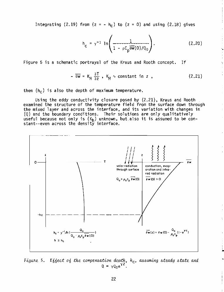
Integrating (2.19) from (z = - hc ) to (z = 0) and using (2.18) gives

(2.20)

Figure 5 is a schematic portrayal of the Kraus and Rooth concept. If

- 8w = KH ~~ , KH ~ constant in z , (2.21)

then (hc ) is also the depth of maximum temperature.

Using the eddy conductivity closure posed by (2.21), Kraus and Roothexamined the structure of the temperature field from the surface down throughthe mixed layer and across the interface, and its variation with changes in(Q) and the boundary conditions. Their solutions are only qualitativelyuseful because not only is (Kh) unknown, but,also it is assumed to be con­stant--even across the density interface.

I I I

f f II I Iz I I I z

I I I0 --- T J J 9w

solar radiation conduction, evap-through surface oration and infra-

red radiation

°0 > Pocp 9wlOl

-hc --------

he = )'-11n I °0 l00 - Pocp 9w(ol

h ~ he

00 yz9wlzl=9wIOl- pc ll-e l

o p

L

FiguJte. 5. E66e.c..t 06 the. c.ompe.Yl.6a.Uon de.tJth, he., M.6wning .6te.adfj .6:tate. a.ndQ = yQoeYz •

22

With regard to the depth of the mixed layer (h), all they could reallysay was it must reach some depth greater than (he)' "Dependent upon theintensity of the convective and wind drive turbulence, this convective regimemay penetrate more or less deeply beyond the level (hc )."

They visualized a steady-state layer depth as being possible only byrequiring upwelling (W>o) of sufficient magnitude to maintain the verticalposition of the entraining interface.

2.6 Prototype Turbulent-Energy-Budget Model: Kraus and Turner

Recognizing the limitations in application of the Kraus and Roothmodel--no provision for a possible downward surface heat flux, no account ofmechanical production of turbulent kinetic energy, and the steady-stateconstraint--Kraus and Turner (1967) further improved and generalized thiskind of one-dimensional model. Their model was the first instance in whichit was recognized that the budgets for thermal and mechanical energies couldbe considered separately. This is valid because the dissipative rate ofheating (PO/J'E) is several orders of magnitude smaller than either Q(z) orIpoC p aew/azl. Therefore, their model consisted of two separate equations-­the heat equation and a mechanical energy equation in which the net effect ofthe work of the wind on the sea surface and the viscous dissipation withinthe mixed layer are parameterized. This use of a mechanical energy equationtogether with the buoyancy (heat) equation and the boundary condition (1.23),

-- () dh- bw -h = ~B dt ' (1. 23)

(2.22)

gave for the first time a clos~d set of equations whose solution providedh(t).

If buoyancy is a function of temperature alone and constant in the mixedlayer, equation (1.25) is applicable. Using the radiation absorption func­tion (2.18) it becomes

d<T> dh Qo -yh--h crt + ~T dt A = -C- (1 - e ) - ew (0) .

Po P

The turbulent kinetic energy equation, integrated from the top of the en­trainment zone (z = - h) to the surface ;s

f aG - D = -89 ew dz

-h

23

(2.23)

-

where 10 aU.

- 1G = - U.W - dz-h 1 az

is the total rate of mechanical production and

D = (0 E:dzJ-h

is the total rate of dissipation within the mixed layer. Neither of theseparameters "in the Kraus-Turner model is an implicit variable, and each mustbe specified externally. The heat equation that leads to (2.22) is also usedto eliminate ew from (2.23) by integrating between z and 0:

(O(d<T> + aew _ JL..-.) dz ~ = a , orJ z dt az~ PoC p

(2.24)

Integrating ew (z) as prescribed by (2.24) from (z = h) to (z = 0) gives

fO _ 1 h2 d<T> [Q~ -aW(Ol]Qo [1 -Yh]ew dz -2 ~-

h +YPoCp

e . (2.25)Po'v p-h

Neglecting e-yh , equations (2.22), (2.23) and (2.25) can be used to giveanother equation (2.26), which together with 1£.22) constitutes a closedsystem in h(t) and <T> (t) where G, D, Qo and ew(O) are prescribed functionsof time at most.

h2 d<T> -Th ~ A = G - D Qo2 ~ + lJ. dt -=-[3-g'::"" + P-

oC-p-y . (2.26)

An important contribution by Kraus and Turner was the conceptualizationof a model for which a stationary or even retreating mixed layer depth ispossible. In such a case where

24

equations (2.22) and (2.26) are still applicable because of the presence ofthe Heaviside unit step function. Setting (h = hr ) in the case of a retreat­ing or steady mixed layer depth, these equations reduce to (2.22a) and(2. 26a).

d<T> Qo -yhrhr (ff""" = PC (l - e ) - ew (0).o p

(2.22a)

(2 .26a)

Neglecting short-wave radiation that escapes the mixed region and eliminating(d<T>/dt) between (2.22a) and (2.26a) gives

h = 2(G - D)r 8g (Q0 - ew (0) )

(2.27}

Whenever the surface boundary conditions and/or solar radiation adjustto make (hr < h) the mixed layer will "retreat. 1I Of course, the region doesnot unmix, in accordance with the second law of thermodynamics. The net rateof production of turbulent kinetic energy, G-D, is insufficient to balancethe rate of increase of potential energy,

al - 89 ew dz,-h

required to mix the region all the way to the density interface. Conse­quently, as the region warms (notice that d<T>/dt can be only positive atthis time), a new density interface is established at z = - hr.

Kraus and Turner model G in terms of the friction velocity:

(2.28)

Not knowing the importance of the viscous rate of dissipation,

25

oD = f E:dz,

-h

they simply neglect it. They find, however, that their model predicts a too­large value for (h), and that the dissipation should possibly be included.

Turner (1969) felt that there was a problem with (2.28) as well. Fromexamination of observations of sudden wind speed increase and ensuing mixedlayer deepening, he deduced that "a substantial fraction of the part of thework done by the wind which goes into the drift current is eventually usedto deepen the surface layer. II This statement reflects the need for a morecomprehensive model, particularly for unsteady situations. Such a modelshould reflect the input of energy into the mean velocity profile and thetime delay needed to shift some of this energy to turbulence.

Again with regard to the Kraus and Turner model, the setting of (D = 0)so that

- 8g

o

~8w dz = G (2.29 )

places an unreal istic constraint upon the buoyancy term: it becomes depen­dent only upon the mechanical production. The error in this is most obviouswhen there is strong surface cooling and

o(- f 8w dz)-h

is less than zero.

Kraus and Turner also neglect the effect of entrainment in their turbu­lent kinetic energy budget, equation (2.23).

In spite of these deficiencies, this model was a big step in the rightdirection in its consideration of the turbulent energy budget in recognitionof the energy source for mixing and entraining.

2.7 Adding Dissipation

Miropol'skiy (1970) and later Denman (1973a) assume that dissipation isa fixed fraction of the shear production, equation (2.30).

D = 0" G

26

(2.30)

where 8~ is an empirical parameter to be determined from observations. Thisgives, instead of (2.29), the equation (2.31):

- 13g Jo

ew dz =

-h(2.31)

This does not solve the dissipation problem because 8~ cannot have a constantvalue. In essence, dissipation must be allowed to adjust to the total situ­ation as it evolves.

Miropol·skiy also assumed that G~ui, but a variation of an exercise heuses to deduce this demonstrates perhaps the major source of error in a model1i ke (2. 28) .

G - - f a (- aU -uw az + vw-h

av) dzaz .

If auw/az = - fV and avw/az = fU, then

[- uw V- uw V]a

G = 'V u3*-h

In general, however,

auw = - fV aU andaz -at ,

av\'J = fU aV givingaz -at ,

f a L (U2 + V2)at 2 dz-h

(2.32)

and thus indicating the importance of the mean kinetic energy and its distri­bution within the mixed layer. As will be shown, even if the wind is steadyfor long periods of time, the mean kinetic energy can change markedly on atime scale corresponding to the inertial period.

Most recently, the trend in the literature has been to model the mixed --layer as a vertically homogeneous moving slab with density and velocitydiscontinuities at the entraining interface. Geisler and Kraus (1969) werethe first to use the slab approach in their model of the atmospheric boundary

27

layer. This problem is almost completely analogous to the oceanic mixedlayer problem except that the atmospheric boundary layer is driven by ahorizontal pressure gradient rather than by a surface stress. A rigid sur­face boundary rather than a free surface also results in a subtle but impor­tant difference. Nevertheless, the basic setups of the two problems are thesame.

Simultaneous calculation of the mean velocity together with (h) and (T)permits the implicit calculation of the mechanical production of turbulentenergy, an improvement upon the previous (u;) method.

The equations (2.33) and (2.34), reflecting the conservations of meanmomentum and mean buoyancy are essentially the same as (1.24) and (1.25).The only real difference is that Geisler and Kraus assume a prescribed meansubsidence (analogous to ocean upwelling) in their atmospheric boundarylayer. This non-zero vertical velocity (W) can result in a stationary mixedlayer depth even when entrainment is occurring. This then is a differentmechanism than that developed by Kraus and Rooth (1961) for obtaining aconstant (h).

r

h d~~> + liC (~~ - W) = - ifh «C> - Cg) - cw (0) •

h dar> + liT (~ - W) = - ew (0) •

(2.33)

(2.34 )

(2.35 )

In (2.33), (- ifC ) is the kinematic geostrophic pressure gradient, thesource of momentum. TRe kinematic surface stress, cw (0) is a momentum sinkin this case.

Geisler and Kraus seem to avoid the problem of dealing with the viscousdissipation of turbulent kinetic energy by prescribing a fixed value for theintegrated flux Richardson number, RfI .

hfa bw dzRf I =j,--;Oh;---.::------~- - n, cons tant .

uw !ll.. + uw ~ dzaz az

This, however, is equivalent to Miropollskiy's method. From (2.31) and(2.35),

n = 1 - o~ . (2.36)

Since (n) is always a fixed positive number, and with no radiationabsorption in the model, the buoyancy flux (heat flux) can only be downward.-rherefore, this model like that of Kitaigorodsky is restricted in applicationto only those cases where the mixed layer is stable throughout.

28

-

2.8 Role of Mean Kinetic Energy

Pollard, Rhines and Thompson (1973) apply the slab approach to theoceanic mixed layer, but they complete the entrainment problem with a differ­ent mechanical energy requirement. The time rate of change of the total meanmechanical energy, potential plus kinetic, of the slab is set equal to therate of work by the wind on the mean flow:

aPE aKE [ - -Jat + at = - U uw - V uwz=O

(2.37)

This is the same as (1.12) integrated from (z = - h - 0) to the surface ifviscous dissipation is neglected and (U) and (V) are constant in (z) withinthe mixed layer. The turbulent buoyancy flux (bw) gives the potentialenergy change using equation (1.11):

aPE _at - -

o

f bw dz = .!. h2 ~ + h ~B ~2 at at .-h

Neglecting the time rate of change of the turbulent kinetic energy,

If radiative heating is ignored, (2.37) reduces to

Ri = h~B = 1 .U2 + V2

Pollard, Rhines and Thompson assume that (2.37) applies as long as

10

• rr (z = 0) • [- U uw - V uw ] 0

(2.37a)

is positive. As soon as this rate of work by the wind becomes negative,"energy flow to increase (h) ceases and since the water cannot unmix, (h)must be constant ... ". Therefore, mixed layer deepening would occur only upuntil one-half of an inertial period following the onset of a steady windstress. This result is demonstrated by setting cw (0) = - u~ and~C = <C> in equation (1.24), giving

d«~~h) + if «C>h) = u~ .

29

-

The particular solution is <U> + i <V> = (iu;/fh)(e- ift -1). Hence ~·U (z= 0) goes to zero when <U> vanishes at time t = w/f.

In this model, energy for entrainment is derived directly from the meanflow. A separate budget for turbulent energy is not considered. That is tosay, the intensity of the turbulence is not considered to have an active role ~

in the mechanism of entrainment in this model.

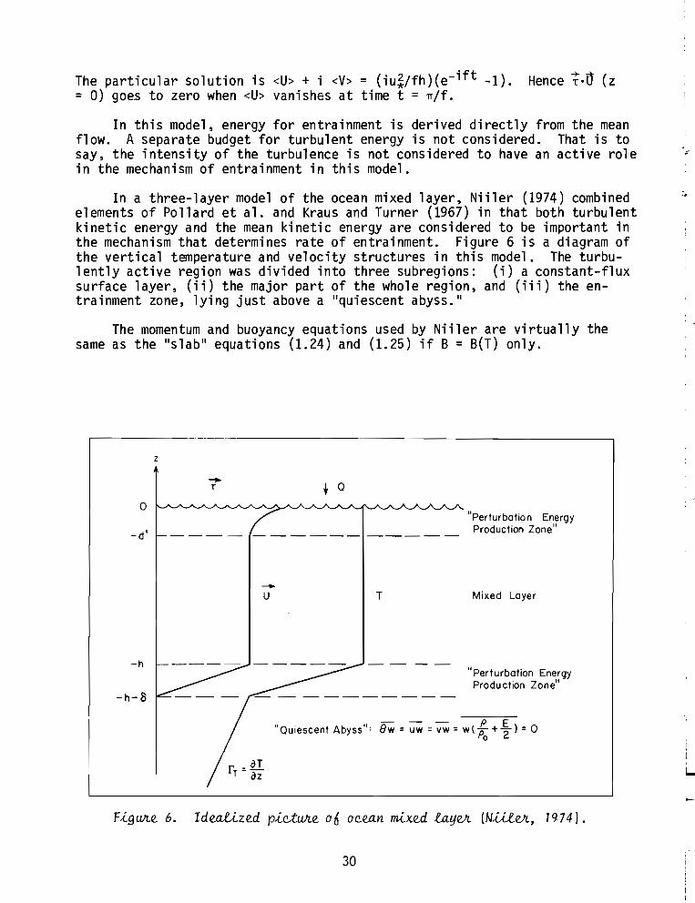
In a three-layer model of the ocean mixed layer, Niiler (1974) combinedelements of Pollard et al. and Kraus and Turner (1967) in that both turbulentkinetic energy and the mean kinetic energy are considered to be important inthe mechanism that determines rate of entrainment. Figure 6 is a diagram ofthe vertical temperature and velocity structures in this model. The turbu­lently active region was divided into three subregions: (i) a constant-fluxsurface layer, (ii) the major part of the whole region, and (iii) the en­trainment zone, lying just above a "qu iescent abyss. II

The momentum and buoyancy equations used by Niiler are virtually thesame as the "s l ab" equations (1.24) and (1.25) if B = B(T) only.

,---------_._---_._-------------------------,

t Q

o

-d'

z

-­T

-u T

"Perturbation EnergyProduction Zone"

Mixed Layer

-h

-h-8

"Perturbation EnergyProduction Zone"

- - - P E"Quiescent Abyss": 8w = uw =vw =w( Po +2") =0

i~

Figwz.e. 6. Ide.aLtze.d pie-twz.e. 06 oc.ean m-Lxe.d la-yell. (N..ulell., 1974).

30

h d<C> + A t:,. C dh = ifh <C> '- cw (0)dt dt

h d~r> = A t:,. T~ = - aw (0).

(2.38 )

(2.39)

Radiation absorption was assumed to occur entirely in the uppermostlayer and was therefore included in aw (0). The additional term (F/po) isa IIdamping li force for inertial motions

(2.40 )

within the mixed layer and presumably is related to the IIldissipation ' ofmean motions as well as the radiation flux of momentum from the bottom of themixed layer. II Pollard and Millard (1970) considered such a term as well, butone that was linear and thus resulting in an exponential damping. The timeconstant (LI) ranged from four to twenty-five inertial periods, dependingupon the size of the inertial circle relative to the horizontal scale of theforcing wind system.

ChpoLI = -F- .

If the mean velocity below the density interface is zero and the meantemperature below the interface is given by T(z < - h) = fTZ, then the fluxesat (z = - h) reduce to

and

-cw (-h) = t:,.C ~~ = <C> ~~

- dh dh- aw (-h) = t:,. T dt = «T> + fTh) dt .

(2.41)

(2.42)

Since T = <T> and C = <C> for the bulk of the mixed layer, the turbulentfluxes are linear functions in (z):

- cw (z) = - cw (0) - f [cw (0) + <C> ~~J . (2.43)

- aw (z) = - aw (0) - f raw (0) + «T> + fTh) ~J. (2.44)

The relative importance of the terms of the turbulent kinetic energy budget(1.13), was hypothesized to vary with subregion.

31I

(1.13)

"II

(2 .45a)o > z > - d"

-h > z > - h - IS

The rate of mechanical production, -uiw aUi/az, was assumed to be non-zeroonly in the surface and entrainment subreglons. In these two regions ofsmall vertical extent, the buoyant damping was considered by Niiler to beinsignificant. Thus the balance is between mechanical production, turbulentand pressure diffusion, and dissipation, equation (2.45a):

;z [w (~ +~ uw ;~ + vw ;~ + < = 0 for

In this model aU/az = aV/az = 0 within the central part of the mixed region,and hence mechanical production is necessarily assumed to be zero. There­fore, here the buoyant damping and viscous dissipation are balanced bydiffusion from the two adjacent production layers, giving equation (2.45b) .

.L [we 2E + L )] - bw + £ = 0 for {- d">z> - h} (2.45b)az Po

Integrating equations (2.45a) and (2.45b) vertically and combining them toeliminate w(E/2 + p/po) at (z - - d") and (z = - h) gives

(- aU - av)uw - + vw - dz -az az

(2.46)+ I <C> J2 dh = _~ dt f

obw dz .

-hIn the manner of Kraus and Turner, Niiler parameterized the sum of the

first three terms of (2.46) in terms of the surface stress.

_ w(L + I) I -Po 2 0 t-d

aU.- 1uiw dZ dz -

of < d z " rna u~ •-d

(2.47) L

32

Integrating (2.42) to give

oj bw dz = - Bg

-h

and using (2.47), equation (2.46) becomes

(2.48)

The system of equations (2.38), (2.39), and (2.48) is a closed set of equa­tions in the three unknowns: - h, <T> and <C>.

This model more resembles that of Kraus and Turner than it does thatof Pollard et al because of the utilization of a parameterized turbulentkinetic energy equation rather than a total mechanical energy equation.The primary difference is the presence of the entrainment production term,I<C>1 2/2·dh/dt, in (2.48) which necessitates the additional equation, theintegrated momentum equation (2.38).

One aspect of important consequence in Niiler1s model manifests the needfor an even more comprehensive term-by-term modeling of the turbulent kineticenergy equation. This is the fact that the turbulent kinetic energy producedby entrainment, I<C>2/2.dh/dt, must go entirely toward increasing the poten­tial energy. Because of the parameterization, (2.47), dissipation is notpermitted to adjust to include either the direct effect of this particularsource, or the less obvious effects related to the entrainment or lack ofit.

The only solution to this predicament would seem to be to model dissi­pation separately from any of the source terms, allowing it to adjust tototal turbulent intensity.

3. CLOSING THE PROBLEM

The equations (1.19a-c), (1.24), and (1.25) do not by themselves consti­tute a closed system of equations for the mixed layer. Vertical integrationover the mixed layer simplified the equations but introduced yet anotherunknown, the mixed layer depth (h).

33

-

3.1 Net Viscous Dissipation in the Mixed Layer

Jo

E dz =

-h-o r-h-o

au. au., ,'J -- dzax. ax.

J J

A dissipation time scale (T E ) is defined by E = <E>/T E •

For fully-turbulent geophysical flows having large Reynolds numbers,viscous dissipation of the turbulence occurs primarily in the small eddiesthat are locally isotropic. As explained by Tennekes and Lumley (1972), aninviscid estimate of dissipation may be made by taking the rate at whichlarge eddies supply energy to small eddies (equal to the rate of dissipation)to be proportional to the reciprocal of the time scale of the large eddies.If the time scale of these large eddies is prgJlg.I:tional to the mixed layerdepth divided by the rms turbulent velocity ~ <t>, then an integral model fordissipation in the mixed layer, independent of viscosity and the small scalesis

oj( £ d z 0 m,<E>'/2 (3.1)

-h-owhere (ml) is a constant of proportionality. For those situations where<E> ~ u~, equation (3.1) is the same as that used by Miropol 'skiy (1970) andDenman l1973).

An important concept in modeling dissipation is that of local isotropy.Turbulent kinetic energy generated at the largest scale (~h) is transferredwithout much additional production or dissipative loss through the inertialsubrange to the larger and larger wave numbers (smaller eddies) by vortexstretching. Dissipation is significant only at the lower end of this iner­ti a1 subrange.

Because there is no preservation of the original orientation, the smalleddies of the inertial subrange are 1I1 ocall y isotropic. 1I Therefore, diss'j­pation draws approximately equally from all three turbulent energy compon­ents. Of course, the existence of an inertial subrange is dependent upon alarge Reynolds number, and this is certainly the case for the oceanic mixedlayer.

3.2 Net Effect of Redistribution of Turbulent Energy

R =II r-h-o

34

iII

L

As previously discussed, R1 + R2 + R3 = 0, but Ra may be an important sourceof sink term for the individual turbulent kinetic energy budgets.

Following the early lead of Rotta (1951), but in agreement with thedominant term of the rational closure technique of Lumley and Khajeh-Nouri(1974) ,

(3.2)

In addition to dimensional consistency, the concept leading to (3.2) is thatof a II return to isotropy.1I In other words, the correlation of pressure andturbulent rate of strain tends to redistribute energy equally among the threecomponents.

3.3 Shear Production

(- aU - av)uw az + vw az dz (3.3)

where loCal is the lIexcessll surface mean velocity in the direction of thewind stress. Notice that in this instance the inhomogeneity of the meanvelocity field cannot be neglected.

JO[!.- w(L + I) J- d z -az Po 2

-h-om" u 3

3 *

where ui = Icw (0) I.If local is proportional to (u*), then (3.3) may be combined with the param­eterized net input from breaking waves less loss to radiating internalwa ves:

G = r-h-o[-aU -aV a (wn WE] 3 Ilic I2 dh- uw - + vw - + - .:.:L + -) dz = m3u +~ - .dZ az dZ Po 2 * 2 dt (3.4 )

This is basically in concurrence with the work of Kraus and Turner, Denman,and Niiler.

35

-

3.4 Need For an Entrainment Equation

Using the suggested relationship (1.24), (1.25), and (3.2), equations(1.14 a-c) become (3.5 a,b). The two horizontal component equations havebeen added together t~ve an equation for horizontal turbulent kineticenergy <q~> = <UT> + <v>, together with the equation for vertical turbulentenergy <w >:

(3. 5a)

(

1 d- - (h<w2»2 dt = ~ [bW (0) - ~B .Q!!. A - ~ Q--] + m2 £ «q2> - 2 <w2»2 dt P oC p

o

where Q' = - J (Q

-h-o

_ .ml _ 3/23 <E> ,

fo

Qdz) dz and <E>= <q2> + <w2> .

Z

(3.5b)

If h (t) is unknown, equations (3.5a,b) together with (1.24) and (1.25)are an incomplete system of four equations in five unknowns: h, <C>, <B>,<q2>. An entrainment hypothesis will provide the fifth equation needed toclose the system.

4. ENTRAINMENT HYPOTHESIS

4.1 Entrainment in Earlier Mixed Layer Models

In this study the entrainment velocity, ue = dh/dt, will be modeledexpl icitly in terms of the other free parameters of the system. However, inmuch of the literature treating models for the ocean mixed layer, (ue) is aconsequence of various assumed constraints placed upon the mechanical energybudget for the layer as a whol~.

In the first really tenable model of the mixed layer that was capable ofsimulating a growing mixed-layer, Kraus and Turner (1967) assumed that allof the turbulent kinetic energy produced in the mixed layer goes to increase --the potential energy of the system. After taking into account any surface

36

buoyancy flux, the balance of the potential energy change went to entrain­ment--mixing the requisite amount of underlying denser water uniformlythroughout the homogeneous mixed region.

Their resultant entrainment velocity is

2 (G - D) + wb(O)h +

(4.1)

where (G-D) is the net rate of mechanical production of turbulent kineticenergy minus the rate of viscous dissipation for the whole layer. Thesurface buoyancy flux wb(O) may either increase or decrease the entrainmentvelocity, depending upon its sign. Again, not knowing how to deal with thedissipation (D), Kraus and Turner ignored it. They set G = ui, so (4.1)becomes

(4.1a)

where the solar heating function (Q~) and the surface buoyancy flux have beencombined in defining a buoyancy flux scale:

(4.2)

Geisler and Kraus (1969), Miropol ·skiy (1970), Denman (1973) and Niiler(1974) all assumed that a fixed fraction of the mechanical production of theturbulent kinetic energy would be di?sipated. Therefore, their resultantentrainment rates are the same as (4.1a) except that some constant smallerthan 2.0 would precede ui.

Pollard, Rhines and Thompson (1973) did not explicitly consider theturbulent part of the mechanical energy budget, and therefore a conceptuallydifferent relationship results from their use of the total mechanical energyequation:

(4.3)

37

If (b* = 0) this reduces to Ri* = 1, or

h >~- liB .

The (~) sign was added to prevent the mixed layer from retreating when meankinetic energy is removed in the second half to the inertial cycle.

This approach at first seems to give a plausible result based upon thestability of the mean flow. The problem is that the mixed layer is alreadyturbulent, and the system has an excess of turbulent kinetic energy, some ofwhich may be available for mixing at the interface, regardless of the valueof the overall Richardson number, Ri*. It is granted that Ri* may be con­strained to having a value greater than some critical value by reason of amean flow instability, but the fact is that in the laboratory and in geophys­ical cases, measurements indicate that entrainment occurs even though Ri* ismuch larger than one.

The entrainment experiments with mean shear of Kato and Phillips (1969)and Moore and Long (1971) (Figs. 7 and 8) show no direct relationship betweenRi* and a maximum layer depth. More importantly, Turner (1968) and othershave conducted experiments with growing mixed layers that had only turbulenceand no mean shear (Ri* = 00).

All of these laboratory results when examined together strongly implythat the bulk Richardson number Ri* is not the parameter most relevant toentrainment rate. Instead, a similar nondimensional number, using the tur­bulent kinetic energy (E) rather than IlICI 2 , is suggested.

As shown by Niiler (1974), the mean kinetic energy can influence entrain­ment rate by increasing (E) in a growing mixed layer. This in turn increasesthe average position of the bottom of an oceanic mixed layer undergoing asequence of entrainment and retreat due to varying wind stress (u~) and heat­ing/cooling (u*b*) cycles. Figure 9 therefore indicates some statistical de­pendence upon the vertically-averaged Richardson number and hence Ri* as well.

4.2 Suggested Turbulent Mechanism

Benjamin (1963) shows that three basic types of instabilities are pos­sible for a system where a flexible solid is coupled with a flowing fluid.At the interface between the mixed layer and the denser water beneath, a so­called class "A" instabil ity will arise if

II ~ 5jf[where (k) is the wave number of the interfacial disturbance,

38

(:

-

1.92 3.84 1.69 ~ X103 cQ•dz

0.995 a • 0

1.485 ~ ~

2.120 0 • +2.150 .. .. •u~ cos

I 10Ri* « (E*r l

100

FigWte. 7. Rate. 00 e.ntJuLi..nme.nt V.6.~Blu~ (Kate and P~p.6, 1969).FigWte. taken oJtom Kantha. (7975).

FigWte. 8. Rate. 0 0 e.~nme.nt V.6.Rlcha.Jtd.6on numbe.Jt, oJtom MooJte.and Long (1971) e.xpe.Jtime.nt.

~ _ eik(x-clt)II - no ,

and (~u) is the total velocity change across the interface.

From Lamb (1932), §232, a class "G" instability, the Kelvin-Helmholtzinstability, requires a higher (~U).

"J "J, !2iB~u >V T-k- .

However, the class "A" instability is dependent upon energy dissipation inthe lower fluid, and this is likely to be small com ared with inferredrates of convergence of energy flux, - alaz [w(p/po + E/2 l-h, at the inter­face. For geophysical flows of this type having large Reynolds and P~clet

39

DEPTH A,ERAGEO RrCHARCSC~ NuMBER. 15.B-26.2 METERS

DEPTH AVERAGED RICHARDSON NUMBER. 26.2-46.2 METERS

4SEPT71

4SEPT7\

30

30

25

25

20

20IS

15

\0

10

100

'".....CDz::

102~II">0

'"a: 1r<.J

c>-

.15

AUG71

100

'"wCDz:

\0::>2

Z0II">0

'"a:r<.J

'".1

5AUG71

FigWLe. 9. Ve.pth-avve.a.ge.d gMdie.nt TUc.haJui.6on numbell, t:.zt:.B/ I t:.C 12 ,

VeJL6U6 time. at :two de.pth JtangM (buoy me.a.6Wl.ement6 C.OuJr;t.My 06Vavid Hai.pelLn) . Vai.uM gfte.a.:telL than 100 Welle. de.6.{.ne.d a6 e.qualto 100. Va6he.d hottizontal -Une. <Lt 1.0 fte.pftMe.YLt6 the. c.ondition60ft ma.Jtginai. dynamic. ~:ta.bilUy.

numbers, the class "G" instability is therefore most likely to be the domin­ant mechanism leading to observed rates of entrainment.

The specific mechanism that is envisioned in the destabilization of theinterface and the resulting entrainment is a "l ocal" Kel vin'-Helmholtz (K-H)instability. The shear needed to trigger such an instability is provided bythe local turbulent eddies. The mean shear contributes to the instabilitybut cannot in itself generate a critical Richardson number. The mean gradi­ent Richardson number

Ri = aB/az(aU/az )2

(4.4)...

would not be likely to achieve a critical value because the total instan­taneous Richardson number,

40

-Ri = ab{az

T (au/az)2(4.5)

is the relevant parameter. The minimum value of the envelope of RiT(t) atthe interface would determine the advent of any appreciable interface insta­bi 1iti es.

The onset of the K-H instability and its exponential growth rate is pre­dicted by linear two-dimensional wave theory. As individual wave packetsachieve a significant amplitude, the nonlinear and three-dimensional effectsof the turbulence field prevail by distorting the wave shapes and advectingparts of the exposed cusps of denser water up into the mixed layer. There­fore, only the initial stages of the instab"il ity are strictly of the K-Htype, where the induced suction at the crests of a perturbation wave on theinterface is large enough to overcome the restoring buoyancy force.

4.3 Relevant Parameters and a Dimension Analysis

Since the mechanical energy needed to continue this mixing process andthus provide for a significant entrainment velocity must come from theturbulent eddies, the rate of supply of turbulent kinetic energy, - a/az[w(p/PQ + E/2)]_h' just above the interface should determine the value of(ue) for a given buoyancy jump (6B) and mean velocity drop 16Cl across theinterface.

As Long (1974) summarizes experimental studies, the nondimensionalentrainment velocity W* is found to depend upon the first power of thedimensionless parameter E* based upon the buoyancy jump across the interface,the depth of the homogeneous layer (h), and the intensity of the turbulence<E>. Where Long assumes <E> a u~,

* <E>E = h6B

* ue *and W = aE.hE>

(4.6)

(4.7)

The relationship (4.7) to~ether with an integrated turbulent kineticenergy equation to provide <E>(t) plus the mean buoyancy equation could beused to close the problem.

The equation (4.7) is appealing because it depends strongly upon thatwhich is accomplishing the erosion of the interfa,e a the turbulent eddieshaving a length scale (~h) and velocity scale (~ <E». However, its usebased only upon laboratory evidence raises some questions about what is

41

really happening in the turbulent kinetic energy budget and why the meanvelocity jump 16CI does not appear to be important at a first glance.

Resorting to a dimensional analysis in which the relevant para~eters are

h, ue ' 6B, 16C/, and <E> gives

where

~ (W*, E*, Ri*) = 0 (4.8)

w* =

<E>E* = h6B

and Ri* = h6B

16CI2

Here, the physical significance of (h) is its assumed proportionality to thelength scale of the turbulent motion respons"ible for the interface instabil­ities.

Re-writing equation (4.8) so as to solve for (ue),

h6B )16CI 2 •

(4 .8a)

The experimental relationship (4.7) suggests that Ri* may be of negli­gible importance compared with E*. Other investigators besides Long, doingdifferent experiments have found varying relationships between w* and E* (SeeKantha, 1975).

The question of why W* would tend to be linearly related to E* in manybut not all cases may be answered by closely examining the turbulent kineticenergy budget in the entrainment zone.

42

,!ii..

4.4 Turbulent Kinetic Energy Budget at the Density Interface andthe Development of a Theoretical Equation for Turbulent

Entrainment in the Presence of Mean Shear

At (z = - h), at the top of the entrainment zone and within the fully­turbulent mixing region, the turbulent kinetic energy equation is

[-aU - av]o = - uw - + vw-az az_h(4.9)

(4.11)

(4.10)tiC Q!!.dt

At (z = - h), the turbulent fluxes are

cw ] -h = -

bw J-h = - AB ¥t- .and

The convergence of flux of turbulent energy at the interface is re­sponsible for the entrainment buoyancy flux, bw(-h).

The problem is to esti~ate the time scale (Te) required to transport some ofthe turbulent energy <E> to the vicinity of the entraining interface.

_~ [W(L + £)J - <E>az Po 2 -h Te

The mixed layer depth (h) or a length scale proportional to (h) is thedistance over which turbulent energy must be transported by the verticalcomponent of turbulent velocity (w). Therefore, (Te) is taken to he pro­portional to (h) divided by the rms vertical velocity scale, I ~2>, givingthe entrainment hypothesis, equation (4.12). This equation is a refinementof what Tennekes (1973) has suggested. The difference is the use ofI <w2> <E> rather than <E>3/2.

43 I

I

a [(L E) ] R><E>az w Po + 2 -h = m4 h . (4.12)

Two possibilities are suggested for how the mean shear at the interfaceshould adjust. The first is according to a gradient-diffusion model havingan eddy viscosity scaling with the integral scales of the mixed-layer turbu­lence. The mean shear becomes

ae _ cwaz = - mshi<W2"">

(4.13)

Then if local dissipation is negligible compared with the flux divergence atthe interface, equation (4.9), using (4.10) - (4.13), becomes

= 0 • (4.14)

For those cases where <WZ> is proportional to <E>, (4.14) can be reduced tosimply

*(w )2*Ri

m§

* m4 * *(w ) + -- E Ri = 0

m§(4.15)

in non-dimensional form. Solving (4.15) for W* gives

*W* = B..:!..- -

2m§

m4 * *- -- E Ri

m§or

where

* Ri * [ ]W - - 1 - 11-4</>*2m§

44

(4.16 )

(4.17)

,!,

If ~* < ~, the binomial expansion gives

11 - 4 ~* = 1 - 2 ~* - 2 ~*2 -4 ~*3 - . . . .

and therefore (4.16) may also be written as

w* = m4 E* (1 + ~* + 2 ~*2 + •••• ) • (4.16a)

For small ~*, (4.16a) rapidly converges and onl~the first term may beneeded. For more general applications, where <w > is not always proportionalto <E>, the equivalent solution to (4.14) is

dh m4~ <E>at = hl1B (4.18)

A second possible way for the mean shear at the interface to adjust isso as to maintain a gradient Richardson number of critical size, Rio. Thenin place of (4.13), the thickness of the interface (0) adjusts so that

where R" MB'o=wrz·

(4.19)

(4.20)

In this case, equation (4.9) becomes

45

(4.21)

ordh _dt -

m~ ~ <E>h~B

(4 .21a)

If Ri Q is a constant of order one, then (4.20) predicts, independent of theentralnment equation (4.21a),

o 1-h "'~

Ri(4.22)

4.5 Comparison with Moore and Long (1971) Experiment

Figure 10 is a fit equation (4.16) to the results of Moore and Long(1971). The constants (m4) and (m§) are determined by the best fit. Noticethat in this experiment (E*)-l happens to be proportional to Ri*. This isprobably due to the experimental method and has no general significance forthe ocean mixed layer. Also, w* can be interpreted only as a dimensionlessentrainment flux for this experiment because the experiment involves twoturbulent mixed layers, each entraining the other equally, resulting in amotionless interface, giving

I,

10 1

1/(39.4E*)

~

10-5b.......,- .w.1-J....l11_---'-1---,--I--'-'-..LLl-.W-_-'--.I.....-'--'-'-.............

10°

46

F,[gU!1.e 10. Theonilic.af. en:tJtain­ment c.wwe v.o. da.:ta. 06 Mooneand Long (1971). An ,[n.o:ta.bilily,[.0 pnedic;ted at E* =0• 036. The.oiope appnoac.he.o (-1) a..o E* de­c.Jtea..o e.o •

,....

-bw( -h) = -uw( -h)w* =

flB I:E> flU I:E>

The lowest order term of (4.18) agrees with the general theory of Krausand Turner (1967) and the experiment of Kato and Phillips (1969) for thoseinstances where

The higher order terms of (4.18) contribute to the entrainment processby a feedback mechanism that seems to explain the large-scale instabilityobserved by Moore and Long for small Ri*. Equation (4.18) predicts aninstability when Ri* s (Ri*)cr

where (4.23)

For the Moore-Long experiment, (E*/Ri*)cr = 0.105, or

(Ri*)cr = 9.55 h~~ . (4. 23a)

Although this instability seems to be possible in the laboratory, it is notclear whether it can ever occur in the oceanic mixed layer because the ex­pected turbulent entrainment attributable to the turbulent flux convergence(4.12) alone is sufficient to increase (hflB) at a more rapid rate than Ri*may decrease.

The instability observed tends to verify the gradient-diffusion hypo­thesis, equation (4.13), at least for small Ri*. However, the constant -Riohypothesis, equation (4.19) seems to be a better fit for aU/az(-h) over mostof the range of E*. Figure 11 is a plot of the observed (o/h) versus thevalues predicted by equation (4.22).

Of course, the side walls in flume experiments of this type prohibitpushing the results too hard, but it is fairly clear that the Moore and Longexperiment as well as the others mentioned verify the lowest order term of(4.18a) as well as (4.21a)--no matter how aC/az(-h) is modeled. Thereforethis shall be taken as the entrainment equation:

47

-

F.{.gUIle. 11. PILe.cUete.d -i.nte.Jr.6ac.e.~lope. and MooILe. and Long me.~­

UIle.me.nt6 Ve.MU6 cUme.~-i.onle.M

bUD yanc.y 6lux..

o 0.8 1.0 1.2 1.4

bw 3t.Bt.U xlO

(4.24) ;c

4.6 Completed Model for Shallow Mixed Layers

Equations (1.24), (1.25), (3.5a,b ) and (4.24) constitute a closed setof five equations in the five mixed-layer variables:

h d~i> = - 8C ~~ A - if <C>h - cw(O) (1.24 )

of Qdz - bw(O)

-h-o(1.25 )

1 d 18CI2 dh ~ 2ml - 3/22 dt (h <QT» = m3 u3 +~ dt A - m2 / <E> «QT> - 2<W7» - --3-- <E> •

(3. 5a)

1 d ~- - (h <w»2 dth dh ml - 3/2

= - ~u*b* + 88 CIt A) + m2 I<E> «QT> - 2 <W7> ) - "3 <E> .

(3.5b)

dh _ m,+~ <E>Of - h88

48

(4.24)

I...

In addition to Q (z,t), other specified (external) conditions are the surfacefluxes u*b* and cw(O).

Starting with initial conditions on <C>, <B>, <qL>, <WL>, and h, themodel is solved as an initial-value problem in time.

Also to be specified separately are the initial profiles of Band Cbelow the bottom of the mixed layer. These two variables contribute to ~C

and ~B, which are important for a deepening mixed layer:

~B = <B> B (-h -0)

~C = <C> - C (-h -0)

5. BEHAVIOR OF THE EQUATIONS

5.1 Nondimensional Form of the Turbulent Energyand Entrainment Equations

(4.25)

(4.26)

Using the surface flux scales u* and b*, new dimensionless variables aredefined:

* u*b* hH = (5.1 )

2m3 u*3

p* = h~B dh . (5.2)2m3u*3 dt '

2/3ml <E> (5.3)E* .. = (-)

" m3u~

m1 2/ 3<WL> (5.4 )E*33 = (-)

m3u~

H* is the ratio of buoyant damping (production) from surface heating (cool­ing) to wind-stress production. p* is the ratio of energy lost by entrain­ment (potential energy increase) to wind-stress production.

Invoking the quasi-steady state assumption for the turbulent energybudget, the entrainment and turbulent energy equations become

49

PIp* = "2 E*i i IE* 33 ,

O = 1 + p* (E* 3E) ~* - £ (E* )3/2Ri* - P2 ii - 33 l't.~ii 3 ii '

(5.5)

(5.6)

and

where

o = - H* ~ p* + 02 (E*ii - 3E*33) IE*ii - ~ (E*ii) 3/2 , (5.7)

m4 m2PI - ITi1 and P2 - ITi1 . (5.8) , (5.9 )

5.2 Determination of the Constants

The ratio m2/mi = P2 is equivalent to (18 lI/A) where (lI/A) is theredistribution to dissipation length scale ratio of Mellor and Herring(1973). From boundary layer data, they suggest

11~ = 0.05 ± 0.01 .

Hence P2 is of order one and will be taken to be equal to one in this anal­ysis

1811P2 = -A- '" 1 . (5.10)

The ratio m4/mi = PI may be determined from the asymptotic case of pureconvection, H* + - ~ and Ri* =~. The equations yield

2

I'E* /E* ..33 11(5.11)

whereE* 33 _ 1---(1+ 2 )E* .. 3 ~

11for large Ri*. (5.12)

The fraction (r) of turbulent energy converted to potential energy by entrain­ment is found to be 0.036 ± 0.031 by Farmer (1975) from measurements underthe ice. Using P2 = 1 and r = 0.036, equation (5.11) gives (PI = 0.1).

50

p* may now be solved as a function of H* and Ri*. Figure 12 shows p*(H*) for Ri* = ~ and Ri* = 1.

The one remaining constant needed to complete the model is m3. This maybe determined from the Kato and Phillips results, Figure 7, together withP*(H* = 0) from Figure 12.

This gives m3 = 55.

P*(o) = h~B dh (b = 0) = 0 0227dt * ..21ll3 U*3

(5.13)

(5.14)

However, this value seems to be quite high for an oceanic mixed layer.The conceptual model for the mixed layer developed earlier, equation (3.3),implies that

-0.8

,, 0.06,

Ri* c' ,j', 0.05

r " p*~*=oo , Q~

'\,,~.03

0.01

-0.2H*

o

51

FigWte. 12. Model. .6olut<-on nOlL.6 ha.il.ow rn.ixe.d lalje.Jt.6: po:te.ntia.le.ne.Jtg Ij Jta.:te. a n ,[nCJte.a..6 e. due. :toe.n:tJta.,[nme.n:t Ve.Jt.6 U.6 lalje.Jt .6:tabil­lilj •

where oC o is the excess surface and wind-drive current:

oC o = C (Z = 0) - <C> .

A more moderate value of m3 ~ 10 is expected. In the laboratory experiment,the production was enhanced by the side-wall boundary layers, resulting in atoo-large value for m3.

There is another method of determining (m3) which is suggested by Fig­ure 12. Rather than using neutral (H* = 0) stability situations (stormsituations are only approximately neutral by virtue of a large u*3 comparedwith u*b*h ), cases of limiting strong stability where p* = a and h = hrcould be examined.

H*max = 0.4 = u*b*h so,2m3u* 3

m3 = u*b*h (5.15)0.8 u* 3

The effective buoyancy flux u*b*, given by equation (4.2) should properly bedetermined by measuring Q(Z), and the mixed layer depth h = hr should beascertained to be in the "retreat mode": dh/dt:s O. This method remains tobe attempted.

5.3 Comparison With Earlier Models

The dotted straight line in Figure 12 is equivalent to the solution forp* (H*) if equation (4.1a) is calibrated to behave properly for both the re­treating (H* = H*max) and neutral (H* = 0) situations. The greatest differ­ence between the two models then occurs as H* becomes increasingly negative.This inability to calibrate the earlier model to both stable summer andconvective fall situations has been demonstrated by Thompson (1974).

Nearly equivalent to the Kraus-Turner type model for entrainment,equation (4.1a), is Tennekes's model which suggests in effect that

p"p* = --2

1(E* .. )3/2

11

52

(5.16)I..

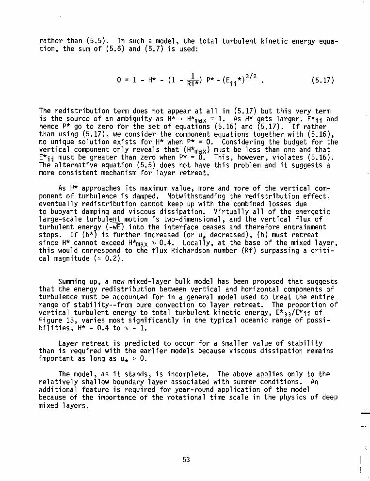
rather than (5.5). In such a model, the total turbulent kinetic energy equa­tion, the sum of (5.6) and (5.7) is used:

0= 1 - H* - (1 _ ~*) P*_(E .. *)3/2R, " • (5.17)

The redistribution term does not appear at all in (5.17) but this very termis the source of an ambiguity as H* + H*max = 1. As H* gets larger, E*ii andhence p* go to zero for the set of equations (5.16) and (5.17). If ratherthan using (5.17), we consider the component equations together with (5.16),no unique solution exists for H* when p* = O. Considering the budget for thevertical component only reveals that (H*max) must be less than one and thatE*ii must be greater than zero when p* = O. This, however, violates (5.16).The alternative equation (5.5) does not have this problem and it suggests amore consistent mechanism for layer retreat.

As H* approaches its maximum value, more and more of the vertical com­ponent of turbulence is damped. Notwithstanding the redistribution effect,eventually redistribution cannot keep up with the combined losses dueto buoyant damping and viscous dissipation. Virtually all of the energeticlarge-scale turbulent motion is two-dimensional, and the vertical flux ofturbulent ener9Y (-wE) into the interface ceases and therefore entrainmentstops. If (b*) is further increased (or u* decreased), (h) must retreatsince H* cannot exceed H*max ~ 0.4. Locally, at the base of the mixed layer,this would correspond to the flux Richardson number (Rf) surpassing a criti­cal magnitude (~ 0.2).

Summing up, a new mixed-layer bulk model has been proposed that suggeststhat the energy redistr"ibution between vertical and horizontal components ofturbulence must be accounted for in a general model used to treat the entirerange of stability--from pure convection to layer retreat. The proportion ofvertical turbulent energy to total turbulent kinetic energy, E*33/E*ii ofFigure 13, varies most significantlY in the typical oceanic range of possi­bilities, H* = 0.4 to ~ - 1.

Layer retreat is predicted to occur for a smaller value of stabilitythan is required with the earlier models because viscous dissipation remainsimportant as long as u* > O.

The model, as it stands, is incomplete. The above applies only to therelatively shallow boundary layer associated with summer conditions. Anadditional feature is required for year-round application of the modelbecause of the importance of the rotational time scale in the physics of deepmixed layers.

53

-5

E*lim ~= 5/9

h'-CD E~

0.5

0.4

FiguJte 13. Rmo on veJt.ilc.a1. -tuJtbui.entfUne;Uc. eneJtgy -to -to-tal -tuJtbutentfUne;Uc. eJ1eJtgy a!.l a. nunction.

o 0.4H*

6. DEEP MIXED LAYERS: LIMIT TO MAXIMUM DEPTH

6.1 Limiting Dissipation Time Scale

The need for a constraint upon the maximum depth of the mixed layer hasbeen demonstrated. Niiler has pointed out that models of the Kraus-Turnertype will continue to deepen incessantly during each winter cooling period.This is the unavoidable consequence of requiring some fraction of the netproduction of turbulent energy to be allotted to increasing the potentialenergy by means of entrainment.

Thompson (1974) also found this to be true. In doing a year-roundintegration, the model required an unrealistic value for mean annual surfaceheat flux yielding a net heat storage in order to achieve a realistic cycle.

Outside of the tropical latitudes and away from the continental shelves,lateral advection and upwelling are insufficient to balance this heat stor­age. The most noticeable failure of the model is at mid-latitude regionshaving a permanent pycnocline.

The model for dissipation is still

<I>E 'V ­

TE

However, the dissipation time scale (T E) was previously (in equation 3.1)governed by the depth of the mixed layer and the turbulent velocity scale,giving a strictly convective time scale:

TE

0: -- 'V

54

h

II>

As planetary rotation begins to rotate the mean shear profile, and hencethe geometrical aspects of the integral scale, there arises a new lengthscale, associated with the coriolis time scale (f- 1 ).

Q,2 = I:E> f .

It is now increasingly clear from such studies as those by Arya andWyngaard (1975) and Sundararajan (1975) that the coriolis time scale (f-l)plays an important role in the internal structure of the convective planetaryboundary layer or mixed layer. The concern here is more with the bulk pro­perties of the region and less with the details within the mixed layer.However, it is suggested that this time scale has an important role in theoverall turbulent energy budget above and beyond the turning and decay withdepth of the mean velocity in the classic Ekman spiral. In reality the twoeffects are inseparable because of the link through local shear production.

Rather than to simply replace the convective scale (Q,l) by the rota­tional scale (Q,2), the suggestion is to use Q,-l = Q,i 1 + Q,i 1, giving equation(6.1),

(6.1)

Replacing (3.3) in the bulk (vertically integrated) formulation is equation(6.2)

(6.2)

where

(6.3)

and, as before,

* = (~) 2/3 <E>E •." m3 u 2

*

55

6.2 Nondimensional Solution to the Entrainment Function

Equations (5.6) and (5.7) will now change to reflect the new term, giv­ing (6.4) and (6.5).

p* 2 ~o = 1 + Ri* - P2 ( E*ii - 3 E* 33) IE*i i - 3" E*i i (/E*i i + Ro -1 ) • ( 6•4)

o = - H* - p* + P2 (E* .. - 3 E*33)~ - ~ E* .. (~+ R~-I). (6.5)" " ,)" "

The entrainment equation, (5.5), remains unchanged.

PIp* = -2 E* .. IE*33 •

"*The solution to P is now a function of two variables, and is shown in

p* = p* (H*, RO-I)

(Figure 14).

(5.5)

Specifically, several aspects concerning this nondimensional solutionshould be observed:

a. The solution for Ro- I = 0 is identical with the earlier solution(Figure 12). This limit applies to both the case of shallow (h«u*/f) mixedlayer and the case of very low latitude, cf> « u*/lnlh.

b. For a retreating (p* = 0) mixed layer, hr is now a function of boththe Rossby number and the stability H*. Actually, hr is uniquely determinedby the product of these two parameters, making it a function of

A fairly good analytical approximation to this function is the hyperbolicrelationship (6.6):

56

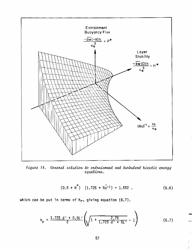
EntrainmentBuoyancy Flux

-bW(-h)h = p*

u;Layer

Stability

-bW(O)h=H*u 3*

F-i..guJLe. 14. Ge.neJr..a.l..6 o.t!.Luon to e.ntJuUnme.nt and tuJLbu£.e.nt fUnetic. e.neJl.g ife.qu.a.tiOn.6 •

* "(0.5 + H) (1.725 + RO-l) = 1.552 .

which can be put in terms of hrt giving equation (6.7).

1+ 2.76 1)1.725 d" + 5L" -

57

(6.6)

(6.7)

where d~'is proportional to the Ekman depth of frictional resistance and L~

is proportional to the Obukhov length scale.

The approximate solution for retreat, equation (6.7), has limitingcases of d~ + 00 and L~ + 00 that are in agreement with the earlier works ofKitaigorodsky (1960) and Rossby and Montgomery (1935).

(6.8)

(6.9)

Physically, the reason for the cessation of entrainment is ultimatelythe same for the convective boundary layer whether or not there is signifi­cant surface buoyancy flux. Dissipation that is approximately equa!!x divid­ed among the three components of the turbulent kinetic energy (UT + v2 + WT)causes <WT>to be consumed more rapidly than it can be replaced by the pres­sure redistribution or "return to isotropy" effect. When this happens, thevertical flux of all properties, including the turbulence itself, ceases atthe depth h = hr. Buoyant damping or production modifies the overall budget,changing the relative value of hrf/u*, but dissipation plays the ultimaterole.

Buoyant production may be sufficiently strong (H* < -0.5) that dis­s~ation cannot limit maximum mixed layer depth. Then the production of<w > is too great to be overcome by dissipation with increasing depth.

c. A cyclical steady state is now possible. The surface buoyancy fluxmay go through an annual cycle having no net heat storage and (h) will notincrease without bounds at the end of the cooling phase.

The simplest steady state is the neutral stability point represented bythe coordinates (R6- 1 , H*, p*) = (1.38,0.,0.). This is the situation for aneutral boundary layer, (bw(O) = 0), where hr = 1.38 d~.

A simple cycle having a sinusoidal variation in bw(O) and a constant u*is qualitatively depicted by Figure 15. This depicts the locus of coordin­ates for (Ro-l, H*) as the cycle progresses through a heating (bw(O) < 0)and then a cooling (bw(O) > 0) phase. The initial [0] and [4] points coin­cide at the neutral steady-state point. Between [0] and [1] buoyancy flux isdirected downwards and is increasing, and the mixed layer retreats to itsminimum depth which occurs at [1]. Between [1] and [2] there is activeentrainment but the rate of entrainment is slow because of significant buoy­ant damping in the stable mixed layer. This would correspond to the summerwarming period, culminating in maximum surface temperatures at about [2].Cooling begins at [2] and reaches a maximum at [3]. Not until the end of theperiod does the rate of entrainment become significant because the heatingperiod [0]- [2] causes a potential energy deficit in the system which must bereplaced before deep-ending may proceed rapidly. In the time period just

58

I,l

- bw(O)IIIIII I

h ,I I

II

I I0 2 4

H* ex -bw(O)hU3*

(0,0) (0,04)

/'/'

//

//

2 /=----l-/-/* I

/

~//

//04--_ ... '

( 1.38,0)//

//

//

//

/

3~*(

Ei.guJl.e. 15. CycUc.a1. -6:te.ady -6:ta:te. -<.n :the. (H*, Ro - 1) plane..

59

I'

after [3] erosion of the thennocl ine is enhanced by both increased systempotential energy and by buoyant production which remains strong even though(bw) is decreasing.

Of course, the real oceanic system is not in an exactly repeating annualcycle. However, year-to-year variations resulting in long-term changes inheat storage can be predicted accurately only by a model that can simulatethe hypothetical cyclical steady-state. Any net annual buoyancy flux acrossthe surface that is balanced by advection is not of concern in studying themod~ in the one-dimensional form. In any case, a large seasonal variationin bW(O)--and u*2--and the resultant cyclical response are dependent upon theproper model response for the more simple situation.

6.3 Simple Hypothetical Cases Demonstrating theBehavior of the Solution

6.3.1 Shallow or f ~ a (Ro » 1).

(1) Initial linear stratification

(a) bw = 0, u; = constant

The result is the same as that predicted by the Kraus-Turner type modelas well as by the Kato and Phillips experiment. See Figures 16 and 17.

dh u 3dt a: K!B

giving

The reason these models are in agreement is that with b* = 0, u* is the onlyturbulent velocity scale.

(b) Free convection: bw(O) = constant> 0, u; = O.

This situation is out of range for Figure 13 because H* + - 00. How­ever, if the model equations are nondimensionalized on the buoyancy fluxvelocity scale (u*b h)1/3, rather than on (u*), the problem may be solved.In this case, h a: tY/2, which is also in agreement with the Kraus-Turner typemodels.

60

1

i

I..

0

-4.00

Ul -8.00 -~

hQ) ..-Q)-12.00~

-16.00

20.00

19.90u01 19.80 -

<T>Q)

019.70

19.60

In0.800 ! I I I I

'0 t-- -t--

x OAOO t-- -..... r- -'0

0$E r-- -0 -0.400 I- - [ew]O --

u -

01 -0.800 -I I I

-Q)

0

0.25 I I I

0.20C\l

0.15• -0Q)Ul

C\l 0.10 fo-

u2E0 it-

0.05 C-

OoI I I I I

20 40 60 80 100 120Hours -Ei.gWLe. 16. Solution :to h(:t) nO!l. C.Me. w.U.h bu;ti.ai. Li.ne.aJl ~t:Jta.:UM-c.a.:ti.on;

ow(O)=O,u~ = c.o~:tant.

61

-5

-10-

-15-

-10 -

-15 -

Figwr.e. 17. Te.mpeJuLtwr.e. pllO 6ile. at 12­howr. -inte.Jtva.i!.l 60ll Mve. dalJf." f.,:taJLt­-ing wUh an -irUtiaf. line-all f.,:tJr.a;UM­c.a:ti.on. The.Jte.,{.f.; no f.,wr.6ac.e. he.at6.tux and a C.OMtant wind f.,:tJr.e.f.;f., ,{.f.;hnpOf., e.d at .tUne. ze.Jto.

- 30 _... L. ...__ L - . ..L .. _ -1 .. -'---_---'18 19 20 21

Dog C

(c) Cyclical surface buoyancy flux: bw{O) ~ sin wt, u~ =constant.

Figures 18 and 19 show the response of the mixed layer to a simplehypothetical diurnal heating and cooling cycle. The magnitude of the heatflux was chosen to be particularly large in order to accentuate the featuresin a relatively short time span. The initial stratification is the same asfor the earlier neutral (bw{O) = O)run, 1°C/20m. The wind stress is also thesame, 0.2 dynes.

Over the five-day period there is an overall cooling trend because ofthe entrainment process and lack of net surface heat flux. However, thedaily maximum surface temperature is greater than the initial surface tem­perature for all five days.

Starting with the fourth day, there is larger retreat corresponding tothe decrease in the Obukhov length scale relative to the value of h. Inspite of midday retreat, the mixed layer more than recovers the temporarilydecreased vertical extent. Without eventual enhancement of dissipation,deepening would continue without bound.

A comparison between Figures 18 and 16 demonstrates another importantdifference, in addition to the presence of a strong diurnal layer temperaturechange. Although there is no net surface buoyancy flux for either case, thesituation having the diurnal cycle has a distinctly slower average rate ofdeepening. This holds even for the first three days when there is no re­treat.

The explanation for this phenomenon lies in the nonlinearity of p* (H*)(Fi gure 12).

62

<T>

I

-

-2

U* -

-I

120 140I

I

100

I

I

80I

I

6040

I

I20

I

I

0

III -4.00....Q.l h....Q.l -8.00~

-12.00

20,80

u 20.400'Q.l0 20.00

19.60N

'0 2.000x

1.0001(,)

Q.l 0III

E(,) -1.000u0' -2.000Q.l0

0.25

0,20N1(,) 0.15 I-

Q.lIII

N 0.10 f0-

E(,) 0.05 I--

00

Hours

F-Lgwr.e. 18. Solution to h (t) 60ft C.Me. will c.1jc.Uc.al .6wr.6ac.e.heat 6fux.; ew (0) = O. 015 .6-Ln (Wi:). CompMe. wLth F-Lgwr.e. 16.

(d) General: U*2; 0, bw(O) ; 0

Since the earlier model projects a linear P*(H*), only two points (attwo values of H*) may be made to a~ee with this model. For example, ifsummer "retreat" and the neutral (ow(O) = 0) cases are coincident in bothmodels, then the winter deepening rate will be greater for the earliermodel. This is the mathematical difference in the basic responses.

63

- 5 -

-10

'"I -15 r-10

-15 -

F,[gWle. 19. Te.mpe.JtatuJl.e. p!l.O 6ile. 60!l.C.Me. wah '[rU-Uai.. Une.aJL -6tJr..ah..M­c.ah..on, wUh c.tjc.Ucal -6Wl6ac.e. he.at6lux. Compa!l.e. wUh F,[gWle. 17.

111019-30 L-_~_--.L-_--L_----'-_----'_----'

18

Dog C

The physical difference may best be seen from the Tennekes (1973) modelin which

]- 3/2

- <E>-bw a: h-h

and

-E 3/2 3 b h< > a: m u* - u* * .

This model is identical in response to the Kraus-Turner model and is suitabJefor comparison here because it identifies the turbulent velocity scale 1<[;.Then retreat (dh/dt < 0) can occur only when <E> + OJ

Tennekes did not intend for this fornlula to be extrapolated to thestrongly stable situation. Instead, he suggested it as an interpolationbetween the neutral and free convection cases--the typical atmosphericboundary layer range. Nevertheless, the above is equivalent to recentoceanic applications of the Kraus-Turner type model. The particular problemwith applying this method to the stable, retreating mixed layer is that theremust still be significant turbulent energy «E> > 0) above z = - hr. Conse­quently, the fraction of turbulent energy going to increase the potentialenergy cannot be independent of stability, H*. This explains the curvatureof P*(H*) and the slower rate of damping for the hypothetical case with anosci 11 ating surface buoyancy fl ux.

64

(2) Cyclical surface buoyancy flux

No 1-D steady state is achievable because for f = 0, h can be limitedonly by the Obukhov length scale, therefore requiring a net downward .buoyancy flux (or heating). Then bw{O) could be balanced only by advection.Gill and Niiler (1973) have shown that advection is insufficient for lati­tudes greater than about 15°.

6.3.2 Convective planetary boundary layer with order one Rossby number

(I) Neutral steady state

With zero surface heat flux, a steady state is predicted (see Fig. 14 atthe limit h + 1.38 u*/f). Starting from an initial linear stratification andh < u*/f, steady state would be approached only after a relatively long time.This is not likely to be achieved in geophysical flows, except perhaps by theatmospheric boundary layer during the polar winter. See Businger and Arya(1974).

(2) Cyclical steady state

This situation has already been qualitatively described and illustratedby Figure 15, but the relative importance of the rotational and surfacebuoyancy flux scales needs to be estimated.

For the sake of studying the relative response of the mixed layer, allcycles will be assumed to be repetitive (in steady state). A sinusoidalsurface buoyancy flux and a constant wind stress are used to drive themodel.

T =

bw{O) = - Ibw{O) I sin wt .

The layer response is found to be a function of the parameter B*, theratio of the buoyancy flux scale to the rotational scale. <

B* = IbW{O) I .f u*2

(6.10)

Figure 20 shows the cycle of h(t), nondimensionalized on u*/f as a functionof B*.

For large B*, which is typical of the annual cycle for temperate oceanicregions, the low minimum mixed layer depth at wt = ~/2 is attributable to thestrong influence of the buoyant damping corresponding to a small positiveObukhov length scale.

65

Phase (wI)0°,-- ----T-7T ..;27T::.-.,

..::J'-::=:; 0.5a.Q)

aQ;>-.3"0c:o

"Vic:

E 1.0'0c:oZ

B*= 10

FigMe. 20• CycUc.a.f.. J.d.eady-J.,t.o.:te.mi.-xe.d-layelL Jl.e6 pon6 e. to .6..tnu­.6o..tda£. .6M6ac.e. buoyanc.y 6fuxand C.On6ta.n.t w..tnd .6:tJr.e6.6.T=pou*2; ow(O)=-low(O) 1.6..tn{wt).

1.5 '-- ----'- ----"OL.--L----J

In addition to the change in the range of h with B*, there is animportant change in the shape of the function h(t). For the case of weakheating and cooling, the variation in h is almost in phase with bw(O). Inthe H* - RO-l plane (Fig. 21), the locus of the cycle would be small andelongated. For increasingly larger B*, the heat and therefore buoyancy isstored during the "summer" at an increasingly shallower depth (in comparisonwith hmax ~ u*/f). This creates a substantial potential energy deficit which

H*

Ro'-I

/'/'

/'/

//

//

//

//

/I

/

If'!/

//

//

//

//

66

F..tgMe. 21. CycUc.a£. .6:teadY-.6:ta:te...tn :the. (H*,Ro-l) plane. 6oJl. ve.Jl.If.6ma.ll c.ycUc.a.l .6M6ac.e. buoyanc.y6fux (8*« 1) •

results in a hysteresis effect by retarding ,the entrainment process. Thisphase lag in the heat storage naturally has important implications for theinteraction with the atmosphere for all cyclical time scales--from one day toperiods of climatological importance.

(3) Fluctuations in wind stress: storms

Fluctuations in the wind stress, particularly in the instance of storms,are very important in the annual evolution of the mixed layer and the heatstorage of the upper ocean.

Running the model for a simulated annual heating/cooling cycle asbefore, but adding periodic "storm" pulses of wind stress gives qualitativelylittle apparent change in h{t). (see Fig. 22). However, the spikes in theretreat side caused by the storms greatly enhance the storage of heat atdepth. The midsummer profile (Fig. 23) with the step-like remnants ofearlier storms, has an overall potential energy significantly greater thanwould be the case with no storms. This, in turn, will tend to enhance theeventual deepening, countering to some degree the hysteresis of the heatstorage in the annual cycle. The annual range of surface temperatures (seeFig. 24) is less than it would be without storms because of the increasedheat storage at depth.

F.£gwr.e. 22. Mixe.d la.yeJr.. de.pth h (t lnOll. hypothetic.at a.nnual C.lfde..£nducUng I.>:toJUnI.>: CMe. A; modelw.U:hout cUwr.nat c.yde..

-100 L-----'--------L...l..._-'-----'-------.l..._-'-----'-------.l..._-'----J

5 7 9 13 15 17 19 21 23 25Deg C

F.£gwr.e. 23. Midi.> ummeJr.. tempeJr..Mwr.e. pll.O­nile. nOll. C.Me. A, model. withoutcUwr.nai. c.yde.•

0

-10

-20

-30

Vl -40...Q)

Qj -50~

-60

-70

-80

-90

-80

-90 -

-100 0'--L....II..-----L-L..-....L--7r...L..---L------l.-...L..--...LJ....---,-J27r

Phose of Annual Cycle

...Ql

i;' -60...J"0~ -10~

-10

-20 ­~~ -30E.r: -40a.~ -50

67

6.4 Filtering Effect of the Storage of Turbulent Kinetic Energy

The hypothetical solutions shown in Figure 20 are all for periods(2n/w) much longer then the integral time scale of the turbulence~ governedby the dissipation time scale (T E). This made possible the assumption ofquasi-steady state so that the turbulent energy storage terms~ a/at <uiui>~

could be neglected in the solutions. However~ fluctuations in the surfaceboundary conditions U*2 and bw(O) of sufficiently short period require theconsideration of these terms.

A very simple model~ which may be solved analytically~ provides theanswers to the question concerning the importance of this unsteadiness andhow it might be treated.

In the simple model only the two largest terms~ shear production anddissipation~ are balanced by the time rate of change of the turbulent kineticenergy.

- - u3

a~i> + ~E> = h* (l + a sin wt)E

(6.11)

The prescribed shear production is a constant plus a sinusoidally-varyingcomponent (a < 1). By defining dimensionless time~

T* = tiT E ~

25 ,-----r---r-.,------,-----r-...,..-----,--,,----,----,

23

21

19

17

(6.12)

u:? 15o

13

II

9

7

7T

Phose of Annual Cycle

Figwz.e. Z4. Swz.na.e.e. tempeJLatwz.e.T(Z=O,tJ non the. hypothetie.at e.a.6e.w.Lth .6toJUn.6: Ca.6e. A, model. wU:houtcUwz.nat e.yc1..e..

68

and turbulent energy,

(6.11) is transformed to (6.14),

h<E>'1'* - --u3 T* E:

(6.13)

where

a'1'*~ + '1'* = 1 + a sin W*T*,

W* = T w.E:

(6.14)

(6.15)

For (a = 0) the steady-state solution is simply '1'* = 1. For finite (a), thecomplete solution, neglecting the initial transient, is

'1'* = 1 +( a ~ (sin W*T* - w* cos W*T*) •w*2 + 1) (6.16)

There is a phase shift that increases with (w*), but the important aspect of(6.16) is the relative magnitude of the response associated with the fluctu­ating component. Figure 25 is a plot of this versus w*.

For w* < ~ 0.5 (slow fluctuation period compared with TE:)' the situationof quasi-steady state is satisfied. Depending upon the Rossby number and H*,this corresponds to a minimum fluctuation period of several hours up to abouta day.

1.0 ......--~-......-----,--....-----,

0.8

~ 0.6Ci.E<l: O~

0.2

w·

Summer: shallow, fast-responding mixed layer___ I I I I

1 month 1day 1hour 1min

Winter: deep, slow-responding mixed layerI I I I

1 month 1 day 1 hour 1 min

69

F.igWte 25. Ruporu.e 06 :the mi.xedlay~ :to 6luctua:ti0ru. .in :the~Wt6aQe bound~y Qondit1oru.:61l:t~ng e66ect.

For faster fluctuation having a period less than about an hour, thephase shift (lag) in the response approaches 90 0 and, most importantly, theamplitude of the response is negligible. In other words, the high frequen­cies are filtered out.

This becomes a possible cause of error in using observed winds to drivea model having an integration time step smaller or comparable with TE • Ifthe quasi-steady state assumption is made to facilitate solution, but thesurface boundary conditions are not properly smoothed or filtered, an incor­rect high-frequency response will not only be present but will bias the meantrend.

6.5 Interaction Between Forcing Time Scales: Modulation of theLonger-Period Trend in the Diurnal-Period

Heating/Cooling Cycle

As already shown in comparing Figure 18 with Figure 16, if H* is per­turbed by a diurnal-period heating cycle, then the mean p* over the cyclewill be less than p* of the mean H*.

p* (H*) < p* TH*T . (6.17)

An atypical situation was used in Figure 18 to demonstrate the effect of(6.17) during a relatively short time period. Over a year, however, theconsequences can be significant. This is shown by Figures 26-28--case "8."Case "8" is the same as case "A," Figures 22-24, except for the superpositionof a diurnal cycle on top of the annual heating/cooling cycle.

o 0,--,-----,--,--.-----,-----,-..,--------,,----,-,

9 " 13 15 17 19 21 23 25Deg C

-10

-20

-30

II> -40Q;Q; -50~

-60

-70

-80

-90

211"-100

5 711"

Phose of Annual Cycle

-10

~-20

'"Cii -30 I··E I

.c -40a.'"0 -50...'">-0 -60 -

....J"U

'" -70 -)(

~

-80 -

-90

Fi.gwr.e 26. M<.xed fuyVt dep:th h[:t)6o~ hypo:the.:ti.cal annual cycle,CM e B: model wUh di.wr.nal heat6lux cycle (compaJl.e wUh Mg. 22 J •

Fi.gwr.e 27. M<.ci6ummVt :tempe.JuLtwr.e p~o­6ile, cMe B: Model wUh cUwr.nalcycle. (CompaJl.e wUh 61g. 23).

70

25 ,---,------r------,,---,------r---,---.--.----,-----,

23

21

19

17ug' 15o

13

II

9

F,[gwz.e. 28. Swz.6'ac.e. tempeJUttuJte., C.M e.B: Model. wUh cU.uJr.naf. c.yci.e. kom­p~e. wUh 6',[g. 24J.

1T

Phase of Annual Cycle

Throughout the year, the principal effect is the decrease in mixed layerdepth. The decrease in upper ocean potential energy, higher surface temper­atures, and lower heat storage at depth are directly due to the modulation ofthe longer-term entrainment rate.

The basic shapes of the two solutions to h(t) are similar. Without anoticeable difference in phase, there is the possibility that the effect maybe absorbed in the constants of calibration. In other words, a one-day orlonger time step might be possible if computation speed were of the essencein a numerical model.

6.6 Simulation of a Real Case

An experiment conducted by Halpern (1974) provides a unique record of1-D mixed layer evolution in that wind, currents, and thermistor chain meas­urements were made simultaneously at one location (47°N, 128°W) for theperiod of a month. During this time one "strong" and several lesser stormevents occurred. Figures 29-33 show the model results.

0

-8Ii>...

Q)

Q)

E. -16~a.Q)

0

-24

-32

F,[gwz.e. 29. Se.que.nc.e. 06' tempvr.a.twz.e.p!l.o6'ilu p!l.e.dic..te.d by the. model.(SUc.c.u~,[ve. p!l.o6'ilu o6'6'~e..t by 1.25de.g!l.e.u J•

71

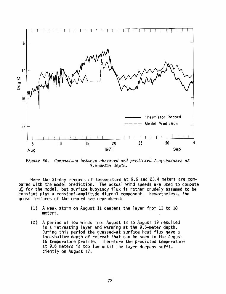
I I

U0>Q)

o

18

15

5Aug

10 15 201971

Thermistor Record

---- Model Prediction

25Sep

4

F-igwr.e. 30. CompaJL.iAon be.:twe.e.n ob.6eJl.ve.d a.nd pfte.cU.ete.d :te.mpeJUttwte..6 at9.6-me.:teJl. de.p:th.

Here the 31-day records of temperature at 9.6 and 23.4 meters are com­pared with the model prediction. The actual wind speeds are used to computeu~ for the model, but surface buoyancy flux is rather crudely assumed to beconstant plus a constant-amplit~de diurnal component. Nevertheless, thegross features of the record are reproduced:

(1) A weak storm on August 11 deepens the layer from 13 to 18meters.

(2) A period of low winds from August 13 to August 19 resultedin a retreating layer and warming at the 9.6-meter depth.During this period the guessed-at surface heat flux gave atoo-shallow depth of retreat that can be seen in the August16 temperature profile. Therefore the predicted temperatureat 9.6 meters is too low until the layer deepens suffi­ciently on August 17.

72

4Sep

3025

Thermistor Record

- - - - Model Prediction

201971

15

between ob.6eJtved a.nd pJtedicted te.mpeJr.a.tuJte..6 at23.4-me.:teJt depth.

18

17

16

u 15 -

C'Q)

0 14

13 -

12

II

105 10

Aug

FigWte 31. Compa.JLi6on

(3) The relatively strong storm of August 20 deepens the layerto over 24 meters and the temperature at 9.6 meters dropsconsiderably. At this time the 23.4-meter thermistor forthe first time lies within the mixed layer and registers thehigher temperature.

(4) Subsequent warming and then cooling after August 30 is dueto another storm. This last storm is nearly as strong asthat of August 20 t but its work is not as obvious becauseit starts with a relatively deep layer.

Figure 32 shows another possible model output--the mixed layer wind­driven current. As shown by Figure 12 t the mean current at the base of themixed layer has only a small effect upon the turbulent energy budget (evenfor Ri* ~ 1). The depth of the mixed layer t on the other hand t directlyinfluences the amplitude of C. Therefore t any surface current predictionrequires knowledge of h(t).

73

II

li

I I I I I! !

17 18 19 20 21 22" ___~ __~ ~__ ~:_ -JI,--_-,':-I_-,i,_--L_--':-_-':----:'_--L_

9 10 II 12 13 14 15 16August 1971

.. L~_~_ .....5 6 7

-10 -

-15- 4

-5 -

15 ~~------'--~--'----T--~T--:----,-~-,------,----r---,----,--~-----,-----,

+V 5Q)

'"......E

FigUILe. 32. A me.lUUlLe. 06 -6e.n.6ib.te. he.at 6.tux at .the. oc.e.a.n -6U1L6ac.e. by bu.oyob-6eJr..vation.6 koWLte.-6Y 06 Vavid Ha.tpeJr..n). 8W( 0) ex: WDoT; W = w<.nd -6pe.e.dat 2 me..teJr..-6 above. -6U1L6ac.e.; DoT = -6U1L6ac.e. wateJr.. .te.mpeJr..atUILe. minu.-6 aJ.Jt.te.mpeJr..atUILe.•

6.7 Evaluation of Model Output

This simulation of a real case is not a strict test of the model. Thesurface buoyancy flux is not known sUfficiently well for this run to be usedeither for calibration purposes or as a test of model behavior.

Inasmuch as the model was designed to have general applicability overall seasons (wide range of values for H*), the proper calibration and testingprocedure requires an integration over a full year. This remains to be doneat a future date under a more operationally-oriented program of research.

Figure 32 shows a measure of the sensible heat flux at the surface (bya bulk parameterization) versus time for the first half of the total periodof observation. (Air temperature was not available after the storm of 21August.) Because relative humidity was not available, the relatively largerlatent heat flux could not be computed. Because the latent heat flux is veryroughly proportional to the sensible heat flux (assuming an approximatelyconstant Bowen ratio), Figure 32 indicates the large magnitude of the net

74

Figwr..e 33. Mea.6wr..ed and p!l..edic.tedp!l..og~~ive vec.to!l.. diag!l..~ 06c.UJr..!l..ent a;t 8.3 me.teJL6 60!l.. twodatj~ 06 :the Ha1.pe!l..n ob~e!l..va.tio~.

8642

01---

2

4

6

VI...Q)+-Q)

Eo

8 r--~----r~---'------'-I---'-l-~~----,

Aug 10 ?:~,

l -;yU911~ ~-

-2 - " '

-4 I~~g12 II -- Current Meter

-6 ,~ ......-:./ Model Prediction;1-- , , I

-8 I-8 -6 -4 -2 0

Ki!ometers

diurnal heat flux compared with the mean daily values. The mean daily heatflux and the diurnal component were assumed to be constant over the entireperiod. This was obviously not true.

Nevertheless, this particular run, as illustrated by Figures 29 to 33,does have didactic value in demonstrating the character of the model re­sponse to realistic boundary conditions. The overall conclusion for thisparticular case is that the wind stress controls the timing of the entrain­ment and retreat events. The degree of surface heating or cooling is impor­tant in determining the extent of the retreat or the deepening. Although theguess at bw(t) was only marginally satisfactory, an important result is thatthe diurnal cycle prescribed gives a much better prediction than does anintegration using a constant heat flux alone.

7. CONCLUS IONS

This model for the ocean mixed layer consists of a number of hypothesesand assumptions regarding the mechanical energy budget, originally shown inFigure 1. In arriving at these hypotheses, mean turbulent field techniqueswere used, but this was done without losing the simplicity of the bulk modelconcept. The particular details of the structure of the mean fields withinthe boundary layer were not of highest priority as a model output. In anycase detailed geophysical data revealing this structure is unavailable totest such a prediction. Of highest importance in this model was the abilityto predict the year-round evolution of the ocean mixed layer depth, togetherwith the bulk properties. There are several models, including those byWyngaard et ale (1974) and Sundararajan (1975), which provide struc~uralpredictions quite nicely, but these boundary layer models are not dlrectly

75

concerned with a changing layer height. An entrainment model is necessary toprovide boundary conditions at the moving density interface.

The atmospheric and oceanic boundary layers present nearly identicalproblems. However, an important difference arises in the surface heat fluxboundary condition. The atmospheric boundary layer is predominantly unstablebecause of minimal absorption of solar radiation within the layer. On theother hand, most of the solar radiation is absorbed near the ocean surfaceand hence turbulent heat flux downward in the oceanic boundary layer is aboutthe same as flux upward in the course of an annual cycle. Therefore, thestable situation is of relatively greater importance in the ocean. As shownby Figures 12 and 14, the nonlinearity of p* (H*) is greatest for H* > 0,the stable region. The treatment of the oceanic case must be made withemphasis upon this point since the linear extrapolation of the unstablesituation will not suffice.

In addition to the nonlinear dependence upon stability, a Rossby numberdependence for the entrainment rate has been found in the nondimensionalsolution, Figure 14. This makes possible a cyclical steady state for theboundary layer without resorting to unrealistic values of upwelling orlateral advection in a long-term integration.

In the short term, on the order of days, the upper ocean, even at higherlatitudes, exhibits significant three-dimensional baroclinic activity. Acase in point is well documented by Gregg (1975) in which only lateral advec­tion can explain the change in heat content after the passage of a storm. Indoing the ensemble or horizontal averaging, such phenomena as well as theshort-period internal waves are treated as noise in the essentially one­dimensional mixed layer dominated by the strong vertical turbulent fluxes ofheat, salt, and momentum. This does not eliminate the practical difficultiesof analyzing and simulating actual observations made at a single point, asshown by the case using real winds to drive the model.

The importance of shorter-period fluctuations in the surface buoyancyflux in modulating the longer-term response has demonstrated the need to knowthe typical daily heating/cooling cycle: Solar radiation, evaporation, con­duction, and back-radiation as a function of season and geographical coordin­ates. The detailed features of this diurnal cycle were not of importance inconducting a qualitative evaluation, but accurate quantitative results froman operational model would be impossible without them. For the same reason,the radiation absorption function should be known. This la~t suggestion maynot be possible without the incorporation of a primary productivity model inwhich case the physics becomes directly dependent upon the biology!

Some of the most fruitful applications of this model lie in the link-upwith other models. The region below the mixed layer has been over a shorttime period successfully treated as a zero-flux "qu iescent abyss." This wasdone primarily for simplicity when the point of focus was the overlyingturbulent boundary layer. The first natural joining of models is betweensuch a boundary layer model with an ocean general circulation model. But whystop there? An atmospheric general circulation model may be combined with

76

the ocean general circulation model--but only through two boundary layer ormixed layer models. It has been demonstrated here that the sea-surface tem­perature, which is so important for weather prediction, cannot be predictedwith accuracy without the proper consideration of the ocean mixed layer.Climate modeling must also pay heed to the oceanic boundary layer. Anomalousevents in the evolution of the mixed layer may induce a delayed response bythe atmosphere when the mi~edliyer again deepens sufficiently.

The interaction between diurnal and annual time scale events has beenparticularly emphasized, but other time scales even longer than a year posesome interesting possibilities, particularly for inactive models.

8. SUMMARY OF MODELED EQUATIONS

ENTRAINMENT BUOYANCY FLUX

-~m4 <w2> <E>

-bw (-h) = h

BUDGET FOR HORIZ. COMPONENTS OF TURB. KINETIC ENERGY

(1)

(2)

_ k: 2ml _ k:<E>2 - -3- «E>2 + fh) <E>

BUDGET FOR VERTICAL COMPONENT OF TURB. KINETIC ENERGY

1 !- (h ;:;z:w ) = h bW(-h) + h bW(O)"2 dt < > 2 2

m ._ ~ -k: 1 -k: -

+ m2 «E> - 3 <\10, » <E>2 - 3 «E>2 + fh) <E>

CONSERVATION OF MEAN BUOYANCY AND MEAN MOMENTUMo

f Q dz-h

77

(3)

(4)

"JUMP CONDITIONS" AT BOTTOM OF MIXED LAYER

- cw (-h) = ~C ~dt

(5)

NOTATION

- bw (-h) = ~B ~dt

C = U + i V

E= u2 + v2 + w2

limL~

( ) dxdy

o

« » = kf ()dz

-h

Ri* = h~B

l~cl2

9. ACKNOWLEDGMENTS

This dissertation and the research leading to it were accomplished withthe assistance and encouragement of many.

Dr. David Halpern, as Chairman of the Supervisory Committee, providedsupport and advice in a manner that permitted the evolution of this work in amost creative atmosphere.

Professors Joost Businger and Frank Badgley, in addition to participat­ing on the Reading Committee, helped lay the foundation of my understandingof turbulent boundary layers. As a visiting professor, Dr. John Wyngaardintroduced me to the techniques of mean-turbulent-field modeling.

78

Dr. Eric Kraus, by inviting me to participate in the N.A.T.O. AdvancedStudy Institute at Urbino in September 1975, gave me the benefit of his owninsight as well as that of other primary workers "in the field at a mostopportune time in the development of this work. Drs. Pearn Niiler andRaymond Pollard were among this group.

Mr. Francis Way must be mentioned because it was he who initiallysteered my interests toward the ocean.

My parents, Roland William and Geraldine Patrick Garwood, have lenttheir support for the longest time. It has been greatly appreciated.

Last, but most of all, thank you to my wife Marilyn. With her supportthis task was made easier, and the entire period was made to be a most en­joyable one.

10. REFERENCES

Arya, S. P. S., and J. C. Wyngaard (1975): . Effect of baroclinicity on windprofiles and the geostrophic drag law for the convective planetaryboundary layer. J. Atmo¢. Sci., 32:767-778.

Benjamin, T. B. (1963): The threefold classification of unstable distur­bances in flexible surfaces bounding inviscid flows. J. Fluid Meeh.,16:435-450.

Businger, J. A. and S.P.S. Arya (1974): Height of the mixed layer in thestably stratified planetary boundary layer. Adv. ~n Geophy¢., 18A,Academic Press, New York, 73-92.

Businger, J. A., J. C. Wyngaard, Y. Izumi, and E. F. Bradley (1971): Flux­profile relationships in the atmospheric surface layer. J. Atmo¢. S~.,

28:181-189.

Denman, K. L. (1973): A time-dependent model of the upper ocean. J. Phy¢.Oeean., 3:173-184.

Ekman, V. W. (1905): On the influence of the earth1s rotation on oceancurrents. ~k. Mat. A¢~on. Fy¢., 2(11):1-53.

Farmer, D. M. (1975): Penetrative convection in the absence of mean shear.Quant. J. R. Met. Soe., 101:869-891.

Geisler, J. E. and E. B. Kraus (1969): The well-mixed Ekman boundary layer.Veep-Sea R~., Suppl., 16:73-84.

Gill, A. E. and P. P. Niiler (1973): The theory of seasonal variability inthe ocean. Veep-Sea R~., 20:141-177.

79

Gregg, M. C. (1975): Fine and microstructure observations during the passageof a mild storm. (Unpublished manuscript).

Halpern, D. (1974): Observations of the deepening of the wind-mixed layer inthe northeast Pacific Ocean. J. Phy~. Oeean., 4 (3): 454-466.

Kantha, L. H. (1975): Turbulent entrainment at the density interface of atwo-layer stably stratified fluid system. Department of Earth andPlanetary Science Technical Report No. 75-1. Johns Hopkins University,Baltimor~, 162 pp.

Kato, H. and O. M. Phillips (1969): On the penetration of a turbulent layerinto stratified fluid. J. Fluid Meeh., 37:643-655.

Kitaigorodsky, S. A. (1960): On the computation of the thickness of thewind-mixing layer in the ocean. Bull. Aead. Sci. U.S.S.R., GeophY~.

SVl.., 3: 284-287 •

Kraus, E. B. and C. Rooth (1961): Temperature and steady state vertical heatflux in the ocean surface layers. Tettuh, 13: 231-238.

Kraus, E. B. and J. S. Turner (1967): A one-dimensional model of the sea­sonal thermocline, part II. TellU6, 19:98-105.

Lamb, H. L. (1932): Hy~dynami~. Dover, New York, 738 pp.

Long, R. R. (1974): The influence of shear on mixing across density inter­faces. (Unpublished manuscript).

Lumley, J. L. and B. Khajeh-Nouri (1973): Computational modeling of turbu­lent transport. Adv. ~n Geophy~., 18A, Academic Press, New York, 169­192.

Mellor, G. L. and H. J. Herring (1973): A survey of the mean turbulent fieldclosure models. A1AA Jo~nal, 11 (5):590-599.

Miropol 'skiy, Yn. A. (1970): Nonstationary model of the wind-convectionmixing layer in the ocean. liv., Atm. and Oeean Phy~., 6(12):1284-1294.

Moore, J. M. and R. R. Long (1971): An experimental investigation of turbu­lent stratified shearing flow. J. Fluld Meeh., 49: 635-655.

Munk, W. and E. R. Anderson (1948): Notes on a theory of the thermocline.J. M~. R~., 7:276-295.

Niiler, P. P. (1975): Deepening of the wind-mixed layer. J. M~. R~.,

33(3):405-422.

Pollard, R. T. and R. C. Millard, Jr. (1970): Comparison between observedand simulated wind-generated inertial oscillations. Veep-Sea R~.,

17:813-821.

80

Pollard, R. T., P. B. Rhines and R. O. R. Y. Thompson (1973): The deepeningof the wind-mixed layer. Geophif~. Fluid Vyn., 3:381-404.

Rossby, C. G. and R. B. Montgomery (l935): The layer of frictional influencein wind and ocean currents. Papers Phys. Oceanog. and Meteorol., MITand Woods Hole Oceanogr. Inst., 3 (3):101 pp.

Rotta, J. C. (1951): Statistische Theorie Nichthomogener Turbulenz. Z. 6u~

Phif~~k, 129:547-572.

Sundararajan, A. (1975): Significance of the neutral height scale for theconvective, barotropic planetary boundary layer. J. Atmo~. Sci.,32(12):2285-2287.

Tennekes, H. and J. L. Lumley (1972): A F~t Co~e ~ T~bulence. MITPress, Cambridge, Mass. 300 pp.

Tennekes, H. (1973): A model for the dynamics of the inversion above aconvective boundary layer. J. Atmo~. Sci., 30:558-567.

Thompson, R. (l974): Predicting the characteristics of the well-mixed layer.Woods Hole Ocean. Inst. Tech. Report, 76pp.

Turner, J.S. (1968): The influence of molecular diffusivity on turbulententrainment across a density interface. J. Fluid Mech., 33:639-656.

Turner, J. S. (1969): A note on wind-mixing at the seasonal thermocline.Veep-Sea R~., 16:Suppl., 297-300.

Wyngaard, J. C., O. R. Cot~ and K. S. Rao (1974): Modeling of the atmos­pheric boundary layer. Adv. ~n Geophif~. 18A:193-212.

81

1< u.s. Government Printing Office: 1977-777-045/1225 Region 8