A GENERAL METHOD FOR SIZING BATTERY ENERGY STORAGE SYSTEMS

A GENERAL METHOD FOR SIZING BATTERY ENERGY STORAGE SYSTEMS FOR

USE IN MITIGATING PHOTOVOLTAIC FLICKER

_______________________________________

A Thesis

presented to

the Faculty of the Graduate School

at the University of Missouri-Columbia

_______________________________________________________

In Partial Fulfillment

of the Requirements for the Degree

Master of Science

_____________________________________________________

by

WILLIAM NOAH WILLS

Dr. John Gahl, Thesis Supervisor

July 2017

© Copyright by William Noah Wills 2017

All Rights Reserved

The undersigned, appointed by the dean of the Graduate School, have examined the thesis entitled

A GENERAL METHOD FOR SIZING BATTERY ENERGY STORAGE SYSTEMS FOR

USE IN MITIGATING PHOTOVOLTAIC FLICKER

presented by William Noah Wills,

a candidate for the degree of master of science,

and hereby certify that, in their opinion, it is worthy of acceptance.

Professor John Gahl

Professor Robert O’Connell

Professor William H. Miller

ii

Acknowledgements

William Wills would like to thank his examining committee, who at different points in his

academic career have each provided him guidance and help, those involved in the STEPS

Fellowship program at MU, and those at Ameren who have provided assistance to this

work, specifically Randy Schlake and Greg Palmer.

iii

Table of Contents

Acknowledgements ........................................................................................................... ii

Table of Figures................................................................................................................ vi

Table of Tables ................................................................................................................ vii

Abstract: ........................................................................................................................... ix

1 Introduction ............................................................................................................... 1

1.1 Utility-scale PV Issues ........................................................................................ 2

1.2 Flicker ................................................................................................................. 2

1.3 Battery Energy Storage Systems ......................................................................... 4

1.4 Description of Problem ....................................................................................... 4

2 Literature Review ..................................................................................................... 5

2.1 General Texts on PV Flicker ............................................................................... 5

2.1.1 IEEE Recommended Practice for the Analysis of Fluctuating Installations on

Power Systems [5] ...................................................................................................... 5

2.1.2 J. Hernandez, M. Ortega, and P. Vidal [11] .................................................... 7

2.1.3 Y. S. Lim and J. H. Tang [12] ......................................................................... 7

2.1.4 S. Zhu, J. Zhang, X. Qin, and C. Niu [13] ...................................................... 8

iv

2.2 Texts Specific to BES Use for PV Flicker .......................................................... 8

2.2.1 IEEE Recommended Practice for Sizing Nickel-Cadmium Batteries for

Photovoltaic (PV) Systems [14].................................................................................. 8

2.2.2 W. Jin, Z. Xie, and B. Li [15] ......................................................................... 9

2.2.3 M. Z. Daud and A. Mohamed [16] ............................................................... 11

2.3 Texts Concerning Battery Lifetime Prediction ................................................. 12

2.3.1 D. U. Sauer, J. Schiffer, et al ........................................................................ 13

2.3.2 R. Dufo-López, J. M. Lujano-Rojas, J. L. Bernal-Agustín [28] ................... 13

3 Method ..................................................................................................................... 14

3.1 Design Day Characterization ............................................................................ 14

3.2 Determination of Expected Flicker Severity ..................................................... 15

3.3 Determination of Battery Requirement ............................................................. 15

3.4 Battery Type Analysis....................................................................................... 18

3.5 Economic Analysis ........................................................................................... 19

4 Case Study ............................................................................................................... 23

4.1 Problem Overview ............................................................................................ 23

4.2 Design Day Characterization ............................................................................ 23

4.3 Determination of Expected Flicker Severity ..................................................... 24

4.4 Determination of Battery Requirement ............................................................. 26

4.5 Economic Analysis ........................................................................................... 28

5 Conclusion ............................................................................................................... 32

5.1 Cost Issues ........................................................................................................ 32

v

5.2 General Limitations of the Method ................................................................... 32

5.3 Alternative Solutions ........................................................................................ 33

5.4 Further Research ............................................................................................... 34

Reference Documents ..................................................................................................... 35

vi

Table of Figures

Figure 1.1 - GE Flicker Curve ............................................................................................ 3

Figure 2.1 - Statistical graph of 1 minute and 10 minutes time interval ............................. 9

Figure 2.2 - Statistical graph of all BESS power (“Fig. 5” in [6]) .................................... 10

Figure 2.3 - The curves of BESS energy change (“Fig. 6” in [6]) .................................... 11

Figure 2.4 - SOC-FB control scheme for BES (“Fig. 3” in [7]) ....................................... 12

Figure 3.1 - GE Flicker Curve with Flicker Values .......................................................... 17

Figure 3.2 - DoD vs. Number of Cycles for Lead-acid and Lithium-ion Batteries .......... 19

Figure 4.1 - Percent Voltage Deviation vs. Solar Power Deviation ................................. 27

vii

Table of Tables

Table 3.1 - Parameters and Terms .................................................................................... 14

Table 3.2 - DoD vs. Number of Cycles for Lead-acid and Lithium-ion Batteries ........... 18

Table 3.3 - Cost Information for Lead-acid and Lithium-ion Batteries ............................ 21

Table 3.4 - Economic Analysis Template ......................................................................... 22

Table 4.1 - Statistics on Solar Activity ............................................................................. 25

Table 4.2 - Design Day Parameters .................................................................................. 26

Table 4.3 - Power Flow Analysis Results ......................................................................... 26

Table 4.4 - BES System Parameters ................................................................................. 27

Table 4.5 - Economic Analysis for Lead-acid Batteries for High-end Capital and Low-end

O&M Costs ....................................................................................................................... 28

Table 4.6 - Economic Analysis for Lead-acid Batteries for High-end Capital and High-end

O&M Costs ....................................................................................................................... 28

Table 4.7 - Economic Analysis for Lead-acid Batteries for Low-end Capital and High-end

O&M Costs ....................................................................................................................... 29

Table 4.8 - Economic Analysis for Lead-acid Batteries for Low-end Capital and Low-end

O&M Costs ....................................................................................................................... 29

Table 4.9 - Economic Analysis for Lithium-ion Batteries for High-end Capital and High-

end O&M Costs ................................................................................................................ 30

Table 4.10 - Economic Analysis for Lithium-ion Batteries for High-end Capital and Low-

end O&M Costs ................................................................................................................ 30

Table 4.11 - Economic Analysis for Lithium-ion Batteries for Low-end Capital and High-

end O&M Costs ................................................................................................................ 31

viii

Table 4.12 - Economic Analysis for Lithium-ion Batteries for Low-end Capital and Low-

end O&M Costs ................................................................................................................ 31

ix

Abstract:

A method for sizing battery energy storage (BES) systems for use in mitigating voltage

flicker caused by solar intermittency in photovoltaic generation was developed. The

method creates a “design day” from existing solar data and designs the power and

energy requirements for a BES system that can help a photovoltaic facility mitigate

flicker caused by solar activity associated with the design day. An economic analysis

of lead-acid and lithium-ion options for the BES was also developed. The method was

then applied to a proposed photovoltaic project in the Midwestern United States.

1

1 Introduction

Renewable energy technology is advancing, with the share of energy generation from

renewable sources growing[1]. One renewable energy type that has caught the public

imagination is solar power, particularly in the form of photovoltaics (PV). Photovoltaics

(PV) cells directly convert solar energy into electrical energy by taking advantage of

photon and electron interactions in semi-conductive materials in a process that works in

the reverse of that of light emitting diodes [2].

PV systems have many different applications, from powering small electronic devices to

residential use to utility-scale grid-connected generation. PV systems are often used with

batteries to store generated electricity. Residential PV use, so called “rooftop” solar, is

becoming increasingly popular for its ability to offset electricity costs and for its

environmental friendliness.

PV generation can be both off-grid, or “islanded,” and grid-connected. Islanded generation

refers to set-ups where the PV resources are not connected to the local electric utility’s

other generation and transmission resources. Grid-connected PV resources can include

rooftop solar as well as utility-scale projects overseen by electric utility companies. These

utility-scale projects can be in the megawatt range, much larger than rooftop solar projects.

PV generation does present certain challenges, however. For starters, it depends on solar

irradiance, which is only available for part of the day, and can be undependable due to the

climate and weather conditions. While PV can generate energy when clouds are overhead,

solar intermittency caused by moving clouds can cause rapid changes in power. For grid-

connected PV use, this can cause power quality issues [3].

2

These challenges extend to rooftop solar power as well. Rooftop solar, even when it is

grid-connected, is not directly controlled by utilities. Some utilities may want to avoid

power quality issues coming from rooftop solar because of this and build their own solar

resources. While this means that utilities can serve customers’ desire for solar power, it

also means that utilities must deal with power quality issues stemming from solar

intermittency.

1.1 Utility-scale PV Issues

Intermittent solar activity disrupts PV generation. For grid-connected, utility-scale PV

installations, this is not necessarily a problem, because utilities generally have other

sources of electricity generation. However, the intermittency can cause fast-ramping

voltage excursions. These voltage deviations can cause flicker (discussed below) and stress

on substation equipment.

One key piece of equipment involved in this issue is the load tap changer (LTC). LTCs

adjust the turns ratio on substation transformers, allowing the electrical grid to respond to

changes in generation and load[4]. LTCs are particularly important in grid-connected PV

installations (both rooftop and utility-scale). One of the consequences of solar

intermittency is that LTCs serving PV installations can suffer from overuse by responding

to the sometimes-rapid changes in generation.

1.2 Flicker

For utility customers, voltage deviation manifests itself as a flickering of incandescent

lights, hence voltage deviation is called “flicker.”[5] The acceptability of voltage flicker

is measured by the GE Flicker Curve, an industry tool, seen in Figure 1.1. It plots percent

voltage change ("flicker") against frequency of deviations, and has two curves on it, one

3

representing flicker visible by humans and one representing flicker that is irritable to

humans. These curves are based on industry research and used based on electric utility

industry convention rather than law. [6]

Voltage deviation has always been an issue in electrical grids. Between the 1920’s and the

1950’s, several studies on voltage deviation perception were performed and culminated in

flicker curves developed by General Electric (GE) and Consolidated Edison (Con Ed)[6].

GE’s curve is today widely used in the utilities industry and used in the Institute of

Electrical and Electronics Engineers’ (IEEE) standards ([7, 8]) as a guide to what amount

of voltage deviation in the customer’s electric supply is likely to cause customer irritation

and complaint.

Figure 1.1 - GE Flicker Curve

4

It should be noted that the GE Flicker Curve assumes incandescent lightbulb use. Per the

Energy Independence and Security Act of 2007 (EISA), incandescent lightbulb use has

been severely limited. Among other standards, the Act bans the manufacture of household

incandescent lightbulbs due to their inefficiency [9, 10]. Because the GE Flicker Curve is

based on incandescent lamps, and because electric utilities typically use the Curve as their

flicker limit, utilities may be using an inaccurate and non-useful tool for flicker standards.

However, the GE Flicker Curve is still the industry standard, and is used throughout this

work.

1.3 Battery Energy Storage Systems

One possible solution to flicker caused by solar intermittency in PV generation is to use

battery energy storage (BES) to help support the PV installations. Battery energy storage

systems (BESS) can be connected to PV installations to “fill in” the gaps in generation

caused by solar intermittency. The BESS would be discharged as needed and recharged

regularly. These BESS would need to be scalable up to the megawatt-hour range, be

capable of fast and repeatable discharges, and have a long lifetime (that is, capable of

several discharges and recharges).

1.4 Description of Problem

In this work, the problem studied will be how to mitigate voltage flicker that is caused by

solar intermittency in photovoltaic installations. The method chosen will be to use battery

energy storage systems. The main goals will be to prevent flicker in customer loads and to

relieve stress and maintenance costs on equipment, particularly load tap changers.

5

2 Literature Review

This literature review seeks to detail extant industry practices associated with smoothing

of utility scale photovoltaic facility output. Two groups of works were reviewed: literature

related to general analysis of PV flicker, and literature related to using BES systems for

PV flicker mitigation. For literature related to general analysis of PV flicker, [5, 11-13]

were the main works reviewed. For literature related to using BES systems to mitigate PV

flicker, [14-16] were the main works reviewed. [3, 17-20] and [8, 21-25] were reviewed

but determined to not be of immediate use.

2.1 General Texts on PV Flicker

The following is an analysis of the relevant elements of the four texts ([5, 11-13]) that deal

with general analysis of PV flicker that were most important or useful in the investigation

so far.

One IEEE standard was found, [5], that includes tools for the analysis of PV flicker. Other

works ([11-13]) draw upon the analysis tools in the standard, expand upon those tools, and

show the broad usage of the standard’s analysis tools.

2.1.1 IEEE Recommended Practice for the Analysis of Fluctuating Installations on

Power Systems [5]

The standard is concerned with the practice of measuring and analyzing voltage flicker

present in power systems. Many practices in the standard are descended from international

standards, particularly from the International Electrotechnical Commission (IEC).

6

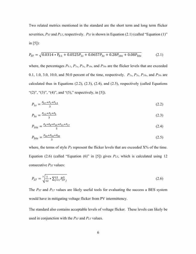
Two related metrics mentioned in the standard are the short term and long term flicker

severities, PST and PLT, respectively. PST is shown in Equation (2.1) (called “Equation (1)”

in [5]):

0.0314 ∗ P . 0.0525 0.0657 0.28 0.08 (2.1)

where, the percentages P0.1, P1s, P3s, P10s, and P50s are the flicker levels that are exceeded

0.1, 1.0, 3.0, 10.0, and 50.0 percent of the time, respectively. P1s, P3s, P10s, and P50s are

calculated thus in Equations (2.2), (2.3), (2.4), and (2.5), respectively (called Equations

“(2)”, “(3)”, “(4)”, and “(5),” respectively, in [5]).

. . (2.2)

. (2.3)

(2.4)

(2.5)

where, the terms of style PX represent the flicker levels that are exceeded X% of the time.

Equation (2.6) (called “Equation (6)” in [5]) gives PLT, which is calculated using 12

consecutive PST values:

∗ ∑ (2.6)

The PST and PLT values are likely useful tools for evaluating the success a BES system

would have in mitigating voltage flicker from PV intermittency.

The standard also contains acceptable levels of voltage flicker. These levels can likely be

used in conjunction with the PST and PLT values.

7

The standard includes the GE Flicker Curve (Figure 1.1, called “Fig. 1” in [5]).

2.1.2 J. Hernandez, M. Ortega, and P. Vidal [11]

The paper summarizes the state of knowledge on analyzing PV distributed generation

issues, including flicker. The paper mentions the PST and PLT values mentioned in [5]. It

should be noted that the paper is written with the assumption of International

Electrotechnical Commission (IEC) standards (and thus not IEEE). However, the fact that

the PST and PLT values have broad usage gives weight to their usefulness.

2.1.3 Y. S. Lim and J. H. Tang [12]

The paper details an experiment to study the effects of PV intermittency on voltage flicker

in Malaysia, a country particularly susceptible to PV intermittency. The paper also

proposes a solution to PV flicker in the form of a dynamic load controller.

The paper uses the PST and PLT values and generalizes them, as shown in Equations (2.7)

and (2.8) (called Equations “(2)” and ”(3),” respectively, in [12]), to:

∗ (2.7)

where d is the average number of voltage changes in a minute and d0 is the relative voltage

change that produces PST0 = 1.0.; and:

∑ (2.8)

The paper also explains the near linear relationship between change in PV power output

and voltage change.

8

2.1.4 S. Zhu, J. Zhang, X. Qin, and C. Niu [13]

The article evaluates new testing techniques for evaluating flicker, harmonics, inter-

harmonics, and high frequency components in large scale PV installations connected to

medium-voltage grids in China. The article’s method of analysis involves a “fictitious

grid”. This analysis includes a version of the PST value, as shown in Equation (2.9):

,, (2.9)

where PST,fic is the flicker emission value of a fictitious grid, SK,fic is the three-phase short

circuit apparent power of the fictitious grid, and Sn is the rated apparent power of PV

station. This version of the PST value draws from the IEC standard that [5] is a counterpart

to.

2.2 Texts Specific to BES Use for PV Flicker

The following is an analysis of the relevant elements of the three texts ([14-16]) that relate

to BES use for PV flicker that were most important or useful in the investigation so far.

None of the reviewed works directly answered the study’s objective. There is one

withdrawn IEEE standard, [14], that relates directly to the study’s objective. [15] and [16]

address BES sizing while discussing BES control methods.

2.2.1 IEEE Recommended Practice for Sizing Nickel-Cadmium Batteries for

Photovoltaic (PV) Systems [14]

No documentation on why the standard was withdrawn could be obtained. However, the

standard’s method for determining battery size is based on the assumption that the battery

is to be used to support the load when the PV cannot. It is assumed that the standard was

discontinued because it does not address battery use in solar intermittency.

9

None of the current IEEE standards related to BES use in photovoltaic intermittency

mitigation cover grid-connected systems.

2.2.2 W. Jin, Z. Xie, and B. Li [15]

The article analyses a PV installation in China and determines an appropriate BES system

and control strategy to mitigate voltage flicker.

Section II of the article indicates that there is a standard requirement in China that power

variation in PV power be analyzed in 1 minute and 10 minute intervals. This is seen

throughout the paper.

Section III of the article deals with BES capacity. The general approach is to find the

power requirement and the energy capacity requirement for the BES.

Figures Figure 2.1 and Figure 2.2 (Figures “4” and “5” in [15]) deal with the power

requirement. Figures Figure 2.1 and Figure 2.2 show power values versus the percentage

of the time that power value occurs. Figure 2.1 is the one minute and 10 minute values and

Figure 2.2 is the combined one minute and 10 minute values. Both figures have a near

Figure 2.1 - Statistical graph of 1 minute and 10 minutes time interval

BESS power output statistics (“Fig. 4” in [6])

10

normal distribution around zero. The BES power requirement is then the range of Figure

2.2, 10MW.

Figure 2.3 (“Fig.6” in [15]) presents the energy vs. time graphs for each interval. From

Figure 2.3, the paper derives the energy ranges [E0-3.12, E0+0.54] and [E0-15.14, E0] for

the 1 minute and 10 minute intervals, respectively, where E0 is the initial value of the BES.

A state of charge range is given as [20%, 80%]. The paper then presents 6.10 MWh and

25.23 MWh as the BES energy capacity (termed Ecap here) for the 1 minute and 10 minute

intervals, respectively. The values for Ecap seem to be derived from:

.

. .25.23

and

. .

. .6.10

More generally, for energy range [E0-Em, E0+ En] and state-of-charge range [rmin, rmax], Ecap

and E0 are:

(2.10)

∗ ∗ (2.11)

Figure 2.2 - Statistical graph of all BESS power (“Fig. 5” in [6])

11

The power values in Figures Figure 2.1 and Figure 2.2 appear to be the difference between

PV power and grid power, while Figure 2.3 appears to show the difference between the PV

energy generation and the grid energy consumption. Since Figure 2.3 shows the energy

value increasing and decreasing, it is concluded that the figures show a difference in energy

and power consumption or generation.

2.2.3 M. Z. Daud and A. Mohamed [16]

The paper is concerned with a control method for a PV/BES system. The method has three

modes of operation. “Mode I” is the grid-connected low fluctuation mode, shown in

Equation (2.12) (called “Equation (1)” in [16]):

, – (2.12)

where PG,ref is the grid power, PPV is the photovoltaic power and PL is the load power.

“Mode II” is the grid-connected high fluctuation mode, shown in Equation (2.13) (called

“Equation (2)” in [16]):

, – (2.13)

Figure 2.3 - The curves of BESS energy change (“Fig. 6” in [6])

0 10 20 30

E0-3

E0-2

E0-1

E0+1

time/day(a)

0 10 20 30

E0-15

E0-10

E0-5

time/day(b)

E0

E0

12

where PSET is the power smoothing set point and PBES,ref is the reference power discharged

from the BES. “Mode III” is the emergency mode, including non-grid connected mode.

Non-grid connected mode is given by Equation (2.14) (called “Equation (3)” in [16]):

, – (2.14)

The remaining energy level (REL) is the feedback signal used to control the BES state of

charge. REL is given by Equation (2.15) (called “Equation (4)” in [16]):

dt (2.15)

where CBES is the BES capacity. Figure 2.4 (called “Fig. 3” in [16]) gives the control

scheme. The scheme includes the parameters TSOC, the SOC time constant, M, the SOC

margin rate, and α, a coefficient defined by Equation (2.16) (called “Equation (5)” in [16])

as:

(2.16)

2.3 Texts Concerning Battery Lifetime Prediction

The following is an analysis of the relevant elements of the three texts ([26-28]) that deal

with battery lifetime prediction. While battery lifetime prediction is addressed in Section

3.5, the method described is very basic. The texts discussed in this section are sophisticated

Figure 2.4 - SOC-FB control scheme for BES (“Fig. 3” in [7])

13

treatments of battery lifetime prediction, but out of the scope of this project. More

sophisticated battery lifetime prediction is a good “next step” for this project, as potential

battery lifetimes inform BESS purchases and projects.

2.3.1 D. U. Sauer, J. Schiffer, et al

Of interest is the work of D. U. Sauer et al., whose body of work involves battery use in

renewable energy systems. Sauer’s more recent work, particularly [26, 27], involves

lifetime prediction for battery energy systems.

Sauer et al.’s prediction model is based on the internal battery chemistry, specifically the

grid corrosion on the positive electrode and the degradation of the active material. The

model also takes into account acid stratification, gassing, and the lead sulfate crystal

structures. The model continuously multiplies the Ah throughput by a weight factor based

on depth-of-discharge, current rate, existing acid stratification, and the time since the last

charging.[27]

2.3.2 R. Dufo-López, J. M. Lujano-Rojas, J. L. Bernal-Agustín [28]

The work evaluates three different battery lifetime prediction models, including Sauer et

al.’s ([27]). The three models are the Equivalent Full Cycles to Failure, Rainflow Cycle

Counting, and the Weighted Ah-throughput (Sauer et al.’s model). The work uses each

method to predict the battery lifetime of two battery systems, an off-grid household PV

system, and an alarm system, and compares the predicted lifetime with the actual lifetime

of the two systems. The work finds that Sauer’s model is the most accurate model.

14

3 Method

The described method consists of characterizing a “design day,” determining the expected

level of flicker the system will experience during the design day, determining what power

and energy requirements are needed to mitigate the expected flicker, and determining the

most economical battery type to use.

Table 3.1 shows the parameters and terms that will be used throughout.

3.1 Design Day Characterization

The “design day” is the hypothetical day that a BES system supporting a photovoltaic

station must be designed to accommodate. It represents a “worst case” scenario while still

being possible. The design day is derived from solar data taken in the area of the PV

Table 3.1 - Parameters and Terms Term Description Units Note

V Percent voltage deviation % PPV Solar power deviation MW VR Expected flicker % Pd Design day power value MW VR Flicker that is mitigated %

VC Percent voltage change at design day

frequency %

Using GE Flicker Curve

b Acceptable point below flicker curve % Using GE Flicker

Curve PR Battery Power requirement MW

Cnominal Nominal battery energy requirement MW-h fd Design day frequency Hour-1 Td Design day dip duration hour

Cactual Actual needed battery energy requirement MW-h d Design depth of discharge % L End of life depth of discharge %

nex Expected number of recharge cycles - dex Expected depth of discharge % Cex Expected daily energy usage MW-h

15

facility. The design day parameters are the dip depth (Pd), the dip frequency (fd), and the

dip duration (Td). Appropriate, predictive statistical analysis is used to determine

reasonable values for the design day characteristics.

3.2 Determination of Expected Flicker Severity

Power flow analysis is done to find the relationship between the solar power deviation and

the percent voltage deviation in the load, and thus the expected magnitude of the voltage

flicker. This analysis can yield a polynomial approximation of the relationship between

the solar power deviation, and the percent voltage deviation. Equation (1) shows the

relationship in the form of an n degree polynomial:

∆ ∗ ∗ ⋯ 1

where V is the percent voltage deviation, PPV is the solar power deviation, and an is a

constant. Equation (1) can be used with a power value to calculate the corresponding

flicker value, and vice-versa, as will be seen in the next section.

3.3 Determination of Battery Requirement

The expected flicker level, VR, and the design day frequency, fd, are compared to the flicker

curve (Figure 1.1) to determine the acceptability of the expected flicker. If the expected

flicker is above the flicker curve at the design day frequency, the flicker is determined to

be unacceptable. An acceptable flicker level is then chosen below the flicker curve at the

design day frequency per Figure 1.1.

It should be noted that here, “flicker curve” refers to either the visibility curve or the

irritability curve on Figure 1.1, depending on the engineer’s preference. While flicker

16

above the irritability curve must be mitigated, some utilities may find that any visible

flicker will cause customer complaints.

VR is calculated using Equation (2), which is derived from Equation (1):

∆ ∗ ∗ ⋯ (2)

where Pd is the design day power value.

VR is the flicker amount that needs to be mitigated. It is a percent voltage change

represented by Equation (3).

∆ ∗ (3)

where VC is the percent voltage change on the flicker curve at the design day frequency,

and b is the threshold (in percent) below the flicker curve that is chosen to be mitigated.

The battery power requirement, PR, is calculated by Equation (4) (derived from Equation

(1)).

∗ ∗ ⋯ (4)

Figure 3.1, using example values, illustrates the relationship between VR, VC, VR, and the

flicker curve. In this example, a 5% voltage deviation at a frequency of 5 dips per minute

is mitigated to 90% of the visibility curve. This yields a VR value of 3.65%.

For the nominal battery energy requirement, Cnominal, the power requirement, PR, is

multiplied by the design day values for dip frequency (fd), the dip duration (Td), and the

number of hours observed in a day, given by Equation (5):

∗ ∗ ∗ (5)

17

It should be noted that the time component of Cnominal is not limited by how fast the LTC

moves. The amount of time the LTC needs to move (and thus when power from elsewhere

in the grid can be drawn) is the shortest amount of time that flicker support can be used.

Thus, one might expect the LTC movement time to be used as the time component in

Cnominal so that the energy value can be minimized. However, part of the goal of the method

is to relieve maintenance costs on the LTC. By basing Cnominal on the length of the expected

dip, the LTC does not need to move as fast, and thus stress and maintenance costs on the

LTC can be minimized.

Figure 3.1 - GE Flicker Curve with Flicker Values

18

3.4 Battery Type Analysis

For every recharge cycle, battery capacity degrades based on the depth of discharge (DoD)

of each recharge cycle[29]. Each battery type has an “end-of-life” capacity after which it

is no longer considered usable (per industry convention) [29-31] .

To calculate a battery’s actual needed capacity, the nominal capacity is divided by a chosen

DoD and divided by the percent capacity that is considered the “end-of-life” for that battery

chemistry (this ensures that the battery has the requisite capacity at the end-of-life):

∗ (6)

where d is the chosen DoD (in percent) and EoL is the percent capacity that is considered

end-of-life for the battery type (in percent). The chosen DoD, d, will depend on the desired

number of recharge cycles before the BES capacity falls below the end-of-life capacity.

For lead-acid and lithium-ion batteries, the end-of-life capacity is 80% [29-31]. Figure 3.2

shows the relationship between DoD and number of recharge cycles for lead-acid and

lithium-ion (specifically lithium iron phosphate) batteries, while Table 3.2 tabulates that

data[31, 32].

Table 3.2 - DoD vs. Number of Cycles for Lead-acid and Lithium-ion Batteries DoD (d) Lead-acid Lithium-ion 100.0% 500 968 90.0% 590 1198 80.0% 675 1519 70.0% 780 1990 60.0% 950 2716 50.0% 1150 3925 40.0% 1475 6158 30.0% 2050 11008 20.0% 3300 24960 10.0% 7000 101163

19

3.5 Economic Analysis

The Equivalent Uniform Annual Cost (EUAC) is used to analyze the project. The EUAC

distributes the lifetime cost of the project over each year and is sometimes referred to as

the “annual worth” of a project[33]. For this project, the EUAC is the sum of the annual

maintenance costs, the product of the up-front cost and an interest factor representing the

annual value given the up-front cost, and the product of the up-front cost and an interest

factor representing the annual value given the future cost. Equation (7) shows the formula

for the EUAC:

∗ ⁄ | | ∗ ⟨ ⁄ | | ⟩ (7)

where the bracketed terms are the interest factors, P is the up-front cost, M is the yearly

operation and maintenance cost, i is the interest rate, nl is the number of interest periods (in

years) for the total lifetime of the project, and nr is the number of interest periods (in years)

for each battery replacement (if needed). The first term represents the equivalent annual

Figure 3.2 - DoD vs. Number of Cycles for Lead-acid and Lithium-ion Batteries

y = 517.78x‐1.162

y = 968.28x‐2.019

100

1000

10000

100000

1000000

10000000

0% 10% 20% 30% 40% 50% 60% 70% 80% 90% 100%

Num

ber

of R

echa

rge

Cyc

les

Depth of Discharge

Lead‐acid

Lithium‐ion

20

value of the up-front cost taken over the entire lifetime of the project. The second term

represents the equivalent annual value of the battery replacements costs (if such

replacements are needed).

The up-front cost, also called “capital” or “principal” cost, is calculated by multiplying the

battery energy requirement by the per kilowatt-hour capital cost for that battery type:

∗ ∗ (8)

Likewise, the yearly operation and maintenance (O&M) cost is calculated by multiplying

the battery energy requirement by the per kilowatt-hour yearly operation and

maintenance cost for that battery type:

∗ & ∗ (9)

The number of interest periods for each replacement is the number of expected recharge

cycles for the chosen BESS divided by the number of recharges in a year, which is also the

number of days in the year that the BESS is used:

# (10)

where nex is the expected number of recharge cycles for the replacement period. It is

assumed that the BESS will be recharged every day it is used. However, this does not

mean that the number of days used in a year is 365. Depending on climate, solar

intermittency may only cause power dips (and thus voltage deviation) during part of the

year. This is because power demand from utility customers often follows seasonal patterns.

It may be that customers demand more power than PV resources can provide (particularly

in the Winter), thus solar power deviations will not affect customers (that is, power is being

drawn from elsewhere in the grid). It may also be that customers demand so little power

21

compared to PV resources that no amount of day-time solar intermittency will affect

customers. Power flow analysis (like that mentioned in Section 3.2) must take into account

during what part of the year PV generation and customer demand are close enough for solar

intermittency to be a problem.

The number of battery system replacements will be the total project lifetime divided by the

replacement time period:

(11)

The expected discharge can be used to determine the expected number of recharge cycles,

nex, using a DoD vs. number of recharge cycles chart (such as Figure 3.2). The expected

discharge, dex, is:

(12)

where Cex is the expected daily energy usage. For this work, Cex will be assumed to be the

average daily energy loss due to dips.

Table 3.3 shows the low-end and high-end costs associated with lead-acid and lithium ion

batteries for distribution substation uses (a similar use to the project described herein) [34].

Once the above values are calculated, a table using Table 3.4 as a template can be made

and used to make economic decisions. Tables Table 4.5 through Table 4.12 (in Section

4.5) use Table 3.4 as a template.

Table 3.3 - Cost Information for Lead-acid and Lithium-ion Batteries

Battery Type

Low-end Capital Cost

($/kW*h)

High-end Capital Cost

($/kW*h)

Low-end Operation and Maintenance

Cost ($/kW*h /year)

High-end Operation and Maintenance

Cost ($/kW*h /year) Lead-acid 511 1211 12 28

Lithium-ion 432 901 7 14

22

Table 3.4 - Economic Analysis Template

DoD (d) Battery

Capacity (Cactual)

Expected Discharge rate, dex

Expected recharge cycles, nex

Replacements over 30-year lifetime

Capital Cost O&M Costs

EUAC

100.0% - - - - - - -

90.0% - - - - - - - … … … … … … … …

23

4 Case Study

4.1 Problem Overview

A utility-scale, grid-connected 13.5 MW photovoltaic facility is proposed to serve in the

Midwestern United States. The electric utility proposing the project (henceforth “Utility”)

is concerned that solar intermittency at the facility may cause voltage flicker in the

customers served by the facility.

4.2 Design Day Characterization

Data on solar dips at an existing 4.5 MW solar PV installation were collected by the Utility

between June and September of 2015. This facility is in the same area as the proposed

project and is also owned by the Utility, thus the data can be used to predict solar behavior

at the proposed facility. Table 4.1 shows these data and the various statistics associated

with dip behavior. These data are used as the basis of the design day for the proposed solar

facility. It should be noted that the distributions for dip depth, and dip frequency are near-

normal distributions (that is, their distributions approximately follow a “bell curve” shape).

When using descriptive statistics, a useful concept is Chebyshev's Inequality, which states

in part, that for any distribution, 75% of values are at least within two standard deviations

of the mean, and that 88.9% of values are at least three standard deviations of the mean

[35]. That is, 75% is the minimum portion of values that is between the mean minus two

standard deviations and the mean plus two standard deviations, and likewise for 88.9% of

values and three standard deviations, regardless of the distribution of the values. A related

concept states that for normal distributions (like the solar data herein), 95% of values are

within two standard deviations of the mean, and 99.7% of values are within three standard

deviations of the mean (this is called the “Empirical Rule” or the “Three Sigma Rule of

24

Thumb”) [35, 36]. For the dip depth, the mean plus three standard deviations is 14.73 MW,

which exceeds the range of the data. Even though the data are not distributed normally

(only near normally), this suggests that most of the data are within two standard deviations

of the mean (and in excess of what the Chebyshev Inequality stipulates). Because of this,

the mean plus two standard deviations was chosen as the design day dip depth value. For

uniformity, the mean plus two standard deviations was also used for the design day value

for dip frequency. Table 4.2 summarizes these parameters.

4.3 Determination of Expected Flicker Severity

A power flow analysis was done by the Utility using PSS/E software to find the relationship

between the solar power deviation and the percent voltage deviation in the load, and thus

the expected magnitude of the voltage flicker, shown in Table 4.3.

Figure 4.1 is a graph of percent voltage change vs. solar power deviation, derived from

Table 4.3. Using Equation (1) as a guide, a polynomial approximation between the solar

power deviation and percent voltage change was made using Figure 4.1:

∆ 0.0012 ∗ 0.3426 0.0011

Equation (2) is realized as:

∆ 0.0012 ∗ 11.97 0.3426 ∗ 11.97 0.0011 3.92

25

At 11.97 MW, the expected flicker amount, VR, is 3.92%. The Utility believes it will

receive customer complaints if the flicker level is above the visibility curve. At 2.78 dips

per hour, the expected flicker amount is well above the visibility curve in Figure 1.1 and

thus objectionable.

Table 4.1 - Statistics on Solar Activity Day Count 75

Dip Count 557

Peak Depth of Dip (MW)*

Mean 6.45

Median 6.66

Mode 8.61

Standard Deviation 2.76

Minimum 0

Maximum 13.38

Dip Frequency (per hour)

Mean 1.24

Median 1.17

Mode 0.67


Range 20

Minimum 1

Maximum 21

Dip Duration (hours)

Mean 0.27

Median 0.15

Minimum 0.03

Maximum 3.12

Energy loss during Dip (MW‐hr)*

Mean 0.99

Median 0.45


Minimum 0

Maximum 24.75

Daily Average 7.35 *These power and energy values has been scaled by a factor of 13.5/4.5 since the proposed and existing facilities have different power ratings (13.5 MW and 4.5 MW, respectively).

26

4.4 Determination of Battery Requirement

The acceptable point below the flicker curve is chosen to be 90% of the visibility curve at

a given frequency per Figure 1.1. At 2.78 deviations per hour, the percent voltage change

on the curve is approximately 1.9%. Equation (3) is realized as:

3.92 .9 ∗ 1.9 2.21

where 2.21% is the flicker level to be mitigated.

Equation (4) is realized as:

2.21 0.0012 ∗ 0.3426 ∗ 0.0011 ⇒ 6.6

Table 4.2 - Design Day Parameters

Mean Standard Deviation

Design Day Parameter

Dip depth (MW) 6.45* 2.76 11.97 Dip Frequency

(per hour) 1.24 0.77 2.78

Dip Duration (hours)

0.27 n/a 0.27

Energy Lost per Day (MW-

hours) 7.35 n/a 7.35

Table 4.3 - Power Flow Analysis Results

Solar Dip (%)

Photovoltaic Power (MW)

Solar Plant

Tap Volts (%)

Voltage Deviation

(%)

0 13.2 102.5 - 50 6.6 100.3 2.2 80 2.6 99.0 3.5 100 0 98.2 4.3

27

where 6.6 MW is the battery power requirement. Taking values from Table 4.2 and using

Equation (5), the energy requirement is:

6.6 ∗ 2.78 ∗ 0.27 ∗ 6 29.72

Table 4.4 summarizes the BES system’s parameters.

Figure 4.1 - Percent Voltage Deviation vs. Solar Power

y = ‐0.0012x2 + 0.3426x ‐ 0.0011

0

0.5

1

1.5

2

2.5

3

3.5

4

4.5

5

0 2 4 6 8 10 12 14

% V

olta

ge D

evia

tion

Solar Power Output Deviation

Table 4.4 - BES System Parameters Term Value Units VR 3.92 % Pd 11.97 MW VR 2.21 % VC 1.9 % b 90 %

PR 6.6 MW Cnominal 29.72 MW-h

fd 2.78 Hour-1 Td 0.27 Hour

Llead-acid 80 % Llithium-ion 80 %

nL 30 years Cex 7.35 MW-h

28

4.5 Economic Analysis

The expected daily energy due to dips, Cex, is 7.35MW-h, taken from Table 4.1. The

project lifetime, nL, is 30 years. The number of days used the year, which is used to

calculate nr, is 75. Tables Table 4.5 through Table 4.12 are the economic analyses (based

on Table 3.4) for lead-acid and lithium-ion cases and taking into account high-end and low-

end capital and O&M costs.

Table 4.5 - Economic Analysis for Lead-acid Batteries for High-end Capital and Low-end O&M Costs

DoD (d) Battery

Capacity (Cactual)



Replacements over 30-year

lifetime Capital Cost O&M Costs EUAC

100.0% 37.15 19.78% 3403 0.66 $44,988,650 $445,800 $3,648,454

90.0% 41.28 17.81% 3846 0.59 $49,987,389 $495,333 $3,970,154 80.0% 46.44 15.83% 4410 0.51 $56,235,813 $557,250 $4,384,703 70.0% 53.07 13.85% 5150 0.44 $64,269,500 $636,857 $4,934,491 60.0% 61.92 11.87% 6160 0.37 $74,981,083 $743,000 $5,690,044 50.0% 74.30 9.89% 7614 0.30 $89,977,300 $891,600 $6,776,746 40.0% 92.88 7.91% 9868 0.23 $112,471,625 $1,114,500 $8,440,121 30.0% 123.83 5.94% 13785 0.16 $149,962,167 $1,486,000 $11,242,210 20.0% 185.75 3.96% 22081 0.10 $224,943,250 $2,229,000 $16,861,888 10.0% 371.50 1.98% 49410 0.05 $449,886,500 $4,458,000 $33,723,762

Table 4.6 - Economic Analysis for Lead-acid Batteries for High-end Capital and High-end O&M Costs

DoD (d) Battery

Capacity (Cactual)





100.0% 37.15 19.78% 3403 0.66 $44,988,650 $1,040,200 $4,242,854

90.0% 41.28 17.81% 3846 0.59 $49,987,389 $1,155,778 $4,630,598 80.0% 46.44 15.83% 4410 0.51 $56,235,813 $1,300,250 $5,127,703 70.0% 53.07 13.85% 5150 0.44 $64,269,500 $1,486,000 $5,783,634 60.0% 61.92 11.87% 6160 0.37 $74,981,083 $1,733,667 $6,680,711 50.0% 74.30 9.89% 7614 0.30 $89,977,300 $2,080,400 $7,965,546 40.0% 92.88 7.91% 9868 0.23 $112,471,625 $2,600,500 $9,926,121 30.0% 123.83 5.94% 13785 0.16 $149,962,167 $3,467,333 $13,223,544 20.0% 185.75 3.96% 22081 0.10 $224,943,250 $5,201,000 $19,833,888 10.0% 371.50 1.98% 49410 0.05 $449,886,500 $10,402,000 $39,667,762

29

Table 4.7 - Economic Analysis for Lead-acid Batteries for Low-end Capital and High-end O&M Costs

DoD (d) Battery

Capacity (Cactual)





100.0% 37.15 19.78% 3403 0.66 $18,983,650 $1,040,200 $2,391,609

90.0% 41.28 17.81% 3846 0.59 $21,092,944 $1,155,778 $2,622,032 80.0% 46.44 15.83% 4410 0.51 $23,729,563 $1,300,250 $2,915,303 70.0% 53.07 13.85% 5150 0.44 $27,119,500 $1,486,000 $3,299,452 60.0% 61.92 11.87% 6160 0.37 $31,639,417 $1,733,667 $3,821,148 50.0% 74.30 9.89% 7614 0.30 $37,967,300 $2,080,400 $4,563,728 40.0% 92.88 7.91% 9868 0.23 $47,459,125 $2,600,500 $5,691,658 30.0% 123.83 5.94% 13785 0.16 $63,278,833 $3,467,333 $7,584,116 20.0% 185.75 3.96% 22081 0.10 $94,918,250 $5,201,000 $11,375,571 10.0% 371.50 1.98% 49410 0.05 $189,836,500 $10,402,000 $22,751,137

Table 4.8 - Economic Analysis for Lead-acid Batteries for Low-end Capital and Low-end O&M Costs

DoD (d) Battery

Capacity (Cactual)





100.0% 37.15 19.78% 3403 0.66 $18,983,650 $445,800 $1,797,209

90.0% 41.28 17.81% 3846 0.59 $21,092,944 $495,333 $1,961,587 80.0% 46.44 15.83% 4410 0.51 $23,729,563 $557,250 $2,172,303 70.0% 53.07 13.85% 5150 0.44 $27,119,500 $636,857 $2,450,309 60.0% 61.92 11.87% 6160 0.37 $31,639,417 $743,000 $2,830,481 50.0% 74.30 9.89% 7614 0.30 $37,967,300 $891,600 $3,374,928 40.0% 92.88 7.91% 9868 0.23 $47,459,125 $1,114,500 $4,205,658 30.0% 123.83 5.94% 13785 0.16 $63,278,833 $1,486,000 $5,602,782 20.0% 185.75 3.96% 22081 0.10 $94,918,250 $2,229,000 $8,403,571 10.0% 371.50 1.98% 49410 0.05 $189,836,500 $4,458,000 $16,807,137

30

Table 4.10 - Economic Analysis for Lithium-ion Batteries for High-end Capital and Low-end O&M Costs

DoD (d) Battery

Capacity (Cactual)





100.0% 37.15 19.78% 25512 0.088 $33,472,150 $260,050 $2,437,461

90.0% 41.28 17.81% 31559 0.071 $37,191,278 $288,944 $2,708,290 80.0% 46.44 15.83% 40031 0.056 $41,840,188 $325,063 $3,046,827 70.0% 53.07 13.85% 52418 0.043 $47,817,357 $371,500 $3,482,088 60.0% 61.92 11.87% 71556 0.031 $55,786,917 $433,417 $4,062,436 50.0% 74.30 9.89% 103399 0.022 $66,944,300 $520,100 $4,874,923 40.0% 92.88 7.91% 162247 0.014 $83,680,375 $650,125 $6,093,653 30.0% 123.83 5.94% 290020 0.008 $111,573,833 $866,833 $8,124,871 20.0% 185.75 3.96% 657592 0.003 $167,360,750 $1,300,250 $12,187,307 10.0% 371.50 1.98% 2665239 0.001 $334,721,500 $2,600,500 #NUM!

Table 4.9 - Economic Analysis for Lithium-ion Batteries for High-end Capital and High-end O&M Costs

DoD (d) Battery

Capacity (Cactual)





100.0% 37.15 19.78% 25512 0.088 $33,472,150 $520,100 $2,697,511

90.0% 41.28 17.81% 31559 0.071 $37,191,278 $577,889 $2,997,235 80.0% 46.44 15.83% 40031 0.056 $41,840,188 $650,125 $3,371,889 70.0% 53.07 13.85% 52418 0.043 $47,817,357 $743,000 $3,853,588 60.0% 61.92 11.87% 71556 0.031 $55,786,917 $866,833 $4,495,852 50.0% 74.30 9.89% 103399 0.022 $66,944,300 $1,040,200 $5,395,023 40.0% 92.88 7.91% 162247 0.014 $83,680,375 $1,300,250 $6,743,778 30.0% 123.83 5.94% 290020 0.008 $111,573,833 $1,733,667 $8,991,705 20.0% 185.75 3.96% 657592 0.003 $167,360,750 $2,600,500 $13,487,557 10.0% 371.50 1.98% 2665239 0.001 $334,721,500 $5,201,000 N/A

31

Table 4.12 - Economic Analysis for Lithium-ion Batteries for Low-end Capital and Low-end O&M Costs

DoD (d) Battery

Capacity (Cactual)





100.0% 37.15 19.78% 25512 0.088 $16,048,800 $260,050 $1,304,048

90.0% 41.28 17.81% 31559 0.071 $17,832,000 $288,944 $1,448,942 80.0% 46.44 15.83% 40031 0.056 $20,061,000 $325,063 $1,630,059 70.0% 53.07 13.85% 52418 0.043 $22,926,857 $371,500 $1,862,925 60.0% 61.92 11.87% 71556 0.031 $26,748,000 $433,417 $2,173,412 50.0% 74.30 9.89% 103399 0.022 $32,097,600 $520,100 $2,608,095 40.0% 92.88 7.91% 162247 0.014 $40,122,000 $650,125 $3,260,119 30.0% 123.83 5.94% 290020 0.008 $53,496,000 $866,833 $4,346,825 20.0% 185.75 3.96% 657592 0.003 $80,244,000 $1,300,250 $6,520,237 10.0% 371.50 1.98% 2665239 0.001 $160,488,000 $2,600,500 #NUM!

Table 4.11 - Economic Analysis for Lithium-ion Batteries for Low-end Capital and High-end O&M Costs

DoD (d) Battery

Capacity (Cactual)





100.0% 37.15 19.78% 25512 0.088 $16,048,800 $520,100 $1,564,098

90.0% 41.28 17.81% 31559 0.071 $17,832,000 $577,889 $1,737,886 80.0% 46.44 15.83% 40031 0.056 $20,061,000 $650,125 $1,955,122 70.0% 53.07 13.85% 52418 0.043 $22,926,857 $743,000 $2,234,425 60.0% 61.92 11.87% 71556 0.031 $26,748,000 $866,833 $2,606,829 50.0% 74.30 9.89% 103399 0.022 $32,097,600 $1,040,200 $3,128,195 40.0% 92.88 7.91% 162247 0.014 $40,122,000 $1,300,250 $3,910,244 30.0% 123.83 5.94% 290020 0.008 $53,496,000 $1,733,667 $5,213,658 20.0% 185.75 3.96% 657592 0.003 $80,244,000 $2,600,500 $7,820,487 10.0% 371.50 1.98% 2665239 0.001 $160,488,000 $5,201,000 #NUM!

32

5 Conclusion

5.1 Cost Issues

The most obvious conclusion to derive from the economic analysis is that this method is

quite expensive. The options with the lowest capital cost, the low-end capital for lithium-

ion cases, are about $16 million. A new substation can cost from $1.7 million to $2.6

million depending on size, so using a BESS is much costlier than upgrading substation

equipment[37]. The case with the lowest EUAC, the low-end capital and low-end O&M

costs for lithium-ion case, is about $1.3 million, which again is likely costlier than

substation upgrading, at least on an annual basis. Also, there is no benefit in discharging

the BESS less than 100%, because the increase in capital costs always leads to a higher

EUAC. There is no annual cost reduction from increasing the lifetime of the BESS if one

assumes a 30-year lifetime (a standard lifetime for this type of project).

5.2 General Limitations of the Method

The method is limited by the quality of the data input into it, particularly the power flow

analysis and the solar data. The power flow analysis must take into account seasonal

patterns in customer load and how that compares to PV power output. The more accurate,

nuanced, and predictive solar statistics are, the better.

As mentioned in Section 3.5, solar intermittency may only cause power dips (and thus

voltage deviation) during part of the year. This is because solar behavior is climate-based

and because power demand from utility customers often follows seasonal patterns. The

only relevant power flow analysis is one where the customer load being served by a PV

installation is comparable (in power magnitude) to the PV output.

33

The solar statistics provided for the case study were descriptive, but did not contain any

information on correlation. This is significant because this forced the assumption that all

values of dip depth could and did appear at all values of dip frequency, and could and did

last for all values of dip duration. For example, one could hypothesize that heavier clouds

are slower and block irradiance the most, thus associating larger dip depth with slower

frequency. If this is the case, then the BESS’s power rating (and energy capacity) could

be smaller while still mitigating flicker effectively.

5.3 Alternative Solutions

Alternative solutions to mitigating photovoltaic flicker are likely needed. The most

obvious alternative solution to BESS use in mitigating PV flicker is to upgrade substation

equipment. A higher transformer rating, or additional feeding could serve customer load

enough to mitigate the effects of intermittency from a PV installation. In fact, this is the

reason why the Utility in the case study does not have similar issues associated with its

existing, 4.5 MW installation.

And finally, if a BESS solution is still wanted, alternative charging regimens can be used

to lower BESS costs. As shown in the literature review, there is current research on optimal

charging and discharging for BES use in mitigating PV flicker. The method described

herein is a deliberately conservative approach and the economic analysis shows that such

an approach is likely not feasible. This is because the BESS has to “fill in” the worst-case

days (realized as the design day), but is underutilized for much of the time. Alternative

charging regimens can (theoretically) “do more with less.”

34

5.4 Further Research

The most obvious avenue for further research is investigating the feasibility of

implementing alternative discharge/recharge regimens. Investigation should seek to

answer if the technology exists to implement such discharging/recharge regimens, how

difficult it would be for electric utilities to implement these techniques, and if they would

be economically feasible.

Another avenue for further research is to investigate the feasibility of implementing the

battery lifetime prediction models mentioned in Section 2.3. The models were not used in

this work because the models required more input about the nature of the battery systems

used than what was available to this project. For the models to be useful to a project like

this, one needs to have a good idea about the likely “boiler plate” parameters of the BESS

are. One also needs to be able to simulate the discharging behavior of the BESS using

solar data and power flow analysis, and use the simulation to inform the battery lifetime

prediction model.

35

Reference Documents

[1] U. S. Energy Information Administration, "Annual Energy Outlook 2015: With Projections to 2040. Also see associated statistical tables," ed, 2015.

[2] A. Labouret and M. Villoz, Solar photovoltaic energy. The Institution of Engineering and Technology, 2010.

[3] R. Dash, S. Ali, S. C. Sahoo, and A. K. Mohanta, "Problems associated with grid integrated solar photovoltaic syste," in Electrical, Electronics, Signals, Communication and Optimization (EESCO), 2015 International Conference on, 2015, pp. 1-6: IEEE.

[4] J. Winders, Power transformers: principles and applications. CrC Press, 2002. [5] "IEEE Recommended Practice for the Analysis of Fluctuating Installations on

Power Systems," IEEE Std 1453-2015 (Revision of IEEE Std 1453-2011), pp. 1-74, 2015.

[6] M. K. Walker, "Electric utility flicker limitations," IEEE Transactions on Industry applications, no. 6, pp. 644-655, 1979.

[7] "IEEE Recommended Practice for Measurement and Limits of Voltage Fluctuations and Associated Light Flicker on AC Power Systems," IEEE Std 1453-2004 (Adoption of CEI/IEC 61000-4-15:1997+A1:2003), pp. 1-0, 2005.

[8] S. Essakiappan, M. Manjrekar, J. Enslin, J. Ramos-Ruiz, P. Enjeti, and P. Garg, "A utility scale battery energy storage system for intermittency mitigation in multilevel medium voltage photovoltaic system," in Energy Conversion Congress and Exposition (ECCE), 2015 IEEE, 2015, pp. 54-61: IEEE.

[9] United States Environmental Protection Agency. (2017). How the Energy Independence and Security Act of 2007 Affects Light Bulbs [Overviews and Factsheets]. Available: https://www.epa.gov/cfl/how-energy-independence-and-security-act-2007-affects-light-bulbs

[10] United States, Energy independence and security act of 2007. US Government Printing Office, 2007.

[11] J. Hernandez, M. Ortega, and P. Vidal, "Procedure for the technical measurement of harmonic, flicker and unbalance emission limits for photovoltaic-distributed generation," in Power Engineering, Energy and Electrical Drives (POWERENG), 2011 International Conference on, 2011, pp. 1-6: IEEE.

[12] Y. S. Lim and J. H. Tang, "Experimental study on flicker emissions by photovoltaic systems on highly cloudy region: A case study in Malaysia," Renewable Energy, vol. 64, pp. 61-70, 2014.

[13] S. Zhu, J. Zhang, X. Qin, and C. Niu, "Testing technology and research on power quality for large-scale photovoltaic power station connected to the grid," in Innovative Smart Grid Technologies-Asia (ISGT Asia), 2012 IEEE, 2012, pp. 1-6: IEEE.

[14] "IEEE Recommended Practice for Sizing Nickel-Cadmium Batteries for Photovoltaic (PV) Systems," IEEE Std 1144-1996, p. i, 1997.

[15] W. Jin, Z. Xie, and B. Li, "Battery energy storage system smooth photovoltaic power fluctuation control method and capacity demand analysis," in Electrical Machines and Systems (ICEMS), 2014 17th International Conference on, 2014, pp. 800-805: IEEE.

36

[16] M. Z. Daud and A. Mohamed, "A novel coordinated control strategy of PV/BES system considering power smoothing," in Clean Energy and Technology (CEAT), 2013 IEEE Conference on, 2013, pp. 416-421: IEEE.

[17] G. Ari and Y. Baghzouz, "Impact of high PV penetration on voltage regulation in electrical distribution systems," in Clean Electrical Power (ICCEP), 2011 International Conference on, 2011, pp. 744-748: IEEE.

[18] J. Rodway, P. Musilek, S. Misak, and L. Prokop, "Prediction of Voltage Related Power Quality Values from a Small Renewable Energy Installation," in Electrical Power and Energy Conference (EPEC), 2014 IEEE, 2014, pp. 76-81: IEEE.

[19] J. Rodway, P. Musilek, S. Misák, L. Prokop, P. Bilik, and V. Snasel, "Towards prediction of photovoltaic power quality," in Electrical and Computer Engineering (CCECE), 2013 26th Annual IEEE Canadian Conference on, 2013, pp. 1-4: IEEE.

[20] E. Stewart, T. Aukai, S. MacPherson, B. Quach, D. Nakafuji, and R. Davis, "A realistic irradiance-based voltage flicker analysis of PV applied to Hawaii distribution feeders," in Power and Energy Society General Meeting, 2012 IEEE, 2012, pp. 1-7: IEEE.

[21] X. Li, D. Hui, and X. Lai, "Battery energy storage station (BESS)-based smoothing control of photovoltaic (PV) and wind power generation fluctuations," Sustainable Energy, IEEE Transactions on, vol. 4, no. 2, pp. 464-473, 2013.

[22] N. Garimella and N.-K. C. Nair, "Assessment of battery energy storage systems for small-scale renewable energy integration," in TENCON 2009-2009 IEEE Region 10 Conference, 2009, pp. 1-6: IEEE.

[23] P. Denholm, E. Ela, B. Kirby, and M. Milligan, "The role of energy storage with renewable electricity generation," 2010.

[24] S. Koohi-Kamali, N. Rahima, and H. Mokhlis, "A novel power smoothing index for dispatching of battery energy storage plant in smart microgrid," in Clean Energy and Technology (CEAT) 2014, 3rd IET International Conference on, 2014, pp. 1-7: IET.

[25] "IEEE Recommended Practice for Sizing Lead-Acid Batteries for Stand-Alone Photovoltaic (PV) Systems," IEEE Std 1013-2007 (Revision of IEEE Std 1013-2000), pp. 1-55, 2007.

[26] D. U. Sauer and H. Wenzl, "Comparison of different approaches for lifetime prediction of electrochemical systems—Using lead-acid batteries as example," Journal of Power Sources, vol. 176, no. 2, pp. 534-546, 2008.

[27] J. Schiffer, D. U. Sauer, H. Bindner, T. Cronin, P. Lundsager, and R. Kaiser, "Model prediction for ranking lead-acid batteries according to expected lifetime in renewable energy systems and autonomous power-supply systems," Journal of Power sources, vol. 168, no. 1, pp. 66-78, 2007.

[28] R. Dufo-López, J. M. Lujano-Rojas, and J. L. Bernal-Agustín, "Comparison of different lead–acid battery lifetime prediction models for use in simulation of stand-alone photovoltaic systems," Applied Energy, vol. 115, pp. 242-253, 2014.

[29] D. Linden and T. B. Reddy, "Handbook of Batteries. 3rd," ed: McGraw-Hill, 2002. [30] "IEEE Recommended Practice for Sizing Lead-Acid Batteries for Stationary

Applications," IEEE Std 485-2010 (Revision of IEEE Std 485-1997), pp. 1-90, 2011.

37

[31] J. J. Herbst, "Study of Battery Storage to Delay Infrastructure Upgrade in The Electrical Grid," Master of Science, Electrical and Computer Engineering, University of Missouri--Columbia, 2016.

[32] U. S. Battery Manufacturing Co. (2017). FAQ | Deep Cycle Batteries | U.S. Battery. Available: http://usbattery.com/about-us-battery/frequently-asked-questions/

[33] W. G. Sullivan, E. M. Wicks, and C. P. Koelling, Engineering Economy, 15 ed. Prentice Hall, 2012.

[34] Lazard Ltd., "Lazard's Levelized Cost of Storage," December 2016, vol. 2. [35] A. Kvanli, R. Pavur, and K. Keeling, Concise managerial statistics. Cengage

Learning, 2005. [36] Wikipedia contributers. 68–95–99.7 rule. Available:

https://en.wikipedia.org/w/index.php?title=68%E2%80%9395%E2%80%9399.7_rule&oldid=727123728

[37] T. Mason, T. Curry, and D. Wilson, "Capital costs for transmission and substations: recommendations for WECC transmission expansion planning," Black & Veatch, 2012.