A Frictionless Bristle-Based Friction Model That

Exhibits Hysteresis and the Dynamic Stribeck Effect✩

Bojana Drincica,∗, Dennis S. Bernsteina

aDepartment of Aerospace Engineering, The University of Michigan, Ann Arbor, MI48109-2140, (734) 764-3719, (734) 763-0578 (FAX)

Abstract

In this paper we investigate the origin of the Stribeck effect. We develop anasperity-based friction model and show that the vertical motion of a slidingbody leads to a dynamic Stribeck effect. The friction model is hysteretic, andthe energy-dissipation mechanism is the sudden release of the compressedbristles. We relate this model to the LuGre model.

Keywords: friction, hysteresis, stick-slip, Stribeck effect, bristle model,LuGre model

1. Introduction

Friction is a widespread phenomenon in many control and modeling appli-cations as well as in everyday life [1–3]. Too little friction can be hazardous,while too much friction wastes energy. In both cases, a better understandingof friction is essential for improved design, analysis, and prediction.

Experimental observations provide the primary approach to understand-ing how friction depends on material properties and the relative motion be-tween the contacting surfaces [4–6]. For example, the classic paper [4] mea-sures the effect of relative speed, contact pressure, and surface separationon the friction force. Experimental observations lead to the development of

✩This research was made with Government support under and awarded by DoD, AirForce Office of Scientific Research, National Defense Science and Engineering Graduate(NDSEG) Fellowship, 32 CFR 168a and NSF grant 0758363.

∗Corresponding authorEmail addresses: bojanad@umich.edu (Bojana Drincic), dsbaero@umich.edu

(Dennis S. Bernstein)

Preprint submitted to International Journal of Nonlinear Mechanics June 14, 2012

empirical models that capture the macroscopic properties of friction [2, 7–13]. The LuGre model captures stick-slip friction when a sliding object isconnected to a stiffness. The LuGre model also exhibits the Stribeck effect[9, 11], which predicts a drop in the friction force as the speed increases.

The approach we take to modeling friction is neither experimental nor em-pirical, but rather is motivated by asperity-based mechanistic models [14–17],in which the asperities represent the microscopic roughness of the contactingsurfaces. In this conceptual approach, the goal is to postulate a model con-sisting of many degrees of freedom (for example, bristle deflections), whereeach component has precisely defined mechanical properties. The analysisand simulation of this model then gives rise to an emergent macroscopicfriction force whose properties can be traced back to the properties of thecomponents.

An advantage of this approach is that the hysteretic energy-dissipationmechanism is exposed. For example, in the compressed bristle model pre-sented here, energy dissipation at asymptotically low frequency [18] is due tothe sudden release of the compressed bristles, just as in the rotating bristlemodel discussed in [19, 20]. As the body encounters each bristle, energy isstored in the compressed spring and is subsequently dissipated by the dash-pot due to the post-release oscillation of the bristle. Although the LuGremodel [13] is hysteretic, the hysteretic mechanism is not exposed. Addi-tionally, since the bristles represent the asperities of the contacting surface,the compression of the bristles is analogous to plastic deformation of theasperities, which also results in the loss of energy.

The goal of the present paper is to construct a bristle model that exhibitsboth stick-slip behavior and the Stribeck effect. Stick-slip behavior is exhib-ited by the rotating bristle model given in [19, 20]; however, the Stribeckeffect was not found to be a property of that model.

The Stribeck effect is the apparent drop in the friction force as the ve-locity increases. In wet friction, the Stribeck effect can be attributed to thephenomenon of planing [21–23], where the friction between a tire and a wetsurface decreases with velocity, resulting in a dangerous situation. For aboat on water, the same phenomenon is more apparent since the boat risesas its speed increases, thus reducing its contact area, which in turn reducesthe drag due to the water, that is, the viscous friction force. For a vehicleimmersed in a fluid, such as an aircraft, however, we would not expect tosee the Stribeck effect. The Stribeck effect thus depends on contact at theboundary of a fluid and motion orthogonal to the surface of the fluid.

2

In modeling dry friction, which is the objective of a bristle model, itseems plausible in analogy with wet friction that the Stribeck effect wouldbe observed as long as the body posesses a vertical degree of freedom. Inparticular, by extending the bristle model in [19, 20] to include a verticaldegree of freedom, we would expect to observe the Stribeck effect due tothe fact that the moment arm is increased—and thus the friction force isdecreased—as the height of the mass above the contacting surface increases.

Rather than revisit the rotating bristle model of [19, 20], in the presentpaper we develop an alternative bristle model in which each bristle has avertical degree of freedom rather than a rotational degree of freedom. Thismodel gives rise to the Stribeck effect. Somewhat surprisingly, and unlikethe Stribeck effect captured empirically by the LuGre model [19, 20], theStribeck effect captured by this bristle model is dynamic in the sense thatthe speed/friction-force curve forms a loop. We call this the dynamic Stribeck

effect.The contents of the paper are as follows. In Section 2 we introduce the

compressed bristle model, derive the governing equations, and show thatthe compressed bristle model exhibits stick-slip, hysteresis, and the dynamicStribeck effect. Based on the observations in Section 2, we capture the steady-state characteristics of the compressed bristle model in the form of a single-state friction model in Section 3. We show that a simplified version of thecompressed bristle model is equivalent to the LuGre model.

2. Compressed Bristle Model

In this section we present the compressed bristle model, which is basedon the frictionless contact between a body and a row of bristles. The frictionforce of the bristle model is generated through the frictionless interactionbetween a body and bristles as shown in Figure 1. We assume that the bodyhas mass m, length d, and thickness w, and that its front end is slanted fromthe vertical by the angle α. The body is allowed to move in the horizontaland vertical directions, but it does not rotate. The horizontal position of themidline of the body is denoted by x, and the vertical position of the midlineof the body is denoted by y. The bristles consist of a frictionless roller, aspring with stiffness coefficient k, and a dashpot with damping coefficientc. The damping coefficient provides viscous energy dissipation but negligibleforce. The mass of the roller is assumed to be negligible compared to themass of the body. Therefore, the interaction between each bristle and the

3

body is dominated by the stiffness of the bristle. The distance betweenadjacent bristles is ∆, the position of the ith bristle is denoted by xbi , and itslength is hi. Each bristle has length h0 when relaxed. As the body moves,the bristles are compressed, which results in a reaction force at the point ofcontact between the bristle and the body. The friction force is the sum of allhorizontal components of the forces exerted by all of the bristles contactingthe slanted surface of the body. The vertical components of the forces exertedby the bristles contacting the body affect the vertical motion of the body.

x

y

w/2

d

Fi

aFi-2

k k

k

k

xbi-1xbi

xbi-3xbi-2

hi

d1

Figure 1: Schematic representation of the compressed bristle model. Each bristle consistsof a frictionless roller of negligible mass, a linear spring with stiffness coefficient k, and adashpot with damping coefficient c (not shown). As the body moves over the bristles, thebristle springs are compressed, and a reaction force occurs at the point of contact betweeneach roller and the body.

As the body moves, there is a frictionless reaction force between eachbristle and the body at the point of contact. This force is due to the com-pression of the bristle. We assume that the force on the body due to contactwith the bristle is perpendicular to the surface of the body. The sum of allhorizontal forces exerted by the bristles at each instant is defined to be thefriction force. Since the bristle-body contact is frictionless, the direction ofthe reaction force between the body and each bristle contacting the horizon-tal surface of the body is vertical, and thus these bristles do not contributeto the friction force. Only the bristles that are in contact with the slantedsurface of the body contribute to the friction force.

4

The force between the body and each bristle is calculated based on theposition of the bristle relative to the body and the resulting length of thecompressed bristle. The reaction forces due to the dashpot are neglected.The dashpots and mass of the bristles provide the mechanism for dissipatingthe energy stored in the compressed springs, but otherwise play no role inthe bristle-body interactions.

In simulations of the bristle model we assign numerical values to thebristle-related parameters, such as ∆ and k. However, these values do notnecessarily represent physically meaningful quantities, but rather serve onlyto illustrate the interaction between the body and the asperities.

2.1. Friction Force

In this section we analyze the interaction between the body and the bris-tles, and we derive equations for the friction force of the compressed bristlemodel. For simplicity, we assume that at the instant the velocity of the bodypasses through zero, the body instantaneously rotates about the vertical axisthat defines the horizontal position x of the body, so that its slanted sur-face always points in the direction of motion and such that x and y remainconstant during the direction reversal.

The length hi of the ith bristle contacting the slanted surface of thebody is a function of the horizontal position x and velocity v of the body asdescribed by

hi(x, v, y)4

=

{

hi+(x, y), v ≥ 0,

hi−(x, y), v < 0,(1)

where

hi+(x, y) = y −w

2+

w

d1

(

xbi −

(

x+d

2− d1

))

, (2)

hi−(x, y) = y −w

2+

w

d1

(

x−d

2+ d1 − xbi

)

, (3)

and d14

= w tan(α) as shown in Figure 1. The magnitude of the force due tothe ith bristle is

Fi(x, v, y) = k(h0 − hi(x, v, y)). (4)

5

The magnitude of the horizontal component of the reaction force due to theith bristle is

Fix(x, v, y) = k cos(α)(h0 − hi(x, v, y)), (5)

while the magnitude of the vertical component of reaction force due to theith bristle is

Fiy(x, v, y) = k sin(α)(h0 − hi(x, v, y)). (6)

The friction force is the sum of all of the horizontal components of thereaction forces between the bristles and the body. Only the bristles thatare in contact with the slanted surface of the body exert a force with ahorizontal component. The base positions xbi of the bristles that contributeto the friction force for v ≥ 0 are in the set

Xb+(x) = {xbi : x+d

2− d1 ≤ xbi ≤ x+

d

2}, (7)

and, for v < 0, are in the set

Xb−(x) = {xbi : x−d

2≤ xbi ≤ x−

d

2+ d1}. (8)

Thus, for v ≥ 0, the friction force is

Ff (x, v, y) = Ff+(x, y), (9)

where

Ff+(x, y) = k cos(α)

n+∑

i=1

(h0 − hi+(x, v, y)), (10)

and n+ is the number of elements of Xb+(x). For v < 0, the friction force is

Ff (x, v, y) = Ff−(x, y), (11)

6

where

Ff−(x, y) = −k cos(α)

n−∑

i=1

(h0 − hi−(x, v, y)), (12)

where n− is the number of elements of Xb−(x). Expressions (9) and (11) canbe combined, so that Ff (x, v, y) is given by

Ff (x, v, y) = sign(v)k cos(α)n

∑

i=1

(h0 − hi(x, v, y)), (13)

where n is the number of elements of Xb+(x) for v ≥ 0 and of Xb−(x) forv < 0. Note that, due to the function sign(v), (13) is discontinuous at v = 0.

The vertical force due to the bristles contacting the slanted surface of thebody is equal to the sum of all of the vertical components of the reactionforces between the body and the bristles contacting the slanted surface ofthe body. We define the vertical force due to bristles contacting the slantedsurface of the body as

Fys(x, v, y) =

{

Fys+(x, y), v ≥ 0,

Fys−(x, y), v < 0,(14)

where

Fys+(x, y) = k sin(α)

n+∑

i=1

(h0 − hi+(x, v, y)), (15)

Fys−(x, y) = k sin(α)

n−∑

i=1

(h0 − hi−(x, v, y)). (16)

The magnitude of the vertical force due to the bristles contacting thehorizontal surface of the body is

Fyb(y) =N∑

i=1

k(

h0 −(

y −w

2

))

= Nk(

h0 − y +w

2

)

, (17)

where N4

= d−d1∆

+ 1 is the number of bristles that are in contact with thehorizontal surface of the body.

7

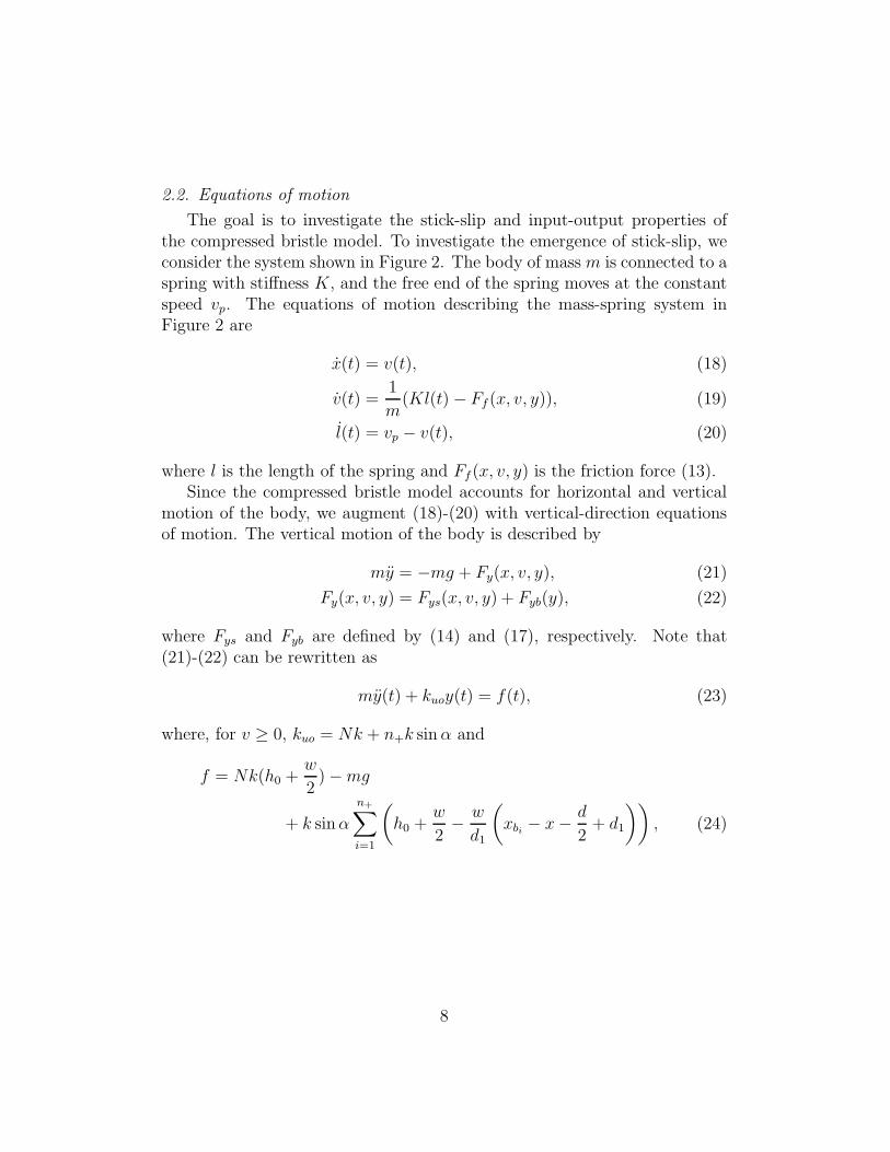
2.2. Equations of motion

The goal is to investigate the stick-slip and input-output properties ofthe compressed bristle model. To investigate the emergence of stick-slip, weconsider the system shown in Figure 2. The body of mass m is connected to aspring with stiffness K, and the free end of the spring moves at the constantspeed vp. The equations of motion describing the mass-spring system inFigure 2 are

x(t) = v(t), (18)

v(t) =1

m(Kl(t)− Ff (x, v, y)), (19)

l(t) = vp − v(t), (20)

where l is the length of the spring and Ff (x, v, y) is the friction force (13).Since the compressed bristle model accounts for horizontal and vertical

motion of the body, we augment (18)-(20) with vertical-direction equationsof motion. The vertical motion of the body is described by

my = −mg + Fy(x, v, y), (21)

Fy(x, v, y) = Fys(x, v, y) + Fyb(y), (22)

where Fys and Fyb are defined by (14) and (17), respectively. Note that(21)-(22) can be rewritten as

my(t) + kuoy(t) = f(t), (23)

where, for v ≥ 0, kuo = Nk + n+k sinα and

f = Nk(h0 +w

2)−mg

+ k sinα

n+∑

i=1

(

h0 +w

2−

w

d1

(

xbi − x−d

2+ d1

))

, (24)

8

and, for v < 0, kuo = Nk + n−k sinα and

f = Nk(h0 +w

2)−mg

+ k sinα

n−∑

i=1

(

h0 +w

2−

w

d1

(

x−d

2+ d1 − xbi

))

. (25)

Thus (21)-(22) describe an undamped oscillator.

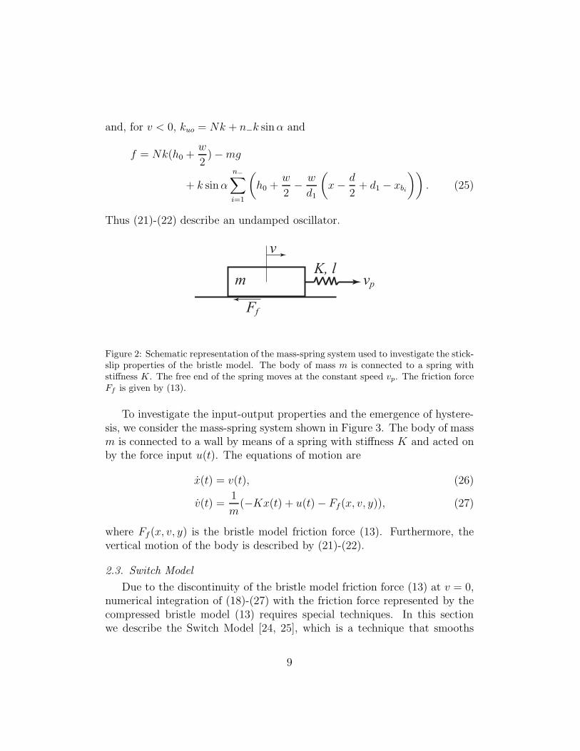
Ff

v

K, lvpm

Figure 2: Schematic representation of the mass-spring system used to investigate the stick-slip properties of the bristle model. The body of mass m is connected to a spring withstiffness K. The free end of the spring moves at the constant speed vp. The friction forceFf is given by (13).

To investigate the input-output properties and the emergence of hystere-sis, we consider the mass-spring system shown in Figure 3. The body of massm is connected to a wall by means of a spring with stiffness K and acted onby the force input u(t). The equations of motion are

x(t) = v(t), (26)

v(t) =1

m(−Kx(t) + u(t)− Ff (x, v, y)), (27)

where Ff (x, v, y) is the bristle model friction force (13). Furthermore, thevertical motion of the body is described by (21)-(22).

2.3. Switch Model

Due to the discontinuity of the bristle model friction force (13) at v = 0,numerical integration of (18)-(27) with the friction force represented by thecompressed bristle model (13) requires special techniques. In this sectionwe describe the Switch Model [24, 25], which is a technique that smooths

9

u

Ff

Km

Figure 3: Body-spring configuration used to investigate the input-output properties of thebristle model. The body of mass m is connected to the wall by a means of a spring withstiffness K and is acted on by the force input u(t). The friction force Ff is given by (13).

out the discontinuous dynamics around the discontinuity v = 0. The mod-ified equations can then be integrated using standard numerical integrationtechniques.

To begin, we rewrite the equations of motion in which the friction forceis modeled by the compressed bristle model as a differential inclusion [25].Assume that the motion of the body is described by

x = f (x), (28)

where x ∈ Rm, f : V ⊂ R

m → Rm is a piecewise continuous vector field,

and Σ4

= Rm\V is the set of points of discontinuity of f . We assume that

there exists a function g : Rm → R such that the discontinuity boundary Σis given by the roots of g, that is,

Σ = {x ∈ Rm : g(x) = 0}. (29)

We also define sets

V+4

= {x ∈ Rm : g(x) > 0}, (30)

V−

4

= {x ∈ Rm : g(x) < 0}. (31)

With these definitions, (28) can be rewritten as the differential inclusion[25, 26]

x ∈

f+(x), x ∈ V+,

αf+(x) + (1− α)f−(x), x ∈ Σ, α ∈ [0, 1],

f−(x), x ∈ V−.

(32)

10

The direction of flow given by the vector fields f+(x) and f−(x) can

lead to three types of sliding modes across Σ. If the flow is such that thesolutions of (32) are pushed to Σ from both V+ and V−, then the sliding modeis attractive. If the solutions cross Σ, then the sliding mode is transversal.Finally, if the solutions diverge from Σ, the sliding mode is repulsive [25].

The Switch Model smooths out the dynamics of the differential inclusion

(32) by constructing a stick band within the set G4

= {x : |g(x)| ≤ η},where η is a small positive constant. (Note that the term “stick band” is notrelated to stick-slip friction.) The dynamics outside of the stick band remainthe same. The dynamics inside the stick band depend on the type of slidingmode across the discontinuity boundary. If the sliding mode is attractive,that is,

nTf−(x) > 0 and nTf+(x) < 0, x ∈ Σ, (33)

where n4

= ∇g(x) is the normal to Σ, then the stick-band dynamics are givenby

x = αf+(x) + (1− α)f−(x) , x ∈ G. (34)

The value of the parameter α is chosen such that it pushes the solutions of(33) toward the middle of the stick band, that is, toward {x : g(x) = 0}.Thus, inside the stick band, g satisfies

g(x) = −τg(x), (35)

where τ > 0 is a time constant. Since

g(x) =dg(x)

dx

dx

dt= ∇gT x (36)

= nT(

αf+(x) + (1− α)f−(x)

)

, (37)

setting (35) equal to (37) and solving for α gives

α =nTf

−(x) + τ−1g(x)

nT (f−(x)− f+(x))

. (38)

11

If the sliding mode is transversal, that is,

(nTf−(x))(nTf+(x)) > 0, x ∈ Σ, (39)

then the stick-band dynamics are defined by

x =

{

f−(x), if nTf

−(x) < 0 and nTf+(x) < 0 , x ∈ G,

f+(x), if nTf

−(x) > 0 and nTf+(x) > 0 , x ∈ G.

(40)

Finally, if the sliding mode is repulsive, that is,

nTf−(x) < 0 and nTf+(x) > 0, x ∈ Σ, (41)

then the dynamics are defined by

x = f+(x) , x ∈ G. (42)

Outside of the stick band, the dynamics are defined by

x =

{

f+(x), x ∈ G+,

f−(x), x ∈ G−,

(43)

where G+4

= {x : g(x) > η} and G−

4

= {x : g(x) < η}. More details aboutthe Switch Model (33)-(43) and a pseudocode are given in [25].

2.4. Stick-slip behavior

In this section we consider the stick-slip behavior of the bristle model (13)by investigating the existence of a stable limit cycle when the bristle modelis used to represent the friction force in the system (18)-(20) shown in Figure2 with the vertical motion described by (21)-(22).

We use the Switch Model (33)-(43) to simulate the system (18)-(22) withfriction force defined by (13). The system (18)-(22) can be formulated as the

differential inclusion (32) with x =[

x v l y y]T, the set Σ defined by

the roots of the function g(x) = v, the normal to Σ defined by n4

= ∇g(x) =

12

[

0 1 0 0 0]T, and the vector fields f+(x) and f

−(x) defined as

f+(x)4

=

v1m(Kl − Ff+(x, y))

vp − v

y

−mg + Fy+(x, y)

, (44)

f−(x)

4

=

v1m(Kl − Ff−(x, y))

vp − v

y

−mg + Fy−(x, y)

, (45)

where Ff+(x, y) and Ff−(x, y) are defined by (10) and (12), respectively, and

Fy+(x, y)4

= Fys+(x, y) + Fyb(y), (46)

Fy−(x, y)4

= Fys−(x, y) + Fyb(y), (47)

where Fys+(x, y) is defined by (15) and Fys−(x, y) by (16).Figure 4(a) shows the projection of the trajectories of (44)-(45) onto the

l-v plane, obtained by using the Switch Model (33)-(43), with parametervalues m = 1 kg, w = 1 m, d = 2 m, α = 15◦, K = 5 N/m, N = 500,k = 0.01 N/m, h0 = 2.69 m, η = 10−6, and vp = 0.1 m/s. In this plane, thetrajectory converges to a stable limit cycle that includes a line segment onwhich the motion is given by v = 0 and l = vp. This segment correspondsto the “stick” phase, during which the body is stationary. The “slip” phasecorresponds to the curved part of the limit cycle for which v 6= 0. The timehistories of the spring length, velocity, height, and position of the body areshown in Figure 4(b). Note that the velocity is characterized by segments inwhich the velocity is zero and segments in which velocity quickly increases.This behavior is typical for stick-slip motion.

The time history of the friction force and plots of the friction force versusheight y and versus velocity v are shown in Figure 5. This figure also showsthe relationship between the height y and velocity v. The friction force isa decreasing function of height, which is consistent with the experimentalresults presented in [2, 4, 5] as well as the expression (13). In the bristlemodel, as the height increases, compression of the bristles from their relaxed

13

0 0.05 0.1 0.15 0.2 0.25 0.3 0.35−0.05

0

0.05

0.1

0.15

0.2

0.25

0.3

0.35

Spring Length, l [m]

Velocity, v [m/s]

stick

slip

(a)

0 10 20 300

0.1

0.2

0.3

0.4

Time, t [s]

Spr

ing

Leng

th, l

[m]

0 10 20 30−0.2

0

0.2

0.4

Time, t [s]

Vel

ocity

, v [m

/s]

0 10 20 300.8

1

1.2

1.4

1.6

Time, t [s]

Hei

ght,

y [s

]

0 10 20 30−1

0

1

2

3

Time, t [s]

Pos

ition

, x [m

]

(b)

Figure 4: The stick-slip limit cycle and time histories of the spring length l, velocity v,position x, and height y for the system (44)-(45) with Ff modeled by (13). (a) shows thelimit cycle and (b) shows the time histories of the states. The trajectories projected ontothe l-v plane form a stable limit cycle.

length h0 decreases. Thus, the friction force decreases also. Furthermore, thefriction force decreases as the velocity increases. The velocity/friction-forcecurve forms a loop, which we refer to as the dynamic Stribeck effect. Theheight versus velocity plot in Figure 5 shows that the velocity increases withheight. That is, the body moves higher as it speeds up, and it moves loweras it slows down. This is planing.

14

0 10 20 300

0.5

1

Time, t [s]

Fric

tion

For

ce, F

f [N]

0.8 1 1.2 1.4 1.60.8

1

1.2

1.4

1.6

Height, y [m]

Fric

tion

For

ce, F

f [N]

−0.1 0 0.1 0.2 0.30

0.5

1

Velocity, v [m/s]

Fric

tion

For

ce, F

f [N]

−0.2 0 0.2 0.40.8

1

1.2

1.4

1.6

Velocity, v [m/s]

Hei

ght,

y [m

]Figure 5: The friction force of the compressed bristle model. The figure shows the depen-dence of the friction force on time t, height y, and velocity v. The lower left plot showsthe dynamic Stribeck effect, while the lower right plot shows the velocity-height curve.

2.5. Physical mechanism that leads to the dynamic Stribeck effect

In the vertical direction, the system consisting of the body and the bristlesdescribed by (21)-(22) represents an undamped oscillator. Thus, if the bodyis initially not in a vertical equilibrium or if it is slightly disturbed from anequilibrium position, then it oscillates vertically whether or not it is movinghorizontally. Since the friction force (13) depends linearly on the height y

through hi(x, v, y), the vertical oscillation of the body results in oscillation ofthe magnitude of the friction force Ff defined by (13). The oscillations in Ff

are visible in Figure 5. The horizontal velocity increases with y because thefriction force Ff decreases as y increases, and thus the horizontal accelerationof the body increases. The opposite happens when y decreases.

Furthermore, as seen in Figure 5, the drop in the friction force that occurswhen a single bristle transitions from contacting the slanted surface of thebody to contacting the horizontal surface of the body is small compared tothe amplitude of oscillation of the friction force due to vertical oscillation ofthe body. As the amplitude of the vertical oscillation of the body decreases,the change in friction force due to a bristle transition from contacting theslanted surface of the body to contacting the horizontal surface of the bodybecomes the mechanism that leads to stick-slip. In comparison with thediscontinuous rotating bristle model [19, 20], the individual bristles do nothave a visible effect on the stick-slip behavior or the dynamic Stribeck effectof the compressed bristle model.

15

To demonstrate, we simulate (18)-(20) with the friction force (13). How-ever, in the vertical direction we assume that the body oscillates accordingto y(t) = A sin(ωt). We use the Switch Model (33)-(43), and reformulate(18)-(20) as a differential inclusion with f+ and f

−defined by

f+(x)4

=

v1m(Kl − Ff+(x, y))

vp − v

, (48)

f−(x)

4

=

v1m(Kl − Ff−(x, y))

vp − v

, (49)

where Ff+(x, y) is defined by (10) and Ff−(x, y) is defined by (12).The results are shown in Figure 6 for A = 0.3 m and A = 1.3 m and

for ω = 6.8 rad/s. This frequency of oscillation is approximately equal tothe natural frequency of the vertical oscillations of the body shown in Figure4(b). The parameter values used are m = 1 kg, K = 2 N/m, w = 1 m,d = 2 m, α = 15◦, N = 100, k = 0.05 N/m, and h0 = 4.46 m. Note that thedynamic Stribeck effect as well as the dependence of velocity on the height yof the body are more prominent for larger values of A. Also, once the bodybegins moving horizontally, the friction force becomes less smooth, that is,there are small drops in the friction force that correspond to the transitionof a bristle from contacting the slanted surface of the body to contacting thehorizontal surface of the body.

2.6. Hysteresis map

In this section we analyze the input-output properties of the bristle model.We consider the mass-spring configuration shown in Figure 3 and describedby (21)-(27). We use the Switch Model (33)-(43) to smooth out the discon-tinuity in the bristle model friction force (13).

The system (21)-(27) can be formulated as a differential inclusion (32)

with x =[

x v y y]T, the set Σ defined by the roots of function g(x) =

v, the normal to Σ defined by n4

= ∇g(x) =[

0 1 0 0]T, and vector

16

0 10 20 300

1

2

3

Time, t [s]

Fric

tion

For

ce, F

f [N]

1 2 3 4 50

1

2

3

Height, y [m]

Fric

tion

For

ce, F

f [N]

−0.1 0 0.1 0.2 0.30

1

2

3

Velocity, v [m/s]

Fric

tion

For

ce, F

f [N]

−0.1 0 0.1 0.2 0.31

2

3

4

5

Velocity, v [m/s]

Hei

ght,

y [m

]

A = 0.3A = 1.3

Figure 6: Simulations of (44)-(45) with the prescribed height trajectory y(t) = A sin(ωt),where A = 0.3 m and A = 1.3 m and for ω = 6.8 rad/s and Ff modeled by (13). Thedynamic Stribeck effect can be seen in the lower left plot. This effect is more pronouncedfor the vertical oscillation with the larger amplitude.

fields f+(x) and f−(x) defined as

f+(x)4

=

v1m(−Kx+ u− Ff+(x, y))

y

−mg + Fy+(x, y)

, (50)

f−(x)

4

=

v1m(−Kx+ u− Ff−(x, y))

y

−mg + Fy−(x, y)

, (51)

where Ff+(x, y) and Ff−(x, y) are defined by (10) and (12), respectively, andFy+(x, y) and Fy−(x, y) are defined by (46) and (47), respectively.

The input-output map of (50)-(51), obtained from the Switch Model (33)-(43), with parameter values m = 1 kg, K = 2 N/m, w = 1 m, d = 2 m,α = 15◦, g = 10 m/s2, N = 500, ∆ = 0.0035 m, h0 = 1.65 m, k = 0.01N/m, η = 10−6, and u(t) = 2 sin(0.01t) N is shown in Figure 7(a). Thetime histories of the states and the friction force are shown in Figure 7(b).Since the plot of the input u(t) versus position of the body x forms a loopat a low frequency of the input, the system (50)-(51) with friction forcedescribed by (13) is hysteretic [18]. During the motion, the energy is stored

17

in the bristles and dissipated by the oscillation of the bristles once the masspasses over them. The energy dissipation is manifested in the force-positionhysteresis loop, whose area 2.384 J is equal to the amount of dissipatedenergy. Note that the hysteresis map has a staircase shape typical of stick-slip motion. Furthermore the time history of the velocity shows jumps in thevelocity, which means that the body goes through periods of sticking, wherethe velocity is zero, followed by slipping, where the velocity is nonzero.

The plots in Figure 8 show the height and velocity versus the frictionforce. In accordance with [4] the magnitude of the friction force decreaseswith height. Furthermore, the magnitude of the friction force drops withan increase in velocity, and the friction force-velocity curve forms a loop asshown in Figure 8, which indicates the presence of the dynamic Stribeckeffect.

3. Simplified Bristle Model

In this section we introduce a simplified version of the bristle model,which eliminates the need for the Switch Model. The simplified bristle model(SBM) is a single-state model [3, 27–29] that captures the stick-slip propertiesand the characteristics of the friction force-height, friction force-velocity, andvelocity-height relationships of the compressed bristle model.

3.1. Single-state friction models

Single-state friction models such as the Dahl and LuGre model involvea state variable z that represents the internal friction mechanism. Thesemodels have the form

z = v

(

1− α(v, z)sign(v)z

zss(v)

)

, (52)

Ff = σ0z + σ1z + σ2v, (53)

where σ0, σ1, σ2 are positive constants, z is the internal friction state, zss(v)determines the shape of the steady-state z curve, and Ff is the friction force.The function α(v, z) determines the presence and type of elastoplastic pres-liding displacement [27, 28]. For simplicity, we set α(v, z) = 1 and rewrite

18

−2 −1.5 −1 −0.5 0 0.5 1 1.5 2−0.8

−0.6

−0.4

−0.2

0

0.2

0.4

0.6

Force Input, u [N]

Po

siti

on

, x [

m]

(a)

0 200 400 600 800−1

−0.5

0

0.5

1

Time, t [s]

Pos

ition

, x [m

]

0 200 400 600 800−0.05

0

0.05

Time, t [s]

Vel

ocity

, v [m

/s]

0 200 400 600 800−0.2

0

0.2

0.4

0.6

Time, t [s]

Hei

ght,

y [m

]

0 200 400 600 800−2

−1

0

1

2

Time, t [s]

Fric

tion

For

ce, F

f [N]

(b)

Figure 7: The input-output map and time histories of the position x, velocity v, height y,and friction force Ff of the mass-spring system shown in Figure 3 with the friction forcemodeled by (13). The input-output map is hysteretic due to the energy dissipated in orderto compress the bristle springs. The energy dissipated is equal to the area of the hysteresismap.

(52)-(53) as

z = v −|v|

zss(v)z, (54)

Ff = σ0z + σ1z + σ2v. (55)

19

−0.2 0 0.2 0.4 0.6−2

−1

0

1

2

Height, y [m]

Fric

tion

forc

e, F

f [N]

−0.04 −0.02 0 0.02 0.04−2

−1

0

1

2

Velocity, v [m/s]

Fric

tion

forc

e, F

f [N]

Figure 8: Dependence of friction force on height and velocity. The magnitude of thefriction force decreases with increasing height and velocity. The drop in friction force withincreased velocity is the Stribeck effect.

Setting zss(v) to be

zss(v) =1

σ0

(

Fc + (Fs − Fc)e−(v/vs)2

)

, (56)

where Fc, Fs, and vs are constants, yields the LuGre model [10, 11], whichexhibits stick-slip, hysteresis, and the Stribeck effect.

In steady-state motion, z = 0, and thus z = sign(v)zss(v). Furthermore,if σ1 = σ2 = 0, then

Ff = σ0z = sign(v)σ0zss(v). (57)

3.2. Mean friction force

The goal in formulating the SBM is to capture the characteristics of thefriction force-height, friction force-velocity, and velocity-height relationshipsof the bristle model, while redefining the bristle model equations as a con-tinuous model. As shown in Figure 5, the friction force-velocity and height-velocity curves form loops. To model these loops, we fit a function to themean values of each loop and then reformulate the compressed bristle modelequations in the form of a single-state friction model.

First, we find the mean value of the friction force as a function of heighty. For all v ≥ 0, the bristle height hi+(x, y) is calculated from (2), and theith bristle contributes to the friction force if xbi ∈ Xb+(x) defined by (7), that

20

is,

x+d

2− d1 ≤ xbi ≤ x+

d

2. (58)

Thus, over all relevant values of xbi , hi+(x, y) takes on the maximum andminimum values

hi+,max(x, y) = y −w

2+

w

d2

(

x+d

2− d1 −

(

x+d

2− d1

))

= y −w

2, (59)

hi−,min(x, y) = y −w

2+

w

d2

(

x+d

2−

(

x+d

2− d1

))

= y +w

2. (60)

Similarly, for all v < 0, the bristle height hi−(x) is found from (3), and theith bristle contributes to the friction force if xbi ∈ Xb−(x) defined by (8), thatis,

x−d

2≤ xbi ≤ x−

d

2+ d1. (61)

Thus, over all relevant values of xbi , hi−(x, y) takes on the maximum andminimum values

hi−,max(x, y) = y −w

2+

w

d

(

x−d

2+ d1 −

(

x−d

2+ d1

))

= y −w

2, (62)

hi−,min(x, y) = y −w

2+

w

d

(

x−d

2+ d1 −

(

x−d

2

))

= y +w

2. (63)

Thus, for all v ∈ R, the mean value of the ith bristle height hi(x, v, y) is

hi(y) =1

2

(

y +w

2+ y −

w

2

)

= y, (64)

and the mean value of the friction force is

Ff(x, v, y) =

{

k cos(α)∑n+

i=1 h0 − hi = n+k cos(α)(h0 − hi), if v ≥ 0,

−k cos(α)∑n−

i=1 h0 − hi = −n−k cos(α)(h0 − hi), if v < 0.

(65)

21

where h0 − hi denotes the mean value of h0 − hi. To find h0 − hi, we use

h0 − hi =

∑ni=1(h0 − hi)

n= h0 −

∑ni=1 hi

n= h0 − hi = h0 − y, (66)

so that

Ff (y, v) = sign(v)kn cos(α)(h0 − y) = sign(v)k(h0 − y), (67)

where k = kn cos(α) and we assume that n+ = n− = n. Equation (67)describes the friction force as a function of height.

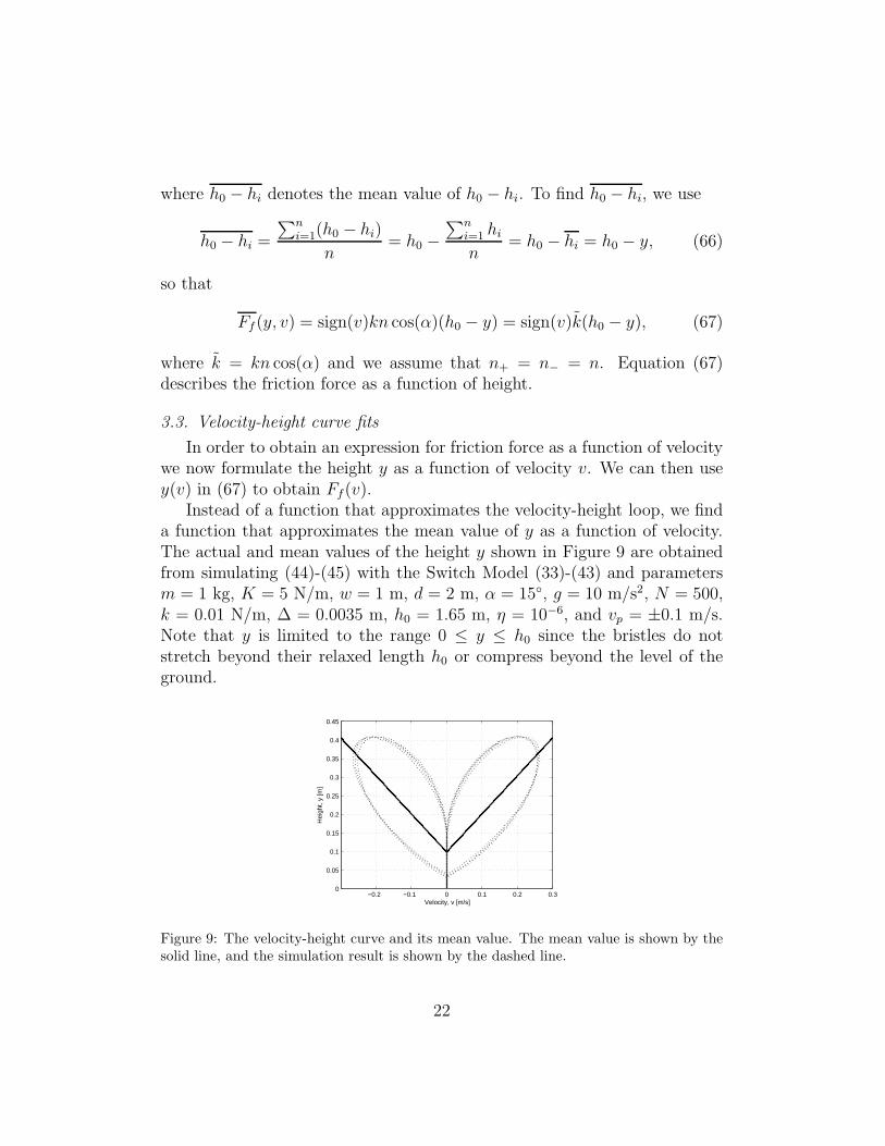
3.3. Velocity-height curve fits

In order to obtain an expression for friction force as a function of velocitywe now formulate the height y as a function of velocity v. We can then usey(v) in (67) to obtain Ff(v).

Instead of a function that approximates the velocity-height loop, we finda function that approximates the mean value of y as a function of velocity.The actual and mean values of the height y shown in Figure 9 are obtainedfrom simulating (44)-(45) with the Switch Model (33)-(43) and parametersm = 1 kg, K = 5 N/m, w = 1 m, d = 2 m, α = 15◦, g = 10 m/s2, N = 500,k = 0.01 N/m, ∆ = 0.0035 m, h0 = 1.65 m, η = 10−6, and vp = ±0.1 m/s.Note that y is limited to the range 0 ≤ y ≤ h0 since the bristles do notstretch beyond their relaxed length h0 or compress beyond the level of theground.

−0.2 −0.1 0 0.1 0.2 0.30

0.05

0.1

0.15

0.2

0.25

0.3

0.35

0.4

0.45

Velocity, v [m/s]

Hei

ght,

y [m

]

Figure 9: The velocity-height curve and its mean value. The mean value is shown by thesolid line, and the simulation result is shown by the dashed line.

22

To approximate the mean value of the velocity-height curve, we choosetwo different functions, namely, hyperbolic secant and exponential. The hy-perbolic secant expression is

y(v) = y1 − y2sech

(

v

vs

)

, (68)

where y1 and y2 determine the maximum and minimum values of y and vs isthe velocity at which the height increases from y1 to y2. If y(v) is defined by(68), then the approximation of the mean friction force is

Ff(v) = sign(v)k

(

h0 − y1 + y2sech

(

v

vs

))

. (69)

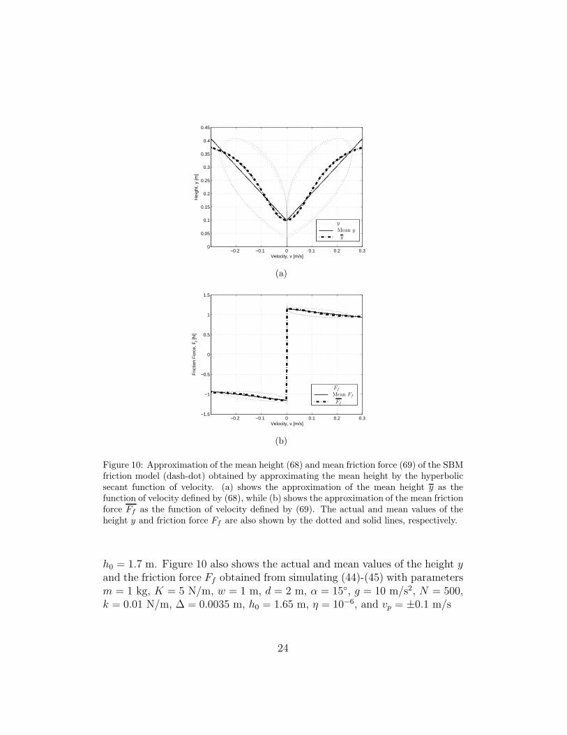
Figure 10(a) shows the approximation of the mean height y as the functionof velocity defined by (68), while Figure 10(b) shows the approximation ofthe mean friction force Ff as the function of velocity defined by (69) withthe parameter values y1 = 0.4 m, y2 = 0.3 m, vs =

0.62π

m/s, k = 0.75 N/m,and h0 = 1.64 m. Figure 10 also shows the actual and mean values of theheight y and the friction force Ff obtained from simulating (44)-(45) withparameters m = 1 kg, K = 5 N/m, w = 1 m, d = 2 m, α = 15◦, g = 10m/s2, N = 500, k = 0.01 N/m, ∆ = 0.0035 m, h0 = 1.65 m, η = 10−6, andvp = ±0.1 m/s

Alternatively, we can approximate the mean height by the exponentialfunction of velocity

y(v) = y1 − y2e−(v/vs)2 , (70)

where y1 and y2 are the maximum and minimum values of mean height,respectively, and vs is the velocity at which the mean height increases fromy2 to y1. If y is defined by (70), then the approximation of the mean frictionforce is

Ff(v) = sign(v)k(

h0 − y1 + y2e−(v/vs)2

)

. (71)

Figure 11(a) shows the approximation of the mean height y as the functionof velocity defined by (70), while Figure 11(b) shows the approximation ofthe mean friction force Ff as the function of velocity defined by (71) withparameters y1 = 0.4 m, y2 = 0.3 m, vs = 0.1 m/s, k = 0.75 N/m, and

23

−0.2 −0.1 0 0.1 0.2 0.30

0.05

0.1

0.15

0.2

0.25

0.3

0.35

0.4

0.45

Velocity, v [m/s]

Hei

ght,

y [m

]

y

Mean y

y

(a)

−0.2 −0.1 0 0.1 0.2 0.3−1.5

−1

−0.5

0

0.5

1

1.5

Velocity, v [m/s]

Fric

tion

For

ce, F

f [N]

Ff

Mean Ff

Ff

(b)

Figure 10: Approximation of the mean height (68) and mean friction force (69) of the SBMfriction model (dash-dot) obtained by approximating the mean height by the hyperbolicsecant function of velocity. (a) shows the approximation of the mean height y as thefunction of velocity defined by (68), while (b) shows the approximation of the mean frictionforce Ff as the function of velocity defined by (69). The actual and mean values of theheight y and friction force Ff are also shown by the dotted and solid lines, respectively.

h0 = 1.7 m. Figure 10 also shows the actual and mean values of the height yand the friction force Ff obtained from simulating (44)-(45) with parametersm = 1 kg, K = 5 N/m, w = 1 m, d = 2 m, α = 15◦, g = 10 m/s2, N = 500,k = 0.01 N/m, ∆ = 0.0035 m, h0 = 1.65 m, η = 10−6, and vp = ±0.1 m/s

24

−0.2 −0.1 0 0.1 0.2 0.30

0.05

0.1

0.15

0.2

0.25

0.3

0.35

0.4

0.45

Velocity, v [m/s]

Hei

ght,

y [m

]

y

Mean y

y

(a)

−0.2 −0.1 0 0.1 0.2 0.3−1.5

−1

−0.5

0

0.5

1

1.5

Velocity, v [m/s]

Fric

tion

For

ce, F

f [N]

Ff

Mean Ff

Ff

(b)

Figure 11: Approximation of the mean height (70) and mean friction force (71) of the SBMfriction model (dash-dot) obtained by approximating the mean height by an exponentialfunction of velocity with parameters y1 = 1 m, y2 = 0.5 m, vs = 0.1 m/s, k = 1 N/m, andh0 = 2 m. (a) shows the approximation of the mean height y as the function of velocitydefined by (70), (b) shows the approximation of the mean friction force Ff as the functionof velocity defined by (71). The actual and mean values of the height y and friction forceFf are also shown by the dotted and solid lines, respectively.

Combining (57) and (69) yields

zss(v) =k

σ0

(

h0 − y1 + y2sech

(

v

vs

))

, (72)

25

and the single-state friction model

z = v − σ0|v|

k(

h0 − h1 + h2sech(

vvs

))z, (73)

Ff = σ0z. (74)

Furthermore, combining (57) and (71) gives the alternative expression

zss =k

σ0

(

h0 − y1 + y2e−(v/vs)2

)

, (75)

and the alternative single-state friction model

z = v − σ0|v|

k (h0 − y1 + y2e−(v/vs)2)z, (76)

Ff = σ0z. (77)

The equations (76)-(77) are identical to the LuGre equations (54)-(56) withσ1 = σ2 = 0, k(h0 − y1) = Fc, and ky2 = Fs − Fc. In order to furtherdemonstrate the similarity of the LuGre model and the simplified bristlemodel, we simulate the systems of equations (18)-(20) and (26)-(27) withthe friction force (76)-(77). The output of the system (18)-(20) with thefriction force (76)-(77) and input velocity vp = 0.1 m/s is shown in Figure12(a). The parameter values are m = 1 kg, K = 1 N/m, y1 = 1 m, y2 = 0.5m, vs = 0.1 m/s, k = 1 N/m, σ = 105, and h0 = 2 m. The results ofsimulating (26)-(27) with the friction force (76)-(77) and input defined byu(t) = 5 sin(0.01t) N, are shown in Figure 12(b). The stick-slip behavioris visible in both simulations, and the system is hysteretic as shown by thehysteretic input-output map.

4. Conclusions

In this paper we developed the compressed bristle model, an asperity-based friction model in which the friction force arises through the frictionlessand lossless interaction of a body with an endless row of bristles that representthe microscopic roughness of the contacting surfaces. The bristles consist ofa frictionless roller attached to the ground through a spring. The body isallowed to move horizontally and vertically over the bristles, which are com-

26

0 0.2 0.4 0.6 0.8 1 1.2 1.4 1.6−0.1

0

0.1

0.2

0.3

0.4

0.5

0.6

0.7

Spring Length, l [m]

Vel

ocity

, v [m

/s]

(a)

−5 0 5−4

−3

−2

−1

0

1

2

3

4

Force Input, u [N]

Po

siti

on

, x [

m]

(b)

Figure 12: The stick-slip limit cycle of (18)-(20) and the hysteresis map of (26)-(27) withfriction force modeled by (76)-(77). The stick-slip limit cycle in the l-v plane is shown in(a). (b) shows the hysteresis map with staircase shape typical of stick-slip motion.

pressed and thus apply a reaction force at the point of contact. The frictionforce is the sum of all horizontal components of the contact forces between allof the bristles and the body. As the body passes over the compressed bristles,they are suddenly released, and the energy stored in each spring is dissipatedby viscous dashpot regardless of how slowly the body moves. Thus, energyis dissipated in the limit of DC operation and the system is hysteretic.

In the vertical direction, the body and the bristles form an undampedoscillator. The body oscillates vertically regardless of whether it is movinghorizontally or not. During the vertical oscillations, as the body rises, thefriction force decreases, and the body speeds up. This mechanism gives riseto the dynamic Stribeck effect, which refers to the fact that the frictionforce-velocity curve forms a loop.

Furthermore, we showed that the compressed bristle model exhibits stick-slip friction and that the bristle model equations can be simplified to givea single-state friction model. The simplified bristle model (SBM) retainsthe stick-slip and hysteresis properties of the original model. The internalfriction state of the SBM can be interpreted as the average deflection of thebristles from their relaxed length. The simplified bristle model is equivalentto the LuGre model.

27

5. Acknowledgments

This research was made with Government support under and awarded byDoD, Air Force Office of Scientific Research, National Defense Science andEngineering Graduate (NDSEG) Fellowship, 32 CFR 168a and NSF grant0758363.

References

[1] B. Armstrong-Helouvry, Control of Machines with Friction, Kluwer,Boston, MA, 1991.

[2] B. Armstrong-Helouvry, P. Dupont, C. Canudas de Wit, A survey ofmodels, analysis tools and compensation methods for the control of ma-chines with friction, Automatica 30 (1994) 1083–1138.

[3] J. J. Choi, S. I. Han, J. S. Kim, Development of a novel dynamic frictionmodel and precise tracking control using adaptive back-stepping slidingmode controller, Mechatronics 16 (2006) 97–104.

[4] D. M. Tolstoi, Significance of the normal degree of freedom and naturalnormal vibrations in contact friction, Wear 10 (1967) 199–213.

[5] T. Sakamoto, Normal displacement and dynamic friction characteristicsin a stick-slip process, Tribology International 20 (1987) 25–31.

[6] J. A. C. Martins, J. T. Oden, F. M. F. Simoes, Recent advances inengineering science: A study of static and kinetic friction, Int. J. Engng.Sci. 28 (1990) 29–92.

[7] C. Canudas de Wit, H. Olsson, K. J. Astrom, P. Lischinsky, A newmodel for control of systems with friction, IEEE Trans. Autom. Contr.40 (1995) 419–425.

[8] H. Olsson, K. J. Astrom, C. Canudas de Wit, M. Gafvert, P. Lischinsky,Friction models and friction compensation, European Journal of Control4 (1998) 176–195.

[9] N. Barabanov, R. Ortega, Necessary and sufficient conditions for passiv-ity of the LuGre friction model, IEEE Trans. Autom. Contr. 45 (2000)675–686.

28

[10] F. Avanzini, S. Serafin, D. Rocchesso, Modeling interaction betweenrubbed dry surfaces using an elasto-plastic friction model, in: Proc.5th Int. Conference on Digital Audio Effects, Hamburg, Germany, pp.111–116.

[11] K. J. Astrom, C. Canudas de Wit, Revisiting the LuGre friction model,IEEE Control Systems Magazine 28 (2008) 101–114.

[12] A. K. Padthe, N. A. Chaturvedi, D. S. Bernstein, S. P. Bhat, A. M.Waas, Feedback stabilization of snap-through buckling in a preloadedtwo-bar linkage with hysteresis, Int. J. Non-Linear Mech. 43 (2008)277–291.

[13] A. K. Padthe, B. Drincic, J. Oh, D. D. Rizos, S. D. Fassois, D. S.Bernstein, Duhemmodeling of friction-induced hysteresis: Experimentaldetermination of gearbox stiction, IEEE Contr. Sys. Mag. 28 (2008) 90–107.

[14] D. A. Haessig, B. Friedland, On the modeling and simulation of friction,ASME J. Dyn. Sys. Meas. Contr. 113 (1991) 354–361.

[15] N. E. Dowling, Mechanical Behavior of Materials: Engineering Methodsfor Deformation, Fracture, and Fatigue, Prentice Hall, Englewood Cliffs,NJ, 1993.

[16] F. Al-Bender, V. Lampert, J. Swevers, A novel generic model at asperitylevel for dry friction force dynamics, Tribology Letters 16 (2004) 81–93.

[17] F. Al-Bender, J. Swevers, Characterization of friction force dynamics:Behavior and modeling on micro and macro scales, IEEE Contr. Sys.Mag. 28 (2008) 82–91.

[18] J. Oh, D. S. Bernstein, Semilinear Duhem model for rate-independentand rate-dependent hysteresis, IEEE Trans. Autom. Contr. 50 (2005)631–645.

[19] B. Drincic, D. S. Bernstein, A sudden-release bristle model that exhibitshysteresis and stick-slip friction, in: Proc. Amer. Contr. Conf., SanFrancisco, CA, pp. 2456–2461.

29

[20] B. Drincic, D. S. Bernstein, A frictionless bristle-based friction modelthat exhibits hysteresis and stick-slip behavior, J. Sound and Vibration(2012). Submitted.

[21] W. B. Horne, R. C. Dreher, Phenomena of Pneumatic Tire Hydroplan-ing, Technical Note TN D-2056, NASA, 1963.

[22] P. Andren, A. Jolkin, Elastohydrodynamic aspects on thetyre-pavement contact at aquaplaning, VTI rapport 483A,Swedish National Road and Transport Research Institute, 2003.Http://www.mobilidades.org/arquivo/aquaplanning.pdf.

[23] A. J. Tuononen, M. J. Matilainen, Real-time estimation of aquaplaningwith an optical tyre sensor, Institution of Mechanical Engineers, PartD: J. Automobile Engineering 223 (2009) 1263–1272.

[24] R. I. Leine, D. H. V. Campen, A. De Kraker, L. Van Den Steen, Stick-slip vibrations induced by alternate friction models, Nonlinear Dynamics16 (1998) 41–45.

[25] R. I. Leine, H. Nijmeijer, Dynamics and Bifurcations of Non-smoothMechanical Systems, Springer, Berlin, 2004.

[26] A. F. Filippov, Differential Equations with Discontinuous RighthandSides, Kluwer Academic Publishers, Dordrecht, The Netherlands, 1988.

[27] P. Dupont, B. Armstrong, V. Hayward, Elasto-plastic friction model:Contact compliance and stiction, in: Proc. Amer. Contr. Conf., Chicago,IL, pp. 1072–1077.

[28] P. Dupont, V. Hayward, B. Armstrong, F. Altpeter, Single state elasto-plastic friction models, IEEE Trans. Autom. Contr. 47 (2002) 787–792.

[29] B. S. R. Armstrong, Q. Chen, The z-properties chart: Visualizing thepresliding behavior of state-variable friction models, IEEE Control Sys-tems Magazine 28 (2008) 79–89.

30