A DYNAMIC

QUANTITATIVE

MACROECONOMIC

MODEL OF BANK RUNS

Working Papers 2014

Elena Mattana | Ettore Panetti

13

A DYNAMIC

QUANTITATIVE

MACROECONOMIC

MODEL OF BANK RUNS

Working Papers 2014

Elena Mattana | Ettore Panetti

Lisbon, 2014 • www.bportugal.pt

13

October 2014The analyses, opinions and fi ndings of these papers represent the views of the authors, they are not necessarily those of the Banco de Portugal or the Eurosystem

Please address correspondence toBanco de Portugal, Economics and Research Department Av. Almirante Reis 71, 1150-012 Lisboa, PortugalT +351 213 130 000 | estudos@bportugal.pt

WORKING PAPERS | Lisbon 2014 • Banco de Portugal Av. Almirante Reis, 71 | 1150-012 Lisboa • www.bportugal.pt •

Edition Economics and Research Department • ISBN 978-989-678-299-3 (online) • ISSN 2182-0422 (online)

A Dynamic Quantitative Macroeconomic Model of Bank Runs∗

Elena Mattana† Ettore Panetti‡

First draft: May 2013

This draft: September 2014

Abstract

We study the macroeconomic effects of bank runs in a neoclassical growth model with

a fully microfounded banking system. In every period, the banks provide insurance against

idiosyncratic liquidity shocks, but the possibility of sunspot-driven bank runs distorts the

equilibrium allocation. In the quantitative exercise, we find that the banks, for low values

of the probability of the sunspot, choose a contract that is not run-proof, and satisfy an

“equal service constraint” if the run is realized. In equilibrium, a shock to the probability

of a bank run leads to a drop in GDP of between 0.001 and 5.6 percentage points.

Keywords: financial intermediation, bank runs, welfare costs, calibration

JEL Classification: E21, E44, G01, G20

∗We would like to thank Franklin Allen, Luca Deidda, Martin Eichenbaum, Huberto Ennis, Pedro Teles,and the seminar participants at the Stockholm School of Economics, SUDSWEc 2013, XXII MBF Conference,Universidade Católica Portuguesa, Banco de Portugal, International Economic Association 2014 World Con-ference, and the V IIBEO Workshop for their valuable comments. Financial support by FCT (Fundação paraa Ciência e a Tecnologia) Portugal is gratefully acknowledged. This article is part of the Strategic Project(Pest-OE/EGE/UI0436/2014).

†Université Catholique de Louvain-CORE, Voie du Roman Pays 34, L1.03.01, B-1348 Louvain-la-Neuve,Belgium. Email: elena.mattana@uclouvain.be

‡Economics and Research Department, Banco de Portugal, Avenida Almirante Reis 71, 1150-012 Lisboa,Portugal, and CRENoS-University of Sassari and UECE. Email: ettore.panetti@bportugal.pt

1

1 Introduction

What are the macroeconomic effects of bank runs, and how big are they? The interest in

this question arises from the observation that bank runs are not a phenomenon of the past:

in fact, they may occur whenever long-term illiquid assets are financed by short-term liquid

liabilities, and the providers of short-term funds lose confidence in the borrower’s ability to

repay, or are afraid that other lenders are losing their confidence. In that sense, there exists

a wide consensus that U.S. money market funds have experienced a run-like episode after

the bankruptcy of Lehman Brothers in 20081 and, more generally, that the financial crisis of

2007-2009 can be interpreted as a systemic run of financial intermediaries on other financial

intermediaries, that provided banking services without being regulated as actual banks.2 The

empirical literature showed how big the costs of this crisis were, with a drop in GDP of around

4.8 percentage points, followed by a recovery of around 6 years (Reinhart and Rogoff, 2014).

However, these numbers do not allow us to isolate the importance of the financial system to

explain the behavior of the real economy, and this is the reason why we need a formal theory

of systemic bank runs. The literature on the economics of banking has extensively analyzed

these issues, but mainly in static partial-equilibrium settings, that are not suitable for any

formal quantitative analysis. Thus, in the present work, we overcome the limitations of both

the empirical and the theoretical literature, and study the macroeconomic effects of systemic

bank runs in a dynamic quantitative model with a fully microfounded banking system.

Our model is based on three building blocks, all considered standard workhorses in their

own field. The first one is the neoclassical growth model: an infinite horizon, general equi-

librium, dynamic model populated by households and firms. As generally known, this model

lacks a proper role for a banking system, as the households provide capital to the firms without

any intermediation. This leads to our second building block: the theory of banking proposed

by Diamond and Dybvig (1983). In this environment, banks provide insurance to their depos-

itors against the realization of an idiosyncratic preference shock, that makes them willing to

consume before the maturity of their investment. We choose this environment for two reasons:

first, because it provides a rationale for the existence of the banking system, as a mechanism

to decentralize the efficient provision of insurance against idiosyncratic risk; second, because

it also provides a formal characterization of bank runs. As a consequence, our third building

block is the seminal paper by Cooper and Ross (1998) – and its refinements by Ennis and

Keister (2006) – where bank runs are modeled as self-fulfilling crises, during which all depos-

itors close down their accounts, because they expect everybody else to do the same, forcing

1In just two days, from September 15 to September 17, their total retail funds dropped by more than 4.5percentage points.

2In a recent op-ed on the New York Times (March 24, 2012), Tyler Cowen states that “[...] the single mostimportant development to emerge from America’s financial crisis [is the fact that] the age of the bank run hasreturned”. See Gorton and Metrick (2012) for a further analysis of this argument.

2

the banks to go bankrupt.3

More formally, our economy is populated by a continuum of infinitely-lived identical agents

who, at each point in time, are hit by an idiosyncratic private preference shock, that makes

them willing to consume either in an intermediate period, that we call “night”, or when pro-

duction takes place, in the “morning”. To hedge against these shocks, the agents form financial

coalitions – or, more commonly, “banks” – that operate in a competitive environment, and

allow them to pool the idiosyncratic risk among themselves: the agents make a deposit, and

the banks offer them a contract, stating how much they can withdraw each morning and each

night. The banks, in turn, finance the contract by investing in liquidity, that they store for the

night withdrawals, and in credit, that they provide to the production sector. In this environ-

ment, the banks, in equilibrium, offer a contract providing perfect intratemporal risk sharing,

i.e. they equalize morning and night consumption in every period, and choose a portfolio of

liquidity and credit satisfying an Euler equation, i.e. such that the marginal rate of substitu-

tion between consumption in the night of date t and in the morning of date t+ 1 is equal to

the marginal rate of transformation of the production technology.

We extend this environment with the introduction of bank runs. To this end, we show

that this economy also exhibits an equilibrium where all agents, regardless of the realization

of their preference shocks, withdraw at night, and that this equilibrium exists if the agents

know that the banks do not hold a sufficient amount of liquidity to honor the contract with all

of them. Whenever a run equilibrium and a no-run equilibrium coexist, the agents coordinate

over which one to select in accordance with the realization of a “sunspot”, i.e. an extrinsic event

happening with some given probability. This is an assumption that, at the cost of introducing

an exogenous parameter completely uncorrelated with any fundamental of the economy, allows

us to model bank runs as self-fulfilling prophecies. Arguably, this is an important point, as

many bank runs in the past – and, as we mentioned above, also in the recent financial crisis

– arose as a consequence of a coordination failure that led to a generalized panic.4

The banks, in turn, take into account the sunspot selection mechanism, and choose between

a “run-proof” contract, according to which they hold a sufficient amount of liquidity to pay

the night withdrawals of every agent even in the case of a run, and a contract that allows the

3Our focus is on one specific role (which we believe is key) played by the banking system in the real economy:the management of risk, to hedge against idiosyncratic uncertainty. In this sense, here we do not consider thebanks as monitors of investments or producers of information, as in Holmstrom and Tirole (1998) and Diamondand Rajan (2001). Similarly, in modeling financial crises as bank runs, we do not take into account crises arisingfrom shocks to the fundamentals of the economy, like in Allen and Gale (2004).

4An alternative to the equilibrium-selection mechanism based on sunspots would be a dynamic version ofthe “global game” approach of Carlsson and van Damme (1993), according to which the agents receive a noisysignal about the state of the economy, and run if the signal is lower than an endogenous threshold. Goldsteinand Pauzner (2005) successfully apply this approach to a static Diamond-Dybvig model, to guarantee theuniqueness of its equilibrium. However, Angeletos et al. (2007) show that a dynamic global game would exhibita unique equilibrium only if the agents do not learn from their signals: in fact, a global game with learningwould still exhibit arbitrarily many equilibria, under the very same conditions that guarantee the uniquenessof the equilibrium in a static environment.

3

possibility of runs. In this second case, the banks also choose how to serve their depositors.

In particular, we distinguish between two protocols: one is the “sequential service constraint”

(Wallace, 1988), according to which the banks pay the depositors on a first-come-first-served

basis, until the resources are completely exhausted; the other is, instead, the “equal service

constraint” (Allen and Gale, 1998), according to which all depositors who participate in the

run receive the same share of the available resources. We choose to analyze both cases because

there is evidence of both behaviors in the real world: while the sequential service constraint

is generally introduced to model the fact that withdrawals happens sequentially, the equal

service constraint takes into account that, at a run, the agents try to withdraw all at the same

time, in which case they are paid pro-rata.5

We characterize the run-proof equilibrium and the run equilibria, both with sequential

service and equal service. In the run-proof equilibrium, the banks, in order to be able to

serve all depositors, react to a positive probability of a run by lowering the amount of night

consumption offered in the contract and by increasing their holding of liquidity, that they

partially roll over to the following period. Thus, a positive probability of a run gives rise to a

credit tightening, with a corresponding drop in GDP, followed by a recovery.

In the run equilibrium with sequential service, instead, the banks react to a positive proba-

bility of a run by increasing night consumption and, as a consequence, the amount of liquidity

in portfolio: this happens because, at a run, the objective of increasing the welfare of the depos-

itors, that would motivate the banks to increase night consumption, dominates the objective

of serving the highest possible fraction of them, that would instead motivate them to lower

night consumption. Thus, a run gives rise to a credit tightening, that leads, in turn, to a drop

in GDP. Importantly, the equilibrium credit tightening is not contingent on the ex-post real-

ization of a run. Thus, it is just the possibility of a run that pushes the banks to tighten credit.

This also means that the fraction of depositors served when the run equilibrium is selected is

equal to the fraction served when the no-run equilibrium is selected. Therefore, the ex-post

realization of a run does not affect the amount of credit provided to the production sector,

but only the fraction of depositors that are not served and consume zero, with a substantial

effect on total welfare. Finally, in the run equilibrium with equal service, the banks, at least

qualitatively, behave in a similar way as in the case with sequential service: they react to a

positive probability of a run by increasing night consumption and tightening credit. However,

there is a key difference: the equal service constraint forces the banks to serve all depositors

equally in the case of a run. This means that, contrary to what happens in the equilibrium

with sequential service, with equal service every agent consumes, even in the case of a run.

However, in order to finance such an arrangement, the banks are forced to hold, and partially

roll over to the following period, a positive amount of liquidity.

We assume that the banks choose between the three equilibria following an ex-ante welfare

5Gaytan and Ranciere (2006) mention that this was the way in which the Argentinian banks, for example,paid their depositors during the run of 2002.

4

criterion, but, as we cannot derive a closed-form solution for the expected welfare, we rely on

a numerical analysis to characterize the complete equilibrium. We assume that the economy

starts in the steady state of the no-run equilibrium (where runs are ruled out by assumption),

and is hit by a one-period shock: the probability of the realization of the sunspot spikes to

a positive number, and then goes back to zero. Then, we calculate the welfare difference (in

consumption equivalents) between our two banking equilibria and the no-run equilibrium, and

pick the one with the lowest value. To this end, we calibrate the parameters of the model to

the U.S. economy. This is an important and interesting task per se, since, to the best of our

knowledge, we are the first ones to calibrate the probability of the idiosyncratic shock of a

Diamond-Dybvig economy using the U.S. financial accounts.

With these numbers in hand, we quantitatively evaluate how a run affects the real econ-

omy in the three banking equilibria. The welfare costs of a run are always increasing in the

probability of the realization of the sunspot, as the larger the probability of a run is, the more

the banks distort the intertemporal allocation of capital. Moreover, the welfare costs of the

equilibrium with sequential service are always higher than those of the equilibrium with equal

service, and lower than those of the run-proof equilibrium only for extremely low values of the

probability of the realization of the sunspot. Hence, the banks will always prefer equal service

over sequential service. These results are based on two features of the equilibrium with se-

quential service: first, when the economy is hit by a shock to the probability of the realization

of the sunspot, a non-negligible fraction of agents consume zero, and have zero utility; second,

although the equilibrium credit tightening and the corresponding drop in GDP is lower in this

case than in the other two, the transition back to the steady state is slower, because in the

run-proof equilibrium, as well as in the equilibrium with equal service, the liquidity in excess

is rolled over, and allows a faster recovery.

When comparing the equilibrium with equal service to the run-proof equilibrium, we find

that the second is preferred to the first only when the shock to the probability of the realization

of the sunspot is above 5 per cent. Quantitatively, the equilibrium relative welfare costs of a

positive probability of a run, depending on the magnitude of the shock, are between 0.0006

and 0.1744 percentage points, and are increasing in the degree of relative risk aversion. This

happens because the higher the relative risk aversion is, the more the banks are willing to

distort the allocation of resources, and smooth the ex-post consumption profiles of the agents

between a realized and an unrealized run. Finally, a positive shock to the probability of the

realization of the sunspot leads to a drop in GDP of between 0.0011 and 5.64 percentage

points. Again, this effect is increasing in the degree of relative risk aversion of the agents.

The rest of the paper is organized as follows: in section 2, we relate our work to the existing

literature; in section 3, we define the environment, and characterize, as a benchmark, the no-

run banking equilibrium; in section 4, we introduce bank runs, and characterize the three

equilibria; in section 5, we calibrate the model to the U.S. economy, and report the results of

our quantitative exercises; finally, we conclude in section 6.

5

2 Related Literature

In the last years, macroeconomics has shifted its attention to study the role of financial frictions

as amplifiers of shocks to the real economy. In that respect, many economists are extending

their agendas to introduce some microfoundations for the financial system in otherwise stan-

dard macroeconomic models, that could be used for policy analysis. Gertler and Karadi (2011)

and Gertler and Kiyotaki (2013) are two notable examples of this line of research, where the

banks operate as intermediaries between the households (the lenders of capital) and the firms

(the borrowers of capital) and suffer from some kind of moral hazard that gives space to the

intervention of the central bank. We see our contribution as a further extension of this class of

models to formally assess the role of the financial system in a fully microfounded environment.

Starting from the seminal work of Diamond and Dybvig (1983), a series of papers provides

the microfoundations for the process of financial intermediation, based on the ability of the

intermediaries (i.e., the banks) to pool risk and offer the efficient level of insurance against

idiosyncratic shocks. However, already in their original contribution, Diamond and Dybvig

notice that this environment exhibits a multiplicity of equilibria, i.e. that there also exists a

bank-run equilibrium, in which every depositor withdraws from her account because she ex-

pects everybody else to do the same. Cooper and Ross (1998), in the same static environment,

offer a more sophisticated characterization of the run equilibrium, and show how the banks

change their portfolio allocation in reaction to the possibility of a run.

The Diamond-Dybvig model has been extensively used in dynamic environments. Ben-

civenga and Smith (1991) develop a growth model with a banking system and overlapping

generations of two-period lived depositors, that has been the base for further analysis of the

provision of intertemporal risk sharing (Qi, 1994; Allen and Gale, 1997). Ennis and Keister

(2003) and Gaytan and Ranciere (2006) provide two recent examples of models where financial

crises, in the form of bank runs, affect the intertemporal allocation of resources and harm long-

run growth. With respect to these, our work provides some similar theoretical results, but in a

representative-agent setting, that we choose for two reasons: first, because, in a dynamic OLG

model, the banks provide insurance against the risk of consuming when young versus when

old, while we believe that their activity is more targeted towards short-term shocks; second,

because, as in Ennis and Keister (2003), we cannot get to a closed-form characterization of

the equilibrium allocation. However, instead of providing a numerical solution with some a

priori parameters, we prefer a formal calibration, that the representative-agent structure of

the model makes possible.

6

3 A Dynamic Model of Banks

3.1 Environment

Time is infinite and discrete, and every period is divided into two sub-periods, that we label

1 and 2, and call for simplicity “day” and “night”. The economy is populated by a unitary

continuum of infinitely-lived agents, who are endowed with one unit of time, and want to

maximize the present discounted value of an infinite stream of utility:

W = E∞∑

t=0

βtU(c2t, c1t+1, θt), (1)

where β is a discount factor, and is smaller than 1.

All agents in the economy are affected, at every point in time, by some idiosyncratic

uncertainty, that hits them in the form of a preference shock. Being ex-ante equal, every

agent draws a type θt ∈ {0, 1}, where 0 < π < 1 is the probability of being of type 1, and

1 − π is the probability of being of type 0. The preference shocks are private information,

and are independent and identically distributed across the agents. Therefore, by the law of

large numbers, the cross-sectional distribution of the types is equivalent to their probability

distribution: π is the fraction of agents who turn out to be of type 1, and 1−π is the fraction

of agents who turn out to be of type 0. The role of the idiosyncratic shocks is to affect the

sub-period when the agents enjoy consumption. This happens according to the utility function:

U(c2t, c1t+1, θt) = θtu(c2t) + β(1 − θt)u(c1t+1). (2)

Thus, depending on the realization of the shock, each agent either consumes during the night

of the same period (when θt = 1) or in the day of the following one (when θt = 0) and, in

that respect, we talk about “night consumers” and “day consumers”, respectively. The felicity

function u(c) is strictly concave, with u(0) = 0, and has a degree of relative risk aversion

strictly larger than 1.

In order to hedge against the idiosyncratic shocks, the agents have access to two real

technologies. The first is a storage technology, that we call “liquidity”, yielding one unit of

consumption in every sub-period for each unit invested in the previous one. The second tech-

nology is a neoclassical production function Yt = F (Kt, AtLt): it is employed by a large

number of competitive firms, and features a labor-augmenting technological process At, that

grows exponentially at the exogenous rate γ, with A0 given. The amount of labor Lt is inelas-

tically supplied by the agents at each point in time, and yields a return wt, which is equal to

its marginal productivity. We assume that physical capital needs “time to build”: the amount

invested at time t matures in the morning of t+ 1, yields a return equal to its marginal pro-

ductivity, and then depreciates at rate d. Finally, the exogenous technological parameter A0

is chosen to be sufficiently high to ensure that the return on capital (net of depreciation) is

larger than 1. These last two hypotheses will make sure that the agents want to finance day

7

consumption by investing in capital, and not by rolling over liquidity from one sub-period to

the other.

To access the two real technologies, in every period the agents form financial coalitions, that

we call “banks”, to pool risk among themselves.6 The banks collect the deposits, and perform

two tasks: (i) they invest in liquidity on behalf of their depositors; (ii) they provide lines of

credit to the firms, for them to get the physical capital that they need for the production. We

assume that the lines of credit can be liquidated at night (i.e., before being invested), using

a “liquidation technology” that yields r < 1 units of consumption for each unit liquidated.7

Perfect competition and free entry ensure that the profits are zero in equilibrium, hence the

banks solve the dual problem of maximizing the expected welfare of their depositors, subject

to their budget constraints.

In what follows, we study symmetric pure-strategy equilibria, so that, without loss of

generality, we can focus our attention on the behavior of a representative bank. The bank

exploits the law of large numbers, and solves the following problem:

max{c2t,c1t+1,ℓt,ft+1,kt+1,zt+1}

∞∑

t=0

βt[

πu(c2t) + β(1− π)u(c1t+1)]

, (3)

subject to the budget constraints:

(1− π)c1t + ℓt + ft+1 ≤ wt +Rtkt + zt, (4)

πc2t ≤ ℓt, (5)

kt+1 ≤ ft+1, (6)

0 ≤ zt+1 ≤ ℓt − πc2t, (7)

and to the incentive-compatibility constraint:

c2t ≤ c1t+1. (8)

The bank maximizes the expected welfare of its depositors, by choosing a deposit contract

{c2t, c1t+1}, a portfolio allocation between liquidity ℓt and lines of credit ft+1, the amount of

credit kt+1 provided to the firms, and the amount of liquidity zt+1 to roll over to the following

period. The budget constraint in (4) states that the bank collects as deposits the net return

Rt on the credit kt provided to the production sector in the previous period, the current salary

wt of its depositors, and the remaining liquidity zt from the previous period, and allocates

6We assume that the agents are “isolated”, i.e. they do not interact one with each other once they participatein a banking coalition. In fact, Jacklin (1987) shows that, if we relax this hypothesis, banks turn out to beredundant, in the sense that the banking equilibrium does not provide more welfare than the one that theagents get in autarky. In Appendix A, we provide some arguments, based on the classic result of Diamondand Dybvig (1983), for the emergence of the banking equilibrium as a mechanism to decentralize the efficientallocation of resources, in the presence of idiosyncratic liquidity shocks.

7Mattana and Panetti (2014) show that, in an environment where the banks can sell the claims to futurecapital to the depositors in a Walrasian asset market, a run equilibrium does not exist. The inclusion of acapital-good-producing sector would not significantly alter this result.

8

them between the day consumption c1t (that was chosen in period t − 1) of (1 − π) agents,

and the financial investment in liquidity and lines of credit. Liquidity must be sufficient to

pay an amount of night consumption c2t to π night consumers, and whatever amount is left

goes to the following period, according to (7). To clearly point out the difference between the

lines of credit and actual credit provided to the firms (which is going to become important

when we introduce bank runs), we explicitly state, in equation (6), that kt+1 cannot be larger

than ft+1. Finally, since the realization of the idiosyncratic types are private information, by

the Revelation Principle, we need to impose the incentive-compatibility constraint (8): day

consumption must be at least as large as night consumption, in order to induce truth-telling.

In fact, if that was not the case, the day consumers would pretend to be night consumers,

withdraw from their bank accounts, and store until the following morning. However, it is easy

to prove that, in equilibrium, this incentive-compatibility constraint is always slack, so we get

rid of it in the incoming sections.

The definition of the banking equilibrium is as follows:

Definition 1. Given an initial amount of physical capital K0, liquidity z0, and day consump-

tion c10, a no-run banking equilibrium is a price vector {Rt, wt}, a bank portfolio strategy

{ℓt, ft+1, kt+1, zt+1}, a deposit contract {c2t, c1t+1}, and production inputs {Kt, Lt} for every

t = 0, 1, . . . such that, for given prices:

• The deposit contract and the bank portfolio strategy solve the banking problem in (3);

• The production inputs maximize firm profits;

• wt = F2(Kt, AtLt) and Rt = F1(Kt, AtLt) + 1− d;

• The credit market and the labor market clear:

Kt = kt, (9)

Lt = 1. (10)

We conclude the description of the environment by summarizing the timing of the events. In

every period t: (i) during the morning, production takes place, and the firms pay out the salary

wt and the return on capital Rt; (ii) at noon, the representative bank pays the day consumption

c1t, collects the deposits, and decides the terms of the portfolio strategy {ℓt, ft+1, kt+1, zt+1}

and the banking contract {c2t, c1t+1}; (iii) at night, the idiosyncratic shocks are revealed, and

night consumption c2t takes place according to the contract.

3.2 The No-Run Banking Equilibrium

We start our analysis with the characterization of an equilibrium where bank runs are ruled

out by assumption. This is the benchmark against which we compare the banking equilibrium

with runs, and that allows us to formally characterize the differences between the two.8

8All competitive equilibria that we characterize here, including the no-run equilibrium, are constrainedefficient, in the sense that the first theorem of welfare economics always holds. However, we take the no-run

9

It is easy to prove that the budget constraints all hold with equality in equilibrium. Then,

we can substitute (5), (6) and (7) into (4) and get:

(1− π)c1t + πc2t + kt+1 + zt+1 ≤ wt +Rtkt + zt, (11)

zt+1 ≥ 0. (12)

We attach the multipliers βtλt and βtµt to (11) and (12), respectively. The first-order condi-

tions of the program read:

u′(c2t) = λt, (13)

u′(c1t+1) = λt+1, (14)

λt = βRt+1λt+1, (15)

λt = βλt+1 + µt. (16)

In equilibrium, the marginal benefit from increasing the day consumption c1t+1 must be equal

to its shadow value, i.e. the amount λt+1 by which such an increase tightens the budget

constraint in t+ 1. Since this shadow value is the same for both day and night consumption,

the bank optimally chooses to provide perfect intratemporal insurance: the agent who finds

herself in the condition of consuming at night receives the exact amount of goods that she

consumed during the morning of the same day, or c2t = c1t for every t.

The bank also chooses the amount of credit so as to equalize its marginal costs, in terms

of a tighter budget constraint at time t, to its marginal benefits, in terms of a slacker budget

constraint in the future. Thus, the bank, in equilibrium, picks a portfolio allocation between

liquidity and credit that equalizes the marginal rate of substitution between current night

consumption and future day consumption to the marginal rate of transformation of the pro-

duction technology. Finally, since providing credit to the production sector always dominates

the roll-over of liquidity, we have that zt+1 = 0 for every t. We summarize our findings in the

following proposition:

Proposition 1. The banking equilibrium with no runs is characterized by:

u′(c2t) = u′(c1t), (17)

u′(c2t) = βRt+1u′(c1t+1). (18)

In equilibrium, the bank does not roll over liquidity, i.e., zt+1 = 0 for every t = 0, 1, . . . .

equilibrium as our benchmark, as a proxy for the fact that a public authority, in full control of the moneysupply, can create liquidity at (almost) zero costs, and therefore avoid bank runs altogether.

10

4 Bank Runs

4.1 Environment

The assumption that the realizations of the idiosyncratic shocks are private information pro-

vides a rationale for the existence, in this environment, of a run equilibrium, where all agents

withdraw c2t at night, regardless of the actual realization of their idiosyncratic types. The run

happens whenever each agent expects that every other agent is going to run, and knows that

the bank is not able to fulfill its contractual obligations with all of them. If that is the case, the

bank, in addition to the portfolio allocation between liquidity and lines of credit, also chooses

an amount Dt of lines of credit to liquidate, in order to accommodate the extra liquidity de-

mand from the depositors. Taken altogether, these assumptions imply that the bank modifies

its investment strategy ex ante, and, in this way, affects the fraction of depositors served at a

run, and the credit provided to the firms. In other words, the possibility of a bank run distorts

both the financial side and the real side of the economy.

At a run, the bank can choose to serve its depositors in accordance with two different

protocols: the “sequential service constraint” and the “equal service constraint”. With sequen-

tial service, the agents who withdraw at night are served on a first-come-first-served basis.

Importantly, the agents can observe neither their position in line nor whether a run is under

way. As a consequence, the suspension of convertibility does not prevent the existence of a

run equilibrium, and the agents only accept a contract that is independent of the realization

of a run.9 With equal service, instead, the bank publicly announces that a run is under way,

and all the agents who are in line at the time of the announcement receive an equal share of

the liquidity available at that point in time.

More formally, let δt(r) be the fraction of depositors served during a run. With sequential

service, the budget constraint at a run reads:

ℓt + rDt = δt(r)c2t, (19)

kt+1 = ft+1 −Dt, (20)

that is, the bank uses the liquidity ℓt and the liquidation technology (yielding rDt units of

consumption for each Dt units liquidated) to pay an amount of night consumption c2t to δt(r)

depositors. Rearranging we have:

δt(r) =ℓt + rDt

c2t. (21)

Cooper and Ross (1998) show that, by definition, a run equilibrium exists if and only if

δt(r) < 1, or c2t > ℓt + rDt. Put differently, if the depositors know that the fraction of them

that can be served during a run is lower than 1, they will run.

9This hypothesis is different from the one proposed by Green and Lin (2003), who instead assume that theagents can observe their positions in line, and show that the banks can offer a contract contingent on that,thus ruling out the existence of the run equilibrium.

11

In a similar way, the budget constraint at a run, with equal service, reads:

ℓt + rDt = cR2t, (22)

meaning that the amount of night consumption cR2t that the agents receive at a run is equal to

the available liquid resources, split pro-rata among all of them. Then, a run equilibrium exists

if and only if the agents know that the bank does not hold a sufficient amount of liquid assets

to pay the night consumption in the case of a run, or whenever c2t > cR2t = ℓt + rDt. Notice

that this is the same condition that we find when sequential service is into place. Therefore, to

simplify the notation, we say that a run equilibrium exists if and only if δt(r) < 1, no matter

what the chosen service protocol is.

In any case when the banking problem exhibits a run equilibrium and a no-run equilibrium

at the same time, the depositors coordinate over which one to select in accordance with the

realization of an extrinsic event, called “sunspot”. If the sunspot is realized, which happens

with an exogenous probability q, the agents choose to run, while, if the sunspot is not realized,

with probability 1 − q, they choose not to run. The representative bank, in turn, knows this

equilibrium-selection mechanism, and adjusts ex ante its portfolio strategy and the banking

contract, so as to maximize the expected welfare of its depositors. In doing so, the bank

also indirectly affects the fraction δt(r) of agents that are served during a run, in the case of

sequential service, and the amount of consumption cR2t that the agents receive, in the case of

equal service. Thus, it can effectively choose whether a run equilibrium exists or not.

Before going into the details of the modified banking problem, it is useful to recap the

timing of actions. In every period t: (i) during the morning, production takes place, and firms

pay out the salary wt and the return on capital Rt; (ii) at noon, the representative bank pays

the day consumption c1t, collects the deposits, and decides the terms of the portfolio strategy

{ℓt, ft+1, kt+1, zt+1,Dt}, the banking contract {c2t, cR2t, c1t+1}, and the service protocol in the

case of a run; (iii) at night, the idiosyncratic shocks are privately revealed, the agents decide

whether to run or not depending on the realization of the sunspot,10 and the night consumption

c2t takes place according to the contract.

4.2 The Banking Problem with Runs

The problem of the representative bank reads:

max{c2t,c1t+1,

ℓt,ft+1,kt+1,Dt,zt+1}

∞∑

t=0

βt[

(1− qIδt(r)<1)(

πu(c2t) + β(1− π)u(c1t+1))

+

+qIδt(r)<1

[

π + β(1− π)]

max

{

ℓt + rDt

c2tu(c2t), u(ℓt + rDt)

}]

, (23)

10Despite the evident darkness, we allow the sunspots to be visible at night. The reader who does not feelcomfortable with this assumption can relabel the sunspots “falling stars”.

12

subject to:

(1− π)c1t + ℓt + ft+1 ≤ wt +Rtkt + zt, (24)

πc2t ≤ ℓt, (25)

0 ≤ Dt+1 ≤ ft+1 − kt+1, (26)

0 ≤ zt+1 ≤ ℓt − πc2t, (27)

where we plugged in the problem the definition of δt(r) and of cR2t from (21) and (22), respec-

tively. The budget constraints are as in the no-run problem, as we said that the contract is

not contingent to the realization of a run. Importantly, the bank also fixes the amount Dt

to eventually liquidate: this affects not only the amount of credit actually provided to the

firm, but also the fraction δt(r) of agents served during a run under sequential service, or the

amount that the agents receive under equal service. Clearly, Dt must be non-negative, and

cannot be larger than the available lines of credit minus the credit provided to the firms.

The indicator function Iδt(r)<1 is a dummy variable, that takes the value 1 when the bank

chooses a contract such that a run equilibrium exists, and zero otherwise. With probability

(1 − qIδt(r)<1), the no-run equilibrium is selected, and the agents’ expected welfare can be

written as before. With probability qIδt(r)<1, instead, the run-equilibrium is selected: at a run,

π agents are night consumers, and consume right away, and (1−π) agents are day consumers,

who store and consume in the morning of the following period. The agents’ welfare depends

on the service protocol: with sequential service, only δt(r) agents are served, each getting an

amount of night consumption c2t; with equal service, instead, every agent is served, and get

cR2t, that depends on the contract.

As we mentioned above, the fact that the representative bank chooses the portfolio al-

location and the banking contract implicitly gives it the possibility to choose whether the

run equilibrium exists. Consequently, the representative bank solves both a “run” equilibrium,

where Iδt(r)<1 = 1, and a “run-proof” equilibrium, where δt(r) = 1 and Iδt(r)<1 = 0.

The definition of the equilibrium is the following:

Definition 2. Given an initial amount of physical capital K0, liquidity z0, and day consump-

tion c10, a banking equilibrium with runs is a price vector {Rt, wt}, a bank portfolio strategy

{ℓt, ft+1, kt+1, zt+1, Dt}, a deposit contract {c2t, cR2t, c1t+1}, a service protocol, and production

inputs {Kt, Lt} for every t = 0, 1, . . . such that, for given prices:

• The bank portfolio strategy, the deposit contract, and the service protocol solve the banking

problem in (23);

• The production inputs maximize firm profits;

• wt = F2(Kt, AtLt) and Rt = F1(Kt, AtLt) + 1− d;

• The credit market and the labor market clear:

Kt = kt, (28)

13

Lt = 1. (29)

4.3 The Run-Proof Equilibrium

In the run-proof equilibrium, the representative bank holds a sufficient amount of liquidity to

pay all depositors in the case of a run, so that δt(r) ≥ 1 and Iδt(r)<1 = 0. Thus, the condition

that δt ≥ 1 is equivalent to imposing onto the no-run problem a liquidity requirement of the

form:

ℓt + rDt ≥ c2t, (30)

which is more stringent than the liquidity requirement of the no-run equilibrium. Intuitively,

this is the reason why, to make the contract run-proof, the bank is forced to hold more liquidity

than necessary. More formally, the bank solves the no-run banking problem in (3), subject to

the budget constraints:

(1− π)c1t + ℓt + ft+1 ≤ wt +Rtkt + zt, (31)

c2t ≤ ℓt + rDt, (32)

kt+1 ≤ ft+1 −Dt, (33)

zt+1 ≤ ℓt − πc2t, (34)

Dt ≥ 0, (35)

ft+1 ≥ Dt, (36)

zt+1 ≥ 0. (37)

To these, we attach the Lagrange multipliers βtλt, βtµt, βtξt, βtχt, βtηt, βtψt and βtζt,

respectively. The first-order conditions of the program are:

c2t : πu′(c2t) = µt + πχt, (38)

c1t+1 : u′(c1t+1) = λt+1, (39)

kt+1 : ξt = βRt+1λt+1, (40)

ft+1 : ξt + ψt = λt, (41)

ℓt : µt + χt = λt, (42)

zt+1 : χt = βλt+1 + ζt, (43)

Dt : rµt + ηt = ξt + ψt. (44)

We start the characterization of the equilibrium with a preliminary result:

Lemma 1. In the run-proof equilibrium, Dt = 0 and zt+1 > 0.

Proof . To see that Dt = 0, use (41), (42) and (44), and derive ηt = (1 − r)λt + rχt. This is

strictly positive as, in equilibrium, it must be the case that the budget constraint holds with

equality, or λt > 0, and χt ≥ 0. Thus Dt = 0 by complementary slackness. We prove the

second part of the lemma, instead, by contradiction. Assume that, in equilibrium, zt+1 = 0.

14

Then, ζt > 0 by complementary slackness, and χt > 0 from (43). As a consequence, the budget

constraint gives that πc2t = ℓt, which contradicts the fact that, in the run-proof equilibrium,

ℓt ≥ c2t. !

The intuition for this result is straightforward. The representative bank does not use the

liquidation technology to create the extra liquidity that makes the contract run-proof because,

for each unit of credit lines liquidated, that would yield Rt+1 > 1 units of day consumption

in the following period, it only generates r < 1 units of current night consumption. In fact,

liquidity is a better alternative than liquidation, as giving up on Rt+1 > 1 units of day

consumption in the following period would generate 1 unit of current night consumption.

However, this means that the bank, in order to rule out the run, is willing to hold more

liquidity that actually necessary: it chooses ℓt = c2t, but only a fraction of this liquidity is

actually consumed, because, there being no run in equilibrium, only the π night consumers

withdraw, while the remaining liquidity, equal to zt+1 = (1 − π)c2t, is rolled over to the

following period. This result, together with the first-order conditions, allows us to characterize

the equilibrium in the following proposition:

Proposition 2. The run-proof equilibrium is characterized by the following conditions:

πu′(c2t) + (1− π)βu′(c1t+1) = u′(c1t), (45)

u′(c1t) = βRt+1u′(c1t+1). (46)

The expression in (45) pins down the intratemporal insurance in the run-proof equilibrium:

at the optimum, the marginal cost of increasing c2t (the right-hand side of (45)), in terms of

tightening the current budget constraint by an amount equal to u′(c1t), must be equal to the

marginal benefit of increasing c2t, in terms of higher marginal utility in the current period,

that affects only π night consumers (the first element on the left-hand side of (45)), and

of the higher liquidity that is rolled over to the next period, that relaxes the future budget

constraint (the second element on the left-hand side of (45)). The expression in (46), instead,

is an Euler equation, regulating the bank portfolio allocation between liquidity and credit to

the production sector: as in the no-run equilibrium, the bank chooses a portfolio such that

the marginal cost of holding liquidity, in terms of a tighter future budget constraint due to

the missed investment opportunity, is equal to its marginal benefit, in terms of higher night

consumption. The two expressions together allow us to further characterize the amount of

intratemporal insurance that the bank offers to the depositors in equilibrium. To see this,

merge (46) into (45), and obtain:

πu′(c2t) + (1− π)1

Rt+1u′(c1t) = u′(c1t). (47)

The left-hand side of this expression is a linear combination of two elements, and since Rt+1 >

15

1, we have:

1

Rt+1u′(c1t) < u′(c1t) < u′(c2t). (48)

Therefore, but the concavity of u(c), we get the following result:

Corollary 1. In the run-proof equilibrium, c2t < c1t.

The intuition for the corollary lies in the observation that the marginal benefit of increas-

ing night consumption, in terms of the higher liquidity that is rolled over to the following

period, comes at the opportunity cost of a credit tightening, i.e. a lower investment in capital,

that yields a higher return than liquidity (as Rt+1 > 1). For this to be an equilibrium, the

marginal utility of night consumption must be higher than the marginal utility of current day

consumption, meaning that night consumption must be lower than current day consumption.

Thus, the willingness of the bank to hold more liquidity, and make the equilibrium run-proof,

comes at two costs: first, the bank provides less intratemporal insurance than in the no-run

equilibrium; second, the portfolio allocation is distorted, as the bank is forced to roll over

liquidity to the following period and tighten the credit to the production sector, despite it

being a more profitable investment opportunity.

4.4 The Run Equilibrium with Sequential Service

When Iδt(r)<1 = 1, the representative bank holds a portfolio that does not prevent the emer-

gence of possible runs, but chooses how to serve the depositors in accordance with the two

protocols described above. When sequential service is selected, the banking problem reads:

max{c2t,c1t+1,

ℓt,ft+1,kt+1,Dt,zt+1}

∞∑

t=0

βt[

(1− q)(

πu(c2t) + β(1− π)u(c1t+1))

+

+q[

π + β(1− π)]ℓt + rDt

c2tu(c2t)

]

. (49)

subject to the budget constraints:

(1− π)c1t + ℓt + ft+1 ≤ wt +Rtkt + zt, (50)

πc2t ≤ ℓt, (51)

kt+1 ≤ ft+1 −Dt, (52)

zt+1 ≤ ℓt − πc2t, (53)

Dt ≥ 0, (54)

kt+1 ≥ 0, (55)

zt+1 ≥ 0. (56)

16

We attach to these constraints the Lagrange multipliers βtλt, βtµt, βtξt, βtχt, βtηt, βtψt and

βtζt, respectively. The first-order conditions of the program are:

c2t : (1− q)πu′(c2t) + qδt(r)[

π + β(1 − π)]

[

u′(c2t)−u(c2t)

c2t

]

= π(µt + χt), (57)

c1t+1 : (1− q)u′(c1t+1) = λt+1, (58)

ft+1 : λt = ξt, (59)

kt+1 : ξt = βλt+1Rt+1 + ψt, (60)

Dt : q[

π + β(1 − π)]

ru(c2t)

c2t+ ηt = ξt, (61)

ℓt : q[

π + β(1 − π)]u(c2t)

c2t+ µt + χt = λt, (62)

zt+1 : χt = βλt+1 + ζt. (63)

We use (57) and (58) to derive an expression that regulates the amount of intratemporal

insurance that the bank provides in equilibrium:

u′(c2t)− u′(c1t) =q

1− q

[

π + β(1 − π)]

[

δt(r)

π

(

u(c2t)

c2t− u′(c2t)

)

−

u(c2t)

c2t

]

. (64)

Since u′(c2t)c2t > u(c2t), by the strict concavity of the utility function and the fact that the

coefficient of relative risk aversion is larger than 1, we find:

Lemma 2. In the run equilibrium with sequential service, c2t > c1t.

This is a key result, because it states that, contrary to the run-proof equilibrium, the

bank reacts to a positive probability of a run by increasing the amount of night consumption

offered to their depositors above the level of current night consumption. In other words, the

bank provides more intratemporal insurance than in the no-run equilibrium. The intuition for

this result is the following: when fixing the night consumption c2t, the bank takes into account

the threefold effect that it might have on the welfare of the agents when the run equilibrium

is selected. In fact, by increasing c2t by one marginal unit, every agent at a run is better

off, because she receives a higher amount of consumption. Moreover, higher c2t implies higher

liquidity, which means that the fraction δt(r) of agents that are served at a run increases.

However, at the same time, night consumption is at the denominator of δt(r), so a higher c2t

makes δt(r) go down. What this result shows is that the first two effects dominates the third

one, if the agents are sufficiently risk averse.

We use this result to further characterize the equilibrium portfolio strategy in the following

lemma:

Lemma 3. In the run equilibrium with sequential service, Dt = 0. Moreover, zt+1 = 0,

provided that:

(1− q)

(

1−1

Rt+1

)

≥ q[

π + β(1− π)]

. (65)

17

Proof . For the statement that Dt = 0, take (57), (59), (61) and (62), and derive:

ηt = (1−q)u′(c2t)+q[

π+β(1−π)]δt(r)

π

[

u′(c2t)−u(c2t)

c2t

]

+(1−r)q[

π+β(1−π)]u(c2t)

c2t. (66)

This is strictly positive, since u(c2t) and u′(c2t) are both strictly positive, by the strict concavity

of the felicity function u(c), and by the fact that the coefficient of relative risk aversion is larger

than 1, hence Dt = 0 by complementary slackness. This ends the first part of the proof. We

prove the second part of the lemma by contradiction. Assume that the condition 65 holds, while

zt+1 > 0. By complementary slackness, zt+1 > 0 implies that ζt = 0. Since ℓt−πc2t ≥ zt+1 > 0,

we also have that ℓt > πc2t, and µt = 0 by complementary slackness. The Lagrange multiplier

ζt is equal to zero only if χt = βλt+1, which is equivalent to:

(1− q)u′(c1t)

(

1−1

Rt+1

)

= q[

π + β(1− π)]u(c2t)

c2t, (67)

where we used (58), (59), (60) and (62). Since, u′(c2t)c2t > u(c2t), this expression holds if:

(1− q)u′(c1t)

(

1−1

Rt+1

)

< q[

π + β(1− π)]

u′(c2t). (68)

However, as we proved in lemma 2 that c2t > c1t, it must be the case that u′(c2t) < u′(c1t),

by the strict concavity of the felicity function u(c). Therefore, (68) holds only if:

(1− q)

(

1−1

Rt+1

)

< q[

π + β(1− π)]

, (69)

which contradicts (65). This ends the proof. !

The intuition for this result is the following. Whenever bank runs are possible, and se-

quential service is into place, there can be a reason to hold excess liquidity: in order to lower

the liquidation costs, and allow the bank to have more resources, in the case when the run

equilibrium is selected. However, this comes at the cost of transferring resources, from one

period to the following, with an “expensive” (in terms of opportunity cost) technology. Thus,

the second part of the lemma shows that the bank does not hold excess liquidity if the return

on capital (i.e. the opportunity cost of holding excess liquidity) is sufficiently high, or if the

probability of the realization of the sunspot is sufficiently low.

A second way to create extra resources, in the case when the run equilibrium is selected, is

to exploit the liquidation technology. Imagine that, for a given capital kt and day consumption

c1t, the bank increases Dt, while keeping kt+1 constant. The benefit of this strategy comes

when the run equilibrium is selected, and more agents can be served. Hence, the expected

increase in utility is equal to q[

π + β(1 − π)]

ru(c2t)/c2t, i.e. a function of the average utility

u(c2t)/c2t. However, the liquidation comes at a cost: in order to keep the credit constant, the

bank has to increase the available lines of credit ft+1, and lower the amount of liquidity ℓt held

in portfolio. This has a direct negative effect on the fraction of agents that are served at a run,

that lowers the expected welfare by q[

π + β(1− π)]

u(c2t)/c2t, and an indirect effect through

18

the subsequent drop in night consumption: in fact, when c2t goes down, (i) the marginal utility

u′(c2t) increases, when either the no-run equilibrium or the run equilibrium is selected, and

(ii) the fraction of agents who are served during a run increases. The strict concavity of the

felicity function and the coefficient of relative risk aversion larger than one imply that the

marginal costs of a positive liquidation are always higher than its marginal benefits. In other

words, whenever sequential service is into place, Dt = 0 and δt(r) = ℓt/c2t = π, meaning

that the fraction of depositors served at night is fixed, regardless of which equilibrium (run

or no-run) the agents select ex post. Therefore, the realization of a bank run does not affect

ex post the amount of credit provided to the production sector either, but only the fraction

of depositors that actually consume in that period. This has two substantial effects on the

economy: on the credit provided to the firms ex ante, whether the bank is hit by a run or not,

and on the total welfare, as we will see in the quantitative analysis.11

Finally, taking into account that, in equilibrium, the bank provides a positive amount of

credit, we can summarize our findings in the following proposition:

Proposition 3. Assume now that the condition (65) is satisfied and that zt+1 = 0. As δt(r) =

π and ℓt = πc2t, it is now easy to derive the equilibrium conditions:

u′(c2t)(

(1− q) + q[

π + β(1− π)])

= (1− q)u′(c1t), (70)

u′(c1t) = βRt+1u′(c1t+1). (71)

As before, the Euler equation determines the portfolio allocation between liquidity and

credit. Merging these two expressions, we derive:

u′(c2t)(

(1− q) + q[

π + β(1− π)])

= (1− q)βRt+1u′(c1t+1), (72)

which points out that the probability of a bank run skews the equilibrium portfolio towards

liquidity and away from capital: a positive probability of a bank run gives rise to a credit

tightening.

4.5 The Run Equilibrium with Equal Service

When the equilibrium contract is not run-proof, the choice between sequential service and

equal service substantially modifies the properties of the equilibrium. Intuitively, this happens

because, with sequential service, the realization of a bank run affects only the consumption

bundle of a fraction of depositors (i.e. those who run, but are not served, and consume zero),

while, with equal service, all agents in the economy are served, even if they receive a different

amount of consumption in the case that the run equilibrium is selected. More formally, the

11The result of lemma 3 is similar in spirit to one proved by Ennis and Keister (2003) in a static Diamond-Dybvig model. However, in our environment, the banks can also choose the protocol to follow in the case whenthe run equilibrium is selected. Thus, the violation of condition (65) does not imply that the representativebank chooses the run-proof equilibrium.

19

representative bank maximizes:

max{c2t,c1t+1,ft+1,ℓt,kt+1,Dt,zt+1}

∞∑

t=0

βt[

(1− q)(

πu(c2t) + β(1− π)u(c1t+1))

+ q[

π + β(1 − π)]

u(ℓt + rDt)]

.

(73)

subject to the budget constraints:

(1− π)c1t + ℓt + ft+1 ≤ wt +Rtkt + zt, (74)

πc2t ≤ ℓt, (75)

kt+1 ≤ ft+1 −Dt, (76)

zt+1 ≤ ℓt − πc2t, (77)

Dt ≥ 0, (78)

kt+1 ≥ 0, (79)

zt+1 ≥ 0, (80)

where we used the definition of cR2t in (22) into the objective function. We attach to these

constraints the Lagrange multipliers βtλt, βtµt, βtξt, βtχt, βtηt, βtψt and βtζt, respectively,

and derive the first-order conditions:

c2t : (1− q)u′(c2t) = µt + χt, (81)

c1t+1 : (1− q)u′(c1t+1) = λt+1, (82)

ft+1 : λt = ξt, (83)

kt+1 : ξt = βλt+1Rt+1 + ψt, (84)

Dt : q[

π + β(1 − π)]

ru′(cR2t) + ηt = ξt, (85)

ℓt : q[

π + β(1 − π)]

u′(cR2t) + µt + χt = λt, (86)

zt+1 : χt = βλt+1 + ζt. (87)

We use (81) and (86) to derive the intratemporal condition:

u′(c1t)− u′(c2t) =q

1− q

[

π + β(1− π)]

u′(cR2t). (88)

As the right-hand side of this expression is always positive, we find that, similarly to the run

equilibrium with sequential service, the bank provides more intratemporal risk sharing than

in the no-run equilibrium:

Lemma 4. In the run equilibrium with equal service, c2t > c1t.

The rationale for this result lies in the fact that, with equal service, there are two reasons to

hold liquidity: to provide consumption (i) to the night consumers, when the no-run equilibrium

is selected, and (ii) to all depositors, when the run equilibrium is selected. This means that,

for a given day consumption c1t, the marginal utility of night consumption has to go down,

with respect to what happens in the no-run equilibrium. Hence, night consumption has to

increase.

20

From the first-order conditions, we further characterize the equilibrium liquidation policy

and liquidity roll-over:

Lemma 5. In the run equilibrium with equal service, Dt = 0. Moreover, zt+1 = 0 provided

that:

(1− q)(Rt+1 − 1) > q[

π + β(1− π)]

. (89)

Proof . For the first part of the proof, take (81), (83), (85) and (86), and derive:

ηt = (1− r)q[

π + β(1− π)]

u′(cR2t) + (1− q)u′(c2t). (90)

This is strictly positive, since u′(cR2t) and u′(c2t) are both strictly positive, hence Dt = 0 by

complementary slackness. For the second part of the proof, instead, notice that zt+1 = 0 is an

equilibrium only if ζt > 0 by complementary slackness. By (87), this is true if:

ζt = χt − βλt+1 = (1− q)u′(c2t)− µt −(1− q)u′(c2t) + q

[

π + β(1 − π)]

u′(cR2t)

Rt+1> 0. (91)

Rearranging, we have that zt+1 = 0 if:

(1− q)(Rt+1 − 1)u′(c2t) > q[

π + β(1 − π)]

u′(cR2t) + µtRt+1 ≥ q[

π + β(1− π)]

u′(cR2t), (92)

where the last inequality follows from the fact that the Lagrange multiplier µt is non-negative.

Remember that, in the run equilibrium with equal service, it must be the case that c2t > cR2t.

Hence, by the concavity of the felicity function u(c), u′(c2t) < u′(cR2t), and zt+1 = 0 is an

equilibrium only if (89) holds. This ends the proof. !

The intuition for these results echoes the one of lemma 3. Whenever bank runs are possible,

and equal service is into place, there can be a reason to liquidate: in order to avoid storing

liquidity, and to allow the bank to have more resources in the case when the run equilibrium

is selected. The first part of the lemma shows that this strategy is never pursued, because

the opportunity costs of liquidation, in terms of lower credit provided to the firms, is too

high compared to the low yield that the liquidation technology ensures. A second alternative

to create some extra resources, then, is to hold more liquidity. The lemma states that the

bank does roll over a positive amount of excess liquidity only if the marginal cost of doing it,

in terms of the lower night consumption when the run equilibrium is not selected, is higher

than its marginal benefit, in terms of the extra slackness to the future budget constraint that

a positive roll-over of liquidity ensures. In equilibrium, the marginal benefit of rolling over

liquidity must be equal to a fraction 1/Rt+1 of the shadow value of liquidity itself, as rolling

over liquidity comes at the opportunity cost of a lower investment in credit to the production

sector, which is more remunerative. Hence, the bank does not roll over liquidity either if the

return on capital Rt+1 is sufficiently high or if the probability of the realization of the sunspot

is sufficiently low.

Assume now that the amount of rolled-over liquidity zt+1 is positive, because that is going

21

to be the most interesting case in the numerical analysis of the following section. Then, the

first-order conditions give:

Proposition 4. The run equilibrium with equal service is characterized by the following equi-

librium conditions:

u′(c1t)− u′(c2t) =q

1− q

[

π + β(1− π)]

u′(cR2t), (93)

u′(c1t) = βRt+1u′(c1t+1), (94)

u′(c2t) = βu′(c1t+1). (95)

Notice that, while the bank chooses the portfolio allocation between liquidity and credit

so as to satisfy an Euler equation as in the other cases, the equilibrium amount of liquidity

zt+1, that is rolled over from t to t+ 1, is such that its marginal costs, in terms of the lower

welfare that the agents could enjoy in the current period by consuming at night instead of

rolling over, are equal to its marginal benefits, in terms of the extra slackness that zt+1 adds

to the future budget constraint.

5 Quantitative Analysis

The characterization of the banking equilibrium with runs in definition 2 refers to the choice

between the run-proof equilibrium and the run equilibria. In order to compare them, the bank

needs to calculate the expected welfare of the depositors in all cases. Given the impossibility

to derive them in a closed-form solution, we rely on a numerical analysis.

To this end, we calibrate the parameters of the model to the U.S. economy, and run the

following experiment: we let the economy reach the steady state of the no-run equilibrium

of section 3, and hit it with a one-period shock to the probability of the realization of a the

sunspot q. We evaluate the evolution of the economy on impact, as well as on its trajectory

back to the steady state.

5.1 Calibration

We calibrate a stationary version of the banking problem, since it can be proved that all

variables grow at a constant rate on the balanced-growth path. We report the details of the

stationarization and of the numerical algorithm in Appendix B. Here, we instead report how

we calibrate the parameters of the problem.

We choose a standard Cobb-Douglas production function Yt = AtKαt L

1−αt , with Lt = 1

for every t by construction. We impose α = .4, and assume that the exogenous technological

process At grows exponentially at a rate γ, that is At = A0(1 + γ)t. Since, on a balanced-

growth path, output and capital (as we show in Appendix B) must grow at the same rate,

the production function in steady state pins down γ from (1 + gY )1−α = (1 + γ), where gY

22

is the growth rate of GDP that we observe in the data. By taking gY = .02 (roughly equal

to the average growth rate of the U.S. GDP in the period 1970-2010), we find that γ = .014.

The initial point A0 is just a scale parameter, and we normalize it to 1. We find the capital

depreciation rate d from the investment equation in steady state, i.e.:

1 + gY = 1− d+ItKt

. (96)

Where the investment/capital ratio It/Kt is approximately equal to .076, as it is common in

the literature, we get d ≈ .056.

As far as the felicity function is concerned, we need to combine the standard CRRA, which

is the only functional form consistent with balanced growth, with u(0) = 0 and the fact that

the coefficient of relative risk aversion is larger than 1. To this end, we define our arbitrary-

precise zero to be equal to the tolerance level ϵ = 10−6, and write the felicity function as

u(c) = (c1−1/σ− x)/(1 − 1/σ). We set x = ϵ1−1/σ, so that u(ϵ) = 0 and the utility is always

positive for positive consumption.12 Moreover, in our benchmark calibration, we assume that

the coefficient of relative risk aversion is 1.2, but also run a series of robustness checks with

relative risk aversion equal to 2 and 3.

From the steady-state Euler equation of the no-run banking equilibrium, we calibrate the

value of the discount factor β:

(1 + gY ) = βR = β(FK + 1− δ) = β

(

αY

K+ 1− d

)

. (97)

With the output/capital ratio Y/K ≈ .30, again as common in the literature, and d = .056,

we obtain β ≈ .96.

The last parameter left to calibrate is the probability π of the idiosyncratic shock θt, that

makes the agents willing to consume at night. To find the appropriate value, we take the

liquidity constraint of the no-run banking problem, and divide both sides by Yt to get:

ℓtYt

=πc2tYt

=πc1tYt

= πc1tKt

Kt

Yt, (98)

where we use the fact that, in the no-run banking equilibrium, c2t = c1t. From the resource

constraint, we know that c1t = Yt − It. Hence, dividing both sides by Kt and plugging the

result into (98), we obtain:

π =ℓtYt

Yt

Kt

Yt

Kt−

ItKt

. (99)

We set the ratio of liquid assets to GDP to be .21, equal to the average liquidity (as a percentage

of GDP) of the U.S. financial business in the period 1970-2010, that we draw from the U.S.

12Without this normalization, the CRRA utility function with u(0) = 0 would violate both continuity andmonotonicity around zero.

23

0 5 10 15

6.66.8

77.27.4

Capital

0 5 10 152.1

2.15

2.2

Output

Run−proof equilibrium

0 5 10 151.63

1.64

1.65

1.66Day Consumption

0 5 10 15

1.451.5

1.551.6

1.65Night Consumption

0 5 10 1572.61

72.62

72.63

72.64

Ex−ante Welfare

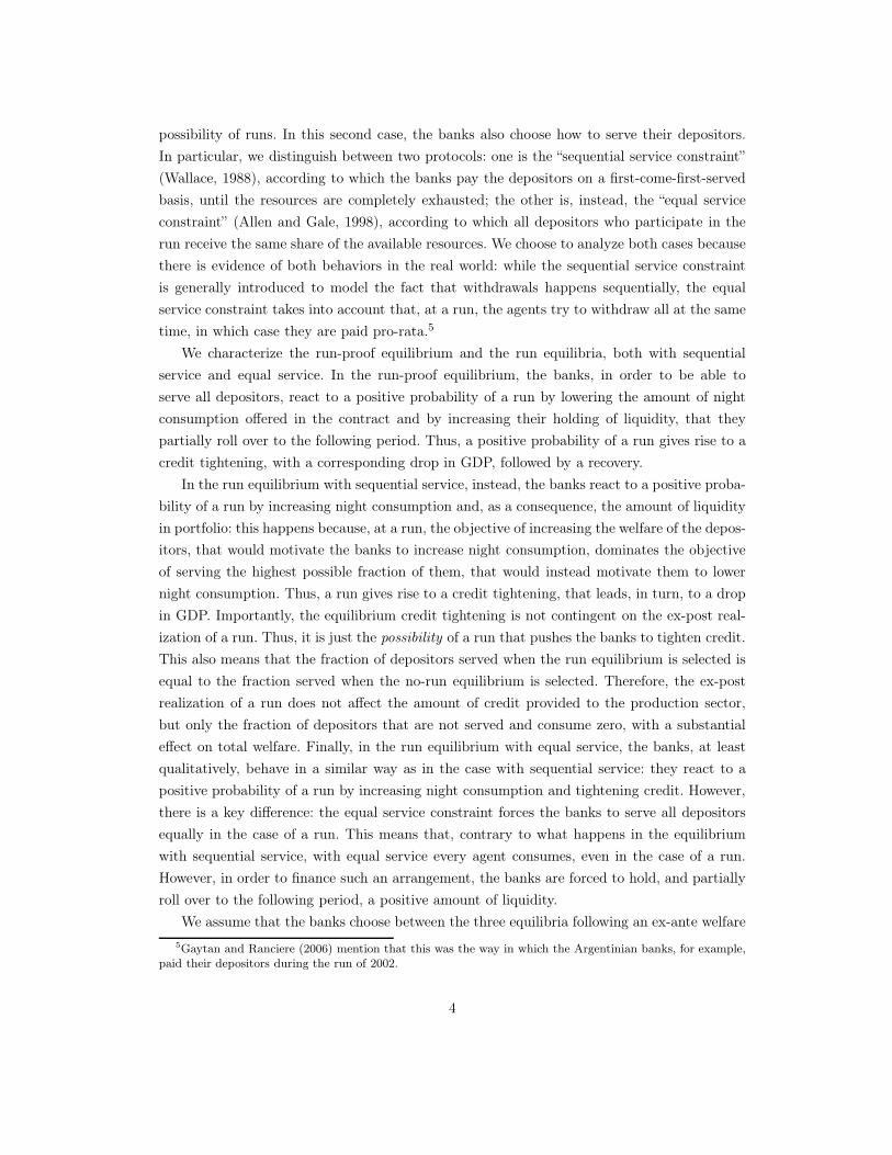
Figure 1: The impulse-response functions of run-proof equilibrium.

financial accounts.13 From here, we find that π is approximately equal to .28.14

Finally, we need to provide some reference numbers for the probability of the realization of

the sunspot q. In this respect, we take a conservative approach, and compare different values,

without any prior about what the true one is. Specifically, we show the numerical results for

a set of probabilities in the interval [0, .05], because that is the upper bound beyond which

the bank, in our simulations, chooses the run-proof contract. Hence, only for values of q lower

than that, the economy exhibits runs in equilibrium with positive probability.15

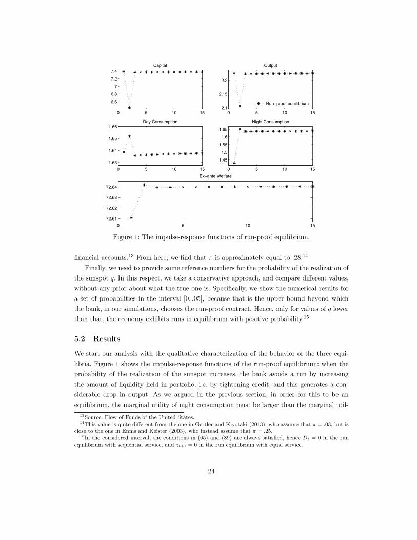
5.2 Results

We start our analysis with the qualitative characterization of the behavior of the three equi-

libria. Figure 1 shows the impulse-response functions of the run-proof equilibrium: when the

probability of the realization of the sunspot increases, the bank avoids a run by increasing

the amount of liquidity held in portfolio, i.e. by tightening credit, and this generates a con-

siderable drop in output. As we argued in the previous section, in order for this to be an

equilibrium, the marginal utility of night consumption must be larger than the marginal util-

13Source: Flow of Funds of the United States.14This value is quite different from the one in Gertler and Kiyotaki (2013), who assume that π = .03, but is

close to the one in Ennis and Keister (2003), who instead assume that π = .25.15In the considered interval, the conditions in (65) and (89) are always satisfied, hence Dt = 0 in the run

equilibrium with sequential service, and zt+1 = 0 in the run equilibrium with equal service.

24

0 5 10 156.8

77.27.4

Capital

0 5 10 152.15

2.2

Output

Sequential serviceEqual service

0 5 10 151.58

1.61.621.64

Day Consumption

0 5 10 15

1.6

1.65

1.7Night Consumption

0 5 10 15

72.63

72.64

Ex−post Welfare w/o Run

0 5 10 1520

40

60

Ex−post Welfare with Run

0 5 10 15

7171.5

7272.5

Aggregate Welfare

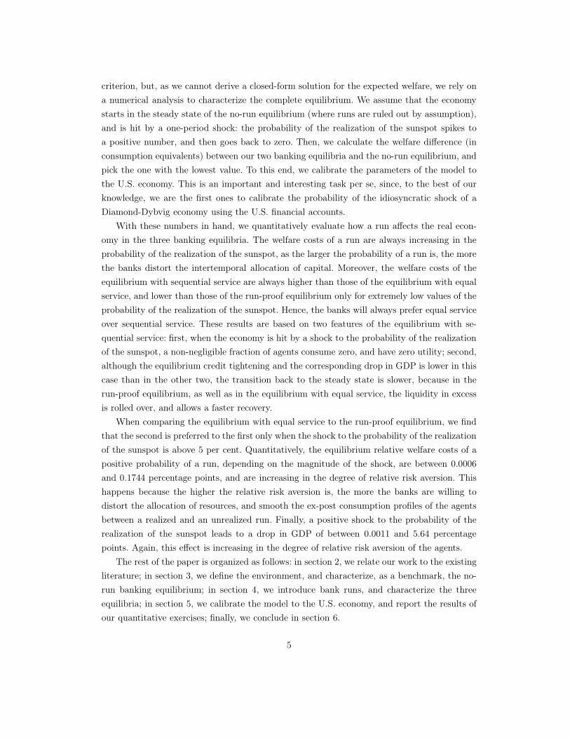
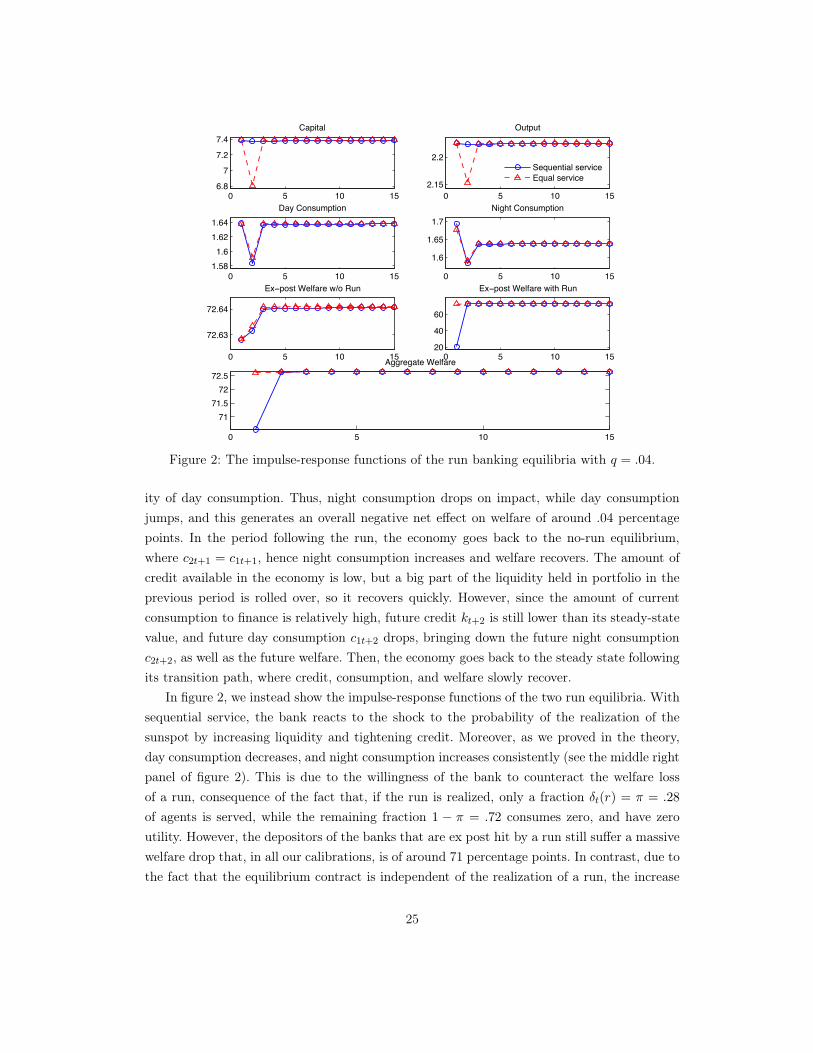
Figure 2: The impulse-response functions of the run banking equilibria with q = .04.

ity of day consumption. Thus, night consumption drops on impact, while day consumption

jumps, and this generates an overall negative net effect on welfare of around .04 percentage

points. In the period following the run, the economy goes back to the no-run equilibrium,

where c2t+1 = c1t+1, hence night consumption increases and welfare recovers. The amount of

credit available in the economy is low, but a big part of the liquidity held in portfolio in the

previous period is rolled over, so it recovers quickly. However, since the amount of current

consumption to finance is relatively high, future credit kt+2 is still lower than its steady-state

value, and future day consumption c1t+2 drops, bringing down the future night consumption

c2t+2, as well as the future welfare. Then, the economy goes back to the steady state following

its transition path, where credit, consumption, and welfare slowly recover.

In figure 2, we instead show the impulse-response functions of the two run equilibria. With

sequential service, the bank reacts to the shock to the probability of the realization of the

sunspot by increasing liquidity and tightening credit. Moreover, as we proved in the theory,

day consumption decreases, and night consumption increases consistently (see the middle right

panel of figure 2). This is due to the willingness of the bank to counteract the welfare loss

of a run, consequence of the fact that, if the run is realized, only a fraction δt(r) = π = .28

of agents is served, while the remaining fraction 1 − π = .72 consumes zero, and have zero

utility. However, the depositors of the banks that are ex post hit by a run still suffer a massive

welfare drop that, in all our calibrations, is of around 71 percentage points. In contrast, due to

the fact that the equilibrium contract is independent of the realization of a run, the increase

25

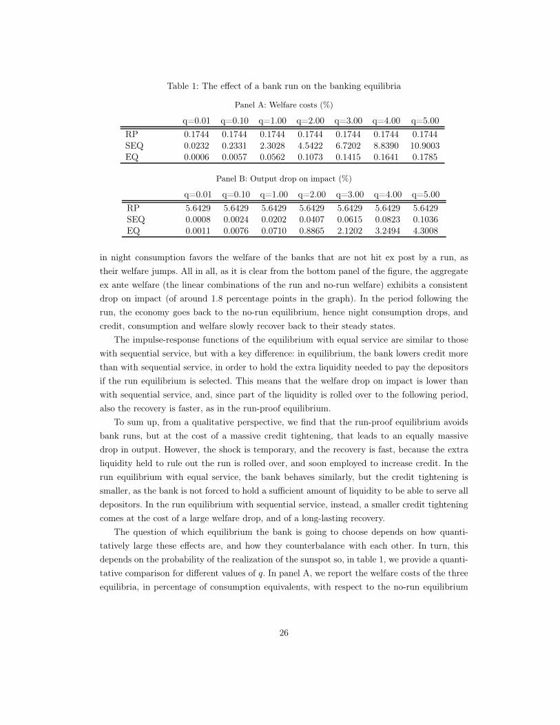
Table 1: The effect of a bank run on the banking equilibria

Panel A: Welfare costs (%)

q=0.01 q=0.10 q=1.00 q=2.00 q=3.00 q=4.00 q=5.00

RP 0.1744 0.1744 0.1744 0.1744 0.1744 0.1744 0.1744

SEQ 0.0232 0.2331 2.3028 4.5422 6.7202 8.8390 10.9003

EQ 0.0006 0.0057 0.0562 0.1073 0.1415 0.1641 0.1785

Panel B: Output drop on impact (%)

q=0.01 q=0.10 q=1.00 q=2.00 q=3.00 q=4.00 q=5.00

RP 5.6429 5.6429 5.6429 5.6429 5.6429 5.6429 5.6429

SEQ 0.0008 0.0024 0.0202 0.0407 0.0615 0.0823 0.1036

EQ 0.0011 0.0076 0.0710 0.8865 2.1202 3.2494 4.3008

in night consumption favors the welfare of the banks that are not hit ex post by a run, as

their welfare jumps. All in all, as it is clear from the bottom panel of the figure, the aggregate

ex ante welfare (the linear combinations of the run and no-run welfare) exhibits a consistent

drop on impact (of around 1.8 percentage points in the graph). In the period following the

run, the economy goes back to the no-run equilibrium, hence night consumption drops, and

credit, consumption and welfare slowly recover back to their steady states.

The impulse-response functions of the equilibrium with equal service are similar to those

with sequential service, but with a key difference: in equilibrium, the bank lowers credit more

than with sequential service, in order to hold the extra liquidity needed to pay the depositors

if the run equilibrium is selected. This means that the welfare drop on impact is lower than

with sequential service, and, since part of the liquidity is rolled over to the following period,

also the recovery is faster, as in the run-proof equilibrium.

To sum up, from a qualitative perspective, we find that the run-proof equilibrium avoids

bank runs, but at the cost of a massive credit tightening, that leads to an equally massive

drop in output. However, the shock is temporary, and the recovery is fast, because the extra

liquidity held to rule out the run is rolled over, and soon employed to increase credit. In the

run equilibrium with equal service, the bank behaves similarly, but the credit tightening is

smaller, as the bank is not forced to hold a sufficient amount of liquidity to be able to serve all

depositors. In the run equilibrium with sequential service, instead, a smaller credit tightening

comes at the cost of a large welfare drop, and of a long-lasting recovery.

The question of which equilibrium the bank is going to choose depends on how quanti-

tatively large these effects are, and how they counterbalance with each other. In turn, this

depends on the probability of the realization of the sunspot so, in table 1, we provide a quanti-

tative comparison for different values of q. In panel A, we report the welfare costs of the three

equilibria, in percentage of consumption equivalents, with respect to the no-run equilibrium

26

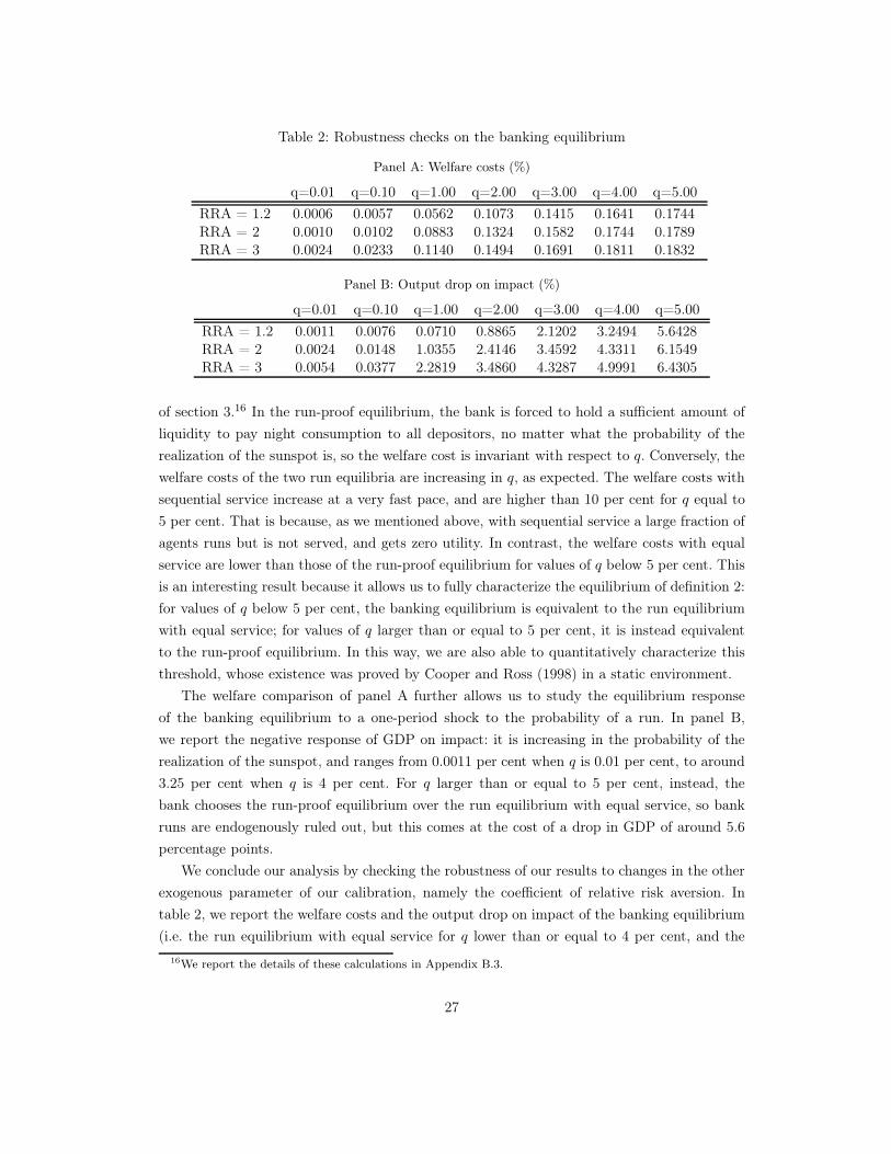
Table 2: Robustness checks on the banking equilibrium

Panel A: Welfare costs (%)

q=0.01 q=0.10 q=1.00 q=2.00 q=3.00 q=4.00 q=5.00

RRA = 1.2 0.0006 0.0057 0.0562 0.1073 0.1415 0.1641 0.1744

RRA = 2 0.0010 0.0102 0.0883 0.1324 0.1582 0.1744 0.1789

RRA = 3 0.0024 0.0233 0.1140 0.1494 0.1691 0.1811 0.1832

Panel B: Output drop on impact (%)

q=0.01 q=0.10 q=1.00 q=2.00 q=3.00 q=4.00 q=5.00

RRA = 1.2 0.0011 0.0076 0.0710 0.8865 2.1202 3.2494 5.6428

RRA = 2 0.0024 0.0148 1.0355 2.4146 3.4592 4.3311 6.1549

RRA = 3 0.0054 0.0377 2.2819 3.4860 4.3287 4.9991 6.4305

of section 3.16 In the run-proof equilibrium, the bank is forced to hold a sufficient amount of

liquidity to pay night consumption to all depositors, no matter what the probability of the

realization of the sunspot is, so the welfare cost is invariant with respect to q. Conversely, the

welfare costs of the two run equilibria are increasing in q, as expected. The welfare costs with

sequential service increase at a very fast pace, and are higher than 10 per cent for q equal to

5 per cent. That is because, as we mentioned above, with sequential service a large fraction of

agents runs but is not served, and gets zero utility. In contrast, the welfare costs with equal

service are lower than those of the run-proof equilibrium for values of q below 5 per cent. This

is an interesting result because it allows us to fully characterize the equilibrium of definition 2:

for values of q below 5 per cent, the banking equilibrium is equivalent to the run equilibrium

with equal service; for values of q larger than or equal to 5 per cent, it is instead equivalent

to the run-proof equilibrium. In this way, we are also able to quantitatively characterize this

threshold, whose existence was proved by Cooper and Ross (1998) in a static environment.

The welfare comparison of panel A further allows us to study the equilibrium response

of the banking equilibrium to a one-period shock to the probability of a run. In panel B,

we report the negative response of GDP on impact: it is increasing in the probability of the

realization of the sunspot, and ranges from 0.0011 per cent when q is 0.01 per cent, to around

3.25 per cent when q is 4 per cent. For q larger than or equal to 5 per cent, instead, the

bank chooses the run-proof equilibrium over the run equilibrium with equal service, so bank

runs are endogenously ruled out, but this comes at the cost of a drop in GDP of around 5.6

percentage points.

We conclude our analysis by checking the robustness of our results to changes in the other

exogenous parameter of our calibration, namely the coefficient of relative risk aversion. In

table 2, we report the welfare costs and the output drop on impact of the banking equilibrium

(i.e. the run equilibrium with equal service for q lower than or equal to 4 per cent, and the

16We report the details of these calculations in Appendix B.3.

27

run-proof equilibrium with q equal to 5 per cent or above) for relative risk aversion equal to 2

and 3, together with our baseline calibration. Both panel A and B show that our conclusions

are not qualitatively altered in any way: for given relative risk aversion, both the welfare costs

and the output drop are increasing in the probability of the realization of the sunspot. Ceteris

paribus, the higher the risk aversion is, the higher is the distortion of the banking equilibrium

with respect to the no-run equilibrium. This is a consequence of the fact that the more risk

averse the agents are, the less they tolerate any difference in their ex post consumption profiles,

hence the more the bank distorts the economy when the probability of the realization of the

sunspot is positive.

6 Concluding Remarks

In the present paper, we contribute to the literature on the economics of banking and crises

by studying the macroeconomic effects of systemic bank runs, in a neoclassical growth model

with a fully-microfounded banking system. Our main contribution regards the quantitative

evaluation of these effects. In particular, we are the first ones, to the best of our knowledge,

to calibrate the probability of the idiosyncratic liquidity shock, which is a standard parameter

in many theories of banking. Our findings show that the model works remarkably well from

a qualitative perspective: it predicts that a shock to the probability of a bank run leads to

a credit tightening, followed by a drop in GDP and a recovery, replicating the behavior of

many real economies in some recent crises. From a quantitative point of view, the outcomes of

the model also show that the macroeconomic effects of bank runs can be substantial, both on

GDP and on welfare. However, our findings represent only a lower bound for the effects that

systemic bank runs have on the real economy. In that sense, we need to extend it in different

directions, particularly for it to be able to replicate the kind of long-lasting recoveries that we

observe in the data.17

On a more general point, we contribute to the literature by defining and characterizing a

general-equilibrium theory of banking, that can appeal to both microeconomists and macroe-

conomists, as it bridges the microeconomic literature on banks and bank runs to a standard

macroeconomic model. This also means that we can use this setting as a starting point for

future research in many different directions. For example, we could modify the informational

structure of the banking system, to analyze the general-equilibrium dynamic effects of moral

hazard, adverse selection and asymmetric information. In a similar way, we could also extent

the macroeconomic environment, to study how the banking system interacts with the labor

market, with business-cycle fluctuations, or with monetary policy.

Finally, our work has some interesting policy implications. From the comparison between

17Following this lead, for example, Deidda and Panetti (2013) introduce bayesian learning in a macroeconomicmodel of banking and runs, and assume that, if hit by a run, a bank loses its information capital, and has tostart the learning process from zero.

28

the two service protocols, in the case when a run is realized, it is clear that stating what

the banks can or cannot do during a systemic run is key. In particular, allowing them to

choose equal service over sequential service, while generating a larger drop in GDP on impact,

seems to have a beneficial effect on the economy, in terms of a faster recovery, and of lower

intertemporal welfare costs. Moreover, the analysis of the run-proof equilibrium highlights

the fact that any regulation that rules out the incentives to run, including a fully-funded

deposit insurance scheme, is costly, both in terms of a distorted allocation of capital and of

intertemporal welfare, and is worthwhile implementing only when the probability of a run is

sufficiently high.

29

References

Allen, F. and D. Gale (1997, June). Financial Markets, Intermediaries, and Intertemporal

Smoothing. Journal of Political Economy 105 (3), 523–546.

Allen, F. and D. Gale (1998, August). Optimal Financial Crises. Journal of Finance 53 (4),

1245–1284.

Allen, F. and D. Gale (2004, July). Financial Intermediaries and Markets. Econometrica 72 (4),

1023–1061.

Angeletos, G. M., C. Hellwig, and A. Pavan (2007, May). Dynamic Global Games of Regime

Change: Learning, Multiplicity, and Timing of Attacks. Econometrica 75 (3), 711–756.

Bencivenga, V. R. and B. D. Smith (1991, April). Financial Intermediation and Endogenous

Growth. Review of Economic Studies 58 (2), 195–209.

Carlsson, H. and E. van Damme (1993, September). Global Games and Equilibrium Selection.

Econometrica 61 (5), 989–1018.

Cooper, R. and T. W. Ross (1998, February). Bank runs: Liquidity costs and investment

distortions. Journal of Monetary Economics 41 (1), 27–38.

Deidda, L. and E. Panetti (2013, December). Learning and Banking. work in progress.

Diamond, D. W. and P. H. Dybvig (1983, June). Bank Runs, Deposit Insurance, and Liquidity.

Journal of Political Economy 91 (3), 401–419.

Diamond, D. W. and R. R. Rajan (2001, April). Liquidity Risk, Liquidity Creation and

Financial Fragility: A Theory of Banking. Journal of Political Economy 109 (2), 287–327.

Ennis, H. M. and T. Keister (2003, April). Economic Growth, Liquidity, and Bank Runs.

Journal of Economic Literature 109 (2), 220–245.

Ennis, H. M. and T. Keister (2006, March). Bank runs and investment decisions revisited.

Journal of Monetary Economics 53 (2), 217–232.

Gaytan, A. and R. Ranciere (2006, October). Banks, Liquidity Crises and Economic Growth.

mimeo.

Gertler, M. and P. Karadi (2011, January). A Model of Unconventional Monetary Policy.

Journal of Monetary Economics 58 (1), 17–34.

Gertler, M. and N. Kiyotaki (2013, June). Banking, Liquidity and Bank Runs in an Infinite

Horizon Economy. NBER Working Paper No. 19129.

30

Goldstein, I. and A. Pauzner (2005, June). Demand-Deposit Contracts and the Probability of

Bank Runs. Journal of Finance 60 (3), 1293–1327.

Gorton, G. and A. Metrick (2012, January). Getting up to Speed on the Financial Crisis: A

One-Weekend-Reader’s Guide. NBER Working Paper No. 17778.

Green, E. J. and P. Lin (2003, January). Implementing efficient allocations in a model of

financial intermediation. Journal of Economic Theory 109 (1), 1–23.

Holmstrom, B. and J. Tirole (1998, February). Private and Public Supply of Liquidity. Journal

of Political Economy 106 (1), 1–40.

Jacklin, C. J. (1987). Demand Deposits, Trading Restrictions and Risk Sharing. In E. C.

Prescott and N. Wallace (Eds.), Contractual Arrangements for Intertemporal Trade, pp.

26–47. University of Minnesota Press.

Mattana, E. and E. Panetti (2014, April). Banks Runs, Investment Decisions and Asset

Markets. mimeo.

Qi, J. (1994, Summer). Bank Liquidity and Stability in an Overlapping Generation Model.

The Review of Financial Studies 7 (2), 389–417.

Reinhart, C. M. and K. S. Rogoff (2014, May). Recovery from Financial Crises: Evidence from

100 Episodes. American Economic Review 104 (5), 50–55.

Romer, P. M. (1990, October). Endogenous Technological Change. Journal of Political Econ-

omy 98 (5), S71–S102.

Wallace, N. (1988, Fall). Another attempt to explain an illiquid banking system: The Dia-

mond and Dybvig model with sequential service taken seriously. Federal Reserve Bank of

Minneapolis Quarterly Review 12, 3–16.

31

Appendices

A Microfoundations of the Banking Equilibrium

In this section, we compare the no-run banking equilibrium of section 3 with an “autarkic”

equilibrium, where the agents do not form banking coalitions to hedge against the idiosyncratic

shocks, but independently choose their portfolios of liquidity and credit to the production

sector, and adjust them, after the realization of the idiosyncratic shocks, in a secondary asset

market. More formally, the program reads:

max{x2t,x1t+1,ℓMt ,fM

t+1,kMt+1}

∞∑

t=0

βt[

πu(x2t) + β(1 − π)u(x1t+1)]

, (100)

subject to the budget constraints:

x1t + ℓMt + fMt+1 = wt +Rtkt, (101)

ℓMt + pt(fMt+1 − kMt+1) = x2t. (102)

The agents maximize their expected intertemporal welfare, subject to their budget constraints:

they invest the total per-period resources wt +Rtkt in current day consumption x1t, which is

chosen in the previous period, and in financial investment, divided in liquidity ℓMt and financial

assets fMt+1. However, differently from what happens in the banking equilibrium, the amount

of night consumption x2t is equal to the available liquidity plus the amount of financial assets

fMt+1 − kMt+1 that are not saved for the future period, and are sold in the secondary market at

price pt.

The characterization of the equilibrium starts from the equilibrium price on the secondary

market pt. It is easy to argue, following Allen and Gale (2004), that it must be the case that

pt = 1 at every point in time. The rationale for this result is based on the fact that the agents

must be ex ante indifferent between holding liquidity or not, otherwise the secondary market

does not clear. Assume, for example, that pt > 1. Then, credit yields a higher return than

liquidity, and everyone invests in it. However, if that is the case, the night consumers would

like to sell their assets in the secondary market and consume, but there would be no buyers.

Thus, the price pt would go to zero, which is a contradiction. Similarly, if pt < 1, liquidity

dominates credit, and everybody invests in it. If that is the case, the future day consumers

would like to buy assets in the secondary market, but there would be no sellers, thus the price

would go to Rt > 1, leading again to a contradiction.

The fact that the only possible equilibrium in the secondary market is one where the

agents are ex ante indifferent between holding liquidity and credit implies that their asset

portfolios are undetermined. Nevertheless, we can still use the budget constraints to solve for

32

the equilibrium allocation. Using (102) into (101), with pt = 1, we get:

x1t + x2t + kMt+1 = wt +Rtkt. (103)

Attach to this constraint the Lagrange multiplier βtλt. The first-order conditions are:

x1t+1 : (1− π)u′(x1t+1) = λt+1, (104)

x2t : πu′(x2t) = λt, (105)

kMt+1 : λt = βRt+1λt+1, (106)

Rearranging, we get:

u′(x1t) =π

1− πu′(x2t), (107)

πu′(x2t) = (1− π)βRt+1u′(x1t+1). (108)

It is evident that the market equilibrium in (107)-(108) and the banking equilibrium in (17)-

(18) are different. In a static environment, Diamond and Dybvig (1983) formally prove that

the banking equilibrium is efficient, i.e. that there is no other feasible allocation that provides

higher welfare. We claim that this result holds in our dynamic framework, too, and we show

that in a simple two-period economy.

Assume that t = 0, 1. The initial capital K0 is given, and u(c) = log(c). The production

function takes the form Yt = ZKαt K̄

1−αt , where K̄t is the total capital in the economy and

represents an externality like in Romer (1990), Z is a scale parameter, and capital fully depre-

ciates after one period. Thus, in equilibrium we have wt = (1−α)ZKt and Rt = αZ. Assume

that Z > 1/α, so that Rt > 1.

We first solve for the no-run banking equilibrium. From the budget constraint at t = 1,

we find that c11 = c21 = ZK1. The Euler equation and the budget constraint at t = 0 give:

1

ZK0 −K1=αβZ

ZK1, (109)

hence:

K1 =αβZK0

1 + αβ, (110)

c10 = c20 =ZK0

1 + αβ, (111)

c11 = c21 =αβZ2K0

1 + αβ. (112)

We now solve for the autarkic equilibrium. From the intratemporal condition (107), we have

that x21 = π1−πx11. Plug this in the budget constraint at t = 1 to obtain x11 = (1 − π)ZK1.

Finally, from the Euler equation at t = 0 and the budget constraint, we get:

π

π(ZK0 −K1)=αβZ(1− π)

(1− π)ZK1, (113)

33

which clearly gives the same allocation of capital as in the banking problem. While this is

a consequence of the assumption of log-utility, and would disappear with a CRRA felicity

function with relative risk aversion larger than 1, it is clear that the market equilibrium

provides a worse allocation of intratemporal resources than the banking equilibrium. This

is an interesting result, because it is well known that, in a static environment, the banking

equilibrium is equivalent to the market equilibrium, if we assume log-utility.

B Numerical Analysis

In this section, we provide the details of the algorithms that we use for the numerical analysis

of section 5. We let the economy reach the steady state of the no-run equilibrium of section

3, and hit it with a one-period shock to the probability of the realization of a the sunspot q.

We evaluate the evolution of the economy on impact, as well as on its trajectory back to the

steady state. In order to solve the model, we use the fact that the no-run banking equilibrium

is efficient (Diamond and Dybvig, 1983), and focus on the stationary representation of the

social planner problem.

B.1 Stationary Planner Problem With No Runs

From the resource constraint of the economy:

(1− π)c1t + πc2t +Kt+1 = Yt + (1− d)Kt, (114)

it is easy to argue that, on a balanced-growth path, all variables must growth at the same rate

g, that we back up from the production function18. Knowing that the physical capital and the

output must grow at the same rate, we find that 1+ g = (1+ γ)1/(1−α), where γ is the growth

rate of the exogenous technological process At.

We divide all variables in the problem by their own growth rate, and use the tilde to indicate

the stationary variables. If we assume a CRRA felicity function of the form u(c) = c1−1σ −1

1− 1

σ

,

with σ < 1 (so that the coefficient of relative risk aversion 1/σ is larger than 1, as we assumed),

the objective function becomes:

∞∑

t=0

βt

⎡

⎢

⎣π

(

c2t(1+g)t

(1+g)t

)1− 1σ

− 1

1− 1σ

+ β(1− π)

(

c1t+1(1+g)t+1

(1+g)t+1

)1− 1σ

− 1

1− 1σ

⎤

⎥

⎦=

=∞∑

t=0

βt

⎡

⎣πc̃1− 1

σ

2t (1 + g)t(1−1

σ)

1− 1σ

+ β(1 − π)c̃1− 1

σ

1t+1(1 + g)(t+1)(1− 1

σ)

1− 1σ

⎤

⎦−

π + β(1 − π)

(1− β)(

1− 1σ

) =

18As it is common in the literature, here we use Kt to indicate the amount of capital in the social plannerproblem.

34

=∞∑

t=0

β̃t

⎡

⎣πc̃1− 1

σ

2t

1− 1σ

+ β̃(1− π)c̃1− 1

σ

1t+1

1− 1σ

⎤

⎦−

π + β(1− π)

(1− β)(

1− 1σ

) , (115)

where β̃ = β(1+ g)1−1σ , and c̃t =

ct(1+g)t . Notice that the second part of the objective function

is a constant, and does not affect the equilibrium conditions. In a similar way, the resource

constraint becomes:

(1− π)c̃1t + πc̃2t + (1 + g)K̃t+1 = F (K̃t) + (1− d)K̃t. (116)

The planner problem is to maximize (115) subject to (116). Attach the Lagrange multiplier

β̃tλt to the resource constraint. The first-order conditions are:

c̃2t : c̃− 1

σ

2t = λt, (117)

c̃1t+1 : c̃− 1

σ

1t+1 = λt+1, (118)

K̃t+1 : (1 + g)λt = β̃[

F ′(K̃t+1) + 1− d]

λt+1. (119)

Thus, we derive the equilibrium conditions:

c̃2t = c̃1t, (120)

(1 + g)c̃− 1

σ

2t = β̃[

F ′(K̃t+1) + 1− d]

c̃− 1

σ

1t+1, (121)

c̃1t + (1 + g)K̃t+1 = F (K̃t) + (1− d)K̃t. (122)

Notice that c̃1t and K̃t are both state variables of the problem at time t. As a consequence,

the resource constraint in (122), where we use (120) to simplify the left-hand side, characterizes

the value of future capital K̃t+1. With this in hand, we derive c̃1t+1 from the Euler equation

in (121).

B.1.1 Recursive Formulation

To solve the planner problem, we often find it useful to take its recursive representation:

V (K̃t, c̃1t) =∞∑

s=0

β̃s[

πu(c̃2t+s) + β̃(1− π)u(c̃1t+1+s)]

= (123)

= πu(c̃2t) + β̃(1− π)u(c̃1t+1) + β̃πu(c̃2t+1) + β̃2(1− π)u(c̃1t+2) + · · · = (124)

= πu(c̃2t) + β̃(1− π)u(c̃1t+1) + β̃V (K̃t+1, c̃1t+1). (125)

In this way, we can write the following recursive formulation, where we drop the time under-

scripts for simplicity, and use the apex to indicate future values:

V (K̃, c̃1) = πu(c̃2) + β̃(1− π)u(c̃′1) + β̃V (K̃ ′, c̃′1). (126)

35

Then, the Bellman equation for the social planner problem reads:

V (K̃, c̃1) = maxc̃2,c̃′1,K̃

′πu(c̃2) + β̃(1− π)u(c̃′1) + β̃V (K̃ ′, c̃′1), (127)

subject to:

(1− π)c̃1 + πc̃2 + (1 + g)K̃ ′≤ F (K̃) + (1− d)K̃. (128)

Attach the Lagrange multiplier λ to the resource constraint. The first-order conditions of the

program are:

c̃2 : u′(c̃2) = λ, (129)

c̃′1 : (1− π)u′(c̃′1) + V2(K̃′, c̃′1) = 0, (130)

K̃ ′ : β̃V1(K̃′, c̃′1) = (1 + g)λ, (131)

where Vj(K̃ ′, c̃′1) is the derivative of the value function with respect to its j-th element. The

envelope conditions read:

c̃1 : V2(K̃, c̃1) = (1− π)λ, (132)

K̃ : V1(K̃, c̃1) = λ[

F ′(K̃) + 1− d]

. (133)

Thus, we derive the equilibrium conditions:

u′(c̃2) = u′(c̃1), (134)

(1 + g)u′(c̃2) = β̃[

F ′(K̃ ′) + 1− d]

u′(c̃′1). (135)

The fact that, at every point in time, the equilibrium night consumption is equal to the day

consumption greatly simplifies the quantitative analysis, because it implies that the planner

problem with no runs is observationally equivalent to the neoclassical growth model. Accord-

ingly, we solve the model using a standard value-function-iteration procedure.

B.2 Stationary Planner Problem With Runs

Following the same steps as before, we also define the stationary objective function of the

planner problem with runs. In doing this, we assume that the planner, as the banks, take as

given the available service protocols in the case that the run equilibrium is selected. Hence,

she chooses between sequential service and equal service, too. The objective function of the

stationary planner problem with sequential service reads:

∞∑

t=0

β̃t

⎡

⎣(1− q)

⎛

⎝πc̃1− 1

σ

2t

1− 1σ

+ β̃(1− π)c̃1− 1

σ

1t+1

1− 1σ

⎞

⎠+ qδ̃t(r)[

π + β(1 − π)] c̃

1− 1σ

2t

1− 1σ

⎤

⎦

−

[π + β(1− π)](1 − q + qδ̃t(r))

(1− β)(

1− 1σ

) , (136)

36

where δ̃t(r) = (ℓt + rD̃t)/c̃2t. The budget constraints, instead, are:

(1− π)c̃1t + ℓt + (1 + g)K̃t+1 + D̃t ≤ F (K̃t) + (1− d)K̃t, (137)

ℓt ≥ πc̃2t (138)

D̃t ≥ 0, (139)

K̃t+1 ≥ 0. (140)

The first-order conditions of this problem are similar to those in the text, and, with δ̃t(r) =

π and ℓt = πc̃2t, yield the equilibrium conditions:

c̃− 1

σ

2t

(

1 +q

(1− q)

[

π + β(1 − π)]

)

= c̃− 1

σ

1t , (141)

(1 + g)c̃− 1

σ

1t = β̃[

F ′(K̃t+1) + 1− d]

c̃− 1

σ

1t+1, (142)

q[

π + β(1 − π)]

rc̃− 1

σ

2t

1− 1σ

+ ηt = (1− q)c̃− 1

σ

1t . (143)

In a similar way, the objective function of the stationary planner problem with equal service

reads:

∞∑

t=0

β̃t

⎡

⎣(1− q)

⎛

⎝πc̃1− 1

σ

2t

1− 1σ

+ β̃(1− π)c̃1− 1

σ

1t+1

1− 1σ

⎞

⎠+ q[

π + β(1− π)](ℓ̃t + rD̃t)

1− 1σ

1− 1σ

⎤

⎦ (144)

−

π + β(1− π)

(1− β)(

1− 1σ

) . (145)

The bank maximizes the objective function, subject to the budget constraints:

(1− π)c̃1t + ℓ̃t + (1 + g)f̃t+1 ≤ F (K̃t) + (1− d)K̃t + z̃t, (146)

πc2t ≤ ℓt, (147)

(1 + g)K̃t+1 ≤ (1 + g)f̃t+1 − D̃t, (148)

(1 + g)z̃t+1 ≤ ℓ̃t − πc̃2t, (149)

D̃t ≥ 0, (150)

K̃t+1 ≥ 0, (151)

z̃t+1 ≥ 0. (152)

The first-order conditions of the problem yield the equilibrium conditions:

c̃− 1

σ

1t − c̃− 1

σ

2t =q

1− q

[

π + β(1− π)]

ℓ̃− 1

σ

t , (153)

(1 + g)c̃− 1

σ

1t = β̃[

F ′(K̃t+1) + 1− d]

c̃− 1

σ

1t+1, (154)

(1 + g)c̃− 1

σ

2t = β̃c̃− 1

σ

1t+1, (155)

where we used the fact that, in equilibrium, c̃R2t = ℓ̃t.

The algorithm that we use to solve the simulation is the following:19

19We use Matlab for all numerical simulations, and a standard nonlinear solver to find the solution of the

37

1. Find c̃ss and K̃ss from the steady-state equilibrium conditions of the no-run problem;

2. Solve for the transition path to the steady state of the no-run problem, using value

function iteration;

3. Use {K̃ss, c̃ss} as state variables, and derive c̃2t, c̃1t+1, f̃t+1, K̃t+1 and D̃t for the three

banking problems with runs, from the steady-state versions of the first order conditions

reported above;

4. With {K̃t+1, c̃1t+1} from the previous step as state variables, use value function iteration

to solve for the new transition path back to the steady state of the no-run banking

problem.

B.3 Welfare Costs

As already mentioned in the text, we define the welfare costs in terms of consumption equiva-

lents, i.e. as the constant percentage drop in consumption that we have to impose in order to

make the no-run banking equilibrium equivalent, in terms of welfare, to the run equilibrium.

More formally:

W(

{(1− χ)cNR2t , (1− χ)cNR

1t+1})

= W(

{ci2t, ci1t+1}

)

, (156)

where the superscript i ∈ {RP,SEQ,EQ} refers to the three equilibria that we characterized

in section 4. To simplify the notation, we define:

WNR =∞∑

t=0

β̃t

⎡

⎣πc̃1− 1

σ

2t

1− 1σ

+ β̃(1− π)c̃1− 1

σ

1t+1

1− 1σ

⎤

⎦ . (157)

Notice that WRP is equal to WNR, except for the fact that we calculate the felicity function

using {c̃RP2t , c̃RP

1t+1}. In a similar way, we also define:

W SEQ =∞∑

t=0

β̃t

⎡

⎣(1− q)

⎛

⎝πc̃1− 1

σ

2t

1− 1σ

+ β̃(1− π)c̃1− 1

σ

1t+1

1− 1σ

⎞

⎠+ qδ̃t(r)(

π + β(1− π)) c̃

1− 1

σ

2t

1− 1σ

⎤

⎦ .

(158)

Moreover:

WEQ =∞∑

t=0

β̃t

⎡

⎣(1− q)

⎛

⎝πc̃1− 1

σ

2t

1− 1σ

+ β̃(1− π)c̃1− 1

σ

1t+1

1− 1σ

⎞

⎠+ q[

π + β(1− π)] (ℓ̃t + rD̃t)

1− 1

σ

1− 1σ

⎤

⎦ .

(159)

With these in hand, we find that, for the run equilibrium with sequential service, (156) be-

comes:

(1− χSEQ)1−1

σWNR−

π + β(1− π)

(1− β)(

1− 1σ

) = W SEQ−

[π + β(1 − π)][1− q + qδ̃t(r)]

(1− β)(

1− 1σ

) , (160)

run equilibria. All codes are available upon request.

38

which gives:

χSEQ = 1−

⎡

⎢

⎣

W SEQ + q(1−δ̃t(r)])[π+β(1−π)]

(1−β)(1− 1σ)

WNR

⎤

⎥

⎦

σ

σ−1

. (161)

For the run equilibrium with equal service and for the run-proof equilibrium, instead, we get:

χEQ = 1−

[

WEQ

WNR

]

σ

σ−1

, (162)

χRP = 1−

[

WRP

WNR

]

σ

σ−1

. (163)

39

I

1|12 Public-private wage gaps in the period prior to the adoption of the euro: An ap-plication based on longitudinal data

Maria Manuel Campos | Mário Centeno

2|12 Asset pricing with a bank risk factor

João Pedro Pereira | António Rua

3|12 A wavelet-based assessment of market risk: The emerging markets case

António Rua | Luis C. Nunes

4|12 Cohesion within the euro area and the U. S.: A wavelet-based view

António Rua | Artur Silva Lopes

5|12 Excess worker turnover and fixed-term contracts: Causal evidence in a two-tier system

Mário Centeno | Álvaro A. Novo

6|12 The dynamics of capital structure decisions

Paula Antão | Diana Bonfi m

7|12 Quantile regression for long memory test-ing: A case of realized volatility

Uwe Hassler | Paulo M. M. Rodrigues | Antonio Rubia

8|12 Competition in the Portuguese Economy: An overview of classical indicators

João Amador | Ana Cristina Soares

9|12 Market perception of fiscal sustainability: An application to the largest euro area economies

Maximiano Pinheiro

10|12 The effects of public spending externalities

Valerio Ercolani | João Valle e Azevedo

11|12 Collateral requirements: Macroeconomic fluctuations and macro-prudential policy

Caterina Mendicino

12|12 Wage rigidity and employment adjust-ment at the firm level: Evidence from sur-vey data

Daniel A. Dias | Carlos Robalo Marques | Fernando Martins

13|12 How to create indices for bank branch fi-nancial performance measurement using MCDA techniques: An illustrative example

Fernando A. F. Ferreira | Paulo M. M. Rodrigues | Sérgio P. Santos | Ronald W. Spahr

14|12 On International policy coordination and the correction of global imbalances

Bruno Albuquerque | Cristina Manteu

15|12 Identifying the determinants of downward wage rigidity: some methodological con-siderations and new empirical evidence

Daniel A. Dias | Carlos Robalo Marques | Fernando Martins

16|12 Systemic risk analysis using forward-look-ing distance-to-default series

Martín Saldías

17|12 Competition in the Portuguese Economy: Insights from a profit elasticity approach

João Amador | Ana Cristina Soares

18|12 Liquidity risk in banking: Is there herding?

Diana Bonfi m | Moshe Kim

WORKING PAPERS

2012

Working Papers | 2014

II BANCO DE PORTUGAL • Working Papers

19|12 Bank size and lending specialization

Diana Bonfi m | Qinglei Dai

2013

01|13 Macroeconomic forecasting using low-frequency filters

João Valle | Azevedo, Ana Pereira

02|13 Everything you always wanted to know about sex discrimination

Ana Rute Cardoso | Paulo Guimarães | Pedro Portugal

03|13 Is there a role for domestic demand pres-sure on export performance?

Paulo Soares Esteves | António Rua

04|13 Ageing and fiscal sustainability in a small euro area economy

Gabriela Castro | José R. Maria | Ricardo Mourinho Félix | Cláudia Rodrigues Braz

05|13 Mind the gap! The relative wages of immi-grants in the Portuguese labour market

Sónia Cabral | Cláudia Duarte

06|13 Foreign direct investment and institution-al reform: Evidence and an application to Portugal

Paulo Júlio | Ricardo Pinheiro-Alves | José Tavares

07|13 Monetary policy shocks: We got news!

Sandra Gomes | Nikolay Iskrev | Caterina Mendicino

08|13 Competition in the Portuguese Economy: Estimated price-cost margins under im-perfect labour markets

João Amador | Ana Cristina Soares

09|13 The sources of wage variation: a three-way high-dimensional fixed effects regres-sion model

Sonia Torres | Pedro Portugal | John T. Addison | Paulo Guimarães

10|13 The output effects of (non-separable) gov-ernment consumption at the zero lower bound

Valerio Ercolani | João Valle e Azevedo

11|13 Fiscal multipliers in a small euro area economy: How big can they get in crisis times?

Gabriela Castro | Ricardo M. Felix | Paulo Julio | Jose R. Maria

12|13 Survey evidence on price and wage rigidi-ties in Portugal

Fernando Martins

13|13 Characterizing economic growth paths based on new structural change tests

Nuno Sobreira | Luis C. Nunes | Paulo M. M. Rodrigues

14|13 Catastrophic job destruction

Anabela Carneiro | Pedro Portugal | José Varejão

15|13 Output effects of a measure of tax shocks based on changes in legislation for Portugal

Manuel Coutinho Pereira | Lara Wemans

16|13 Inside PESSOA - A detailed description of the model

Vanda Almeida | Gabriela Castro | Ricardo M. Félix | Paulo Júlio | José R. Maria

17|13 Macroprudential regulation and macro-economic activity

Sudipto Karmakar

18|13 Bank capital and lending: An analysis of commercial banks in the United States

Sudipto Karmakar | Junghwan Mok

III

2014

1|14 Autoregressive augmentation of MIDAS regressions

Cláudia Duarte

2|14 The risk-taking channel of monetary policy – exploring all avenues

Diana Bonfi m | Carla Soares

3|14 Global value chains: Surveying drivers, measures and impacts

João Amador | Sónia Cabral

4|14 Has US household deleveraging ended? a model-based estimate of equilibrium debt

Bruno Albuquerque | Ursel Baumann | Georgi Krustev

5|14 The weather effect: Estimating the effect of voter turnout on electoral outcomes in Italy

Alessandro Sforza

6|14 Persistence in the Banking Industry: Fractional integration and breaks in memory

Uwe Hassler, Paulo M.M. Rodrigues, Antonio Rubia

7|14 Financial integration and the Great Leveraging

Daniel Carvalho

8|14 Euro Area Structural Reforms in Times of a Global Crisis

Sandra Gomes

9|14 Labour Demand Research: Towards a Better Match Between Better Theory and Better Data

John T. Addison, Pedro Portugal, José Varejão

10|14 Capital inflows and euro area long-term interest rates

Daniel Carvalho | Michael Fidora

11|14 Misallocation and productivity in the lead up to the Eurozone crisis

Daniel A. Dias | Carlos Robalo Marquesz | Christine Richmond

12|14 Global value chains: a view from the euro area

João Amador | Rita Cappariello | Robert Stehrer

13|14 A dynamic quantitative macroeconomic model of bank runs

Elena Mattana | Ettore Panetti

Working Papers | 2014