Embed Size (px)
Citation preview

Bank of Canada staff working papers provide a forum for staff to publish work-in-progress research independently from the Bank’s Governing Council. This research may support or challenge prevailing policy orthodoxy. Therefore, the views expressed in this paper are solely those of the authors and may differ from official Bank of Canada views. No responsibility for them should be attributed to the Bank.
www.bank-banque-canada.ca
Staff Working Paper/Document de travail du personnel 2017-2
A Dynamic Factor Model for Nowcasting Canadian GDP Growth
by Tony Chernis and Rodrigo Sekkel

2
Bank of Canada Staff Working Paper 2017-2
February 2017
A Dynamic Factor Model for Nowcasting Canadian GDP Growth
by
Tony Chernis1 and Rodrigo Sekkel2
1Canadian Economic Analysis Department Bank of Canada
Ottawa, Ontario, Canada K1A 0G9 [email protected]
2Financial Markets Department
Bank of Canada Ottawa, Ontario, Canada K1A 0G9
ISSN 1701-9397 © 2017 Bank of Canada
i
Acknowledgements
We are extremely thankful to Haeyeon Lee for excellent research assistance. We would also like to thank seminar participants at the Bank of Canada, the 2016 Canadian Economic Association meeting, as well as comments from André Binette, Tatjana Dahlhaus, Daniel de Munnik, Domenico Giannone, and two anonymous referees. The views expressed in this paper are solely those of the authors.

ii
Abstract
This paper estimates a dynamic factor model (DFM) for nowcasting Canadian gross domestic product. The model is estimated with a mix of soft and hard indicators, and it features a high share of international data. The model is then used to generate nowcasts, predictions of the recent past and current state of the economy. In a pseudo real-time setting, we show that the DFM outperforms univariate benchmarks as well as other commonly used nowcasting models, such as mixed-data sampling (MIDAS) and bridge regressions.
Bank topics: Econometric and statistical methods; Business fluctuations and cycles JEL codes: C38, C32, C53, E37
Résumé
Nous estimons un modèle à facteurs dynamiques (MFD) applicable à la prévision du produit intérieur brut du Canada pour la période en cours. L’estimation du modèle combine des indicateurs qualitatifs et quantitatifs et s’appuie également sur un ensemble de statistiques contenant un grand nombre de données internationales. Le modèle sert ensuite à produire des prévisions pour la période en cours, à savoir pour une période qui englobe le passé récent et la conjoncture immédiate. Dans un environnement où les données sont disponibles en temps quasi réel, nous montrons que le MFD surclasse les modèles univariés de référence ainsi que d’autres modèles fréquemment utilisés pour les prévisions de la période en cours : par exemple, les régressions fondées sur un modèle d’échantillonnage de données de fréquence mixte (MIDAS) et les modèles d’étalonnage.
Sujets : Méthodes économétriques et statistiques; Cycles et fluctuations économiques Codes JEL : C38, C32, C53, E37

Non-Technical Summary
The conduct of monetary policy, and economic policy in general, requires an assessment of the
state of the economy in real time. Macroeconomic indicators tend to be released with substantial
delays, and this is especially true for gross domestic product (GDP). To deal with this issue, policy
institutions have traditionally used simple forecasting models and judgement to predict the current
state of the economy, as well as that of the recent past. This process is now commonly referred to
as nowcasting.
In this paper, we estimate an approximate dynamic factor model (DFM) for Canada and
evaluate its nowcasting performance for Canadian GDP. DFMs are particularly appealing for
addressing the characteristic problems of nowcasting. First, there is typically a large number of
relevant variables available. Second, the release schedule can be different for each variable, which
results in unbalanced data sets. Finally, most leading indicators are monthly, while most often
the variable of interest is quarterly. Traditional models can struggle with these challenges, while a
DFM handles them elegantly.
The model developed in this paper reflects many of the distinctive characteristics of the Cana-
dian economy, and its data availability. For example, Canada releases a monthly GDP figure, and
Canadian data are released with a slightly longer lag than US data. In a pseudo real-time exercise
we show that the performance, measured by root-mean-squared forecast error, of the DFM im-
proves steadily as more information is released. We also find that US variables, such as employment
and Institute for Supply Management business surveys, are important predictors for nowcasting
Canadian GDP growth. This is because of the timely release of US variables and the importance of
the US economy for Canadian GDP growth. The model also outperforms simple benchmarks like
autoregressive models, and is competitive with other nowcasting models, such as bridge equations
and mixed-data sampling (MIDAS) regressions, especially at the nowcasting horizon.
2
1 Introduction
The conduct of monetary policy, and economic policy in general, requires an assessment of the
state of the economy in real time. Macroeconomic indicators tend to be released with substantial
delays, and this is especially true for gross domestic product (GDP). To deal with this issue, policy
institutions have traditionally used simple forecasting models and judgement to predict the current
state of the economy, as well as that of the recent past. This process is now commonly referred to
as nowcasting.
In this paper, we estimate an approximate dynamic factor model (DFM) for Canada and eval-
uate its nowcasting performance for Canadian GDP. The model developed in this paper reflects
many of the distinctive characteristics of the Canadian economy, and its data availability. Fol-
lowing Giannone et al. (2008), there is now a large literature on nowcasting with DFM. Recent
contributions include: Brazil (Bragoli et al. 2015), BRIC countries and Mexico (Dahlhaus et al.
2015), China (Giannone et al. 2013), France (Barhoumi et al. 2010), Indonesia (Luciani et al.
2015), Ireland (D’Agostino et al. 2013), New Zealand (Matheson 2010), Norway (Aastveit et al.
2011 and Luciani and Ricci 2014), and the United States (Giannone et al. 2008). A recent paper
by Bragoli and Modugno (2016) constructs a DFM for Canada that bears many similarities with
the model developed in this paper.1 These papers have shown that DFM nowcasts not only out-
perform simple benchmarks and other competing nowcasting approaches, such as bridge models
and mixed-data sampling (MIDAS) regressions, but also often produce nowcasts that are on par
with those of professional forecasters.
Dynamic factor models have also been used to study the role of specific variables for nowcasting
economic activity in a data-rich and real-time environment. Lahiri et al. (2015) study the role of
ISM business surveys in nowcasting current quarter US GDP growth, and find evidence that
these indices improve the nowcasts. Similarly, Lahiri and Monokroussos (2013) study the role
of consumer confidence in nowcasting real personal consumption expenditure in a real-time and
data-rich environment. They establish a robust link between consumer confidence and nowcast
performance for consumption in real time that is especially strong for service consumption. We
also find that the Institute for Supply Management (ISM) business survey for the United States
1We discuss in more detail the differences and similarities between the present paper and Bragoli and Modugno(2016) when we detail the model in Section 3.
3

is an important predictor for nowcasting Canadian GDP growth, given its timely release and the
importance of the US economy for Canadian GDP growth.
Through a pseudo real-time exercise using data from the first quarter of 1980 to the second
quarter of 2016, we show that the root-mean-squared forecast error (RMSFE) of the DFM improves
steadily as more information is released. The model also outperforms simple benchmarks like
autoregressive (AR) models, and is competitive with other nowcasting models, such as bridge
equations and MIDAS regressions, especially at the nowcasting horizon.
Apart from the aforementioned paper by Bragoli and Modugno (2016), there are very few
papers on nowcasting Canadian macroeconomic variables. Binette and Chang (2013) propose a
nowcasting model for Canadian GDP growth based on the Euro-STING of Camacho and Perez-
Quiros (2010). Galbraith and Tkacz (2013) examine the usefulness of payments data to nowcast
GDP growth. Relative to these papers, we contribute by proposing a different DFM, examining
a larger set of monthly and quarterly predictors, and benchmarking the results against other
nowcasting models commonly used in the literature.
The paper proceeds as follows: the next section describes our data set, followed by Section 3
that presents our dynamic factor model. Section 4 shows the performance of the DFM against
various benchmarks and the contributions of each indicator. Finally, Section 5 concludes.
2 Data
When building a nowcasting model, it is important to find variables that are: i) helpful to predict
GDP growth; ii) timely; and iii) updated frequently (e.g., monthly). To help us meet these
criteria, we choose variables that are followed by the market and reported on Statistics Canada’s
official release bulletin “The Daily.” This results in a mix of hard and soft indicators. We also
include commodity prices and a set of US economic indicators because of the Canada’s close
economic ties with the United States. Recent papers (e.g., Alvarez and Perez-Quiros 2016) that
use a similar DFM show that medium-sized data sets (i.e., with 10-30 variables) perform equally
as well as models with larger data sets with over 100 variables. With these considerations in mind,
we select 23 predictors of the Canadian economy. There are two notable peculiarities in Canadian
macroeconomic data: first, the data are released with a larger delay relative to other developed
4

economies, and second, Canada has a monthly GDP indicator. Below, we provide a more thorough
description of the variables used in the model.
The Canadian National Accounts data are released two months after the end of the reference
quarter. This means that GDP for the first quarter of the year is released at the end of May.
The monthly GDP data, denoted GDP at basic prices, have a similar lag, such that January GDP
would be released at the end of March. This is quite different from other developed countries such
as the United States and the United Kingdom, for example, who release their first estimates of
GDP four weeks after the reference period. Other European countries and Japan release their real
GDP figures with a delay of only six weeks. Furthermore, many of the most commonly used and
timely leading indicators, such as Industrial Production, are not available for Canada in a timely
manner. In the United States, Industrial Production is available within two weeks of the reference
period, while in Canada it is reported as a special aggregation of monthly real GDP data. As such,
it is released 60 days after the reference period.2
The monthly GDP at basic prices series and the quarterly GDP at market prices are distinct
measures that can have, at times, quite different growth rates. The difference lies in the treatment
of taxes and subsidies on the products.3 While production at basic prices excludes taxes and
subsidies, GDP at market prices includes them. This discrepancy can lead to significant differences
in the annualized quarterly growth between the two series, sometimes greater than 1 percentage
point in absolute value. Figure 1 illustrates that, while monthly GDP (aggregated to the quarterly
frequency) tracks quarterly GDP at market prices closely, it can deviate significantly at times.
Nonetheless, monthly GDP at basic prices is a very important predictor of quarterly GDP, and we
construct our DFM to take that into account, as detailed in the next section.
Since Canada is a small open commodity exporting economy with important trade and financial
links to the United States, our DFM includes some US indicators, as well as commodity prices and
world economic activity indicators. Of the 23 variables that we include, 14 are domestic, 6 are US
and the remaining 3 are the Bank of Canada non-energy commodity price index, WTI oil prices,
and Global Purchasing Manager’s Index (PMI).
2Canadian monthly real GDP is compiled on a by-industry basis and industrial production is an aggregation ofmining, quarrying and oil and gas extraction, utilities, manufacturing, and waste management services.
3Taxes and subsidies such as sales taxes, fuel taxes, duties and taxes on imports, excise taxes on tobacco andalcohol products and subsidies paid on agricultural commodities, transportation services and energy.
5
The domestic variables cover most of the standard nowcasting variables: car sales, PMI, mer-
chandise trade, housing variables, and various real activity measures. We also include an indicator
from the Bank of Canada’s Business Outlook Survey (BOS). The BOS is a quarterly business
survey of about 100 firms across Canada that reflects the diverse composition of the Canadian
economy in terms of region, type of business activity and firm size.4 Specifically, we use the bal-
ance of opinion on the future sales question, which has been shown to be useful in forecasting GDP
growth (Pichette and Rennison 2011).
Finally, we turn to the foreign variables. Since the United States is such an important trading
partner for Canada, we include several indicators of US economic activity in our DFM, such as
US PMI,5 and a set of standard real activity indicators, such as industrial production, retail sales
and non-farm payroll.
We transform the series to ensure stationarity. Table 1 shows all the monthly and quarterly
series, and their transformation. Furthermore, several series published by Statistics Canada have
been re-based or undergone definitional changes, which makes finding series with a sufficiently long
history difficult. To overcome this obstacle, series that suffer from this problem are simply spliced
together with the corresponding older series.
3 Econometric Framework
We follow the approach proposed by Giannone et al. (2008), with the maximum likelihood estima-
tion methodology of Banbura and Modugno (2014), which allows for arbitrary patterns of missing
data. Doz et al. (2012) study the asymptotic properties of quasi-maximum likelihood estimation
for large approximate DFMs. The authors find that the maximum likelihood estimates of the
factors are consistent, as the size of the cross-section and sample go to infinity along any path.
Furthermore, the estimator is robust to a limited degree of cross-sectional and serial correlation of
the error terms. This is particularly interesting because in large panels the assumption of no cross-
correlation could be too restrictive. We use a block factor structure similar to what is developed
in Banbura et al. (2011).
4See Martin (2004) for a detailed exposition of the Bank of Canada Business Outlook Survey.5Lahiri and Monokroussos (2013) show US PMI is a useful leading indicator for economic activity.
6

First, our model obeys the factor model representation:
yt = Λft + εt, (1)
where yt = (y1,t, y2,t, . . . , yn,t) is a set of standardized monthly stationary variables, ft denotes a
vector of r unobserved factors, and Λ is a vector of loadings.
ft = A1ft−1 + . . .+ Apft−p + ut, ut ∼ i.i.d.N(0, Q), (2)
and A1, . . . , Ap are r × r matrix of autoregressive coefficients.
Finally, we assume that the i-th idiosyncratic component of the monthly variables follows an
AR(1) process:
εi,t = αiεi,t−1 + εi,t, εi,t ∼ i.i.d.N(0, σ2i ), (3)
with E[εi,tεj,s] = 0 for i 6= j.
3.1 Quarterly Series
Quarterly series are incorporated into the model by expressing them in terms of their partially
observed monthly counterparts, as in Mariano and Murasawa (2003). Quarterly variables, like
GDP (GDPQt ), are expressed as the sum of their unobserved monthly contributions (GDPM
t ):
GDPQt = GDPM
t +GDPMt−1 +GDPM
t−2, (4)
for t = 3, 6, 9, .... define Y Qt = 100 × log(GDPQ
t ) and Y Mt = 100 × log(GDPM
t ). The unob-
served monthly rate of GDP growth, yt = ∆Y Mt , is also assumed to follow the same factor model
representation as the monthly variables:
yt = ΛQft + εQt (5)
εQt = αQεQt−1 + εQt (6)
where εQt is an i.i.d.N(0, σ2Q) process.
7
To link yt with the observed quarterly GDP series, we construct a partially observed monthly
series:
yQt =
YQt − Yt−3 , t = 3, 6, 9
unobserved , otherwise
and use the approximation of Mariano and Murasawa (2003) to obtain:
yQt = Y Qt − Y
Qt−3 ≈ (Y M
t + Y Mt−1 + Y M
t−2)− (Y Mt−3 + Y M
t−4 + Y Mt−5)
= yt + 2yt−1 + 3yt−2 + 2yt−3 + yt−4. (7)
3.2 Impact of New Data Releases
Nowcasters are frequently interested in the impact of each new data point. For example, it might
be interesting to know what the impact of the latest industrial production figure is for the GDP
forecast. Furthermore, the nowcasting environment is characterized by a large set of variables that
can arrive at a high frequency. This results in the nowcaster studying a sequence of nowcasts that
can be updated very frequently, reflecting the steady stream of new information arriving. The
DFM framework used in this paper and developed by Giannone et al. (2008) allows us to study
this so-called “news.” As discussed in Banbura et al. (2011), by analyzing the forecast revision, we
have a way of quantifying the change in information set and the average impact of each variable.
Let Ωv denote a vintage of data available at time v, where v refers to the date of a particular
data release. Since data are constantly arriving, Ωv expands throughout the nowcast period.
Furthermore, let us denote GDP growth at time t as yQt .
In this context, we can decompose a new forecast into two components.
E[yQt |Ωv+1
]︸ ︷︷ ︸
new forecast
= E[yQt |Ωv
]︸ ︷︷ ︸old forecast
+E[yQt |Iv+1
]︸ ︷︷ ︸
revision
, (8)
where Iv+1 is the subset of the set Ωv+1 that is orthogonal to all the elements of Ωv. As specified
above, the change in nowcast is due to the unexpected part of the new data release, which is called
the “news.” The news is useful because what matters in understanding the updating process of the
nowcast is not the release itself but the difference between the release and the previous forecast.
8
Hence, the effect of the news is given by
E[yQt |Ωv+1
]− E
[yQt |Ωv
]︸ ︷︷ ︸
forecast revision
=∑j∈Jv+1
bj,t,v+1
(xj,Tj,v+1
− E[xj,Tj,v+1
|Ωv
])︸ ︷︷ ︸
news
, (9)
where bj,t,v+1 are weights obtained from the model estimation and J is the set of new variables. The
nowcast revision is a combination of the news associated with the data release for each variable and
its relevancy for the target variable (quantified by its weight bj,t,v+1). This decomposition allows
the nowcaster to trace forecast revisions back to unexpected movements in individual predictors.
3.3 Estimation
We estimate the model parameters by maximum likelihood using the implementation of the Ex-
pectation Maximization (EM) algorithm proposed by Banbura and Modugno (2014). This imple-
mentation can deal with arbitrary patterns of missing observations.
An additional advantage of the maximum likelihood approach is that it easily allows us to
impose restrictions on the parameters. This feature is especially appealing in the case of Canada,
as it makes possible the addition of a factor that solely loads on the monthly and quarterly GDP
series. Bork (2009) and Bork et al. (2009) show how to impose restrictions in the model described
above. We assume that there are two factors that relate to quarterly GDP, monthly GDP and the
remaining macroeconomic and financial indicators, as follows:
1. f1,t is the factor that captures the co-movement among quarterly GDP, monthly GDP at
basic prices and all other monthly series;
2. f2,t is the factor that solely loads on quarterly and monthly GDP at basic prices.
The block factor structure implies the following properties of the transition equation (2), where
the subscript refers to the factors described above.
ft =
f1,t
f2,t
, A =
A1 0
0 A2
, Q =
Q1 0
0 Q2
(10)
The modelling choice above differs from the Bragoli and Modugno (2016) nowcasting model of
the Canadian economy. In their model, monthly GDP does not directly load on the factor; rather,
9

it follows a vector auto-regressive (VAR) process where it interacts with the factor in the state
equation. The forecast for quarterly GDP is then the monthly GDP forecast aggregated within
the model. Although the structure of their model is different, we share several key results, as the
next section shows.6 Our papers also differ in that we examine the performance of a DFM relative
to other nowcasting models and our benchmarks use final data, similar to the DFM.
4 Results
Since we do not have the real-time data vintages of every release, we perform a pseudo real-time
out-of-sample evaluation of our model in which we simulate the flow of data availability. We
replicate the data availability pattern by creating over 5,000 vintages of data, which simulates the
forecasting environment for every new release. Using these vintages, we update our predictions
with every new release of data. Table 1 shows the assumed order of data availability for our
empirical exercise. The model is estimated recursively and the first out-of-sample forecast is for
the first quarter of 2002. We start predicting quarter t GDP growth 30 days before the start of
the quarter. The model is then updated with every variable release until the publication of the
National Accounts for quarter t, about 60 days after the end of quarter t. Hence, we have 180 days
over which the predictions for quarter t GDP growth rate are generated.
As discussed in Section 3.3, we estimate the model with two block factors and one lag (p = 1)
in the VAR driving the dynamics of those factors. Finally, as specified in equation (3), we allow
the idiosyncratic components to follow an AR(1) process.
As a first pass, we benchmark the DFM forecasts with two different versions of simple AR
models. The first one, which we denote the quarterly AR, is simply an AR model with quarterly
GDP data.
yQt = α +
p∑i=1
ρiyQt−i + εt+h (11)
As discussed earlier, Canada releases data for a monthly GDP series. Thus, we also estimate
a monthly AR model, whose monthly forecasts we then aggregate into a quarterly figure.
yMt+h = α +
p∑i=1
ρiyMt−i + εt+h, (12)
6Specifically, the importance of US variables for forecasting and nowcasting.
10

where h = 1, 2, ..., 6 months, depending on which month of the quarter the forecasts are being
made.
Figure 2 shows the RMSFE of the model over the 180 days it generates predictions for quarter
t GDP. The red line shows the RMSFE of the quarterly AR model, whereas the green lines show
the RMSFE of the monthly AR model. Both models are estimated with one lag, p = 1. At the
longest forecast horizon, 30 days before the start of the quarter, the DFM performs slightly better
than the AR models, with an RMSFE about 9% lower than the monthly AR model. Nonetheless,
as new data arrive, the performance of the DFM improves substantially. Over the three months of
the nowcasting horizon, the DFM improves upon the benchmarks by a large margin. For example,
at the end of the first month of quarter t, the DFM improves upon the monthly AR model by 32%,
and at the end of the second month, by 32% as well. As we move into the backcasting horizon,
three months after the beginning of quarter t, the DFM is still more accurate than the monthly
AR model for the next 30 days. Finally, at the second month of backcasting, when two months
of monthly GDP are already known, the DFM forecasts are slightly worse than the ones from the
monthly AR.
Table 2 shows the average reduction in RMSFE due to each predictor in the model for each
period that the model generates predictions. At the longest prediction horizon, before the start of
the reference quarter t, US variables releases lead to the largest reductions in RMSFE.7 US and
Global PMIs both lead to large decreases in RMSFE at 4 and 5 basis points (bps), respectively.
Also, US Industrial Production, Retail Sales and Housing Starts make important contributions to
enhancing the accuracy of the model. On the domestic variable front, the employment rate and
the terms of trade are the two releases that reduce the RMSFE the most.
As we move into the nowcasting horizon, US variables continue to play an important role in
reducing the model’s RMSFE. US PMI is the most important release at the first nowcast horizon,
and US Industrial Production is also an important release. Imports and Exports also lead to
significant decreases in RMSFE, as do Wholesale Trade, Manufacturing Sales and the Bank of
Canada Commodity Price Index. Finally, when we reach the backcasting horizon, the predictors
other than monthly GDP have very little impact on reducing the RMSFE, especially at the second
7This result is shared with Bragoli and Modugno (2016), who also find that US variables lead to the highestimprovements in accuracy earlier in the nowcasting quarter.
11
backcast, when two months of GDP at basic prices (monthly GDP) for quarter t are already
known.
To better illustrate the importance of US variables, we estimate the DFM excluding the US
variables. Figure 3 shows the RMSFE over the prediction horizon. As the analysis of Table 2
makes clear, the largest contribution of the US variables takes place during the forecasting horizon
(T-29 to T ) and the first two months of the nowcasting horizon (T to T+60 ). During these
periods, the US variables play an important role in reducing the RMSFE of the DFM. In the third
month of the nowcast, when the monthly GDP data for the first month of the quarter are released,
the performance of the DFM with and without US data is roughly equal.
As shown in Section 3.2, the DFM model can be used to decompose the news component of every
new economic release. Looking at the news provides a better understanding of the importance of
the predictors for nowcasting Canadian GDP. Figure 5 shows the average absolute forecast revision
of the models’ forecast after the release of each predictor for each month of the prediction horizon.
As the graphs clearly show, the importance of the predictors varies widely over the prediction
horizon. At the forecasting horizon, before the start of quarter t, it is clear that US macro
variables like PMI, Industrial Production and Employment affect the predictions significantly.
To some degree, these results confirm the importance of US variables discussed in the previous
section. The US variables are important because of the close economic ties between the United
States and Canada and because of the timeliness of their release relative to Canadian data, a fact
also highlighted by Bragoli and Modugno (2016). Monthly GDP, on the other hand, has an almost
negligible impact on the prediction.
As we move into the nowcasting horizon, US variables still affect Canadian GDP predictions,
as do the Canadian employment rate, terms of trade, exports and imports. Nonetheless, as we
move further into nowcasting quarter t, the importance of monthly GDP increases, especially in
the third month of the nowcasts, when monthly GDP for the first month of quarter t is released.
Finally, as we reach the backcasting horizons, the importance of the additional predictors is much
diminished. After two months of monthly GDP is known to the model, the additional predictors
hardly move the final predictions.
Finally, to further demonstrate the fit of the DFM, Figure 4 shows the predictions for quarter-
over-quarter (QoQ) GDP growth at annual rates for our out-of-sample period (first quarter of 2002
12

to second quarter of 2016) for three different horizons: at the end of the first nowcasting month, at
the end of the last nowcasting month, and at the end of the last backcasting month, right before
the release of the National Accounts. As one can easily see, the DFM gets increasingly better as
we move along the prediction horizon. At the end of the first nowcasting month, though the model
does a good job of capturing average GDP growth, it does not show the sharp fall in the fourth
quarter of 2008 or the rebound in the second quarter of 2009. At the end of the last nowcasting
month, the model does capture the sharp fall in GDP growth during that period, and even more
so in the last backcasting period, when all model predictors are known to the model.
4.1 Comparison with Other Nowcasting Models
In this section, we compare the results of the proposed dynamic factor model with other commonly
used models for nowcasting, namely bridge equations models and MIDAS regressions.
4.1.1 Bridge models
Bridge models have a long tradition in short-term forecasting, and are often used by central banks
and policy-making institutions (see Baffigi et al. 2004 and Golinelli and Parigi 2007, among many
others). This technique involves forecasting high-frequency indicators with auxiliary models, and
using the results to forecast a low-frequency target variable. Since Canada has a monthly GDP
series, we alter this procedure slightly. Instead of aggregating the high-frequency indicator to
quarterly, we simply forecast monthly GDP using that indicator and an AR term. The nowcast is
then aggregated to a quarterly frequency.
We estimate bridge models using the following specification:
ytm+h = α +
p∑i=1
ρiytm−i + β1xi,t+hm + εtm , (13)
where xi,t+h are the remaining monthly indicators. We estimate bridge models featuring one
indicator at a time, and then average all of the nowcasts for yi,t+h for a unique combined nowcast.
We use AR models to forecast the missing observations of the monthly series. We estimate a
total of 20 bridge models, one for each of the monthly series in the data set. The models are re-
estimated over the quarter as the monthly indicators are released. The forecasts are then averaged
13

with equal weights.8
4.1.2 MIDAS regressions
A more modern benchmark model is the MIDAS regression (Ghysels et al. (2006), Ghysels et al.
(2007), and Clements and Galvao (2008)). The defining feature of MIDAS models is the way
they deal with mixed frequencies. These models use a polynomial weighting function to link
high-frequency regressors onto a low-frequency regressand. This makes the MIDAS regression a
direct forecasting tool, which does not explicitly model the dynamics of the indicator. Instead,
the MIDAS directly relates future quarterly GDP to present and lagged high-frequency indicators.
This necessitates a model for each forecast horizon.
The basic model for forecasting hq quarters ahead with hq = hm/3 is:
ytq+hq = ytm+hm = β0 + β1b(Lm, θ)x(3)tm+w
+ εtm+hm , (14)
where ytm is GDP growth and x(3)tm is the corresponding skip-sampled monthly indicator, Lm is the
monthly lag operator and w = Tx − Ty. The lag polynomial b(Lm, θ) is defined as:
b(Lm, θ) =K∑k=0
c(k; θ)Lkm. (15)
The parsimonious parametrization of the lagged coefficients c(k; θ) is one of the key features of
MIDAS models. While there are several common ways to parameterize the lagged coefficients, we
choose the so-called “Beta Lag”:
c(k, θ1, θ2) =f( k
K, θ1; θ2)∑K
k=1 f( kK, θ1; θ2)
, (16)
where f(k, θ1, θ2) = kθ1−1(1−k)θ2−1Γ(θ1+θ2)Γ(θ1),Γ(θ2)
, Γ(θ) =∫∞
0e−xxθ−1dx , and parameters θ1 and θ2 govern
the shape of the distribution. This parametrization is quite general and can take various shapes
with only a few parameters. These include increasing, decreasing or hump-shaped patterns. Fur-
thermore, we restrict the last lag to be equal to zero.
8We also combine the models with inverse MSE weights. These results are shown in an online appendix, andare very similar to the equal weights.
14

The MIDAS model is estimated using nonlinear least squares (NLS) in a regression of yt onto
x(3)t−h for each forecast horizon h = 1, . . . , H. The direct forecast is given by the conditional
expectation:
yTy+h|Tx = ytm+hm = β0 + β1b(Lm, θ)x(3)tm+w
, (17)
where Tx = Ty + w is such that the most recent observations of the indicator are included in the
conditioning set of the projection. For example, if we were trying to forecast Q2 GDP and July
PMI was available, the regression would include a lead of our indicator.
Since Canada has a monthly GDP measure, it is necessary to extend the basic MIDAS model
to have multiple explanatory variables. Furthermore, we include a low-frequency AR term. The
forecasting model then becomes:
ytq+hq = ytm+hm = β0 + β1b(Lm, θ1)x(3)1,tm+w−hm
+ β2b(Lm, θ2)x(3)2,tm+w−hm
+ λytm + εtm+hm (18)
with x(3)1 being monthly GDP measured at basic prices, and x
(3)2 an additional leading indicator.
As in the bridge models, we take the same set of leading indicators, create a model with each, and
average the individual forecasts with equal weights to create the MIDAS class forecast.
4.1.3 Comparison results
Table 3 compares the RMSFE of our DFM with the two alternative models described above. We
compare the models at the end of each month prior to the monthly GDP release, when all data
except monthly GDP are known. Relative to both the bridge and MIDAS models, the DFM is more
accurate before the first release of monthly GDP. The DFM improves over the MIDAS by close
to 19% and the bridge equations by close to 28%. For the second month of the quarter the same
trend emerges; the DFM outperforms the MIDAS and bridge models by approximately 13% and
14%, respectively. It is interesting to note how close the bridge and MIDAS models are in terms of
RMSFE; it seems that in our context there are not many gains from the more complicated bridging
polynomial. This is likely because we forecast monthly GDP and then aggregate to quarterly. In
this sense, we know the proper weights and thus do not have to estimate them as in the MIDAS
regressions. At the shortest horizon, the DFM accuracy is slightly worse than that of the bridge
and MIDAS models.
15

To test for the statistical differences in the forecast performance, we apply Diebold and Mar-
iano (1995) tests of forecast accuracy. We find that differences between the performance of the
nowcasting models are not statistically significant. However, the difference in accuracy between
the DFM and the quarterly AR model is significant at most forecast horizons, as shown in Table
3.
5 Conclusion
This paper proposes a medium-sized DFM to nowcast quarterly GDP in Canada. We deviate
from the traditional DFMs used in the nowcasting literature to accommodate specificities of the
Canadian macroeconomic data availability. The model is estimated using a panel of 23 variables,
and features an additional restricted factor to properly take into account the publication of a
monthly GDP series in Canada.
In a pseudo real-time exercise, we show that the model performs well. Our proposed DFM is
more accurate than traditional simple benchmarks such as univariate AR models. It also performs
well against competing MIDAS and bridge models, which explicitly consider additional predictors,
mixed frequencies, and ragged edges.
16

References
Aastveit, K. A., K. R. Gerdrup, A. S. Jore, and L. A. Thorsrud (2011): “Nowcasting
GDP in real-time: A density combination approach,” Tech. rep., Norges Bank.
Alvarez, R. M. C. and G. Perez-Quiros (2016): “Aggregate versus disaggregate information
in dynamic factor models,” International Journal of Forecasting, 32, 680 – 694.
Baffigi, A., R. Golinelli, and G. Parigi (2004): “Bridge models to forecast the euro area
GDP,” International Journal of forecasting, 20, 447–460.
Banbura, M., D. Giannone, and L. Reichlin (2011): “Nowcasting,” in The Oxford Handbook
of Economic Forecasting, ed. by M. P. Clements and D. F. Hendry, Oxford University Press,
63–90.
Banbura, M. and M. Modugno (2014): “Maximum likelihood estimation of factor models on
datasets with arbitrary pattern of missing data,” Journal of Applied Econometrics, 29, 133–160.
Barhoumi, K., O. Darne, and L. Ferrara (2010): “Are disaggregate data useful for factor
analysis in forecasting French GDP?” Journal of Forecasting, 29, 132–144.
Binette, A. and J. Chang (2013): “CSI: A Model for Tracking Short-Term Growth in Canadian
Real GDP,” Bank of Canada Review, 2013, 3–12.
Bork, L. (2009): “Estimating US monetary policy shocks using a factor-augmented vector au-
toregression: An EM algorithm approach,” CREATES Research Paper, 11.
Bork, L., H. Dewachter, and R. Houssa (2009): “Identification of Macroeconomic Factors
in Large Panels,” CREATES Research Paper, 43.
Bragoli, D., L. Metelli, and M. Modugno (2015): “The importance of updating: Evidence
from a Brazilian nowcasting model,” OECD Journal: Journal of Business Cycle Measurement
and Analysis, 2015, 5–22.
Bragoli, D. and M. Modugno (2016): “A Nowcasting Model for Canada: Do U.S. Variables
Matter?” Finance and Economics Discussion Series.
17
Camacho, M. and G. Perez-Quiros (2010): “Introducing the euro-sting: Short-term indicator
of euro area growth,” Journal of Applied Econometrics, 25, 663–694.
Clements, M. P. and A. B. Galvao (2008): “Macroeconomic forecasting with mixed-
frequency data: Forecasting output growth in the United States,” Journal of Business & Eco-
nomic Statistics, 26, 546–554.
D’Agostino, A., K. McQuinn, and D. OBrien (2013): “Nowcasting Irish GDP,” OECD
Journal: Journal of Business Cycle Measurement and Analysis, 2012, 21–31.
Dahlhaus, T., J.-D. Guenette, and G. Vasishtha (2015): “Nowcasting BRIC+ M in Real
Time,” Tech. rep., Bank of Canada Working Paper.
Diebold, F. X. and R. S. Mariano (1995): “Comparing Predictive Accuracy,” Journal of
Business & Economic Statistics, 253–263.
Doz, C., D. Giannone, and L. Reichlin (2012): “A quasi–maximum likelihood approach for
large, approximate dynamic factor models,” Review of Economics and Statistics, 94, 1014–1024.
Galbraith, J. and G. Tkacz (2013): “Nowcasting GDP: Electronic Payments, Data Vintages
and the Timing of Data Releases,” CIRANO Working Papers.
Ghysels, E., P. Santa-Clara, and R. Valkanov (2006): “Predicting volatility: getting the
most out of return data sampled at different frequencies,” Journal of Econometrics, 131, 59–95.
Ghysels, E., A. Sinko, and R. Valkanov (2007): “MIDAS regressions: Further results and
new directions,” Econometric Reviews, 26, 53–90.
Giannone, D., S. M. Agrippino, and M. Modugno (2013): “Nowcasting China Real GDP,”
Working Paper.
Giannone, D., L. Reichlin, and D. Small (2008): “Nowcasting: The real-time informational
content of macroeconomic data,” Journal of Monetary Economics, 55, 665–676.
Golinelli, R. and G. Parigi (2007): “The use of monthly indicators to forecast quarterly GDP
in the short run: an application to the G7 countries,” Journal of Forecasting, 26, 77–94.
18

Lahiri, K. and G. Monokroussos (2013): “Nowcasting US GDP: The role of ISM business
surveys,” International Journal of Forecasting, 29, 644–658.
Lahiri, K., G. Monokroussos, and Y. Zhao (2015): “Forecasting Consumption: the Role of
Consumer Confidence in Real Time with many Predictors,” Journal of Applied Econometrics.
Luciani, M., M. Pundit, A. Ramayandi, G. Veronese, et al. (2015): “Nowcasting In-
donesia,” Tech. rep., Board of Governors of the Federal Reserve System (US).
Luciani, M. and L. Ricci (2014): “Nowcasting Norway,” International Journal of Central
Banking, 215–248.
Mariano, R. S. and Y. Murasawa (2003): “A new coincident index of business cycles based
on monthly and quarterly series,” Journal of Applied Econometrics, 18, 427–443.
Martin, M. (2004): “The Bank of Canada’s Business Outlook Survey,” Bank of Canada Review,
2004, 3–18.
Matheson, T. D. (2010): “An analysis of the informational content of New Zealand data releases:
the importance of business opinion surveys,” Economic Modelling, 27, 304–314.
Pichette, L. and L. Rennison (2011): “Extracting Information from the Business Outlook
Survey: A Principal-Component Approach,” Bank of Canada Review, 2011, 21–28.
19
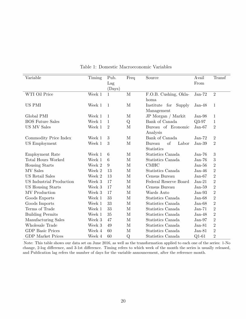
Table 1: Domestic Macroeconomic Variables
Variable Timing Pub.Lag(Days)
Freq Source AvailFrom
Transf
WTI Oil Price Week 1 1 M F.O.B. Cushing, Okla-homa
Jan-72 2
US PMI Week 1 1 M Institute for SupplyManagement
Jan-48 1
Global PMI Week 1 1 M JP Morgan / Markit Jan-98 1BOS Future Sales Week 1 1 Q Bank of Canada Q3-97 1US MV Sales Week 1 2 M Bureau of Economic
AnalysisJan-67 2
Commodity Price Index Week 1 3 M Bank of Canada Jan-72 2US Employment Week 1 3 M Bureau of Labor
StatisticsJan-39 2
Employment Rate Week 1 6 M Statistics Canada Jan-76 3Total Hours Worked Week 1 6 M Statistics Canada Jan-76 3Housing Starts Week 2 9 M CMHC Jan-56 2MV Sales Week 2 13 M Statistics Canada Jan-46 2US Retail Sales Week 2 13 M Census Bureau Jan-67 2US Industrial Production Week 3 17 M Federal Reserve Board Jan-21 2US Housing Starts Week 3 17 M Census Bureau Jan-59 2MV Production Week 3 17 M Wards Auto Jan-93 2Goods Exports Week 1 33 M Statistics Canada Jan-68 2Goods Imports Week 1 33 M Statistics Canada Jan-68 2Terms of Trade Week 1 33 M Statistics Canada Jan-71 2Building Permits Week 1 35 M Statistics Canada Jan-48 2Manufacturing Sales Week 3 47 M Statistics Canada Jan-97 2Wholesale Trade Week 3 49 M Statistics Canada Jan-81 2GDP Basic Prices Week 4 60 M Statistics Canada Jan-81 2GDP Market Prices Week 4 60 Q Statistics Canada Q1-61 2
Note: This table shows our data set on June 2016, as well as the transformation applied to each one of the series: 1-Nochange, 2-log difference, and 3-1st difference. Timing refers to which week of the month the series is usually released,and Publication lag refers the number of days for the variable announcement, after the reference month.
20

Table 2: Average Reduction in RMSFE by Variable
First First Second Third First SecondForecast Nowcast Nowcast Nowcast Backcast Backcast
WTI Oil Price 0 -2 -1 0 0 0Commodity Price Index 0 -3 0 0 0 0US PMI -4 -8 -4 0 0 0Global PMI -5 0 1 0 0 0US Employment -1 1 4 0 -1 0BOS Future Sales Growth 0 0 0 0 0 0US MV Sales 0 0 1 0 0 0Exports 2 -7 -3 -2 -2 -1Imports 0 -6 -1 1 0 0Terms of Trade -4 -1 1 -1 0 0Employment Rate -5 4 -2 -2 0 0Total Hours Worked 0 0 -3 -3 -2 -1Building Permits -1 1 0 0 0 0Housing Starts 0 -1 -1 0 0 0MV Sales -1 0 -1 0 0 0US Retail Sales -4 0 -1 0 0 1US Industrial Production -4 -3 -2 1 2 -1Manufacturing Sales 2 -1 1 1 -1 0US Housing Starts -3 0 1 -1 0 0Wholesale Trade 1 -4 -2 -1 -2 0MV Production -1 -1 3 -1 0 0GDPBP 0 -4 -4 -36 -23 -9GDP 0 0 -3 0 0 0
Note: This table shows the average reduction in RMSFE (in bps) from 2002Q1 to 2016Q2 due to eachof the variables in the DFM, and for each of the six prediction horizons.
Table 3: RMSFE of the DFM and Benchmark Models
First Fore-cast
First Now-cast
SecondNowcast
ThirdNowcast
FirstBackcast
SecondBackcast
Dynamic Factor Model 2.09 1.74 1.61 1.46* 1.05** 0.80***MIDAS 2.44 2.30 1.99 1.69* 1.19** 0.74**Bridge Equations 2.53* 2.48** 2.22* 1.67** 1.17** 0.72***Quarterly AR 2.66 2.66 2.66 2.25 2.25 2.25
Note: This table shows the RMSFE of our DFM, as well as two other commonly used nowcasting models, MIDAS andbridge models. The predictions are evaluated at the end of each month prior to the monthly GDP release, when alldata except monthly GDP are known. *, **, *** denote statistical significance at the 10, 5 and 1% level, respectively,for the Diebold-Marino test using the Quarterly AR model as the benchmark.
21
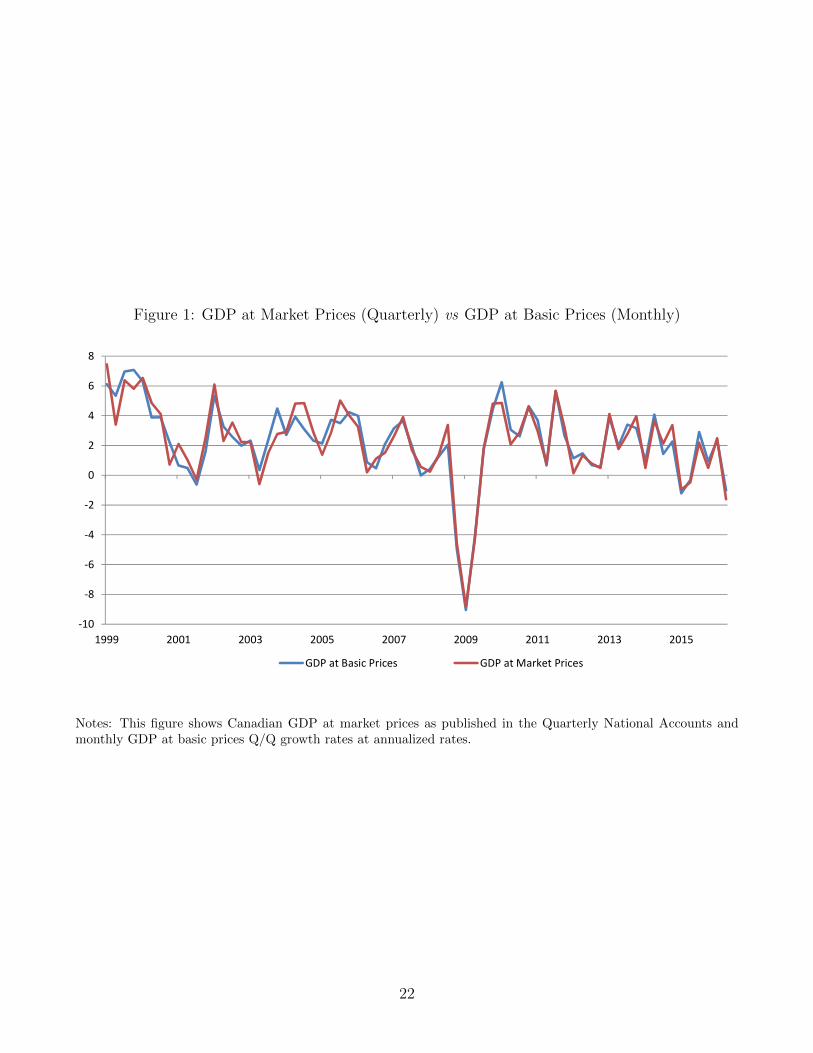
Figure 1: GDP at Market Prices (Quarterly) vs GDP at Basic Prices (Monthly)
‐10
‐8
‐6
‐4
‐2
0
2
4
6
8
1999 2001 2003 2005 2007 2009 2011 2013 2015
GDP at Basic Prices GDP at Market Prices
Notes: This figure shows Canadian GDP at market prices as published in the Quarterly National Accounts andmonthly GDP at basic prices Q/Q growth rates at annualized rates.
22

Fig
ure
2:R
MSF
Eas
New
Dat
aA
reR
elea
sed
Thro
ugh
out
the
Pre
dic
tion
Hor
izon
0
0.51
1.52
2.53
RM
SFE
Qu
arte
rly
AR
Mo
nth
ly A
R
Not
es:
Th
isfi
gure
show
sth
eR
MS
FE
ofth
eD
FM
as
new
data
are
rele
ase
dth
rou
gh
ou
tth
ep
red
icti
onh
ori
zon
.T
he
red
lin
esre
pre
sent
the
RM
SF
Eof
the
qu
arte
rly
AR
ben
chm
ark,
wh
erea
sth
egr
een
lin
esd
isp
lay
the
RM
SF
Eof
the
month
lyA
Rm
od
el.
Th
eou
t-of-
sam
ple
fore
cast
sp
erio
dru
ns
from
2002
Q1
to20
16Q
2.
23

Figure 3: RMSFE as New Data Are Released Throughout the Prediction Horizon with and withoutUS Variables
0
0.5
1
1.5
2
2.5
3
RMSFE RMSFE excluding US variables
Notes: This figure shows the RMSFE of the DFM as new data are released throughout the prediction horizon withand without the US variables.
24
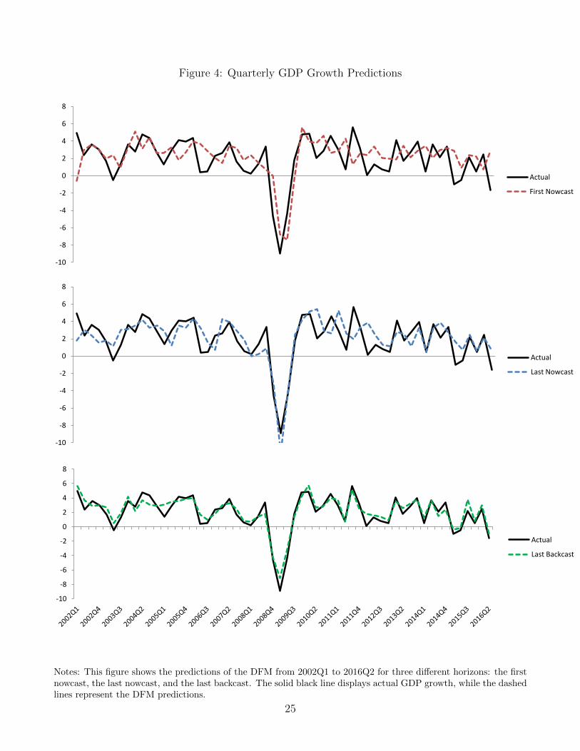
Figure 4: Quarterly GDP Growth Predictions
-10
-8
-6
-4
-2
0
2
4
6
8
Actual
Last Backcast
-10
-8
-6
-4
-2
0
2
4
6
8
Actual
Last Nowcast
-10
-8
-6
-4
-2
0
2
4
6
8
Actual
First Nowcast
Notes: This figure shows the predictions of the DFM from 2002Q1 to 2016Q2 for three different horizons: the firstnowcast, the last nowcast, and the last backcast. The solid black line displays actual GDP growth, while the dashedlines represent the DFM predictions.
25

Figure 5: Average Impact of News Releases
0
10
20
30
40
50
60
70
80
First Forecast
0
10
20
30
40
50
60
70
80
First Nowcast
0
10
20
30
40
50
60
70
80
Second Nowcast
0
10
20
30
40
50
60
70
80
Third Nowcast
0
10
20
30
40
50
60
70
80
First Backcast
0
10
20
30
40
50
60
70
80
Second Backcast
Notes: This figure shows the average absolute impact (basis points) on the forecast of every announcement in theforecast, first nowcast, second nowcast, third nowcast, as well as on the first and second backcasts.
26