Nowcasting Events from the Social Web with … · Nowcasting Events from the Social Web with Statistical Learning ... We present a general methodology for inferring the ... Nowcasting

72

Nowcasting Events from the Social Web with Statistical Learning

VASILEIOS LAMPOS and NELLO CRISTIANINI, University of Bristol, UK

We present a general methodology for inferring the occurrence and magnitude of an event or phenomenonby exploring the rich amount of unstructured textual information on the social part of the Web. Having geo-tagged user posts on the microblogging service of Twitter as our input data, we investigate two case studies.The first consists of a benchmark problem, where actual levels of rainfall in a given location and time areinferred from the content of tweets. The second one is a real-life task, where we infer regional Influenza-like Illness rates in the effort of detecting timely an emerging epidemic disease. Our analysis builds on astatistical learning framework, which performs sparse learning via the bootstrapped version of LASSO toselect a consistent subset of textual features from a large amount of candidates. In both case studies, selectedfeatures indicate close semantic correlation with the target topics and inference, conducted by regression,has a significant performance, especially given the short length –approximately one year– of Twitter’s datatime series.

Categories and Subject Descriptors: G.3 [Probability and Statistics]: Statistical computing; I.2.6 [Arti-ficial Intelligence]: Learning; I.5.4 [Pattern Recognition]: Applications—Text processing; J.3 [Life andMedical Sciences]: Medical information systems

General Terms: Algorithms, Design, Experimentation, Measurement, Performance

Additional Key Words and Phrases: Event detection, feature selection, LASSO, social network mining,sparse learning, Twitter

ACM Reference Format:Lampos, V. and Cristianini, N. 2012. Nowcasting events from the social web with statistical learning. ACMTrans. Intell. Syst. Technol. 3, 4, Article 72 (September 2012), 22 pages.DOI = 10.1145/2337542.2337557 http://doi.acm.org/10.1145/2337542.2337557

1. INTRODUCTION

It has not been a long time since snapshots of real life started to appear on the socialside of the Web. Social networks such as Facebook and Twitter have grown stronger,forming an electronic substitute for public expression and interaction. Twitter, in par-ticular, counting a total of 200 million users worldwide,1 came up with a conventionthat encouraged users to make their posts, commonly known as tweets, by default pub-licly available. Tweets being limited to a length of 140 characters (similarly to text mes-sages in mobile phones) forced their authors to produce more topic specific statements.

1Based on an email update titled as ‘Get the most out of Twitter in 2011’, sent by Twitter Inc. to its users(February 1, 2011).

V. Lampos would like to thank NOKIA Research, EPSRC (DTA/SB1826) and the Computer Science Depart-ment (University of Bristol) for all the various levels of support. N. Cristianini is supported by a RoyalSociety Wolfson Merit Award.Authors’ address: V. Lampos and N. Cristianini, Level 0, Intelligent Systems Laboratory, Merchant Ventur-ers Building, Woodland Road, BS8 1UB, Bristol, UK; email: [email protected] to make digital or hard copies of part or all of this work for personal or classroom use is grantedwithout fee provided that copies are not made or distributed for profit or commercial advantage and thatcopies show this notice on the first page or initial screen of a display along with the full citation. Copyrightsfor components of this work owned by others than ACM must be honored. Abstracting with credit is per-mitted. To copy otherwise, to republish, to post on servers, to redistribute to lists, or to use any componentof this work in other works requires prior specific permission and/or a fee. Permission may be requestedfrom Publications Dept., ACM, Inc., 2 Penn Plaza, Suite 701, New York, NY 10121-0701, USA, fax +1 (212)869-0481, or [email protected]© 2012 ACM 2157-6904/2012/09-ART72 $15.00

DOI 10.1145/2337542.2337557 http://doi.acm.org/10.1145/2337542.2337557

ACM Transactions on Intelligent Systems and Technology, Vol. 3, No. 4, Article 72, Publication date: September 2012.

72:2 V. Lampos and N. Cristianini

By adding user’s location when posting (via the mobile phone service provider or IPaddress) to this piece of public information, Twitter ushered in a new era for socialWeb media and at the same time enabled a new wave of experimentation and researchon text stream mining. Now, it has been shown that this vast amount of data encap-sulates useful signals driven by our everyday life and therefore, statistical learningmethods could be applied to extract them (several examples are provided in Section 2).

The term nowcasting, commonly used in finance, expresses the fact that we are mak-ing inferences regarding the current magnitude M(ε) of an event ε. For a time intervalu = [t − �t, t], where t denotes the current time instance, consider M

(ε(u)

)as a latent

variable. The Web content W (u) for this time interval is a partially observed variable;in particular, data from a social network, denoted as S (u) ⊆ W (u) are being observed.In this work, S (u) is used to directly infer M

(ε(u)

). For short time intervals u, we are

inferring the present value of the latent variable, that is, we are nowcasting the mag-nitude of an event. We have already presented preliminary results on a methodologyfor tracking the level of a flu epidemic from Twitter content using unigrams [Lam-pos and Cristianini 2010] and demonstrated an online tool2 for this purpose [Lamposet al. 2010]. Here we extend our previous findings and present a general frameworkfor exploiting user input published in social media.

Sparse learning enables us to select a consistent set of features (e.g., unigrams orbigrams) and then use it to perform inference via regression. The performance of theproposed methodology is evaluated by investigating two case studies. In the first, weinfer the daily amount of rainfall in five UK locations by using tweets; this forms abenchmark problem testing the limits of our approach given that rainfall has a veryinconsistent behavior in the UK [Jenkins et al. 2008]. Ground truth consists of rainfallobservations taken from weather stations located in the vicinity of the target locations.The second case study focuses on inferring the level of Influenza-like Illness (ILI) in thepopulation of three UK regions based again on geolocated Twitter content. Results arevalidated by being compared with actual ILI rates measured by the Health ProtectionAgency (HPA).3 In both case studies, experimental results are very positive in terms ofthe semantic correlation between selected features and target topics, and strong giventhe general inference performance.

The specific procedure that we followed, namely using Bolasso [Bach 2008] forfeature selection from a large set of candidates has proven to work best comparedto another relevant state-of-the-art approach [Ginsberg et al. 2008], but the generalclaim is that statistical learning techniques can be deployed for the selection offeatures and, at the same time, for the inference of a useful statistical estimator. Com-parisons with other variants of Machine Learning methods may be of interest, thoughthey would not change the main message: that one can learn the estimator from data,by means of supervised learning. In the case of ILI, other methods (e.g., Corley et al.[2009]; Polgreen et al. [2008]) propose to simply count the frequency of the diseasename. This can work well when people can diagnose their own disease (maybe easierin some cases than others) and no other confounding factors exist. However, from ourexperimental results (see Sections 5, 6, and 7), one can conclude that this is not anoptimal choice. Furthermore, it is not obvious that a function of Twitter content shouldcorrelate with the actual health state of a population. There are various possiblesampling biases that may prevent this signal from emerging. An important result ofthis study is that we find that it is possible to make up for any such bias by calibratingthe estimator on a large dataset of Twitter posts and actual HPA readings; similar

2Flu Detector, http://geopatterns.enm.bris.ac.uk/epidemics/.3HPA’s weekly epidemiological updates archive is available at http://goo.gl/wJex.


Nowcasting Events from the Social Web with Statistical Learning 72:3

results are derived for the rainfall case study. While it is true that Twitter users donot represent the general population and Twitter content might not represent anyparticular state of theirs, we find that actual states of the general population (healthor weather oriented) can be inferred as a linear function of the signal in Twitter.

The content of this article is laid out as follows: related work and background theo-retical foundations are provided in Section 2; the proposed methodology, the perfor-mance evaluation procedure and the baseline approach, to which we compare ourresults, are described in Section 3; Section 4 is concerned with the technical detailsof information collection and retrieval explaining how Twitter is sampled and also de-fines the classes of features used in our approach; Sections 5 and 6 include a detailedpresentation and analysis of the experimental results for the case studies of rainfalland flu nowcasting respectively; finally, Section 7 further discusses the derivations ofthis work, followed by the conclusions and future work in Section 8.

2. RELATED WORK AND THEORETICAL FOUNDATIONS

2.1. Related Work in Mining User-Generated Content

Recent work has been concentrated on exploiting user-generated Web content for con-ducting several types of inference. A significant subset of papers, examples of whichare given in this paragraph, focuses on methodologies that are based either on man-ually selected textual features related to a latent event, for instance, flu related key-words, or the application of sentiment/mood analysis, which in turn implies the use ofpredefined vocabularies, where words or phrases have been mapped to sentiment ormood scores [Pang and Lee 2008]. Corley et al. [2009] reported a 76.7% correlationbetween official ILI rates and the frequency of certain hand-picked influenza relatedwords in blog posts [Corley et al. 2009], whereas similar correlations were shown be-tween user search queries that included illness related words and CDC4 rates [Pol-green et al. 2008]. Furthermore, sentiment analysis has been applied in the effort ofextracting voting intentions [Tumasjan et al. 2010] or box-office revenues [Asur andHuberman 2010] from Twitter content. Similarly, mood analysis combined with a non-linear regression model derived an 87.6% correlation with daily changes in Dow JonesIndustrial Average closing values [Bollen et al. 2011]. Finally, Sakaki et al. [2010]presented a method that exploited the content, time stamp and location of a tweet todetect the existence of an earthquake.

However, in other approaches feature selection is performed automatically by ap-plying statistical learning methods. Apart from the obvious advantage of reducinghuman involvement to a minimum, those methods tend to have an improved inferenceperformance as they are enabled to explore the entire feature space or, in general, agreater amount of candidate features [Guyon and Elisseeff 2003]. In Ginsberg et al.[2008] Google researchers proposed a model able to automatically select flu relateduser search queries, which later on were used in the process of tracking ILI rates.Their method, a core component of Google Flu Trends, achieved an average correla-tion of 90% with CDC data, much higher than any other previously reported method.An extension of this approach has been applied on Twitter data achieving a 78% cor-relation with CDC rates [Culotta 2010]. In both those works, features were selectedbased on their individual correlation with ILI rates; the subset of candidate features(user search queries or keywords) appearing to independently have the highest lin-ear correlations with the target values formed the result of feature selection. Anothertechnique, part of our preliminary results, which applied sparse regression on Twit-ter content for automatic feature selection, resulted to a greater than 90% correlation

4Centers for Disease Control and Prevention (CDC), http://www.cdc.gov/.



with HPA’s flu rates for several UK regions [Lampos and Cristianini 2010]; an im-proved version of this methodology has been incorporated in Flu Detector [Lamposet al. 2010], an online tool for inferring flu rates based on tweets.

Besides minor differences regarding the information extraction and retrievaltechniques or the datasets considered, the fundamental distinction between Ginsberget al. [2008] and Culotta [2010] and Lampos and Cristianini [2010] lies on the featureselection principle; a sparse regressor, such as LASSO, does not handle each candidatefeature independently but searches for a subset of features that satisfies its constraints[Tibshirani 1996] (see Section 2.2). In this work, we extend and generalize the method-ology and preliminary results presented in Lampos and Cristianini [2010]. The maintheoretical concept is again feature selection by sparse learning, though we aim tomake this selection consistent considering, at the same time, more types of features.

2.2. Bootstrapped LASSO for Feature Selection

Least Absolute Shrinkage and Selection Operator (LASSO), presented in Tibshirani[1996], being a constrained version of ordinary least squares (OLS) regression, pro-vides a sparse regression estimate β∗ computed by solving the following optimizationproblem:

β∗ = arg minβ

N∑i=1

⎛⎝yi − β0 −

p∑j=1

xijβ j

⎞⎠

2

subject top∑

j=1

|β j| ≤ t, (1)

where x’s denote the input data (N observations of p variables), y’s are the N targetvalues, β ’s the N coefficients or weights, β0 is the regression bias and t ≥ 0 is referredto as the regularization or shrinkage parameter since it controls the regularization (orshrinkage) amount on the L1-norm of β ’s. Least Angle Regression (LARS) provides anefficient algorithm for computing the entire regularization path of LASSO [Efron et al.2004], that is, all LASSO solutions for different choices of the regularization parametert. However, it has been shown that LASSO selects more variables than necessary [Lvand Fan 2009] and that in many settings it performs an inconsistent model selection[Zhao and Yu 2006].

Bootstrap, presented in Efron [1979], was introduced as a method for assessing theaccuracy of a prediction but has also found applications in improving the predictionitself (see for example Bagging [Breiman 1996]). Suppose that we aim to fit a model toa training dataset T . The basic idea of bootstrapping is to draw n random datasets Bwith replacement from T , forcing each sample to have the same size as |T |; the drawndatasets are referred to as bootstraps. Then, refit the model into each element of Band examine the behavior of the fits [Efron and Tibshirani 1993]. The bootstrappedversion of LASSO, conventionally named as Bolasso, intersects the supports of LASSObootstrap estimates and addresses its model selection inconsistency problems [Bach2008]. Throughout this work we have applied Bolasso’s soft version (see Sections 3.1and 3.2) in our effort to select a consistent subset of textual features.

3. GENERAL METHODOLOGY

In this section, a general description of the proposed methodology is given, introducingthe notation that is going to be used throughout this script. An abstract summary ofthe methodology includes the following three main operations.

(1) Candidate Feature Extraction. A vocabulary of candidate features is formed by us-ing n-grams, that is, phrases with n tokens. We also refer to those n-grams as mark-ers. Markers are extracted from text, which is expected to contain topic-related



words, for instance, Web encyclopedias as well as other more informal references.By construction the set of extracted candidates contains many features relevantwith the target topic and much more with no direct semantic connection.

(2) Vector Space Representation. For a fixed time period and set of locations, the VectorSpace Representation (VSR) of the candidate features is computed from the textcorpus using a scheme based on Term Frequencies (TF). For the same time periodand locations, the VSR of the target topic is obtained from an authoritative source.

(3) Feature Selection and Inference. A subset of the candidate features is selected byapplying a sparse regression method. In our experiments, we have applied Bolassoto select a consistent set of features; the weights of the selected features are thenlearnt via OLS regression on the reduced input space. The selected features andtheir weights are used to perform inferences.

3.1. Formal Description

We denote the set of candidate n-grams as C = {ci}, i ∈ {1, ..., |C|}. The retrieved userposts (or tweets) for a time instance u are denoted as P (u) = {pj}, j ∈ {1, ..., |P (u)|}. Aboolean function g indicates whether a candidate marker ci is contained in a user postpj or not:

g(ci, pj) =

{1 if ci ∈ pj,0 otherwise.

(2)

Given the user posts P (u), we compute the score s of a candidate marker ci as follows:

s(ci,P (u)

)=

|P (u)|∑j=1

g(ci, pj)

|P (u)| . (3)

Therefore, the score of a candidate marker is the number of tweets containing thismarker divided by the total number of tweets for a predefined time interval. The scoresof all candidate markers for the same time interval u are kept in vector x given by:

x(u) =[s(c1,P (u)

)... s

(c|C|,P (u)

)]T. (4)

In our study, u takes the length of a day d; from this point onwards, consider a timeinterval equal to the duration of a day. However, u’s length is a matter of choicedepending on the inference task at hand.

For a set of days D = {dk}, k ∈ {1, ..., |D|} and given P (dk) ∀k, we compute the scoresof the candidate markers C. Those are held in a |D| × |C| array X (D):

X (D) =[x(d1) ... x(d|D|)

]T. (5)

For the same set of |D| days, we retrieve the values of the target variable y(D):

y(D) =[y1 ... y|D|

]T. (6)

X (D) and y(D) are used as an input in Bolasso. In each bootstrap, LASSO selects a sub-set of the candidates and at the end Bolasso, by intersecting the bootstrap outcomes,attempts to make this selection consistent. LASSO is formulated as follows:

minw

∥∥X (D)w − y(D)∥∥2

2

s.t. ‖w‖1 ≤ t,(7)



where t is the regularization parameter controlling the shrinkage of w’s L1-norm. Inturn, t can be expressed as

t = α · ‖wOLS‖1, α ∈ (0, 1], (8)

where wOLS is the OLS regression solution and a denotes the desired shrinkage percent-age of wOLS’s L1-norm. Bolasso’s implementation applies LARS, which is able to explorethe entire regularization path at the cost of one matrix inversion and decides the valueof the regularization parameter (t or α) using the largest consistent region, that is, thelargest continuous range on the regularization path, where the set of selected variablesremains the same [Efron et al. 2004].

After selecting a subset F = { fi}, i ∈ {1, ..., |F |} of the feature space, where F ⊆ C,the VSR of the initial vocabulary X (D) is reduced to an array Z (D) of size |D| × |F |. Welearn the weights of the selected features by performing OLS regression:

minws

∥∥(Z (D)ws + β

) − y(D)∥∥2

2 , (9)

where vector ws denotes the learned weights for the selected features and scalar β isregression’s bias term.

It is important to notice that statistical bounds exist linking LASSO’s expected per-formance to the one derived on the training set (empirical), the number of dimensions,number of training samples and 1-norm of w. For example in Bartlett et al. [2009] itis shown that LASSO’s expected loss L(w) up to polylogarithmic factors in W1, |C| and|D| is bounded by

L(w) ≤ L(w) + Q, with Q ∼ min{

W21

|D| +|C||D| ,

W21

|D| +W1√|D|

}, (10)

where L(w) denotes the empirical loss, |C| is the number of candidate features, |D| isthe number of training samples and W1 is an upper bound for the 1-norm of w, thatis, ‖w‖1 ≤ W1. Therefore, to minimize the prediction error using a fixed set of trainingsamples and given that the empirical error is relatively small, one should either reducethe dimensionality of the problem (|C|) or increase the shrinkage of w’s 1-norm (whichintuitively might result in sparser solutions).

3.2. Consensus Threshold and Performance Evaluation

A strict application of Bolasso implies that only features with a nonzero weight in allbootstraps are going to be considered. In our methodology a soft version of Bolasso isapplied (named as Bolasso-S in Bach [2008]), where features are considered if they ac-quire a nonzero weight in a fraction of the bootstraps, which is referred to as ConsensusThreshold (CT). CT ranges in (0, 1] and obviously is equal to 1 in the strict applicationof Bolasso. The value of CT, expressed by a percentage, is decided using a validationset. To constrain the computational complexity of the learning phase, we consider 21discrete CTs from 50% to 100% with a step of 2.5%.

Overall, performance evaluation includes three steps: (a) training, where for eachCT we retrieve a set of selected features from Bolasso and their weights from OLSregression, (b) validating CT, where we select the optimal CT value based on a valida-tion set, and (c) testing, where the performance of our previous choices is computed.Training, validation and testing sets are by definition disjoint from each other.



ALGORITHM 1: Baseline Method: Feature Selection via Correlation Analysis

Input: C1:n, X (train)[1:m,1:n], y(train)

1:m , X (val)[1:m′,1:n], y(val)

1:m′

Output: C1:p

ρ1:n ← correlation(X (train)

[1:m,1:n], y(train)1:m

);

ρ1:n ← descendingCorrelationIndex(ρ1:n);C1:n ← Cρ1:n;while i ≤ k do

Li ← validate(X (train)

[1:m,ρ1:i], y(train)

1:m , X (val)[1:m′,ρ1:i]

, y(val)1:m′

);

endp ← arg min

iLi;

return C1:p;

The Mean Squared Error (MSE) between inferred (Xw) and target values (y) formsthe loss (L) during all steps. For a sample of size |D| this is defined as:

L(w) =1

|D||D|∑i=1

� (〈xiw〉, yi), (11)

where the loss function �(〈xiw〉, yi) = (〈xiw〉 − yi)2. The Root Mean Squared Error(RMSE) – the square root of MSE – has been used as a more comprehensive metric(it has the same units with the target variables) for presenting results in Sections 5and 6.

To summarise CT’s validation, suppose that for all considered consensus thresholdsCTi, i ∈ {1, ..., 21}, training yields Fi sets of selected features respectively, whose losseson the validation set are denoted by L( val)

i . Then, if i(∗) denotes the index of the selectedCT and set of features, it is given by:

i(∗) = arg mini

L( val)i . (12)

Therefore, CTi(∗) is the result of the validation process and Fi(∗) is used in the testingphase.

Taking into consideration that both target values (rainfall and flu rates) can onlybe zero or positive, we threshold the negative inferred values with zero during testing,that is, xi ← max{xi, 0}. We perform this filtering only in the testing phase; duringCT’s validation, we want to keep track of deviations in the negative space as well.

As part of the evaluation process, we compare our results with a baseline approachthat encapsulates the methodologies in Ginsberg et al. [2008] and Culotta [2010].Those approaches, as explained in Section 2, mainly differ in the feature selection pro-cess that is performed via correlation analysis (Algorithm 1). Briefly, given a set C of ncandidate features, their computed VSRs for training and validation X (train) and X (val)

and the corresponding response values y(train) and y(val), this feature selection process:a) computes the Pearson correlation coefficients (ρ) between each candidate featureand the response values in the training set, b) ranks the retrieved correlation coeffi-cients in descending order, c) computes the OLS-fit loss (L) of incremental subsets ofthe top-k correlated terms on the validation set and d) selects the subset of candidatefeatures with the minimum loss. The inference performance of the selected features isevaluated on a (disjoint) test set.



4. DATA COLLECTION AND INFORMATION RETRIEVAL

For the experimental purposes of this work we use millions of tweets collected via Twit-ter’s Search API and ground truth from authoritative sources. Based on the fact thatinformation geolocation is a key concept in both case studies, we are considering onlytweets tagged with the location (longitude and latitude coordinates) of their author.We use UK’s 54 most populated urban centers and collect tweets geolocated within a10km range from each one of them. Our crawler exploits Atom feeds and periodicallyretrieves the 100 most recent tweets per urban center.5 The time interval between con-secutive queries for an urban center varied from 5 to 10 minutes but has been stableon a daily basis and always the same for all locations. Therefore, a sampling method iscarried out during collection; we try to reduce sampling biases (for the purposes of ourwork) by using the same sampling frequency per urban center. Collecting all tweets,apart from being a much more resource demanding process, would also have resultedin exceeding data collection limits set by Twitter. Nonetheless, the daily number ofcollected tweets (more than 200,000) is considered adequate for the experimental partof this work.

All collected tweets are stored and indexed in a MySQL database. Text preprocess-ing such as stemming by applying Porter’s Algorithm for English language [Porter1980], stop word and punctuation removal as well as the computation of VSRs areperformed by our software libraries. VSRs are formed using a TF binary vector spacemodel as already described in Section 3.1.

Candidate features, that is, the pool or vocabulary of n-grams on which feature se-lection is applied, are extracted from encyclopedic, scientific, or more informal Webreferences related to the inference topic.6 By performing feature extraction in thisway, we secure the existence of good candidate features, but we are also enabled totest the feature selection capability of our method, since most candidates are not di-rectly related to the target topic. A typical information retrieval approach would haveimplied the creation of a vocabulary index from the entire Twitter corpus [Manninget al. 2008]; our choice is extensively justified in the discussion section. Neverthe-less, acquired results indicate that our simplification in the feature extraction processresults in a significant inference performance.

4.1. Feature Classes

Three classes of candidate features have been investigated: unigrams or 1-grams (de-noted by U), bigrams or 2-grams (B) and a hybrid combination (H) of 1-grams and2-grams. 1-grams being single words cannot be characterized by a consistent semanticinterpretation in most of the topics. They take different meanings and express distinctoutcomes based on the surrounding textual context. 2-grams on the other hand canbe more focused semantically. However, their frequency in a corpus is expected to belower than the one of 1-grams. Particularly, in the Twitter corpus, which consists ofvery short pieces of text (tweets are at most 140 characters long), their occurrences areexpected to be sometimes close to zero.

The hybrid class of features exploits the advantages of classes U and B and reducesthe impact of their disadvantages. It is formed by combining the training results ofU and B for all CTs. Validation and testing are performed on the combined datasets.Suppose that for all considered consensus thresholds CTi, i ∈ {1, ..., |CT|}, 1-grams

5For an area formed by a center with coordinates –latitude and longitude– (X,Y) and a radius of R Km,the N most recent tweets written in English language are retrieved by performing the following query:http://search.twitter.com/search.atom?geocode=X,Y,R&lang=en&rpp=N.6Lists of Web references and extracted features for the investigated case studies in this article are availableat http://geopatterns.enm.bris.ac.uk/twitter/.



and 2-grams selected via Bolasso are denoted by F (U)i and F (B)

i respectively. Then, thepseudo-selected n-grams for all CTs for the hybrid class F (H)

i are formed by their union,F (H)

i ={F (U)

i ∪ F (B)i

}, i ∈ {1, ..., |CT|}. Likewise, Z (H)

i ={Z (U)

i ∪ Z (B)i

}, i ∈ {1, ..., |CT|},

where Z denotes the VSR of each feature class (using Section’s 3.1 notation). Valida-tion and testing are performed on Z (H)

i as it has already been described in Section 3.2.Note that compiling an optimal hybrid scheme is not the main focus here; our aim isto investigate whether a simple combination of 1-grams and 2-grams is able to deliverbetter results. The experimental results (see Sections 5 and 6) do indeed indicate thatfeature class H performs on average better than U and B.

5. NOWCASTING RAINFALL RATES FROM TWITTER

In the first case study, we exploit the content of Twitter to infer daily rainfall rates(measured in millimetres of precipitation) for five UK cities, namely Bristol, London,Middlesbrough, Reading and Stoke-on-Trent. The choice of those locations has beenbased on the availability of ground truth, that is, daily rainfall measurements fromweather stations installed in their vicinity.

We consider the inference of precipitation levels at a given time and place as agood benchmark problem, in that it has many of the properties of other more usefulscenarios, while still allowing us to verify the performance of the system, since rainfallis a measurable variable. The event of rain is a piece of information available to thesignificant majority of Twitter users and affects various activities that could form adiscussion topic in tweets. Furthermore, predictions about it are not always easy dueto its nonsmooth behavior [Jenkins et al. 2008].

The candidate markers for this case study are extracted from weather relatedWeb references, such as Wikipedia’s page on Rainfall, an English language courseon weather vocabulary, a page with formal weather terminology and several others.As already mentioned in Section 4, the majority of the extracted candidate featuresis not directly related to the target topic, but there exists a subset of markers thatcould probably offer a good semantic interpretation. Markers with a count ≤ 10 in theTwitter corpus used for this case study are removed. Hence, from the extracted 23811-grams, 2159 have been kept as candidates; likewise the 7757 extracted 2-grams havebeen reduced to 930.

5.1. Experimental Settings

A year of Twitter data and rainfall observations (from the July 1, 2009 to the June30, 2010) formed the input data for this experiment. For this time period and theconsidered locations, 8.5 million tweets have been collected. In each run of Bolasso thenumber of bootstraps is proportional to the size of the training sample (approximately13% using the same principle as in Bach [2008]), and in every bootstrap we select atmost 300 features by performing at most 900 iterations. A bootstrap is completed assoon as one of those two stopping criteria is met. This is an essential trade-off thatguarantees a quicker execution of the learning phase, especially when dealing withlarge amounts of data.

The performance of each feature class is computed by applying a 6-fold cross valida-tion. Each fold is based on 2 months of data starting from the month pair July-August(2009) and ending with May-June (2010). In every step of the cross validation, 5folds are used for training, the first half (a month-long data) of the remaining fold forvalidating CT and the second half for testing the performance of the selected markersand their weights. Training is performed by using the VSRs of all five locations in



Table I.

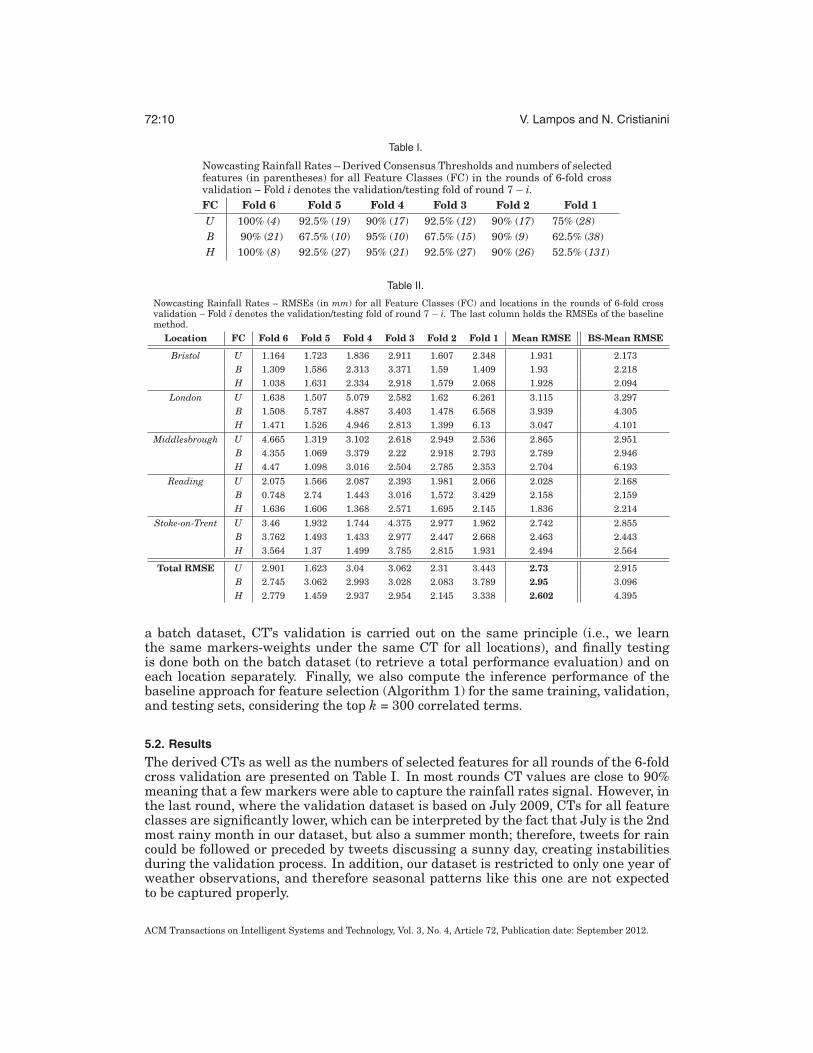
Nowcasting Rainfall Rates – Derived Consensus Thresholds and numbers of selectedfeatures (in parentheses) for all Feature Classes (FC) in the rounds of 6-fold crossvalidation – Fold i denotes the validation/testing fold of round 7 − i.FC Fold 6 Fold 5 Fold 4 Fold 3 Fold 2 Fold 1U 100% (4) 92.5% (19) 90% (17) 92.5% (12) 90% (17) 75% (28)B 90% (21) 67.5% (10) 95% (10) 67.5% (15) 90% (9) 62.5% (38)H 100% (8) 92.5% (27) 95% (21) 92.5% (27) 90% (26) 52.5% (131)

Table II.

Nowcasting Rainfall Rates – RMSEs (in mm) for all Feature Classes (FC) and locations in the rounds of 6-fold crossvalidation – Fold i denotes the validation/testing fold of round 7 − i. The last column holds the RMSEs of the baselinemethod.

Location FC Fold 6 Fold 5 Fold 4 Fold 3 Fold 2 Fold 1 Mean RMSE BS-Mean RMSE

Bristol U 1.164 1.723 1.836 2.911 1.607 2.348 1.931 2.173B 1.309 1.586 2.313 3.371 1.59 1.409 1.93 2.218H 1.038 1.631 2.334 2.918 1.579 2.068 1.928 2.094

London U 1.638 1.507 5.079 2.582 1.62 6.261 3.115 3.297B 1.508 5.787 4.887 3.403 1.478 6.568 3.939 4.305H 1.471 1.526 4.946 2.813 1.399 6.13 3.047 4.101

Middlesbrough U 4.665 1.319 3.102 2.618 2.949 2.536 2.865 2.951B 4.355 1.069 3.379 2.22 2.918 2.793 2.789 2.946H 4.47 1.098 3.016 2.504 2.785 2.353 2.704 6.193

Reading U 2.075 1.566 2.087 2.393 1.981 2.066 2.028 2.168B 0.748 2.74 1.443 3.016 1.572 3.429 2.158 2.159H 1.636 1.606 1.368 2.571 1.695 2.145 1.836 2.214

Stoke-on-Trent U 3.46 1.932 1.744 4.375 2.977 1.962 2.742 2.855B 3.762 1.493 1.433 2.977 2.447 2.668 2.463 2.443H 3.564 1.37 1.499 3.785 2.815 1.931 2.494 2.564

Total RMSE U 2.901 1.623 3.04 3.062 2.31 3.443 2.73 2.915B 2.745 3.062 2.993 3.028 2.083 3.789 2.95 3.096H 2.779 1.459 2.937 2.954 2.145 3.338 2.602 4.395

a batch dataset, CT’s validation is carried out on the same principle (i.e., we learnthe same markers-weights under the same CT for all locations), and finally testingis done both on the batch dataset (to retrieve a total performance evaluation) and oneach location separately. Finally, we also compute the inference performance of thebaseline approach for feature selection (Algorithm 1) for the same training, validation,and testing sets, considering the top k = 300 correlated terms.

5.2. Results

The derived CTs as well as the numbers of selected features for all rounds of the 6-foldcross validation are presented on Table I. In most rounds CT values are close to 90%meaning that a few markers were able to capture the rainfall rates signal. However, inthe last round, where the validation dataset is based on July 2009, CTs for all featureclasses are significantly lower, which can be interpreted by the fact that July is the 2ndmost rainy month in our dataset, but also a summer month; therefore, tweets for raincould be followed or preceded by tweets discussing a sunny day, creating instabilitiesduring the validation process. In addition, our dataset is restricted to only one year ofweather observations, and therefore seasonal patterns like this one are not expectedto be captured properly.



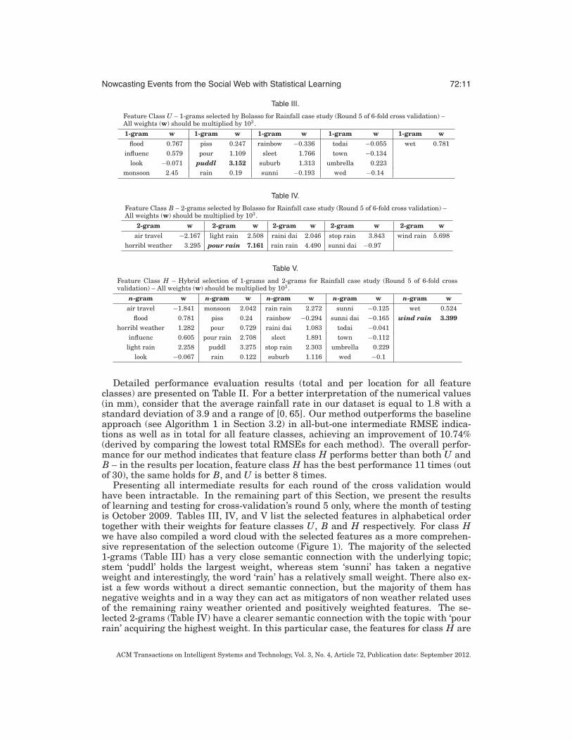
Table III.

Feature Class U – 1-grams selected by Bolasso for Rainfall case study (Round 5 of 6-fold cross validation) –All weights (w) should be multiplied by 103.

1-gram w 1-gram w 1-gram w 1-gram w 1-gram wflood 0.767 piss 0.247 rainbow −0.336 todai −0.055 wet 0.781

influenc 0.579 pour 1.109 sleet 1.766 town −0.134look −0.071 puddl 3.152 suburb 1.313 umbrella 0.223

monsoon 2.45 rain 0.19 sunni −0.193 wed −0.14

Table IV.

Feature Class B – 2-grams selected by Bolasso for Rainfall case study (Round 5 of 6-fold cross validation) –All weights (w) should be multiplied by 103.

2-gram w 2-gram w 2-gram w 2-gram w 2-gram wair travel −2.167 light rain 2.508 raini dai 2.046 stop rain 3.843 wind rain 5.698

horribl weather 3.295 pour rain 7.161 rain rain 4.490 sunni dai −0.97

Table V.

Feature Class H – Hybrid selection of 1-grams and 2-grams for Rainfall case study (Round 5 of 6-fold crossvalidation) – All weights (w) should be multiplied by 103.

n-gram w n-gram w n-gram w n-gram w n-gram wair travel −1.841 monsoon 2.042 rain rain 2.272 sunni −0.125 wet 0.524

flood 0.781 piss 0.24 rainbow −0.294 sunni dai −0.165 wind rain 3.399horribl weather 1.282 pour 0.729 raini dai 1.083 todai −0.041

influenc 0.605 pour rain 2.708 sleet 1.891 town −0.112light rain 2.258 puddl 3.275 stop rain 2.303 umbrella 0.229

look −0.067 rain 0.122 suburb 1.116 wed −0.1

Detailed performance evaluation results (total and per location for all featureclasses) are presented on Table II. For a better interpretation of the numerical values(in mm), consider that the average rainfall rate in our dataset is equal to 1.8 with astandard deviation of 3.9 and a range of [0, 65]. Our method outperforms the baselineapproach (see Algorithm 1 in Section 3.2) in all-but-one intermediate RMSE indica-tions as well as in total for all feature classes, achieving an improvement of 10.74%(derived by comparing the lowest total RMSEs for each method). The overall perfor-mance for our method indicates that feature class H performs better than both U andB – in the results per location, feature class H has the best performance 11 times (outof 30), the same holds for B, and U is better 8 times.

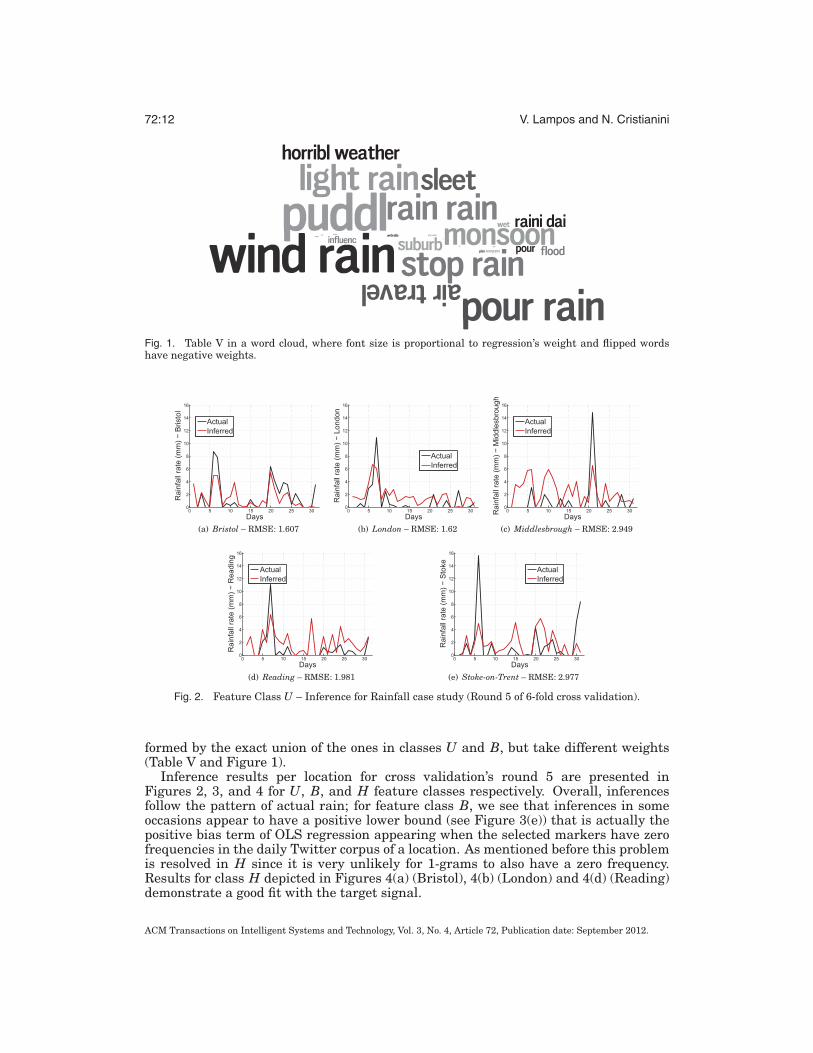
Presenting all intermediate results for each round of the cross validation wouldhave been intractable. In the remaining part of this Section, we present the resultsof learning and testing for cross-validation’s round 5 only, where the month of testingis October 2009. Tables III, IV, and V list the selected features in alphabetical ordertogether with their weights for feature classes U, B and H respectively. For class Hwe have also compiled a word cloud with the selected features as a more comprehen-sive representation of the selection outcome (Figure 1). The majority of the selected1-grams (Table III) has a very close semantic connection with the underlying topic;stem ‘puddl’ holds the largest weight, whereas stem ‘sunni’ has taken a negativeweight and interestingly, the word ‘rain’ has a relatively small weight. There also ex-ist a few words without a direct semantic connection, but the majority of them hasnegative weights and in a way they can act as mitigators of non weather related usesof the remaining rainy weather oriented and positively weighted features. The se-lected 2-grams (Table IV) have a clearer semantic connection with the topic with ‘pourrain’ acquiring the highest weight. In this particular case, the features for class H are



Fig. 1. Table V in a word cloud, where font size is proportional to regression’s weight and flipped wordshave negative weights.

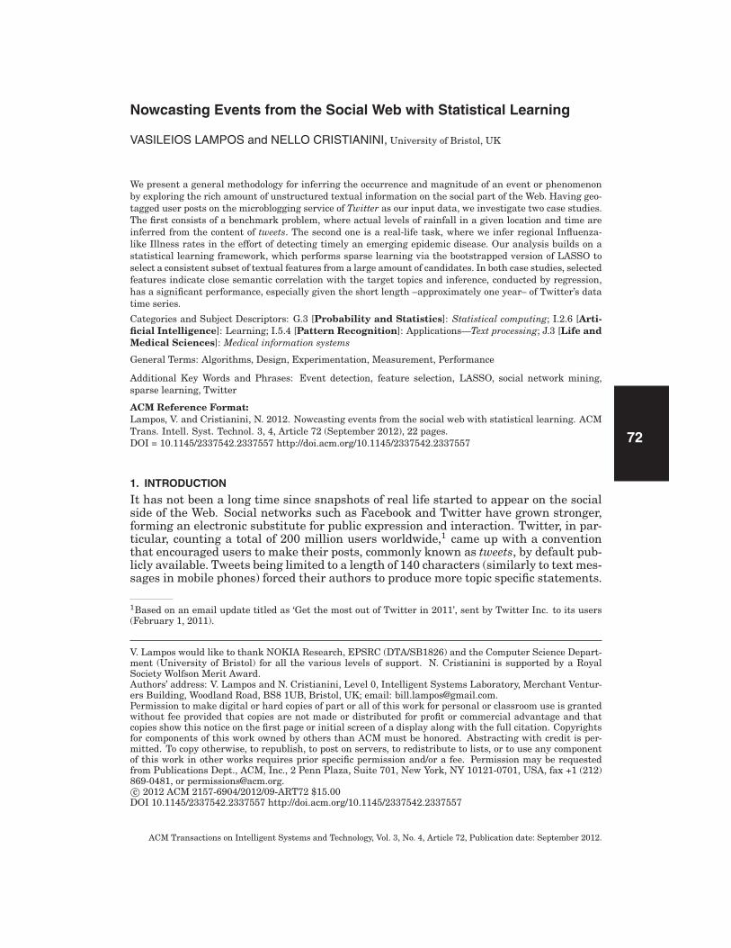
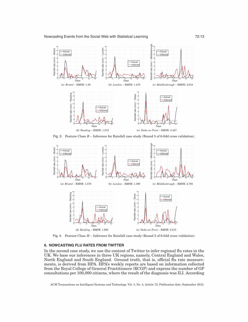
Fig. 2. Feature Class U – Inference for Rainfall case study (Round 5 of 6-fold cross validation).

formed by the exact union of the ones in classes U and B, but take different weights(Table V and Figure 1).

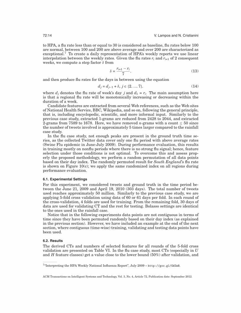
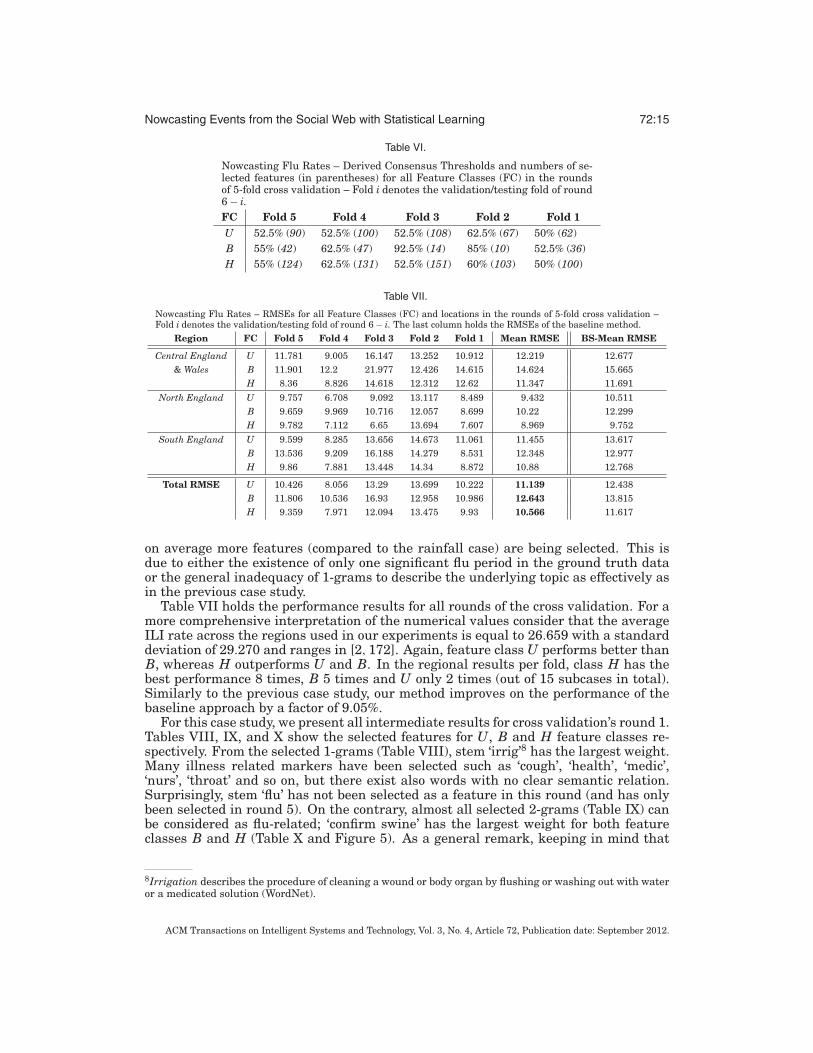
Inference results per location for cross validation’s round 5 are presented inFigures 2, 3, and 4 for U, B, and H feature classes respectively. Overall, inferencesfollow the pattern of actual rain; for feature class B, we see that inferences in someoccasions appear to have a positive lower bound (see Figure 3(e)) that is actually thepositive bias term of OLS regression appearing when the selected markers have zerofrequencies in the daily Twitter corpus of a location. As mentioned before this problemis resolved in H since it is very unlikely for 1-grams to also have a zero frequency.Results for class H depicted in Figures 4(a) (Bristol), 4(b) (London) and 4(d) (Reading)demonstrate a good fit with the target signal.



Fig. 3. Feature Class B – Inference for Rainfall case study (Round 5 of 6-fold cross validation).

Fig. 4. Feature Class H – Inference for Rainfall case study (Round 5 of 6-fold cross validation).

6. NOWCASTING FLU RATES FROM TWITTER

In the second case study, we use the content of Twitter to infer regional flu rates in theUK. We base our inferences in three UK regions, namely, Central England and Wales,North England and South England. Ground truth, that is, official flu rate measure-ments, is derived from HPA. HPA’s weekly reports are based on information collectedfrom the Royal College of General Practitioners (RCGP) and express the number of GPconsultations per 100,000 citizens, where the result of the diagnosis was ILI. According



to HPA, a flu rate less than or equal to 30 is considered as baseline, flu rates below 100are normal, between 100 and 200 are above average and over 200 are characterized asexceptional.7 To create a daily representation of HPA’s weekly reports we use linearinterpolation between the weekly rates. Given the flu rates ri and ri+1 of 2 consequentweeks, we compute a step factor δ from

δ =ri+1 − ri

7, (13)

and then produce flu rates for the days in between using the equation

dj = dj−1 + δ, j ∈ {2, ..., 7}, (14)

where dj denotes the flu rate of week’s day j and d1 = ri. The main assumption hereis that a regional flu rate will be monotonically increasing or decreasing within theduration of a week.

Candidate features are extracted from several Web references, such as the Web sitesof National Health Service, BBC, Wikipedia, and so on, following the general principle,that is, including encyclopedic, scientific, and more informal input. Similarly to theprevious case study, extracted 1-grams are reduced from 2428 to 2044, and extracted2-grams from 7589 to 1678. Here, we have removed n-grams with a count ≤ 50 sincethe number of tweets involved is approximately 5 times larger compared to the rainfallcase study.

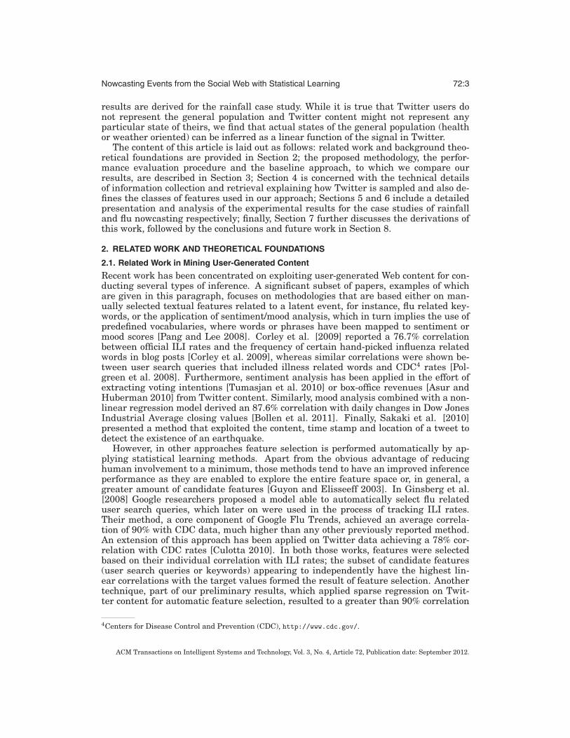
In the flu case study, not enough peaks are present in the ground truth time se-ries, as the collected Twitter data cover only one flu period with above average rates(Swine Flu epidemic in June-July 2009). During performance evaluation, this resultsin training mostly on nonflu periods where there is no strong flu signal; hence, featureselection under those conditions is not optimal. To overcome this and assess prop-erly the proposed methodology, we perform a random permutation of all data pointsbased on their day index. The randomly permuted result for South England’s flu rateis shown on Figure 10(c); we apply the same randomized index on all regions duringperformance evaluation.

6.1. Experimental Settings

For this experiment, we considered tweets and ground truth in the time period be-tween the June 21, 2009 and April 19, 2010 (303 days). The total number of tweetsused reaches approximately 50 million. Similarly to the previous case study, we areapplying 5-fold cross validation using data of 60 or 61 days per fold. In each round ofthe cross-validation, 4 folds are used for training. From the remaining fold, 30 days ofdata are used for validating CT and the rest for testing. Bolasso settings are identicalto the ones used in the rainfall case.

Notice that in the following experiments data points are not contiguous in terms oftime since they have been permuted randomly based on their day index (as explainedin the previous section). However, we have included an example at the end of the nextsection, where contiguous (time-wise) training, validating and testing data points havebeen used.

6.2. Results

The derived CTs and numbers of selected features for all rounds of the 5-fold crossvalidation are presented on Table VI. In the flu case study, most CTs (especially in Uand H feature classes) get a value close to the lower bound (50%) after validation, and

7“Interpreting the HPA Weekly National Influenza Report”, July 2009 – http://goo.gl/GWZmB.



Table VI.

Nowcasting Flu Rates – Derived Consensus Thresholds and numbers of se-lected features (in parentheses) for all Feature Classes (FC) in the roundsof 5-fold cross validation – Fold i denotes the validation/testing fold of round6 − i.FC Fold 5 Fold 4 Fold 3 Fold 2 Fold 1U 52.5% (90) 52.5% (100) 52.5% (108) 62.5% (67) 50% (62)B 55% (42) 62.5% (47) 92.5% (14) 85% (10) 52.5% (36)H 55% (124) 62.5% (131) 52.5% (151) 60% (103) 50% (100)

Table VII.

Nowcasting Flu Rates – RMSEs for all Feature Classes (FC) and locations in the rounds of 5-fold cross validation –Fold i denotes the validation/testing fold of round 6 − i. The last column holds the RMSEs of the baseline method.

Region FC Fold 5 Fold 4 Fold 3 Fold 2 Fold 1 Mean RMSE BS-Mean RMSE

Central England U 11.781 9.005 16.147 13.252 10.912 12.219 12.677& Wales B 11.901 12.2 21.977 12.426 14.615 14.624 15.665

H 8.36 8.826 14.618 12.312 12.62 11.347 11.691

North England U 9.757 6.708 9.092 13.117 8.489 9.432 10.511B 9.659 9.969 10.716 12.057 8.699 10.22 12.299H 9.782 7.112 6.65 13.694 7.607 8.969 9.752

South England U 9.599 8.285 13.656 14.673 11.061 11.455 13.617B 13.536 9.209 16.188 14.279 8.531 12.348 12.977H 9.86 7.881 13.448 14.34 8.872 10.88 12.768

Total RMSE U 10.426 8.056 13.29 13.699 10.222 11.139 12.438B 11.806 10.536 16.93 12.958 10.986 12.643 13.815H 9.359 7.971 12.094 13.475 9.93 10.566 11.617

on average more features (compared to the rainfall case) are being selected. This isdue to either the existence of only one significant flu period in the ground truth dataor the general inadequacy of 1-grams to describe the underlying topic as effectively asin the previous case study.

Table VII holds the performance results for all rounds of the cross validation. For amore comprehensive interpretation of the numerical values consider that the averageILI rate across the regions used in our experiments is equal to 26.659 with a standarddeviation of 29.270 and ranges in [2, 172]. Again, feature class U performs better thanB, whereas H outperforms U and B. In the regional results per fold, class H has thebest performance 8 times, B 5 times and U only 2 times (out of 15 subcases in total).Similarly to the previous case study, our method improves on the performance of thebaseline approach by a factor of 9.05%.

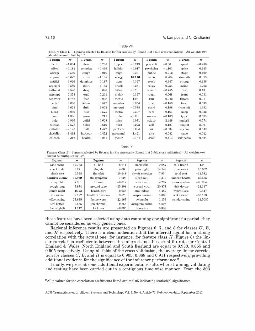
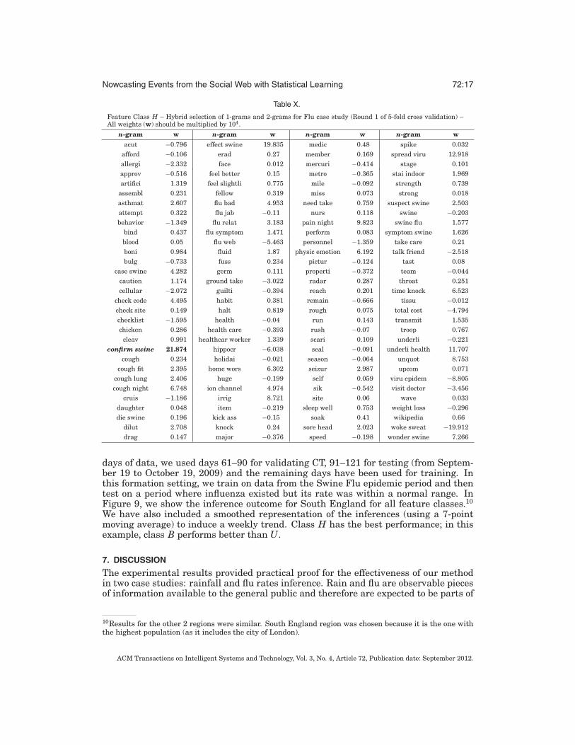
For this case study, we present all intermediate results for cross validation’s round 1.Tables VIII, IX, and X show the selected features for U, B and H feature classes re-spectively. From the selected 1-grams (Table VIII), stem ‘irrig’8 has the largest weight.Many illness related markers have been selected such as ‘cough’, ‘health’, ‘medic’,‘nurs’, ‘throat’ and so on, but there exist also words with no clear semantic relation.Surprisingly, stem ‘flu’ has not been selected as a feature in this round (and has onlybeen selected in round 5). On the contrary, almost all selected 2-grams (Table IX) canbe considered as flu-related; ‘confirm swine’ has the largest weight for both featureclasses B and H (Table X and Figure 5). As a general remark, keeping in mind that

8Irrigation describes the procedure of cleaning a wound or body organ by flushing or washing out with wateror a medicated solution (WordNet).



Table VIII.

Feature Class U – 1-grams selected by Bolasso for Flu case study (Round 1 of 5-fold cross validation) – All weights (w)should be multiplied by 104.

1-gram w 1-gram w 1-gram w 1-gram w 1-gram wacut −1.034 cleav 0.735 hippocr −6.249 properti −0.66 speed −0.286

afford −0.181 complex −0.499 holidai −0.017 psycholog −1.103 spike 0.145allergi −2.569 cough 0.216 huge −0.33 public 0.212 stage 0.109approv −0.672 cruis −1.105 irrig 10.116 radar 0.284 strength 0.873artifici 2.036 daughter 0.187 item −0.337 reach 0.247 strong 0.336

assembl 0.589 dilut 4.165 knock 0.261 reliev −0.254 swine 1.262asthmat 4.526 drag 0.098 lethal −0.73 remain −0.755 tast 0.13attempt 0.375 erad 0.201 major −0.367 rough 0.068 team −0.031behavior −1.747 face −0.008 medic 1.06 run 0.242 throat 0.07

better 0.066 fellow 0.542 member 0.354 rush −0.159 tissu 0.533bind 0.675 fluid 2.002 mercuri −0.588 scari 0.198 transmit 1.352blood 0.059 fuss 0.575 metro −0.397 seal −0.161 troop 0.532boni 1.308 germ 0.211 mile −0.081 season −0.103 typic 0.585bulg −0.966 guilti −0.608 miss 0.071 seizur 2.448 underli 0.774

caution 2.578 habit 0.619 nurs 0.223 self 0.127 unquot 8.901cellular −2.125 halt 1.472 perform 0.084 sik −0.634 upcom 0.642

checklist −1.494 harbour −0.472 personnel −1.451 site 0.042 wave 0.042chicken 0.317 health −0.241 pictur −0.134 soak 0.413 wikipedia 0.824

Table IX.

Feature Class B – 2-grams selected by Bolasso for Flu case study (Round 1 of 5-fold cross validation) – All weights (w)should be multiplied by 104.

2-gram w 2-gram w 2-gram w 2-gram wcase swine 12.783 flu bad 6.641 need take 0.887 talk friend −4.9check code 6.27 flu jab 4.66 pain night 14.149 time knock 10.002check site 0.568 flu relat 10.948 physic emotion 7.95 total cost −11.582

confirm swine 31.509 flu symptom 7.693 sleep well 1.319 underli health 25.535cough fit 7.381 flu web −8.017 sore head 4.297 virus epidem −28.204

cough lung 7.974 ground take −15.208 spread viru 20.871 visit doctor −12.327cough night 16.73 health care −0.636 stai indoor 5.482 weight loss −0.447die swine 9.722 healthcar worker 3.876 suspect swine 3.863 woke sweat −33.133

effect swine 27.675 home wors 22.167 swine flu 1.153 wonder swine 11.5085feel better 0.655 ion channel 9.755 symptom swine 5.895feel slightli 1.712 kick ass −0.335 take care 0.382

those features have been selected using data containing one significant flu period, theycannot be considered as very generic ones.

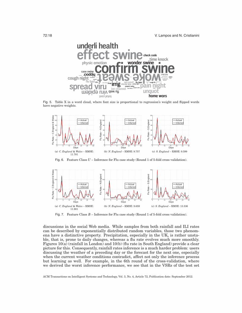
Regional inference results are presented on Figures 6, 7, and 8 for classes U, B,and H respectively. There is a clear indication that the inferred signal has a strongcorrelation with the actual one; for instance, for feature class H (Figure 8) the lin-ear correlation coefficients between the inferred and the actual flu rate for CentralEngland & Wales, North England and South England are equal to 0.933, 0.855 and0.905 respectively. Using all folds of the cross validation, the average linear correla-tion for classes U, B, and H is equal to 0.905, 0.868 and 0.911 respectively, providingadditional evidence for the significance of the inference performance.9

Finally, we present some additional experimental results where training, validatingand testing have been carried out in a contiguous time wise manner. From the 303

9All p-values for the correlation coefficients listed are � 0.05 indicating statistical significance.



Table X.

Feature Class H – Hybrid selection of 1-grams and 2-grams for Flu case study (Round 1 of 5-fold cross validation) –All weights (w) should be multiplied by 104.

n-gram w n-gram w n-gram w n-gram wacut −0.796 effect swine 19.835 medic 0.48 spike 0.032

afford −0.106 erad 0.27 member 0.169 spread viru 12.918allergi −2.332 face 0.012 mercuri −0.414 stage 0.101approv −0.516 feel better 0.15 metro −0.365 stai indoor 1.969artifici 1.319 feel slightli 0.775 mile −0.092 strength 0.739

assembl 0.231 fellow 0.319 miss 0.073 strong 0.018asthmat 2.607 flu bad 4.953 need take 0.759 suspect swine 2.503attempt 0.322 flu jab −0.11 nurs 0.118 swine −0.203behavior −1.349 flu relat 3.183 pain night 9.823 swine flu 1.577

bind 0.437 flu symptom 1.471 perform 0.083 symptom swine 1.626blood 0.05 flu web −5.463 personnel −1.359 take care 0.21boni 0.984 fluid 1.87 physic emotion 6.192 talk friend −2.518bulg −0.733 fuss 0.234 pictur −0.124 tast 0.08

case swine 4.282 germ 0.111 properti −0.372 team −0.044caution 1.174 ground take −3.022 radar 0.287 throat 0.251cellular −2.072 guilti −0.394 reach 0.201 time knock 6.523

check code 4.495 habit 0.381 remain −0.666 tissu −0.012check site 0.149 halt 0.819 rough 0.075 total cost −4.794checklist −1.595 health −0.04 run 0.143 transmit 1.535chicken 0.286 health care −0.393 rush −0.07 troop 0.767

cleav 0.991 healthcar worker 1.339 scari 0.109 underli −0.221confirm swine 21.874 hippocr −6.038 seal −0.091 underli health 11.707

cough 0.234 holidai −0.021 season −0.064 unquot 8.753cough fit 2.395 home wors 6.302 seizur 2.987 upcom 0.071

cough lung 2.406 huge −0.199 self 0.059 viru epidem −8.805cough night 6.748 ion channel 4.974 sik −0.542 visit doctor −3.456

cruis −1.186 irrig 8.721 site 0.06 wave 0.033daughter 0.048 item −0.219 sleep well 0.753 weight loss −0.296die swine 0.196 kick ass −0.15 soak 0.41 wikipedia 0.66

dilut 2.708 knock 0.24 sore head 2.023 woke sweat −19.912drag 0.147 major −0.376 speed −0.198 wonder swine 7.266

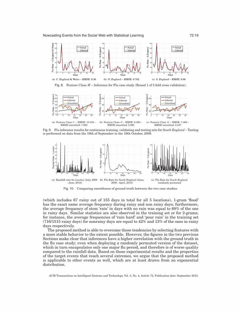
days of data, we used days 61–90 for validating CT, 91–121 for testing (from Septem-ber 19 to October 19, 2009) and the remaining days have been used for training. Inthis formation setting, we train on data from the Swine Flu epidemic period and thentest on a period where influenza existed but its rate was within a normal range. InFigure 9, we show the inference outcome for South England for all feature classes.10

We have also included a smoothed representation of the inferences (using a 7-pointmoving average) to induce a weekly trend. Class H has the best performance; in thisexample, class B performs better than U.

7. DISCUSSION

The experimental results provided practical proof for the effectiveness of our methodin two case studies: rainfall and flu rates inference. Rain and flu are observable piecesof information available to the general public and therefore are expected to be parts of

10Results for the other 2 regions were similar. South England region was chosen because it is the one withthe highest population (as it includes the city of London).



Fig. 5. Table X in a word cloud, where font size is proportional to regression’s weight and flipped wordshave negative weights.

Fig. 6. Feature Class U – Inference for Flu case study (Round 1 of 5-fold cross validation).

Fig. 7. Feature Class B – Inference for Flu case study (Round 1 of 5-fold cross validation).

discussions in the social Web media. While samples from both rainfall and ILI ratescan be described by exponentially distributed random variables, those two phenom-ena have a distinctive property. Precipitation, especially in the UK, is rather unsta-ble, that is, prone to daily changes, whereas a flu rate evolves much more smoothly.Figures 10(a) (rainfall in London) and 10(b) (flu rate in South England) provide a clearpicture for this. Consequently, rainfall rates inference is a much harder problem: usersdiscussing the weather of a preceding day or the forecast for the next one, especiallywhen the current weather conditions contradict, affect not only the inference processbut learning as well. For example, in the 6th round of the cross-validation, wherewe derived the worst inference performance, we see that in the VSRs of the test set



Fig. 8. Feature Class H – Inference for Flu case study (Round 1 of 5-fold cross validation).

Fig. 9. Flu inference results for continuous training, validating and testing sets for South England – Testingis performed on data from the 19th of September to the 19th October, 2009.

Fig. 10. Comparing smoothness of ground truth between the two case studies.

(which includes 67 rainy out of 155 days in total for all 5 locations), 1-gram ‘flood’has the exact same average frequency during rainy and non rainy days; furthermore,the average frequency of stem ‘rain’ in days with no rain was equal to 68% of the onein rainy days. Similar statistics are also observed in the training set or for 2-grams;for instance, the average frequencies of ‘rain hard’ and ‘pour rain’ in the training set(716/1515 rainy days) for nonrainy days are equal to 42% and 13% of the ones in rainydays respectively.

The proposed method is able to overcome those tendencies by selecting features witha more stable behavior to the extent possible. However, the figures in the two previousSections make clear that inferences have a higher correlation with the ground truth inthe flu case study; even when deploying a randomly permuted version of the dataset,which in turn encapsulates only one major flu period, and therefore is of worse qualitycompared to the rainfall data. Based on those experimental results and the propertiesof the target events that reach several extremes, we argue that the proposed methodis applicable to other events as well, which are at least drawn from an exponentialdistribution.



Another important point in this methodology regards the feature extraction ap-proach. A mainstream information retrieval technique implies the formation of a vo-cabulary index from the entire corpus [Manning et al. 2008]. Instead, we have chosento form a more focused and restricted in numbers set of candidate features from onlinereferences related with the target event, a choice justified by LASSO’s risk bound (seeEquation (10)). The short time span of our data limits the amount of training samples,and therefore directs us in the choice of reducing the number of the candidate featuresto minimize the risk error and avoid overfitting. Indeed, in the flu case study, whereonly a small variation in the ILI rates is observed, when we formed an index fromthe entire Twitter corpus, the method tended to select non-illness-related features aswell. Some of those features, for example, were describing a popular movie released inJuly 2009, the same period with the peak in the flu rates signal. By having fewer andslightly more focused on the target event’s domain candidates, we constrain the di-mensionality over training samples ratio and this issue is resolved. Nevertheless, thesize of 1-gram vocabularies in both case studies was not small (approx. 2400 words)and 99% of the daily tweets for each location or region contained at least one candidatefeature. However, for 2-grams this proportion was reduced to 1.5% and 3% for rainfalland flu rates case studies respectively, meaning that this class of features required amuch higher number of tweets in order to properly contribute.

The experimental process made also clear that a manual selection of very obviouskeywords that logically describe a topic, such as ‘flu’ or ‘rain’, might not be optimal es-pecially when using 1-grams; more rare words (‘puddl’ or ‘irrig’) exhibited more stableindications about the target events’ magnitude. Finally, it is important to note how CToperates as an additional layer in the feature selection process facilitating the adapta-tion on the special characteristics of each dataset. CT’s validation showed that a blindapplication of strict bolasso (CT = 1) would not have performed as good as the relaxedversion we applied; only once in 22 validation sets the optimal value for CT was setequal to 1.

8. CONCLUSIONS AND FUTURE WORK

We have presented a supervised learning framework for nowcasting events by ex-ploiting unstructured textual information published on the social Web. The proposedmethodology is able to turn geo-tagged user posts on the microblogging service ofTwitter to topic-specific geolocated signals by selecting textual features that capturesemantic notions of the inference target. Sparse learning via a soft version of Bolasso,the bootstrapped LASSO L1-norm regulariser, performs a consistent feature selection,which increases the inference performance approx. by a factor of 10% compared topreviously proposed methods [Culotta 2010; Ginsberg et al. 2008].

We have displayed results drawn from two case studies, that is, the benchmarkproblem of inferring rainfall rates and the real-life task of detecting the diffusion ofInfluenza-like Illness from tweets. In both case studies, the majority of selected fea-tures was directly related with the target topic and inference performance has beensignificant; for instance, for the important task of nowcasting influenza, inferred flurates reached an average correlation of 91.11% with the actual ones. As expected, se-lected 2-grams showed a better semantic connection with the target topics. However,during inference they did not perform as well as 1-grams. Combining both featureclasses into a hybrid approach resulted in an overall better performance.

Future work could be focused on improving various subtasks in our methodology.Feature extraction can become more sophisticated by identifying self diagnosticstatements in the corpus (e.g., “I got soaked today” or “I have a headache”) or by in-corporating entities (gender, names, brands, etc.). Similarly to other work (mentioned



in Section 2), using sentiment or mood analysis on the text can offer an additional di-mension of input information. Exploiting the temporal behavior of an event combinedwith more sophisticated inference techniques able to model non linearities or even agenerative approach, could also improve the inference performance as well as provideinteresting insights (e.g., the identification of latent variables that influence theinference process). Finally, on a conceptual basis, the detection of multivariate signals,where target variables may be interdependent (e.g., electoral voting intentions), couldform an interesting task for future research.

ACKNOWLEDGMENTS

The authors would like to thank Twitter Inc. and HPA for making their data publicly accessible, PASCAL2Network for the continuous support, and Tijl De Bie for providing feedback in early stages of this work. Weare also grateful to the anonymous reviewers for their constructive feedback.

REFERENCESASUR, S. AND HUBERMAN, B. A. 2010. Predicting the future with social media. In Proceedings of the

IEEE/WIC/ACM International Conference on Web Intelligence and Intelligent Agent Technology. IEEE,492–499.

BACH, F. R. 2008. Bolasso: Model consistent Lasso estimation through the bootstrap. In Proceedings of the25th International Conference on Machine Learning. 33–40.

BARTLETT, P. L., MENDELSON, S., AND NEEMAN, J. 2009. l1-regularized linear regression: Persistence andoracle inequalities. Tech. rep., UC-Berkeley.

BOLLEN, J., MAO, H., AND ZENG, X. 2011. Twitter mood predicts the stock market. J. Comput. Sci.BREIMAN, L. 1996. Bagging predictors. Mach. Learn. 24, 2, 123–140.CORLEY, C. D., MIKLER, A. R., SINGH, K. P., AND COOK, D. J. 2009. Monitoring influenza trends through

mining social media. In Proceedings of the International Conference on Bioinformatics and Computa-tional Biology. 340–346.

CULOTTA, A. 2010. Towards detecting influenza epidemics by analyzing Twitter messages. In Proceedingsof the KDD Workshop on Social Media Analytics.

EFRON, B. 1979. Bootstrap methods: Another look at the jackknife. Ann. Statist. 7, 1, 1–26.EFRON, B. AND TIBSHIRANI, R. J. 1993. An Introduction to the Bootstrap. Chapman & Hall.EFRON, B., HASTIE, T., JOHNSTONE, I., AND TIBSHIRANI, R. 2004. Least angle regression. Ann. Statist.

32, 2, 407–451.GINSBERG, J., MOHEBBI, M. H., PATEL, R. S., BRAMMER, L., SMOLINSKI, M. S., AND BRILLIANT, L. 2008.

Detecting influenza epidemics using search engine query data. Nature 457, 7232, 1012–1014.GUYON, I. AND ELISSEEFF, A. 2003. An introduction to variable and feature selection. J. Mach. Learn.

Resear. 3, 7–8, 1157–1182.JENKINS, G. J., PERRY, M. C., AND PRIOR, M. J. 2008. The Climate of the United Kingdom and Recent

Trends. Met Office, Hadley Centre, Exeter, UK.LAMPOS, V. AND CRISTIANINI, N. 2010. Tracking the flu pandemic by monitoring the Social Web. In Pro-

ceedings of the 2nd IAPR Workshop on Cognitive Information Processing. IEEE Press, 411–416.LAMPOS, V., DE BIE, T., AND CRISTIANINI, N. 2010. Flu detector—Tracking epidemics on Twitter. In Pro-

ceedings of the European Conference on Machine Learning and Principles and Practice of KnowledgeDiscovery in Databases. Springer, 599–602.

LV, J. AND FAN, Y. 2009. A unified approach to model selection and sparse recovery using regularized leastsquares. Ann. Statist. 37, 6A, 3498–3528.

MANNING, C. D., RAGHAVAN, P., AND SCHUTZE, H. 2008. Introduction to Information Retrieval. CambridgeUniversity Press.

PANG, B. AND LEE, L. 2008. Opinion mining and sentiment analysis. Found. Trends Inf. Retriev. 2, 1–2,1–135.

POLGREEN, P. M., CHEN, Y., PENNOCK, D. M., NELSON, F. D., AND WEINSTEIN, R. A. 2008. Using internetsearches for influenza surveillance. Clinical Infectious Diseases 47, 11, 1443–1448.

PORTER, M. F. 1980. An algorithm for suffix stripping. Program 14, 3, 130–137.



SAKAKI, T., OKAZAKI, M., AND MATSUO, Y. 2010. Earthquake shakes Twitter users: Real-time event detec-tion by social sensors. In Proceedings of the 19th International Conference on World Wide Web. 851–860.

TIBSHIRANI, R. 1996. Regression shrinkage and selection via the lasso. J. Royal Statist. Soc. Series B(Methodological) 58, 1, 267–288.

TUMASJAN, A., SPRENGER, T. O., SANDNER, P. G., AND WELPE, I. M. 2010. Predicting elections withTwitter: What 140 characters reveal about political sentiment. In Proceedings of the International AAAIConference on Weblogs and Social Media. 178–185.

ZHAO, P. AND YU, B. 2006. On model selection consistency of Lasso. J. Mach. Learn. Resear. 7, 11,2541–2563.

Received April 2011; revised August 2011; accepted September 2011


Documents

Nowcasting Events from the Social Web with … · Nowcasting Events from the Social Web with Statistical Learning ... We present a general methodology for inferring the ... Nowcasting