a dual algorithm for approximating pareto sets in convex multi - KTH

A DUAL ALGORITHM FOR APPROXIMATING PARETO

SETS IN CONVEX MULTI-CRITERIA OPTIMIZATION

Rasmus BOKRANTZ∗†‡ and Anders FORSGREN†

Technical Report TRITA-MAT-2011-OS3Department of MathematicsRoyal Institute of Technology

February 2011

Abstract

We consider the problem of approximating the Pareto set of convex multi-criteria optimization problems by a discrete set of points and their convex com-binations. Finding the scalarization parameters that maximize the improve-ment in bound on the approximation error when generating a single Paretooptimal solution is a nonconvex optimization problem. This problem is solv-able by enumerative techniques, but at a cost that increases exponentially withthe number of objectives. The goal of this paper is to present a practical al-gorithm for solving the Pareto set approximation problem in presence of upto about ten conflicting objectives, motivated by application to radiation ther-apy optimization. To this end, an enumerative scheme is proposed that is ina sense dual to the algorithms in the literature. The proposed technique re-tains the quality of output of the best previous algorithm while solving fewersubproblems. A further improvement is provided by a procedure for discardingsubproblems based on reusing information from previous solves. The combinedeffect of the proposed enhancements is empirically demonstrated to reduce thecomputational expense of solving the Pareto surface approximation problem byorders of magnitude.

1. Introduction

Multi-criteria optimization (MCO) deals with optimization problems involving mul-tiple mutually conflicting objectives, see, e.g., the monographs [5, 20, 36]. For suchproblems in general, there is no feasible solution that is optimal with respect to allobjectives simultaneously. Instead, a well-balanced trade-off between objectives issought within the Pareto optimal set: the set encompassed by the feasible solutionssuch that an improvement in one objective can only be achieved through a sacrificein another. One approach to identifying a suitable trade-off between objectives is topre-compute a finite number of solutions without human interaction, and then takethese as input to a navigation tool that allows feasible trade-offs to be evaluated inreal-time by forming convex combinations between discrete solutions, see [16,22,38].

∗E-mail: [email protected]†Optimization and Systems Theory, Department of Mathematics, Royal Institute of Technology

(KTH), SE-100 44 Stockholm, Sweden.‡RaySearch Laboratories, Sveavagen 25, SE-111 34 Stockholm, Sweden.

2 A dual algorithm for approximating Pareto sets

This technique is particularly suited for large-scale problems where a single opti-mization run is costly, and by design, imposes a restriction to problem formulationswith convex constraints.

We are particularly interested in application of the described technique to treat-ment planning for intensity modulated radiation therapy (IMRT). There is a richliterature of methods that recognize IMRT planning as an MCO problem, see,e.g., [9, 12–14, 31, 32]. Clinical evaluations have demonstrated that such methodshave the potential of improving both manual planning time and treatment qual-ity [15, 26, 51]. In view of this application, we limit ourselves to generating Paretooptimal points by replacing the vector-valued objective function of the initial prob-lem with a convex combination of its components. This weighting method is exten-sively used throughout the field of MCO [34] and is the de facto standard method forIMRT optimization [1,28]. We further limit ourselves to consider convex objectives,so that the Pareto optimal set forms a connected surface in the boundary of a convexset [44]. Convex criteria that are commonly used in IMRT planning together withnonconvex criteria that can be reformulated into convex such are surveyed in [44].

Within this context, we consider the problem of generating a discrete set ofPareto optimal solutions so that the lower boundary of their convex hull provides arepresentative approximation of the Pareto surface. We focus on so-called sandwichalgorithms, which maintain inner and outer approximations of the Pareto surface,see [7,23,45] for algorithms in the plane and [13,30,42,48] for algorithms in generaldimensions. The inner and outer approximations are used to steer generation ofnew points towards parts of the Pareto surface that currently lack accurate rep-resentation, and to provide an approximation guarantee for the current discreterepresentation.

The computational expense of a sandwich algorithm increases exponentially withthe number of objectives. This behavior is fundamentally due to what is called “thecurse of dimensionality”: in direct sampling of a distribution of data, the number ofsamples required to maintain a given level of accuracy increases exponentially withthe number of variables [2]. As a consequence, application of sandwich algorithmsto problems with more than six objectives has, to the best of our knowledge, previ-ously not been reported. The number of objectives commonly encountered in IMRTplanning, on the other hand, range up to about ten [11, 49]. Current practice forhigh-dimensional cases is to sample weights uniformly at random. This technique iswell-known to be inadequate for generating an even distribution of points from allparts of the Pareto surface [17].

Motivated by these shortcomings, we develop methods for making sandwich al-gorithms tractable to a wider range of problem formulations. We devote particularattention to the mathematical programming and computational geometry aspectsof this problem. For many problems within these two fields, primal and dual for-mulations have equivalent complexity in the general case. However, as noted byBremner [6, p. 2] with respect to polytope duality: “for a particular class of poly-topes and a fixed algorithm, one transformation may be much easier than its dual.”Arguing that this is the case for sandwich algorithms, we give an algorithm that in asense is dual to algorithms in the literature. Our main contribution is a scheme that

2. Preliminaries 3

retains the quality of output of the best previous algorithm while achieving a morebenign ratio between computational effort and problem dimension. The presentedalgorithm also generalizes sandwich algorithms to be compatible with cone-basedpreference models, see e.g., [21,27,37]. For the IMRT application, such models haveproven useful for excluding parts of the Pareto surface that are known a priori tonot be of interest, see [47].

2. Preliminaries

2.1. Notation and terminology

We denote by e the vector of ones with dimension defined by the context. Vectorinequalities are to be understood componentwise. We treat sets of points and ma-trices interchangeably when convenient; the rows of the matrix are the elements ofthe corresponding set. The shorthand (·)+ is used to denote max{·, 0}. We denotethe optimal value of an optimization problem P by optval(P ). For a function f andsubset S of its domain, we denote by f(S) the image {f(s) : s ∈ S}. For a set S,we denote by conv(S) its convex hull. For two sets S1 and S2, we denote by S1+S2

their Minkowski sum. Minkowski addition between a set S and a singleton set {s} isdenoted by s+S. A hyperplane

{

z : aT z = b}

with nonzero normal a and offset b isdenoted by H(a, b). With each hyperplane, we associate a closed positive, a closednegative, an open positive and an open negative halfspace, defined by substitutingrespectively “≥,” “≤,” “>,” and “<” for the equality in the hyperplane equation.The intersection of a finite number of closed halfspaces is called a polyhedron. Aclosed and bounded polyhedron is called a polytope. The k-dimensional intersectionbetween a polyhedron and one of its supporting hyperplanes is called a k-face. A0-face is called a vertex, a 1-face an edge, an (n − 2)-face a ridge, and an (n − 1)-face a facet. Unless the contrary is stated, a normal vector to a polyhedral face isassumed to be oriented inwards.

2.2. Problem formulation

The algorithm to be described applies to a multi-objective optimization problemson the form

(MOP)minimize

x(f1(x), . . . , fn(x))

T

subject to x ∈ X = {x : c(x) ≤ 0} ,(2.1)

involving n ≥ 2 objective functions fi to be minimized over a feasible regionX ⊆ IRm

defined by a vector c of constraint functions. We denote by f the n-vector ofobjective functions and by Z the image of the feasible region under the objectivefunction mapping, i.e., Z = f(X). We refer to the m-dimensional space of whichX is a subset as the decision space and to the n-dimensional space of which Z is asubset as the objective space. Throughout, the feasible region X is assumed to benonempty and the functions f and c to be convex and bounded on X. The feasibleregion is a convex set by virtue of that all sublevel sets of convex functions areconvex. Since f and X are both convex, MOP is a convex optimization problem.


2.3. Notion of optimality

The solution set to MOP is the set of nondominated feasible points. Dominancerelations between points in objective space are defined with respect to the partialorder induced by some ordering cone C which we require to be closed, pointed(i.e., 0 ∈ C), salient (i.e., C ∩ −C ⊆ {0}), convex, and containing IRn

+.

Definition 2.1. (Nondominance) Let x∗ be feasible to MOP. Then, x∗ is non-dominated if there exists no x in X such that f(x∗) ∈ f(x) + C \ {0}.

In order to distinguish between the decision space and the objective space moreeasily, we refer to a nondominated solution x∗ as efficient whereas the correspondingobjective vector f(x∗) is called Pareto optimal. We refer to the set of all efficientsolutions as the efficient set and to the set of all Pareto optimal objective vectors asthe Pareto set.

We restrict ourselves to consider polyhedral ordering cones generated by somematrix Q, i.e., C = {Qµ : µ ≥ 0}. Instead of specifying Q directly, we prefer todefine the set of admissible trade-off rates between objectives and let this set bethe dual cone C∗ = {z : yT z ≥ 0 ∀y ∈ C} to C. Let T be the symmetric n × nmatrix with unit diagonal and nonnegative off-diagonal elements tij such that thereciprocal of tij is the maximum acceptable increase in fi for a unit decrease in fj .Then, C∗ is the polyhedral cone generated by T , and C the dual cone to C∗, i.e.,C = {z : Tz ≥ 0}, here using that C = C∗∗ by convexity and closedness of C [50, p.53]. By construction, C∗ ⊆ IRn

+, so that IRn+ ⊆ C [50, p. 56]. Taking T and Q to

be the identity matrix, so that C = C∗ = IRn+, gives dominance in the conventional

Pareto sense.

2.4. The weighting method

A Pareto optimal solution can be computed by introducing an n-vector w of weightssuch that w ∈ C∗ and solving the scalar-valued optimization problem

(SUM(w))minimize

x

∑ni=1wifi(x)

subject to x ∈ X.(2.2)

This is a convex optimization problem by virtue of that C∗ ⊆ IRn+ and since nonneg-

ative linear combinations preserve convexity. The vector w is throughout assumedto be normalized so that eTw = 1.

Problems MOP and SUM(w) are related as follows. If a point x∗ is optimalto SUM(w) for some w in C∗ such that w > 0, then x∗ is efficient to MOP [36,Thm. 3.1.2]. For any x∗ that is efficient to MOP, there exists w in C∗ such thatx∗ is optimal to SUM(w) [36, Thm. 3.1.4]. The second of these results relies onconvexity of MOP. As an immediate consequence, if x∗ is optimal to SUM(w) forsome w in C∗, the hyperplane H(w, f(x∗)) supports the feasible objective space Zat f(x∗). To see this, observe that f(x∗) ∈ Z∩H(w, f(x∗)) and that the intersectionbetween Z and the open negative halfspace associated with H(w, f(x∗)) is empty,or otherwise x∗ would not be optimal to SUM(w). Finding any point on the Paretosurface thus reduces to solving SUM(w) with w normal to the Pareto surface at thesought point.

3. The sandwich algorithm 5

3. The sandwich algorithm

3.1. The algorithmic idea

A generic sandwich algorithm is given in Algorithm 3.1. The goal of this algorithm isto generate a set of points such that their convex hull constitutes an approximationof the efficient set with approximation error below some tolerance ε > 0, in as fewsolves as possible. The algorithm avoids assessing the quality of the approximationof the efficient set in the typically high-dimensional decision space by a mapping tothe objective space and evaluating the resulting image with respect to the Paretosurface. An upper bound on the approximation error is calculated as the distancebetween polyhedral inner and outer approximations of the Pareto surface. Theweighting vector in the next weighted-sum problem to be solved is taken to benormal to the inner approximation at the point where the upper bound is attained.This choice corresponds to the greedy strategy of maximizing the decrease in boundon the approximation error at each iteration.

The first two steps in Algorithm 3.1 serve to normalize the range of each objectivefunction, as to avoid bias towards objectives with a large order of magnitude. Wehere use the pragmatic approach of normalizing each objective function with respectto its minimum and maximum objective value during the n initial solves of SUM(w).We refer to an iteration of the while loop in Algorithm 3.1 as an iteration of thesandwich algorithm.

Algorithm 3.1. The sandwich algorithm

for i = 1, . . . , n do solve SUM(ti) with respect to the ith extreme ray ti of C∗;

normalize f to [0, 1]n;solve SUM(w) with w = 1

ne;

construct inner and outer approximations Zin and Zout of the Pareto surface;while not converged do

compute an upper bound on the approximation error;if the upper bound is below ε then converged; break;solve SUM(w) with w normal to Zin where the upper bound is attained;update Zin and Zout;

end

3.2. Overview of previous general-dimensional sandwich algorithms

Three algorithms are of immediate interest with respect to the algorithm we propose:those of Solanki et al. [48], Craft et al. [13] and Rennen et al. [42], where the twolatter algorithms can be viewed as enhanced versions of the proceeding one(s). Anygeneral-dimensional sandwich algorithm must handle the fact that a vector normal


to the convex hull of a discrete set of Pareto optimal points can have negative com-ponents in dimension beyond two. Hence, if such a normal vector is used directlyas weighting vector w in solving SUM(w), this vector may not lie in C∗, and theresulting optimal solution may not be efficient to MOP. The algorithm of Solanki etal. handles this complication by introducing bounds on the allowed deviation fromthe Pareto surface. In the algorithm of Craft et al., a heuristic method is insteadused for transforming mixed normals into nonnegative such, as to make better useof each optimization run. The algorithm of Rennen et al. avoids mixed normalsaltogether by augmenting the convex hull representation of the inner approxima-tion through setwise summation with the nonnegative orthant. Any normal to theresulting polyhedron is nonnegative [42, Lemma 2]. In [42], the three algorithmsare empirically evaluated on a suite of test problems. This study indicates that thealgorithm of Rennen et al. generates well-distributed points on the Pareto surfaceand provide a corresponding rapid improvement in bound on the approximationerror, whereas this is generally not the case for the algorithms of Solanki et al. andCraft et al. Based on these findings, we use the algorithm of Rennen et al. as asingle benchmark to the algorithm proposed in this paper, both in the theoreticalexposition and the numerical experiments.

In the remainder of this section, we define polyhedral approximations of thePareto surface and a quality measure on a discrete representation of the Paretoset. These definitions generalize those of Rennen et al. to dominance induced by ageneral ordering cone. A novel approach for performing the steps encompassing aniteration of the sandwich algorithm is proposed in Section 4.

3.3. Polyhedral approximations

The key result that makes construction of polyhedral approximations of the Paretosurface possible is that the set Z+ = Z+C is a convex set whenever MOP is a convexproblem. This result is a generalization of the result that a function is convex ifand only if its epigraph is a convex set to the case of epigraphs induced by convexcones [40]. Other proofs of this result for the case C = IRn

+ can be found in [10,44].Convexity of Z+ implies that the convex hull of any discrete set of points in Z+ is aninner approximation of this set, and that the intersection of any set of closed positivehalfspaces associated with supporting hyperplanes to Z+ an outer approximation.In particular, polyhedral approximations of Z+ can be constructed as follows.

Definition 3.1. (Inner and outer approximations) Let D be a discrete set ofpoints that are efficient to MOP and optimal to SUM(w) with respect to some setW of weighting vectors in C∗. Then, Zin = {P Tλ + QTµ : λ, µ ≥ 0, eTλ = 1}where P = f(D) is an inner approximation of Z+, and Zout = {z : Wz ≥ r} wherer is the vector of pairwise scalar products between elements in P and W an outerapproximation of Z+, in the sense that Zin ⊆ Z+ ⊆ Zout.

Shrinking the hypervolume between Zin and Zout provide a means of approximatingthe Pareto surface with increased accuracy as this set must confine to the lowerboundary of Z+.

4. The vertex enumerative algorithm 7

3.4. Quantifying the approximation error

Quality measures of discrete representations of the Pareto set have been reviewedin [46]. The definition we give quantifies the coverage of the Pareto set in terms ofa relaxation of the nondomincance criterion.

Definition 3.2. (Approximation error) LetD be a discrete set of feasible pointsto MOP. Then, the approximation error of D is the minimum ε such that for anyefficient x∗, there exists x in conv(D) such that f(x∗) ∈ f(x) + (C − εe).

Unfortunately, explicit knowledge of the Pareto set is required to compute the abovedefined quantity. Since the entire Pareto set in general is not known, we will ex-clusively work with the upper bound on the approximation error provided by theminimum ε such that Zout ⊆ (Zin − εe). This upper bound is equivalent to theHausdorff distance

h(Zin, Zout) = maxz∈Zout

minz′∈Zin

d(z, z′),

taken with respect to the one-sided distance function

d(z, z′) = maxi∈{1,...,n}

(z′i − zi)+.

Computing h(Zin, Zout) requires solving the linear bilevel program

maximizez

minimizeη, λ, µ

η

subject to ηe ≥ P Tλ+QTµ− z,eTλ = 1,η, λ, µ ≥ 0,

(3.1)

subject to Wz ≥ r. (3.2)

Linear bilevel problems have been shown to be NP-hard and inapproximable withinany constant factor in polynomial time [18, Thm. 3.12]. Problems within this classmay be exactly solvable by enumerative techniques in moderate problem dimensions,see, e.g., [39], whereas finding the optimum to large-scale instances is in general nottractable.

4. The vertex enumerative algorithm

4.1. Solution by enumerating the vertices of the outer approximation

We propose to solve (3.1) by enumerating the extreme points of its feasible regionand solving a linear programming subproblem for each extreme point found. Theextreme points of the outer approximation are its finitely many vertices by virtue ofthat this set is polyhedral. Validity of the proposed method relies on the followingresults.

Proposition 4.1. At least one vertex of the outer approximation is an optimalsolution to (3.1).


Proof. The inner level linear program in (3.1) can be put on standard form byintroducing slack variables for each inequality constraint. Then, since the optimalvalue of a linear program on standard form is a convex, piecewise affine and contin-uous function of its right hand side coefficients [33, Lemma 1–2], problem (3.1) bya change of sign in the objective function amounts to minimizing a concave func-tion over a convex set. Since every global and local minimum value of a concavefunction is either attained at an extreme point of its feasible domain or the functionis unbounded from below on a feasible ray [43, Thm. 32.3], the proof reduces toshowing that the objective value of (3.1) is nonincreasing on any ray in Zout. Let zand p be vectors such that {z + αp : α ≥ 0} is a ray in Zout, i.e., z ∈ Zout, p 6= 0,and Wp ≥ 0. Let also (η, λ, µ) denote an optimal solution to the inner level linearprogram in (3.1) with respect to z. Since every row vector in W lies in C∗, wehave that p ∈ C, and therefore, there exists µ ≥ 0 such that p = Qµ. For such µ,(η, λ, µ + αµ) is feasible to the inner level linear program in (3.1) with respect toz + αp with objective value η. The objective value of (3.1) in any point on the rayis thus bounded from above by the objective value in the point z from which theray emanates, and the proof is complete.

As a direct consequence of this results, the optimal value of (3.1) is given bymaxv∈V optval(PLP(v)), where V denotes the set of vertices of the outer approxi-mation and where

minimizeη, λ, µ

η (4.1a)

(PLP(v)) subject to ηe ≥ P Tλ+QTµ− v, (4.1b)

eTλ = 1, (4.1c)

η, λ, µ ≥ 0. (4.1d)

We will for the moment postpone how to enumerate the vertices of Zout and insteaddiscuss some properties of this problem.

4.2. Identifying the next weighting vector

Having solved all instances of (4.1), we turn to identifying the weighting vector ofthe next weighted-sum problem that is to be solved. Similar lines of reasoning havepreviously been applied to a related problem in [10]. The linear programming dualto PLP(v) takes the form

maximizeπ, ρ

ρ− vTπ (4.2a)

(DLP(v)) subject to Pπ ≥ ρe, (4.2b)

Qπ ≥ 0, (4.2c)

eTπ ≤ 1, (4.2d)

π ≥ 0. (4.2e)

It is straightforward to verify that PLP(v) is feasible and its objective value boundedfrom below. Therefore, by linear programming duality, DLP(v) is feasible and its


objective value bounded from above. Moreover, for any primal-dual optimal solu-tion (η, λ, µ, π, ρ) to PLP(v) and DLP(v) associated with some v in V such thatoptval(PLP(v)) > 0, π lies in C∗ and is normal to the inner approximation aty = P Tλ+QTµ. This claim is made precise in Proposition 4.2. The next weightingvector is thus given by the vector of optimal dual variables π to the instance ofDLP(v) with maximum optimal value.

Proposition 4.2. Let (η, λ, µ, π, ρ) denote a primal-dual optimal solution to PLP(v)and DLP(v) defined by some vertex v in V such that η > 0. Then, H(π, ρ) is a sup-porting hyperplane to Zin at y = P Tλ+QTµ with normal vector π in C∗ \ {0}.

Proof. Feasibility and boundedness of PLP(v) and DLP(v) by strong duality forlinear programming imply that optval(PLP(v)) = optval(DLP(v)), or equivalently

η = ρ− vTπ. (4.3)

This result, the assumption that η > 0, (4.2b), and (4.2e) together imply thatπ 6= 0. The set H(π, ρ) thus forms a hyperplane in objective space with normalπ in C∗ \ {0} by feasibility with respect to (4.2c). To show that H(π, ρ) supportsZin at y, it remains to show that Zin is entirely contained in the closed positivehalfspace associated with H(π, ρ) and that y is contained in H(π, ρ). Take any y inZin parameterized by some µ and λ that are feasible to (4.1), i.e., y = P T λ+QT µ.Then,

πT y = πT (P T λ+QT µ) ≥ {(4.2c), (4.1d)} ≥ πTP T λ ≥

≥ {(4.2b)} ≥ ρλT e = {(4.1c)} = ρ,(4.4)

which yields the first part of the statement. Forming the scalar product between πand y gives that

πT y = πT (P Tλ+QTµ) ≤ {(4.1b)} ≤ πT (ηe+ v) ≤

≤ {(4.2d)} ≤ η + πT v = {(4.3)} = ρ.(4.5)

Inserting y in (4.4) gives that πT y ≥ ρ. Therefore, all inequalities in (4.5) are tight,so that y ∈ H(π, ρ).

4.3. Reducing the number of subproblems to be solved

The number of linear programming subproblems on the form (4.1) that needs to besolved to compute the optimal value of (3.1) can be reduced by upper-bounding theoptimal value of (4.1). Consider a sequence of solves of PLP(v) over v in V andlet β∗ denote the maximum optimal value obtained so far. Then, any vertex v inV that is optimal to (3.1) must satisfy optval(PLP(v)) ≥ β∗, and therefore, for anyvertex v in V and scalar β such that optval(PLP(v)) ≤ β ≤ β∗, the instance PLP(v)need not be solved. An upper bound on the optimal value of (4.1) is provided bythe following result.


Proposition 4.3. Let Zout = {z : Wz ≥ r} denote the outer approximation, V itsset of vertices and PLP(v) an instance of (4.1) defined by some v in V in an iterationof the sandwich algorithm, and let the corresponding notation with superscript “+”apply to the subsequent iteration. Then, for any v in V +, it holds that

optval(PLP+(v)) =

{

optval(PLP(v)) if v ∈ V +

maxv∈E optval(PLP(v)) otherwise,

where E is extreme point set of the unique edge of Zout that contains v.

Proof. First suppose that v ∈ V and let (η, λ, µ) be an optimal solution toPLP(v). Then, (η, (λT 0)T , µ) is a feasible solution to PLP+(v) with objectivevalue optval(PLP(v)). Hence, optval(PLP+(v)) ≤ optval(PLP(v)). Now supposethat v 6∈ V . Since v ∈ V +, the system W+v ≥ r+ is satisfied with equality inexactly n linearly independent rows. Similarly, v 6∈ V and Z+

out ⊆ Zout implythat the system Wv ≥ r is satisfied with equality in at most n − 1 linearly in-dependent rows. Then, since W+ is W augmented with one additional row, thissystem is satisfied with equality in exactly n − 1 linearly independent rows. Thepoint v is thus contained in an edge of Zout. By an argument analogous to thatin Proposition 4.1, the maximum optimal value of the inner level linear programin (3.1) taken over all points in this edge occurs at one of its extreme points, so thatoptval(PLP+(v)) ≤ maxv∈E optval(PLP(v)).

4.4. Enumerating the vertices of the outer approximation

We enumerate the vertices of the outer approximation by first representing this setas a polytope and then converting its halfspace representation to a vertex represen-tation. To perform the latter of these two steps, we use the fact that vertex enumer-ation is equivalent to a convex hull problem under polar duality between points andhyperplanes defined by a reciprocation H(a, b) 7→ (a1/b, . . . , an/b)

T about the unitsphere [41]. We first define a duality relation between polytopes and then outlinethe vertex enumerative scheme.

Definition 4.1. (Polytope duality) Let A be a polytope that contains the originin its strict interior. Then, the polytope A∗ = {z : yT z ≤ 1, ∀y ∈ A} is the polardual of A.

Polar duality defines a bijection between the facets of a polytope and the verticesof its dual. This correspondence is inclusion-reversing in the sense that two facetsthat incident on a common ridge are in bijection with two vertices contained in acommon edge [25, Thm. 3.4.4]. Polar duality is moreover a reflexive transformation,so that twice dualizing a polytope gives back the initial polytope [25, Thm. 3.4.3].

We use the above the theory to enumerate the vertices of the outer approximationby the following steps: (i) augment the outer approximation with n sufficiently largeupper bounds so that the resulting set is closed and bounded; (ii) identify a pointin the interior of the resulting primal polytope, e.g., the arithmetic mean of the


vertices of the inner approximation; (iii) translate the coordinate system so thatthis point is the origin; (iv) dualize the outwards oriented bounding hyperplanesof the primal polytope; (v) solve for the convex hull of the resulting points, thusobtaining a halfspace representation of the dual polytope; (vi) dualize the facet-inducing hyperplanes of the dual polytope (vii) translate the resulting points backinto the initial coordinate system; (viii) remove any point that satisfy any of theauxiliary upper bounds with equality. The resulting set of points form the verticesof the outer approximation.

4.5. Performing the polyhedral computations on-line

The problem that arises in step (v) of the procedure described in the above sectionis the so-called on-line convex hull problem: we are given points one point at atime and after receiving each point, we are to compute the convex hull of the pointsreceived so far. The variant of this problem in which all input points are known inadvance is called the off-line convex hull problem.

We solve the on-line convex hull problem by maintaining a graph representationof the current convex hull with facets as nodes and ridges between adjacent facets asedges. We make the mild assumption that the vertices of the dual polytope are innondegenerate position, i.e., no (n+1)-tuple of points lie in a common hyperplane.By this assumption, any facet of the dual polytope is an (n − 1)-simplex incidenton exactly n ridges, and dually, exactly n edges of the primal polytope are inci-dent on any common vertex [25]. Nondegeneracy can be simulated using standardperturbations techniques, see, e.g., [19, p. 185].

The facet graph is updated using a so-called beneath-and-beyond step, see,e.g., [19, 41]. In brief, one such step processes a new point by partitioning thefacets of the current convex hull into disjoint sets of visible and obscured facets.A facet is visible if it contains the new point in its associated open negative half-space. Obscured facets are reversibly defined. One visible facet is first identified.Remaining visible facets then found by depth-first search through adjacent visiblefacets, here using that the set of visible facets form a connected subgraph. A coneof new facets is created from the new point to all ridges on which one visible andone obscured facet are incident. The visible facets are finally deleted.

Efficiently identifying the first visible facet is non-trivial in the general on-lineversion of the convex hull problem. However, since the vertex v of the outer ap-proximation that in a given iteration was found to be most distant from the innerapproximation cannot be a vertex of the outer approximation in the subsequent it-eration, a visible facet is for our problem instance immediately available as the facetdual to v. With an on-line convex hull algorithm, p iterations of the sandwich al-gorithm requires p number of beneath-and-beyond steps. This should be contrastedto

∑pk=1 k = p(p+1)/2 steps with the straightforward solution of calling an off-line

algorithm in every iteration.

The upper-bounding technique of Section 4.3 can be incorporated with the de-scribed convex hull method as follows. With each facet of the dual polytope thatis dual to a vertex v of the outer approximation, we attach the current best upper


bound on optval(PLP(v)). This upper bound is updated whenever PLP(v) is solved.At the creation of a new facet, its upper bound is initialized as the maximum overupper bounds attached to any of the two facets incident on the ridge by which thenew facet is induced. Validity of this update rule follows from that the ridge isdual to an edge of the outer approximation defined as in Proposition 4.3 by theincidence-reversing property of polytope duality.

5. Comparison with the facet enumerative algorithm

5.1. Solution by enumerating the facets of the inner approximation

In the algorithm of Rennen et al., problem (3.1) is solved by enumerating the facet-inducing hyperplanes of the inner approximation. Let F denote the set of facet-inducing hyperplanes of Zin and take any hyperplane H(a, b) in F . Then, if λ andµ in (3.1) are restricted to values such that P Tλ + QTµ ∈ H(a, b), the optimalvalue function of the inner level linear program in (3.1) decomposes by algebraicmanipulations into (b−aT z)/(aT e). The optimal value of (3.1) can thus be obtainedby solving a linear program

(LP(a))minimize

zaT z

subject to Wz ≥ r,(5.1)

for each hyperplane H(a, b) in F and taking maxH(a,b)∈F (b− optval(LP(a)))/(aT e).The normal a of the hyperplane at which the maximum is attained is taken as thenext weighting vector in this approach. The set F is determined by computing theconvex hull of the union of P and the set {p + θq : p ∈ P, q ∈ Q}, with θ beinga fixed sufficiently large scalar. The facet enumerative algorithm can be enhancedwith an upper-bounding procedure completely analogous to that outlined for thevertex enumerative algorithm.

5.2. Correspondence between algorithms

The vertex enumerative and the facet enumerative schemes are both methods forremoving the nonlinearity of (3.1). The two resulting linear programs (5.1) and (4.2)have closely related geometric interpretations. Consider an instance of (5.1). Thisproblem is to shift a facet-inducing hyperplane in its negative normal direction untilthis hyperplane supports the outer approximation. Take any vertex of the outerapproximation contained in the face induced by the resulting supporting hyper-plane. Then, if reversibly shifting a hyperplane in its positive normal direction fromthis vertex until the hyperplane supports the inner approximation, this correspondsto (4.2). It should be noted that the normal of the shifted hyperplane is kept fixedin (5.1) whereas it is a free variable in (4.2). Also, the hyperplane that is shiftedwhen solving (5.1) induces an (n− 1)-face of the inner approximation, whereas thehyperplane that is shifted when solving (4.2) induces a general k-face of the innerapproximation. The dimensionality k here depends on the choice of linear program-ming algorithm. If (4.1) or (4.2) is solved by the simplex method that convergesat vertex solutions, the solution to (4.2) will satisfy n of the components of (4.2b)

6. Test problems and numerical results 13

and (4.2c) with equality, so that k = n − 1. If instead using an interior pointmethod that converges at the analytic center of the optimal face, the number ofbinding constraints and hence the dimensionality k may be lower. For a given pairof inner and outer approximation, the vertex enumerative and the facet enumerativeapproaches thus provide an identical upper bound on the approximation error, butthe weighting vector returned by the two approaches need not be equal. We makeno conjecture as to the best method with respect to generating weights, except toobserve that the vertex enumerative allows for greater flexibility.

5.3. Computational complexity

Disregarding from the inevitable solves of SUM(w) problems, the computationalcost of an iteration of the vertex enumerative algorithm consists of the cost ofenumerating the vertices of the outer approximation and the cost of solving (3.1)by a sequence of linear programming subproblems. These two costs are directlyproportional to the number of visible facets of the dual polytope [19] and the numberof subproblems on the form (4.1) that is solved, respectively. Both these figures arebounded from above by the number of facets of the dual polytope. A tight upperbound on the number of facets of a convex hull of k points in an n-dimensionalEuclidian space is given by the upper bound conjecture proved by McMullen [35],namely

ϕ(k, n) =

(

k − ⌊n+12 ⌋

k − n

)

+

(

k − ⌊n+22 ⌋

k − n

)

.

Then, since the dual polytope in the kth iteration of the vertex enumerative schemeis the convex hull of 2n+ k + 1 points, the total cost for p iterations in this schemeis bounded by

∑2n+p+1k=2n+1O(ϕ(k, n)) ≤ O(pϕ(2n + p + 1, n)). In the kth iteration

of the facet enumerative scheme, the polytope representation of the inner approx-imation is the convex hull of (k + 1)(n + 1) points. By analogous reasoning, itstotal cost for p iterations is thus bounded by

∑n+p+1k=n+1O(ϕ((k + 1)(n + 1), n)) ≤

O(pϕ((p+ 1)(n+ 1), n)). Figure 1 illustrates the worst-case complexity of the ver-tex and the facet enumerative scheme as a function of problem dimension, at variousfixed number of iterations p.

6. Test problems and numerical results

6.1. Test problems

We evaluate the proposed algorithm with respect to two test problems. Both prob-lems are constructed to be scalable in the number of objectives and can be made tocomply with the assumptions stated in Section 2.2 by introducing some sufficientlylarge upper bounds on the variables.

Problem 6.1. This is a randomly generated extension of test case 1 in [42] on the


100 iterations

50 iterations

25 iterations

vertex enum.

facet enum.

Upper

bound

Number of objectives2 4 6 8 10 12 14

104106108101010121014101610181020

Figure 1: Upper bound on number of beneath-and-beyond steps and number of linearprogramming solves as a function of number of objectives and total number of sandwichalgorithm iterations.

form

minimizex

{x1, . . . , xn}

subject to∑

j 6=i

(xj − aj)2 − xi ≤ 0, i = 1, . . . , n,

where a is an n-vector of integers drawn uniformly at random from {1, . . . , n}. Nobounds on the trade-off rate between objectives were imposed for this problem.

Problem 6.2. This is an example of an IMRT optimization problem for a head andneck cancer case. Data for this problem was exported from the RayStation treatmentplanning system (RaySearch Laboratories, Stockholm, Sweden). The goal of IMRTis to deliver a highly conformal radiation dose to the tumor volume, as reviewed in,e.g., [1, 3]. Target coverage must be traded against sparing of radiosensitive organsin its vicinity. We consider the problem of optimizing incident energy fluence. Thisproblem was posed on the form (2.1) by assigning objectives and constraints toeach anatomical structure. All objective and constraint functions were constructedas one-sided quadratic penalties of the deviations in voxel dose from a referencedose level, as made explicit in Appendix A. A bound tij = 10−2 on the trade-offrate between all pairs of objectives (i, j) was introduced as to zoom into the high-curvature region of the Pareto surface. A representative optimized dose distributionis illustrated in Figure 2.

6.2. Numerical results

We report the results of applying the vertex and the facet enumerative algorithmsto Problems 6.1 and 6.2, in conjunction with, and without, the proposed upper-bounding procedure (called bookkeeping for short). Both algorithms were imple-mented in C++ using identical linear algebra routines and interfaced to Matlab.


Figure 2: Transversal slice of a dose distribution associated with a Pareto optimal solutionto Problem 6.2. The color table is in relative percent of the prescription level. Contoursindicate borders of anatomical structures.

Nonlinear problems on the form (2.2) were solved using the barrier method ofCPLEX 10.2 (ILOG, Sunnyvale, CA) with default settings. Linear programs onthe form (4.1) were solved using the primal simplex method built into SNOPT7.2 [24], with problems sorted in descending order with respect to available upperbounds. These solves are amenable to parallelization, but for ease of comparison, allcomputations were run under 64-bit Linux on a single Intel Xeon 3 GHz processorcore with hyperthreading disabled and with 32 GB of memory. A timeout of threehours was set for all processes as to keep the overall running time reasonable.

The convex hull representation of the inner approximation was empirically ob-served to be a degenerate polytope, manifesting as multiple faces induced by near-identical hyperplanes. Since multiple solves over such hyperplanes does not con-tribute considerable to the solution of (3.1), any hyperplane identified as duplicatewithin a tolerance of 10−5 was disregarded.

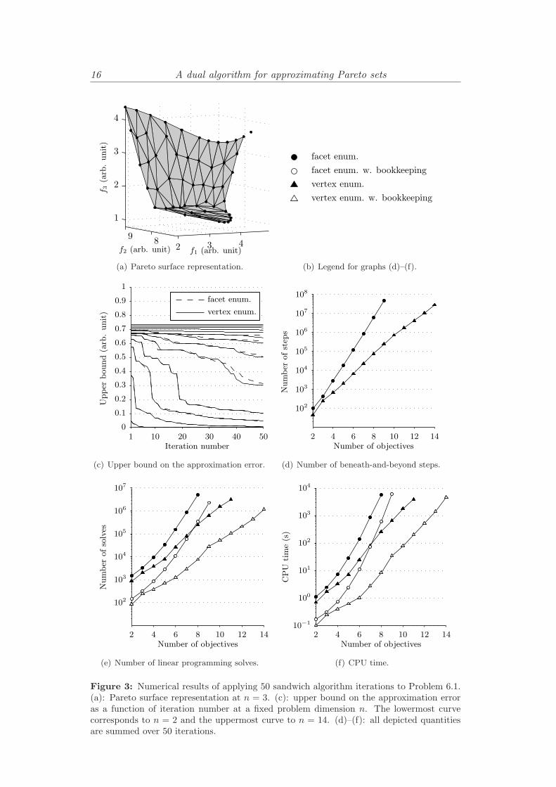
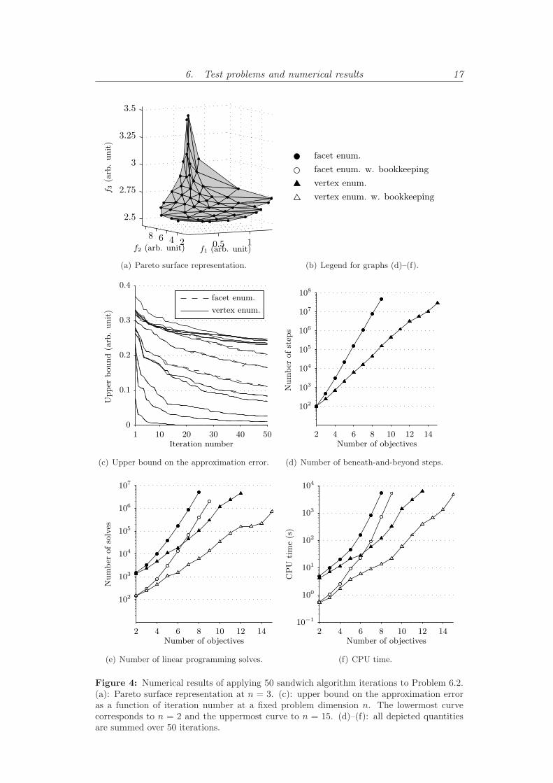
For each problem and algorithm, we report the number of beneath-and-beyondsteps, the number of linear programming solves, and CPU time, summed over 50iterations of the sandwich algorithm. In addition, we report the upper bound onthe approximation error as a function of iteration number. The numerical resultsobtained for Problems 6.1 and 6.2 are summarized in Figure 3 and Figure 4, respec-tively. We stress that our research implementation is not optimized for speed andthe reported running times given only for comparative purposes.

Based on the depicted results, we conclude that the vertex and the facet enu-merative scheme are equivalent in terms of approximation guarantee. In terms ofcomputational load, the combined effect of the vertex enumerative scheme and theproposed upper-bounding procedure results in an improvement that is increasingwith problem dimension. For the two studied problems, the proposed enhance-ments translates into a reduction in the number of linear programming solves byone order of magnitude for dimensions beyond two, and a reduction by two orders ofmagnitude for dimension beyond five. Correspondingly, the number of dimensionstractable at computational times within the order of minutes increases from aboutsix to eleven.


f3(arb.unit)

f2 (arb. unit) f1 (arb. unit)2 3 489

1

2

3

4

(a) Pareto surface representation.

vertex enum. w. bookkeeping

vertex enum.

facet enum. w. bookkeeping

facet enum.

(b) Legend for graphs (d)–(f).

vertex enum.

facet enum.

Upper

bound(arb.unit)

Iteration number1 10 20 30 40 50

0

0.1

0.2

0.3

0.4

0.5

0.6

0.7

0.8

0.9

1

(c) Upper bound on the approximation error.

Number

ofstep

s


102

103

104

105

106

107

108

(d) Number of beneath-and-beyond steps.

Number

ofsolves


102

103

104

105

106

107

(e) Number of linear programming solves.

CPU

time(s)


10−1

100

101

102

103

104

(f) CPU time.

Figure 3: Numerical results of applying 50 sandwich algorithm iterations to Problem 6.1.(a): Pareto surface representation at n = 3. (c): upper bound on the approximation erroras a function of iteration number at a fixed problem dimension n. The lowermost curvecorresponds to n = 2 and the uppermost curve to n = 14. (d)–(f): all depicted quantitiesare summed over 50 iterations.


f3(arb.unit)

f2 (arb. unit) f1 (arb. unit)0.5 12468

2.5

2.75

3

3.25

3.5

(a) Pareto surface representation.

vertex enum. w. bookkeeping

vertex enum.

facet enum. w. bookkeeping

facet enum.

(b) Legend for graphs (d)–(f).

vertex enum.

facet enum.

Upper

bound(arb.unit)

Iteration number1 10 20 30 40 50

0

0.1

0.2

0.3

0.4

(c) Upper bound on the approximation error.

Number

ofstep

s


102

103

104

105

106

107

108

(d) Number of beneath-and-beyond steps.

Number

ofsolves


102

103

104

105

106

107

(e) Number of linear programming solves.

CPU

time(s)


10−1

100

101

102

103

104

(f) CPU time.

Figure 4: Numerical results of applying 50 sandwich algorithm iterations to Problem 6.2.(a): Pareto surface representation at n = 3. (c): upper bound on the approximation erroras a function of iteration number at a fixed problem dimension n. The lowermost curvecorresponds to n = 2 and the uppermost curve to n = 15. (d)–(f): all depicted quantitiesare summed over 50 iterations.


7. Summary and discussion

We have proposed a sandwich algorithm for approximating the Pareto surface of aconvex multi-objective optimization problem based on enumerating the vertices ofan outer polyhedral approximation of the Pareto surface. The proposed method isin a sense dual to a previously suggested algorithm based on enumerating the facetsof the inner approximation. The two enumerative schemes were further enhancedwith an upper-bounding procedure for reducing the number of subproblem solvesrequired to solve a nonconvex optimization problem. This procedure was madepossible by implementing the polyhedral computations in an on-line fashion.

The vertex and the facet enumerative algorithms are both exact methods formaximizing the improvement in bound on the approximation error when generatinga single Pareto optimal solution. As a result, the two methods are equivalent interms of quality of output, as was verified experimentally. The vertex enumerativescheme was shown to improve upon both worst-case complexity and practical per-formance of the sandwich algorithm. This improvement can be attributed to thefact that the vertex enumerative approach handles the normal vectors of the innerapproximation, which is the more structurally complex polyhedron of the inner andouter approximations, as a free variable in the linear programming subproblems. Inthe facet enumerative approach, these normal vectors are instead explicitly given inthe statement of its subproblems, leading to more costly polyhedral computationsand a larger number of subproblems that needs to be solved.

We conclude by summarizing the implications for the IMRT application. Thereis yet no widely accepted consensus on acceptable computational time for generatinga discrete representation of the Pareto surface for this application. However, judgingby a recent clinical evaluation [15] where total planning time was in the order of tenminutes, running times much beyond a number minutes appears unrealistic. Basedon our numerical experience, solving the Pareto surface approximation problem inpresence of the up to about ten problem dimensions that are of interest in IMRTappears tractable in view of the proposed enhancements. We thus envisage thatsandwich algorithms will allow for better resolved models of the viable treatmentoptions in the form of more accurately represented Pareto surfaces throughout thespectrum of problem formulations encountered in IMRT optimization.

A. Formulation of problem 6.2

The patient volume was discretized into 5 × 5 × 5 mm3 volume elements (voxels)and the beam planes into 1× 1 cm2 surface elements (bixels). Dose kernels for fivecoplanar photon beams at equispaced gantry angles were computed using a pencilbeam convolution technique based on singular value decomposition, similar to [4].The problem was posed on the form (2.1) by taking the elements of x to be the energyfluence per bixel and introducing a nonnegativity bound x ≥ 0. All objectives andconstraints were modeled by minimum and a maximum dose functions on the form

g(x) =∑

i∈S

∆viΘ(pTi x, dref)

(

pTi x− dref)2

,

References 19

where S indexes the voxels included in the anatomical structure to which the func-tion is assigned, ∆vi denotes the relative volume of the ith voxel with respect to S,pi is a pencil beam kernel such that di = pTi x, and where Θ(di, d

ref) = (dref−di)+ forminimum dose functions and Θ(di, d

ref) = (di − dref)+ for maximum dose functions.The target structure was assigned with a minimum and a maximum dose ob-

jective with dref = 70 Gy and a minimum dose constraint with dref = 63 Gy. Amaximum dose objective was introduced with dref = 0 Gy for each healthy struc-ture contained in the projection of the target volume onto the beam planes. Theresulting total number of objectives was 15. A constraint on global maximum doseat dref = 77 Gy was introduced by sampling 2 % of all voxels in the patient volumeuniform at random, as to keep running times reasonable. The problem was posedas an inequality constrained quadratic program with 5416 variables and 6937 linearconstraints by introducing auxiliary variables, see [8].

Scaling in the number of objectives was performed by aggregating positivelycorrelated objectives. Each objective was first optimized individually. Objectivesfor healthy structures where then aggregated into composite functions being thedirect sum of all constituent functions by iteratively grouping together the twoobjectives showing maximum degree of mutual monotonocity, as determined bymaximum Spearman rank correlation, see, e.g., [29].

Acknowledgements

The authors thank Bjorn Hardemark and Henrik Rehbinder for valuable discussionduring the course of this work. We also thank Goran Sporre for careful reading andcomments that improved the manuscript.

References

[1] A. Ahnesjo, B. Hardemark, U. Isacsson, and A. Montelius. The IMRT information process—mastering the degrees of freedom in external beam therapy. Physics in Medicine and Biology,51(13):R381–R402, 2006.

[2] R. Bellman. Adaptive Control Processes: A Guided Tour. Princeton University Press, 1961.

[3] T. Bortfeld. IMRT: a review and preview. Physics in Medicine and Biology, 51(13):R363–R379,2006.

[4] T. Bortfeld, W. Schlegel, and B. Rhein. Decomposition of pencil beam kernels for fast dosecalculations in three-dimensional treatment planning. Medical Physics, 20(2):311–318, 1993.

[5] J. Branke, K. Deb, K. Miettinen, and R. Slowinski. Multiobjective Optimization—Interactive

and Evolutionary Approaches. LNCS 5252, State-of-the-Art Survey. Springer, 2008.

[6] D. Bremner, K. Fukuda, and A. Marzetta. Primal-dual methods for vertex and facet enumer-ation. Discrete and Computational Geometry, 20:333–357, 1998.

[7] R. Burkard, H. Hamacher, and G. Rote. Sandwich approximation of univariate convex func-tions with an application to separable convex programming. Naval Research Logistics, 1991.

[8] F. Carlsson, A. Forsgren, H. Rehbinder, and K. Eriksson. Using eigenstructure of the Hessianto reduce the dimension of the intensity modulated radiation therapy optimization problem.Annals of Operations Research, 148(1):81–94, 2006.

[9] C. Cotrutz, M. Lahanas, C. Kappas, and D. Baltas. A multiobjective gradient-based doseoptimization algorithm for external beam conformal radiotherapy. Physics in Medicine and

Biology, 46(8):2161–2175, 2001.

20 References

[10] D. Craft. Calculating and controlling the error of discrete representations of Pareto surfacesin convex multi-criteria optimization. Physica Medica, 26(4):184–191, 2010.

[11] D. Craft and T. Bortfeld. How many plans are needed in an IMRT multi-objective plandatabase? Physics in Medicine and Biology, 53(11):2785–2796, 2008.

[12] D. Craft, T. Halabi, and T. Bortfeld. Exploration of tradeoffs in intensity-modulated radio-therapy. Physics in Medicine and Biology, 50(24):5857–5868, 2005.

[13] D. Craft, T. Halabi, H. Shih, and T. Bortfeld. Approximating convex Pareto surfaces inmultiobjective radiotherapy planning. Medical Physics, 33(9):3399–3407, 2006.

[14] D. Craft, T. Halabi, H. Shih, and T. Bortfeld. An approach for practical multiobjectiveIMRT treatment planning. International Journal of Radiation Oncology, Biology, Physics,69(5):1600–1607, 2007.

[15] D. Craft, T. Hong, H. Shih, and T. Bortfeld. Improved planning time and plan quality throughmulti-criteria optimization for intensity modulated radiation therapy. International Journal

of Radiation Oncology, Biology, Physics, Forthcoming 2011.

[16] D. Craft and M. Monz. Simultaneous navigation of multiple Pareto surfaces, with an applica-tion to multicriteria IMRT planning with multiple beam angle configurations. Medical Physics,37(2):736–741, 2010.

[17] I. Das and E. Dennis. A closer look at drawbacks of minimizing weighted sums of objectives forPareto set generation in multicriteria optimization problems. Structural and Multidisciplinary

Optimization, 14:63–69, 1997.

[18] S. Dempe. Foundation of Bilevel Programming. Nonconvex optimization and its applications.Kluwer Academic, 2002.

[19] H. Edelsbrunner. Algorithms in Combinatorial Geometry. Springer-Verlag, 1987.

[20] M. Ehrgott. Multicriteria Optimization, volume 491 of Lecture Notes in Economics and Math-

ematical Systems. Springer Verlag, 2nd edition, 2005.

[21] A. Engau. Tradeoff-based decomposition and decision-making in multiobjective programming.European Journal of Operational Research, 199(3):883–891, 2009.

[22] P. Eskelinen, K. Miettinen, K. Klamroth, and J. Hakanen. Pareto navigator for interactivenonlinear multiobjective optimization. OR Spectrum, 32:211–227, 2010.

[23] B. Fruhwirth, R. E. Bukkard, and G. Rote. Approximation of convex curves with applicationto the bicriterial minimum cost flow problem. European Journal of Operational Research,42(3):326–338, 1989.

[24] P. E. Gill, W. Murray, and M. A. Saunders. SNOPT: An SQP algorithm for large-scaleconstrained optimization. SIAM Review, 47(1):99–131, 2005.

[25] B. Grunbaum. Convex Polytopes. Springer, 2nd edition, 2003.

[26] T. Hong, D. Craft, F. Carlsson, and T. Bortfeld. Multicriteria optimization in intensity-modulated radiation therapy treatment planning for locally advanced cancer of the pancreatichead. International Journal of Radiation Oncology, Biology, Physics, 72(4):1208–1214, 2008.

[27] B. Hunt and M. Wiecek. Cones to aid decision making in multicriteria programming. InT. Tanino, T. Tanaka, and M. Inuiguchi, editors, Multi-Objective Programming and Goal Pro-

gramming, pages 153–158. Springer Verlag, 2003.

[28] M. Hunt, C. Hsiung, S. Spirou, C. Chui, H. Amols, and C. Ling. Evaluation of concave dosedistributions created using an inverse planning system. International Journal of Radiation

Oncology, Biology, Physics, 54:953–962, Nov 2002.

[29] M. Kendall. Rank Correlation Methods. Griffin, 1962.

[30] K. Klamroth, J. Tind, and M. Wiecek. Unbiased approximation in multicriteria optimization.Mathematical Methods of Operations Research, 56:413–437, 2003.

References 21

[31] K.-H. Kufer, A. Scherrer, M. Monz, F. Alonso, H. Trinkaus, T. Bortfeld, and T. Christian.Intensity-modulated radiotherapy—a large scale multi-criteria programming problem. OR

Spectrum, 25:223–249, 2003.

[32] M. Lahanas, E. Schreibmann, and D. Baltas. Multiobjective inverse planning for intensitymodulated radiotherapy with constraint-free gradient-based optimization algorithms. Physicsin Medicine and Biology, 48(17):2843, 2003.

[33] A. Madansky. Inequalities for stochastic linear programming problems. Mangagement Science,6(2):197–204, 1960.

[34] R. Marler and J. Arora. The weighted sum method for multi-objective optimization: newinsights. Structural and Multidisciplinary Optimization, 41:853–862, 2010.

[35] P. McMullen. The maximum number of faces of a convex polytope. Mathematika, 17(2):179–184, 1970.

[36] K. Miettinen. Nonlinear Multiobjective Optimization. Kluwer Academic, 1999.

[37] M. Monz. Pareto Navigation—Interactive Multiobjective Optimisation and its Application in

Radiotherapy Planning. PhD thesis, University of Kaiserslautern, 2006.

[38] M. Monz, K.-H. Kufer, T. R. Bortfeld, and C. Thieke. Pareto navigation—algorithmic founda-tion of interactive multi-criteria IMRT planning. Physics in Medicine and Biology, 53(4):985–998, 2008.

[39] P. M. Pardalos. Enumerative techniques for solving some nonconvex global optimization prob-lems. OR Spectrum, 10:29–35, 1988.

[40] T. Pennanen and J. Eckstein. Generalized Jacobians of vector-valued convex functions. Tech-nical report, Rutgers University, 1997.

[41] F. P. Preparata and M. Shamos. Computational Geometry—An Introduction. Springer-Verlag,1985.

[42] G. Rennen, E. van Dam, and D. den Hertog. Enhancement of sandwich algorithms for approx-imating higher-dimensional convex Pareto sets. INFORMS Journal on Computing, publishedonline before print, December 2, 2010.

[43] R. Rockafellar. Convex Analysis. Princeton University Press, 1970.

[44] E. Romeijn, J. Dempsey, and J. Li. A unifying framework for multi-criteria fluence mapoptimization models. Physics in Medicine and Biology, 49(10):1991–2013, 2004.

[45] G. Rote. The convergence rate of the sandwich algorithm for approximating convex functions.Computing, 48:337–361, 1992.

[46] S. Ruzika and M. Wiecek. Approximation methods in multiobjective programming. Journal

of Optimization Theory and Applications, 126:473–501, 2005.

[47] J. Serna, M. Monz, K.-H. Kufer, and C. Thieke. Trade-off bounds for the Pareto surfaceapproximation in multi-criteria IMRT planning. Physics in Medicine and Biology, 54(20):6299,2009.

[48] R. Solanki, P. Appino, and J. Cohon. Approximating the noninferior set in multiobjective linearprogramming problems. European Journal of Operational Research, 68(3):356–373, 1993.

[49] T. Spalke, D. Craft, and T. Bortfeld. Analyzing the main trade-offs in multiobjective radiationtherapy treatment planning databases. Physics in Medicine and Biology, 54(12):3741–3754,2009.

[50] J. Stoer and C. Witzgall. Convexity and Optimization in Finite Dimensions I. Springer-Verlag,1970.

[51] C. Thieke, K.-H. Kufer, M. Monz, A. Scherrer, F. Alonso, U. Oelfke, P. Huber, J. Debus, andT. Bortfeld. A new concept for interactive radiotherapy planning with multicriteria optimiza-tion: First clinical evaluation. Radiotherapy and Oncology: Journal of the European Society

for Therapeutic Radiology and Oncology, 85(2):292–298, 2007.

Documents

a dual algorithm for approximating pareto sets in convex multi - KTH