4 JULI 0 1,, E Nationa D~tensI Defence nationals

6

A DOPPLER BIN BLANKING CFARPROCESSOR FOR AIRBORNE RADARS

by

G. Vrckovnik and D. Faubert

DEFENCE RESEARCH ESTABLISHMENT OTTAWAREPORT NO. 1073

April 1991Canadg 91-04308 Ottawa

* Noa DWeneCL*+ Defence natonhle

I t

/

A DOPPLER BIN BLANKING CFAR

PROCESSOR FOR AIRBORNE RADARS

by

G. Vrckovnik and D. FaubertAirborne Radar Section

Radar Division

DEFENCE RESEARCH ESTABLISHMENT OTTAWAREPORT NO. 1073

PCN Apdl 1991021 LA Ottawa

ABSTRACT

In this report a novel scheme for adaptively "blanking-out" the radar resolution cellswhich contain high clutter interference is developed and investigated. For the particular set ofradar parameters that are used, a 60 dB clutter peak appears across all of the range gates, andmany of the Doppler bins. If not dealt with, this huge peak severely degrades the performanceof the CFAR processor, and reduces the sensitivity of the system to targets which reside outsideof the clutter region. Our technique consists of adaptively excluding from the decision process,the range-Doppler cells located within this clutter peak region. As a result, the performance inthe noise dominated interference region is greatly enhanced. Blanking out the clutter peak alsoreduces the variation which occurs in the values of the CFAR threshold multiplier over variousgeometric conditions in which the radar may be operated. It is shown that a single value of theCFAR constant can maintain the false alarm rate for large differences in the operatingenvironment of the radar, if Doppler bin blanking is employed. Consequently, a much simplerCFAR processor can be implemented.

RltSUME

Dans ce rapport, une nouvelle m~thode pour dliminer les cellules de rdsolution radarcontenant un haut niveau d'interfdrence est dvelopp e et dtudi~e. Pour l'ensemble desparamtres du radar utilisds, un pic de fouillis de 60 dB apparat dans toutes les cellules deportdes et dans plusieurs cellules Doppler. Sans traitement appropri6, cet 6norme pic de fouillisdegrade srieusement la performance du processeur CFAR et r~duit la sensibilit6 du syst~me auxcibles A l'extdrieur de la zone de haute interference. De fagon adaptive, notre technique consistek exclure du processus de decision la r6gion d'interf6rence l'int~rieur de laquelle il est de toutefagon fort improbable de d6tecter des cibles. La performance du syst~me dans la r6giondomin6e par le bruit thermique s'en trouve grandement am6lior6e. Aussi, l'61imination du picde fouillis r6duit la variation du multiplicateur CFAR quand la g6ometrie dans laquelle le radaropre change. Avec notre technique, une seule valeur de la constante CFAR suffit memelorsque l'environnement dans lequel le radar op re varie beaucoup. Par cons6quent, unprocesseur CFAR beaucoup plus simple peut Wre implantd.

iii

EXECUTIVE SUMMARY

Constant false alarm rate (CFAR) processors are used to prevent automatic detectionradar systems from becoming overloaded with false targets, in the presence of time-varying orunknown interference environments. They maintain the number of false alarms at a levelconsistent with the design goals. Unfortunately, large clutter returns can cause severedegradation in the performance of these processors. The degradation manifests itself as areduction in the ability to detect targets of a given signalto-noise ratio, while maintaining theoverall system false alarm rate. As well, the constant multiplying factor used in CFARprocessors tends to vary as the range-Doppler resolution cell map changes.

In this report a novel adaptive algorithm to exclude the range-Doppler cells which containclutter is developed. This algorithm, when used in conjunction with a CFAR processor, greatlyenhances the system's sensitivity to targets which reside in the clutter-free region of the range-Doppler map. It is also shown that the CFAR multiplier is relatively invariant to changes in thegeometric conditions of the radar, when the adaptive Doppler bin blanking scheme is used. Thisblanking scheme could lead to a simple CFAR processor which would be effective in anypossible clutter environment.

v

TABLE OF CONTENTS

ABSTRACT .............................................. iii

EXECUTIVE SUMMARY ...................................... v

TABLE OF CONTENTS ...................................... vii

LIST OF FIGURES .......................................... viii

LIST OF TABLES .......................................... ix

1.0 INTRODUCTION ......................................... 1

2.0 CFAR DESCRIPTION ...................................... 2

3.0 AIRBORNE RADAR DATA GENERATION ........................ 3

4.0 SIMULATION RESULTS .................................... 74.1 Cell-Averaging (CA-) CFAR .............................. 74.2 Doppler Bin Blanking Cell-Averaging (DBCA-) CFAR ............... 17

5.0 DETECTION PROBABILITIES ............................... 29

6.0 CONCLUSIONS AND RECOMMENDATIONS FOR FURTHER RESEARCH .. 32

REFERENCES ............................................ 34

vii

LIST OF FIGURES

PAGE

Figure 1. Sidelook, Altitude = 100 m 4Figure 2. Forward Look, Altitude = 100 m 4Figure 3. Sidelook, Altitude = 1 km 5Figure 4. Forward Look, Altitude = 1 km 5Figure 5. Sidelook, Altitude = 10 km 6Figure 6. Forward Look, Altitude = 10 km 6Figure 7. Cell Averaging CFAR Processor 8Figure 8. Threshold CDFs - Sidelook, Altitude = 100 m 11Figure 9. Threshold CDFs - Sidelook, Altitude = 1 km 11Figure 10. Threshold CDFs - Sidelook, Altitude = 10 km 12Figure 11. Threshold CDFs - Forward, Altitude = 100 m 12Figure 12. Threshold CDFs - Forward, Altitude = 1 km 13Figure 13. Threshold CDFs - Forward, Altitude = 10 km 13Figure 14. Threshold Values, RGl, Sidelook, 100 m 14Figure 15. Threshold Values, RG1, Sidelook, 1 km 14Figure 16. Threshold Values, RGl, Sidelook, 10 km 15Figure 17. Threshold Values, RG1, Forward, 100 m 15Figure 18. Threshold Values, RGI, Forward, 1 km 16Figure 19. Threshold Values, RG1, Forward, 10 km 16Figure 20. Threshold CDFs - Sidelook, Altitude 100 m 20Figure 21. Threshold CDFs - Sidelook, Altitude 1 km 20Figure 22. Threshold CDFs - Sidelook, Altitude 10 km 21Figure 23. Threshold CDFs - Forward, Altitude 100 m 2"Figure 24. Threshold CDFs - Forward, Altitude 1 km 22Figure 25. Threshold CDFs - Forward, Altitude 10 km 22Figure 26. RG1 Thresholds - Sidelook, Altitude = 100 m 23Figure 27. RG1 Thresholds - Sidelook, Altitude = 1 km 23Figure 28. RG1 Thresholds - Sidelook, Altitude = 10 km 24Figure 29. RG1 Thresholds - Forward, Altitude = 100 m 24Figure 30. RG1 Thresholds - Forward, Altitude = 1 km 25Figure 31. RG1 Thresholds - Forward, Altitude = 10 km 25Figure 32. Threshold CDFs - 0 x 10 Reference Set 27Figure 33. RGI Thresholds - 0 x 10 Reference Set 27Figure 34. Threshold CDFs - 0 x 40 Reference Set 28Figure 35. RGI Thresholds - 0 x 40 Reference Set 28

ix

LIST OF TABLES

PAGE

Table 1. CA-CFAR (4x4) Threshold Multipliers 9Table 2. CA-CFAR (4x4) CFAR Losses 17Table 3. Doppler Blanking CA-CFAR (4x4) Threshold Multipliers 19Table 4. DBCA-CFAR (4x4) CFAR Losses 26Table 5. Threshold Multipliers for Ox10, 0x40 Windows 26Table 6. Detection Probabilities of CA-CFAR and DBCA-CFAR 30Table 7. Detection Probabilities of CA-CFAR and DBCA-CFAR 31

for Case 0 TargetsTable 8. Detection Probabilities of CA-CFAR and DBCA-CFAR 32

for Case 1 Targets

xi

1.0 INTRODUCTION

In modern radar systems, automatic detection schemes compare some function of theenvelope detector output, in a range-Doppler resolution cell, with a threshold number. A targetis declared to be present if the threshold is exceeded. The threshold value is selected to providea false alarm rate consistent with the operational goals, without overloading the radar systemsignal and data processors. Increasing the detection threshold unnecessarily, results in adesensitization of the radar system to target returns.

The threshold value is a product of the ambient interference power and a proportionalityconstant controlling the false alarm rate. Unfortunately, the interference power in real operatingenvironments is not constant because it consists of thermal noise plus the return echoes frommany point, area or extended targets, known as clutter. When the automatic detection schemeassumes a constant interference power, the false alarm probability is extremely sensitive to smallvariations in that interference power [1]. Since all radar systems operate in time-varying, andunknown interference environments, automatic detection schemes which employ fixed thresholdsare not practical.

The problems of automatic target detection in interference environments which areunknown, or time varying, can be reduced with the use of constant false alarm rate (CFAR)processors. A CFAR processor maintains a constant false alarm probability, while maximizingthe detection probability, by estimating the interference power in the resolution cell under test.If the power in this resolution cell exceeds some fixed multiple of the estimated interferencepower, then a target is declared to be present.

In a previous report [2], three different CFAR techniques (cell-averaging, greatest-of, andsmallest-of [3]) were applied to simulated airborne pulse-Doppler radar data. Interferenceenvironments of thermal noise, and thermal noise plus clutter were considered. The interferencepower distribution in the cell under test was assumed to be known, except for the mean powerjui. The distribution family used was exponential, which corresponds to an interferenceenvironment having a Rayleigh-envelope clutter distribution. The same assumptions about theinterference statistics will be made for the work in this report.

It was found in [2] that the CFAR processors worked very well in the thermal noiseenvironment (CFAR losses < 0.6 dB), but a severe peak in the clutter environment causedserious degradations in their performance. In this report, a modification is suggested whichgreatly improves the processors' performance in clutter. By adaptively "blanking out" the range-Doppler resolution cells which contain clutter, the CFAR processor performance becomesequivalent to the excellent performance achieved in the thermal noise environment. Also, byremoving the cells containing clutter, one threshold proportionality constant can be used in anyradar geometry (look angle, altitude etc.) to yield the desired false alarm probability, as opposedto having to compute a new multiplier each time the geometric conditions change.

- 1

2.0 CFAR DESCRIPTION

The CFAR processor estimates the mean power, A, of the interference in the i ' cellunder test. The squared modulus of the signal in the cell under test is then compared to athreshold, T, where

T= Cai1 ()

and C is a constant controlling the probability of false alarm. C is known by several names:the CFAR constant, the threshold multiplier, or the threshold constant. If the actual power inthe cell under test exceeds the threshold in (1), then a target detection is declared.

The value of C which produces a desired false alarm probability of PFA.,, with exact

mean estimation is,

Co = F..(-PFA) (2)

where F.(x) is the unit mean distribution of the exponential distribution family, given by [4]

F,(x) =l1- e-. (3)

Thus the optimal values of C for the desired false alarm probabilities of PAd, = 10"3, and 106,are C. = 8.39 dB and 11.40 dB, respectively. A technique for determining the thresholdmultiplier C, which yields the desired false alarm rate PFAja for any CFAR processor, wasderived by Weber and Haykin [4]. As this technique was described in detail in [21, only a briefsummary will be given here.

The CFAR algorithm being tested estimates the mean power in each cell, j, of eachrange-Doppler map in the ensemble of snapshots. An estimation error for each cell is computedas the ratio a.,, in which jui is the mean power of the cell calculated over the ensemble ofsnapshots. The natural logarithm of the estimation error is computed for all of the cells in theensemble of snapshots, and a global log-estimation-error histogram, ft )(x), is formed.

The system false alarm probability can be determined using this log-error histogram, theCFAR constant C, and knowledge of the distribution family. This results from the fact that PFAis only dependent upon the ratio of the threshold and the mean power, not upon their actualvalues. PFA, as a function of In C, is found by correlating the global log-error histogram withthe function I - F.(e). The log-error histogram need only be taken once, for C = 1, since thelog-error histogram shifts to the right or left, depending upon the value of C. Determining thevalue of C, which yields the desired probability of false alarm, PF,,,,, is a trial and error processinvolving iterative solutions of the correlation. A search algorithm, based upon the VanWijngaarden-Dekker-Brent method [5], was implemented to determine the value of C whichresulted in a false alarm probability within one one-thousandth of the desired probability of falsealarm.

2

The different CFAR techniques all have different biases and variances, hence comparingonly C values between the techniques is meaningless. By forming histograms of the estimatedpowers in each cell ^9, a cumulative distribution function of the estimated powers can be found,F,(x). Once the value of C has been computed, the cumulative distribution function of thethreshold can be found, using (1), from [6],

FT(x) = Fw() (4)

Comparison of the threshold distribution functions, F,(x), can be used to rate theperformance of different CFAR techniques. If FT(x), for one CFAR method, is strictly to theleft (or above) of the FT(x), from another CFAR method, then the first algorithm is betterbecause it will produce a smaller false alarm probability for any value of the return echo power.The horizontal distance between the threshold distributions is the difference in CFAR lossbetween the methods, for a steady target at a detection probability of PD = FT. The absoluteCFAR loss can be found by comparing F7(x) to the distribution of the thresholds for an idealreceiver, in which T = Coi.

3.0 AIRBORNE RADAR DATA GENERATION

The DREO airborne radar simulator (ABRSIM) [7-11] was used to generate theinterference in the Doppler bin outputs, of each range gate, of an airborne pulse-Doppler radar.The relevant radar parameters in the simulation include a pulse width of 3.33 4s and a pulserepetition frequency of 50 kHz. As a result, a total of five contiguous range gates (whosecentres are spaced 500 m apart), and 128 Doppler frequency bins, make up the range-Dopplermap of any particular snapshot.

The simulator was run in its covariance matrix computation mode with the radar flyingat three different altitudes: 100 m, 1 km, and 10 km; and the antenna pointing in two differentdirections : forward looking, and side looking. The aircraft's velocity was 330 m/s in each case.In the covariance matrix computation mode, the simulator computes the cross-correlation matrixof the range gate samples. In effect, this simulator mode computes an ensemble average of aninfinite number of snapshots. The effects of the antenna backlobes and sidelobes are includedin the result. The antenna backlobes were set to a level of -30 dB with respect to the main lobeof the antenna pattern.

Figures 1 through 6 illustrate the resulting covariance mode range-Doppler interferencepowe. maps, generated by the simulator, for the 6 different altitude-look angle combinationsmentioned above. From these figures two distinct regions can be discerned. In all of the plots,there is a very large peak, extending across all 5 range gates, which is surrounded on both sidesby a relatively flat region. This flat region represents the interference power which is dominatedby thermal noise. The large peak contains both surface clutter and thermal noise. In effect, thesystem's performance is clutter limited in the peak region, while noise limited elsewhere.

3

-4-

Figure 1 • Sidelook, Altitude = 1003 m

iii5.

Fiue2•Frad'okSliue=10r

I-.-

Figure 3 Sidelook, Altitude =1 km

Figure 4: Forward Look, Altitude I 1km

5

Figure 5: Sidelook, Altitude =10 km

Figure 6: Forward Look, Altitude = 10 km

6

The clutter dominated region covers the Doppler velocities of + v,,, where v,, is thevelocity of the aircraft, plus an additional spill-over velocity caused by the window used in thedigital signal processing (Blackman-Harris). One can also see the effect of the altitude returnin range gate 2, at altitudes of 1 km (Figures 3 and 4) and 10 km (Figures 5 and 6). The readeris referred to the references on ABRSIM for further details and information regarding thesimulator's output.

It is assumed that the interference return to any cell in any individual burst is a randomvariable, having an exponential distribution, independent of the returns to other cells. This issimulated by generating a sequence of unit mean, exponentially distributed random variables,and assigning one to each cell in the range-Doppler map. After scaling these random numbersby the cell mean value, one snapshot from the ensemble of possible returns is generated. Themaps produced by the simulator, in the covariance matrix mode, represent the cell mean powersfor the range-Doppler maps. Using this technique, it is possible to generate many snapshots ofrange-Doppler maps, for the various look angle, altitude combinations. This large number ofsnapshots ensures statistical accuracy in the CFAR simulation results which follow.

4.0 SIMULATION RESULTS

In this section, we compare the cell-averaging CFAR processor with a modified,"Doppler-Blanked" version of it. Consequently, a review of the cell-averaging CFAR processorand its simulation results is given below, followed by the results of the "Doppler Blanking" cell-averaging CFAR processor.

4.1 Cell-Averaging (CA-) CFAR

A cell-averaging CFAR processor estimates the interference power, in the cell under test,by using the average value of the surrounding reference cells. That is,

where ji is the estimated power of cell i, X is the power in reference cell j, and N is the sizeof the reference cell set. Because targets are not generally centred in a range gate or a Dopplerbin, the range-Doppler cells which immediately surround the test cell are not included in thereference cell set. A further discussion about the reference cell set may be found in [2]. Ablock diagram of a one-dimensional CA-CFAR processor is given in Figure 7.

An inherent assumption of the CA-CFAR processor is that the interference statistics ofeach reference cell are identical to the statistics of the test cell. Consequently, the performanceof the CA-CFAR processor deteriorates when the interference is nonhomogeneous over thereference cell window. The two most common forms of nonhomogeneity are edge effects anddiscrete scatterers [3].

,. 7

Range Gate Samples

Receiver X..I X X. X,

J F_ TestCell

N

C Comparator

T If X > T, j Target

If X < T, No Target

Figure 7: Cell Averaging CFAR Processor

Edge effects arise when the mean cell powers in the reference window undergo a stepchange along some boundary. This usually occurs when two or more different clutterenvironments (ie. land and sea boundary) lie within the reference window.

Two different cases exist for edge effects [12]:

a) If the test cell lies in a region of weak interference, while some of the reference cellsare immersed in the clutter edge, then the threshold will be unnecessarily raised, therebyreducing the probability of detection. This can be the case, even though the cell under test hasa high signal-to-noise ratio. The clutter regions are expanded by approximately half the lengthof the reference window, causing a masking effect to occur within the clutter area, and slightlyoutside of it. The adaptive blanking scheme which we propose can resolve these problemsbecause the clutter region is excluded from the test cell's reference set.

b) If the cell under test is immersed in the clutter edge, but some of the reference cellsare in the clear region, then the probability of false alarm increases dramatically as the edge stepsize increases. This is a serious problem in the design of search radars [13]. Once again, ouradaptive blanking scheme solves this problem because detections are not attempted in the cellswhich reside in the clutter edge.

8

The presence of a large discrete scatterer, in one or more reference window cells, cancause changes in the clutter distribution itself. This generally occurs when one or moreinterfering targets lie within the reference window. The resulting increase in the threshold leveldegrades the detection of the target in the cell under test. The use of an ordered statisticprocessor, in conjunction with our adaptive blanking scheme, should reduce the effects of a largediscrete scatterer [16].

The CA-CFAR processor was tested on each of the six radar geometry conditions. A4 x 4 (range dimension, Doppler dimension) reference cell set was used, and 350 snapshots weregenerated to ensure statistical accuracy. A desired false alarm probability of 10-1 was selectedafter considering the memory limitations and speed of the computer which ran the simulation [2].Results for different reference windows, and different desired false alarm rates, were reportedin [2], for a side-looking radar at an altitude of 100 m.

Table 1 presents the threshold multipliers (C), that were computed for each of the sixcases. Also listed, is the actual false alarm rate that was obtained for the data which wasgenerated. As expected, this rate is close to the desired rate of 103. It is evident from Table1 that the radar geometry has a significant impact upon the value of the threshold multiplier.This is due to the fact that the magnitude of the clutter peak varies as the radar antenna's altitudeand look angle change. Unfortunately, the large variation (6.04 dB) in the threshold multiplierimplies that in order to maintain a constant false alarm probability, the threshold multiplier mustbe recomputed whenever the radar geometry changes. This may or may not be practical,depending upon the platform which carries the radar. Perhaps a look-up table could be used tostore multiplier values for various radar geometries instead of recomputing these numberswhenever conditions change.

RADAR GEOMETRYI C (dB) ACTUAL PFA

Sidelook, Altitude = 100 m 14.258 1.116 x 10'

Sidelook, Altitude = 1 km 13.730 9.7767 x 104

Sidelook, Altitude = 10 km 10.890 1.1116 x 10-3

Forward, Altitude = 100 m 16.928 9.5535 x 10'Forward, Altitude = 1 km 16.603 9.1964 x 0Forward, Altitude = 10 km 12.807 9.1964 x 10'

TABLE 1 : CA-CFAR (4x4) Threshold Multipliers

9

The threshold distribution functions for each of the six cases, and the correspondingoptimal distribution functions, are plotted in Figures 8 to 13. The actual threshold values forthe first range gate, averaged over the ensemble of snapshots, are illustrated in Figures 14 to 19,for each of the six cases. The CFAR losses of the various cases are listed in Table 2 fordetection probabilities of 0.5 and 0.9. These loss values were obtained by comparing theoptimal and actual threshold distribution functions at FT(x) = 0.5 and 0.9, in Figures 8 to 13.

10

Threshold Distributiop Functions

1.00PC to

0.80

0.60

*+444 Optimal0.40 M..- ACFAR (4x4)

0.20

0.00 .........f-140.00 -120.00 -100.00 -80.00 -6.0 -40.00

X (dB)

Figure 8: Threshold CDFs - Sidelook, Altitude =100 m

1.00 - Threshold Distributiop Functions

0.80

0.60

'4-4-4 Optimal0.40 .-- CA-CFAR (4x4)

0.20

0.00 . . . . . . . . -, r - f-140.00 -120.00 -100.00 -80.00 -60.00 -40.00

X (dB)

Figure 9: Threshold CDFs - Sidelook, Altitude = 1 km

Threshold Distributi~x Functions

1.00 f 0

0.80

0.60

'9-'4 Optimal0.40 -.4. C-CFAR (4x4)

0.20

-130.00 -120.00 -110.00 -100.00 -90.00 -80.00X (dB)

Figure 10: Threshold CDFs - Sidelook, Altitude =10 km

1.00 Threshold Distributioji Functions

0.80

0.60

'44Optimal0.40 C~. A-CFAR (4x4)

0.20

0.00 .............-140.00 -120.00 -100.00 -80.00 -60.00 -40.00

X (dB)

Figure 11: Threshold CDFs - Forward, Altitude = 100 m

12

1.00 Threshold Distributioji Functions

0.00 f 0

0.80

*-4-4 Optimal0.40 T 7 :- CRCF (4x4)

0.20

0.00 .. .. .. .-140.00 -120.00 -100.00 -..8 0'.0 60.0 -4600

X (dB)

Figure 12: Threshold CDFs - Forward, Altitude =1 km

1.00 - Threshold Distributiga Functions

0.80

0.60

*4444 Optimal

0.20

0.00 IN I .. . . . . . . . .. . . . . . .-130.00 -120.00 -110.00 -100.00 -90.00 -80.00

X (dB)

Figure 13: Threshold CDFs - Forward, Altitude = 10 km

13

-40.0 Average Range Gate 1. Pe. = 10-3

-60.0

-Interference

CA-CFAR (4x4)S-80.0 '449'Optimal

S-100.0

-L20.0

-140.0 0 .. ... ... . O... . .. ..i .... ... .Doppler Bin Number

Figure 14 Threshold Values, RG1, Sidelook, 100 m

-60.0- Average Range Gate 1. P&6 = 10-3

-80.0-Interference

CA-CFAR (4x4)444Optimal

S-100.0

-120.0

-140.0-0 40 8 2

Doppler Bin Number

Figure 15 Threshold Values, RGl, Sidelook, 1 km

14

-80.0 Average Range Gate 1, Pe. = 1o-3

-90.0

- Interference-100.0 .~-.CA-CFAR (4x4)

'4--9 Optimal

11-110.0

-120.01

130. 0

-140.0 0. . . . .40 . . . O. . . .Doppler Bin Number

Figure 16: Threshold Values, RG1, Sidelook, 10 km

-40.0- Average Range Gate 1. Pr. = 10-3

-60.0-

-Interference

CA-CFAR (4x4)-80. '4--94Optimal

0 8.0

a. -100.0

-120.0

-140.0 . . . . . . . . . . . . . . . . .0 40 80120Doppler Bin Number

Figure 17 : Threshold Values, RGl, Forward, 100 m

-60.0- Average Range Gate 1, Pt. = 10-

-80.0--Interference

CA-CFAR (4x4)P494Optimal

S-100.0-

-120.0-

-140.0,0 40......80 1 10

Doppler Bin Number

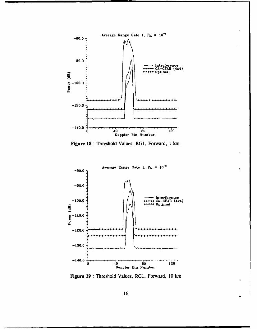
Figure 18 :Threshold Values, RG 1, Forward, 1 km

-80.0 Average Range Gate 1, Pt. = 10-3

-90.0

-Interference

-100.0 .-... CA-CFAR (4x4)P44-* Optimal

~ 110.0

00..

-120.0

-130.0

-140.0 .........I .. .... ... 6Doppler Bin Number

Figure 19 : Threshold Values, RGl, Forward, 10 km

16

CFAR LOSS IN

RADAR GEOMETRY DECIBELS

PD = 0.5 PD-= 0.9

Sidelook, Altitude = 100 m 6.2 16.0

Sidelook, Altitude = 1 km 5.5 11.4

Sidelook, Altitude = 10 km 2.7 4.4

Forward, Altitude = 100 m 8.9 37.0

Forward, Altitude = 1 km 8.4 39.0

Forward, Altitude = 10 km 4.5 27.0

TABLE 2: CA-CFAR (4x4) CFAR Losses

From the threshold plots and Table 2, one can see the effect of the large clutter peak onthe performance of the CFAR processor. As the peak decreases in magnitude (increasingaltitude), the performance of the processor improves. However, even at an altitude of 10 km,the CFAR processor suffers large CFAR losses when the antenna is pointing in the forwarddirection. The mean power of cells, on the peak's edge, is likely to be underestimated by theCFAR processor because the reference cell set, for these edge cells, is made up of low poweredcells, from the noise dominated interference region. Since underestimation of the cell meanpowers contributes most to the CFAR loss [2], it is natural for the performance to degrade inthe presence of a large clutter peak.

As will be illustrated in the next section, another effect of the clutter peak is adesensitization of the radar system in the noise dominated interference region. This occurs asa result of the large threshold multiplier, which is required to maintain the false alarm rate inthe clutter peak region. This large multiplier causes the threshold in the noise region to be muchgreater than it need be, resulting in target desensitization. Virtually all of the false alarms whichoccurred in the simulation (Table 1) took place in the clutter dominated region. Thus, theperformance of the processor clearly would improve, if the clutter peak could be negated. Amethod of achieving this goal is described in the next section.

4.2 Doppler Bin Blanking Cell-Averaging (DBCA-) CFAR

In the previous section, the detrimental effects of the large clutter peak which extendsfrom an approximate Doppler velocity of 500 m/s to -500 m/s, across all five range gates, wereexamined. As a result, it is suggested that detection of targets in the clutter dominated regionnot be attempted. In fact, the bins which contain the clutter should not even be included in the

17

reference cell set for cells in the noise dominated region. In this way, the target detectionproblem is essentially reduced to the detection of a target in the presence of thermal noise.Increased sensitivity in the noise dominated region would be gained, at the expense of a loss oftarget detection capability in the clutter peak. However, due to the large power of the clutterin this peak, it is doubtful as to whether a target could possibly be detected in this clutterbackground in any case. Hence, little system performance would be lost by ignoring the cellswhich reside in the clutter peak.

It is necessary to develop an adaptive method to locate the bounds of the clutter peak,so as to identify the region which needs to be removed, or blanked, from each individual range-Doppler snapshot. Since the clutter peak is present in all of the range gates, a search in theDoppler dimension, along each range line, can be used to determine which Doppler bins needto be removed. By searching along each individual range gate, complete generalization andflexibility can be achieved by the blanking scheme.

The adaptive blanking algorithm, developed for this work, involves two basic steps,which are performed on each range gate of every snapshot: estimating the interference noiselevel, and determining the clutter peak region. The first step is accomplished by averaging theinterference power in the first and last 30 Doppler bins. These 60 bins were selected becausethey are well beyond the region in which the clutter peak may be found (± v,). In order toreduce the effects caused by targets in these Doppler bins, the set of 60 bins may be subdividedinto much smaller subsets of two or three bins for averaging. The resulting means from thesubsets can then be averaged to obtain an estimate of the background noise floor. Should anysubset have a significantly larger mean power than the rest, then it should be excluded from theoverall average because it likely contains a target, not just noise.

Once the interference noise power has been approximated, the width of the clutter peakcan be estimated. A search is performed, from the positive frequency noise-dominated region(eg. Doppler bin 30) to the centre of the Doppler spectrum (bin 64), for the rising edge of theclutter peak, and from the negative frequency noise-dominated region (eg. bin 90) to thespectrum centre, for the falling edge. The beginning (or end) of the peak is considered to bethe first Doppler bin which fulfils a particular "peak location" condition. This condition issatisfied when three consecutive Doppler bins possess interference powers which are greater thanthree decibels above the estimated noise floor. Note that the "peak location" condition may bemade more or less stringent, by varying the required number of consecutive Doppler bins whichmust exceed the noise floor, or by changing the number of decibels, by which the interferencein the Doppler bins must exceed the estimated noise level.

This adaptive Doppler bin blanking algorithm was implemented in conjunction with a 4x4reference window cell-averaging CFAR processor. In Table 3, the threshold multipliers, wflichwere computed for each of the six radar geometry configurations, are listed. Note that the falsealarm rate obtained with the simulated data is close to the desired false alarm rate of 10- .

18

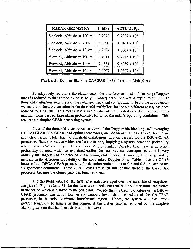
RADAR GEOMETRY C (dB) j ACTUAL PF,

Sidelook, Altitude = 100 m 9.2972 9.2027 x 10'

Sidelook, Altitude 1 km 9.1090 1.0161 x 10.

Sidelook, Altitude = 10 km 9.2631 1.0061 x 10.

Forward, Altitude = 100 m 9.4017 9.7213 x 10'

Forward, Altitude = 1 km 9.1881 9.6039 x 10'

Forward, Altitude = 10 km 9.1097 1.0327 x 10-'

TABLE 3 : Doppler Blanking CA-CFAR (4x4) Threshold Multipliers

By adaptively removing the clutter peak, the interference in all of the range-Dopplermaps is reduced to that caused by noise only. Consequently, one would expect to see similarthreshold multipliers regardless of the radar geometry and configurati, n. From the above table,we see that indeed the variation in the threshold multiplier, for the six different cases, has beenreduced to 0.293 dB. This means that a single value of the threshold constant can be used tomaintain some desired false alarm probability, for all of the radar's operating conditions. Thisresults in a simpler CFAR processing system.

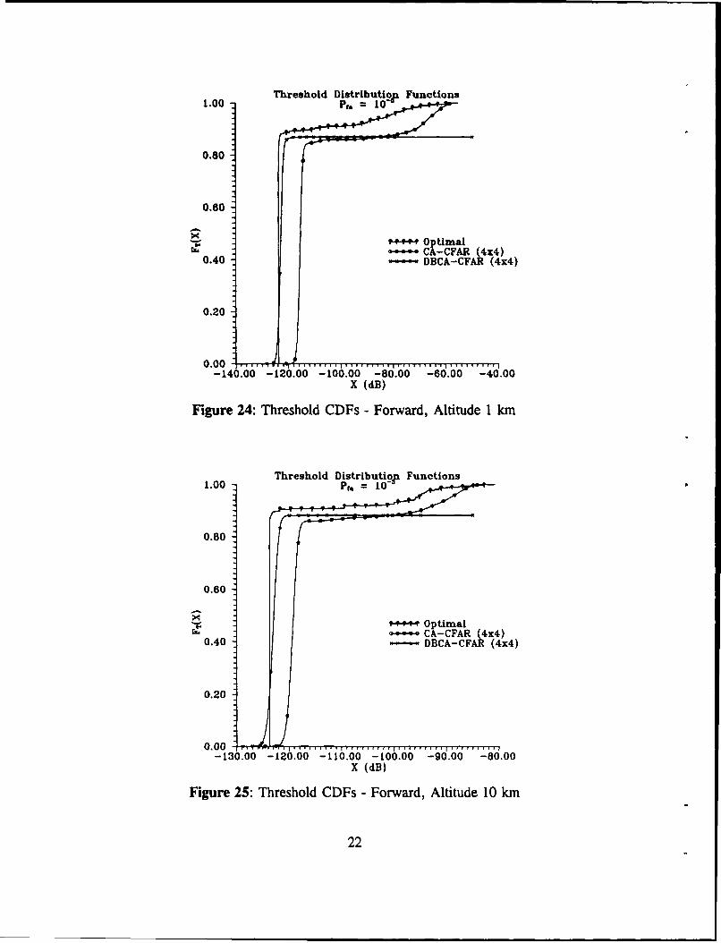
Plots of the threshold distribution function of the Doppler-bin-blanking, cell-averaging(DBCA) CFAR, CA-CFAR, and optimal processors, are shown in Figures 20 to 25, for the sixgeometric cases. Note that the threshold distribution function curves, for the DBCA-CFARprocessor, flatten at values which are less than one, implying a system detection probabilitywhich never reaches unity. This is because the blanked Doppler bins have a detectionprobability of zero, which as explained earlier, has no practical consequence, as it is veryunlikely that targets can be detected in the strong clutter peak. However, there is a rarkedincrease in the detection probability of the nonblanked Doppler bins. Table 4 lists the CFARlosses of this DBCA-CFAR processor, for detection probabilities of 0.5 and 0.8, in each of thesix geometric conditions. These CFAR losses are much smaller than those of the CA-CFARprocessor because the clutter peak has been removed.

The threshold values of the first range gate, averaged over the ensemble of snapshots,are given in Figures 26 to 31, for the six cases studied. No DBCA-CFAR thresholds are plottedin the region which is blanked by the processor. We see that the threshold values of the DBCA-CFAR processor are about four to six decibels lower than the values of the CA-CFARprocessor, in the noise-dominated interference region. Hence, the system will have muchgreater sensitivity to targets in this region, if the clutter peak is removed by the adaptiveblanking scheme that has been derived in this work.

19

1.00 Threshold Distributioju Functions

0.80

0.60

0.40 DBCA-CFA (4x4)

0.20

0.00 .. . . I. . . . . . . . . . I.. . . .-140.00 -120.00 -100.00 -80.00 -60.00 -40.00

X (d0)

Figure 20: Threshold CDFs - Sidelook, Altitude 100 m

Threshold Distributeo Functions1.00 U 1

0.80

0.60

X '4-444Optimal

a.40- CA-CFAR (4x4)0.40 -DBCA-CFAR (4x4)

0.20

0.00-140.00--120.00 -100.00 -80.00 -60.00 -40.00

X (dB)

Figure 21: Threshold CDFs - Sidelook, Altitude 1 km

20

1.00Threshold Distributioji Functions

1.0010

0.80

0.807

*-44 OptimalCA-CFR(4x4)

0.40 ~--DBCA-CFAR (4x4)

0.20

-130.006-100 -110.00 -10 -- 90.00 -80.00X (dB)

Figure 22: Threshold CDFs - Sidelook, Altitude 10 km

1.00 Threshold Distributiop Functions

0.80

0.60

*'44 0O tual

0.40~ - BCA-CFAR (4x4)

0.20

0.00-140.00 -120.00 -1000-8.0 6.0 -40.00

X (dB)

Figure 23: Threshold CDFs - Forward, Altitude 100 m

21

Threshold Distributipo Functions

1.00 f= 07

0.80

0.60

-~ '+V-" 0~ timal

0.40 "--~~DBCA-CFAR (4x4)

0.20

0.00 rr-rrT-rrr .....- 140.00 -120.00 -100.00 -80.00 -60.00 -40.00

X (dB)

Figure 24: Threshold CDFs - Forward, Altitude I km

1.00 Threshold Distributiop Functions

0.80

0.60

94-44 Optimal0- CA-CFAR (4x4)

0.40 -DBCA-CFAR (4x4)

0.20

-130.00 -120.00 -[10.00 -100.00 -90.00 -80.00X (dB)

Figure 25: Threshold CDFs - Forward, Altitude 10 km

22

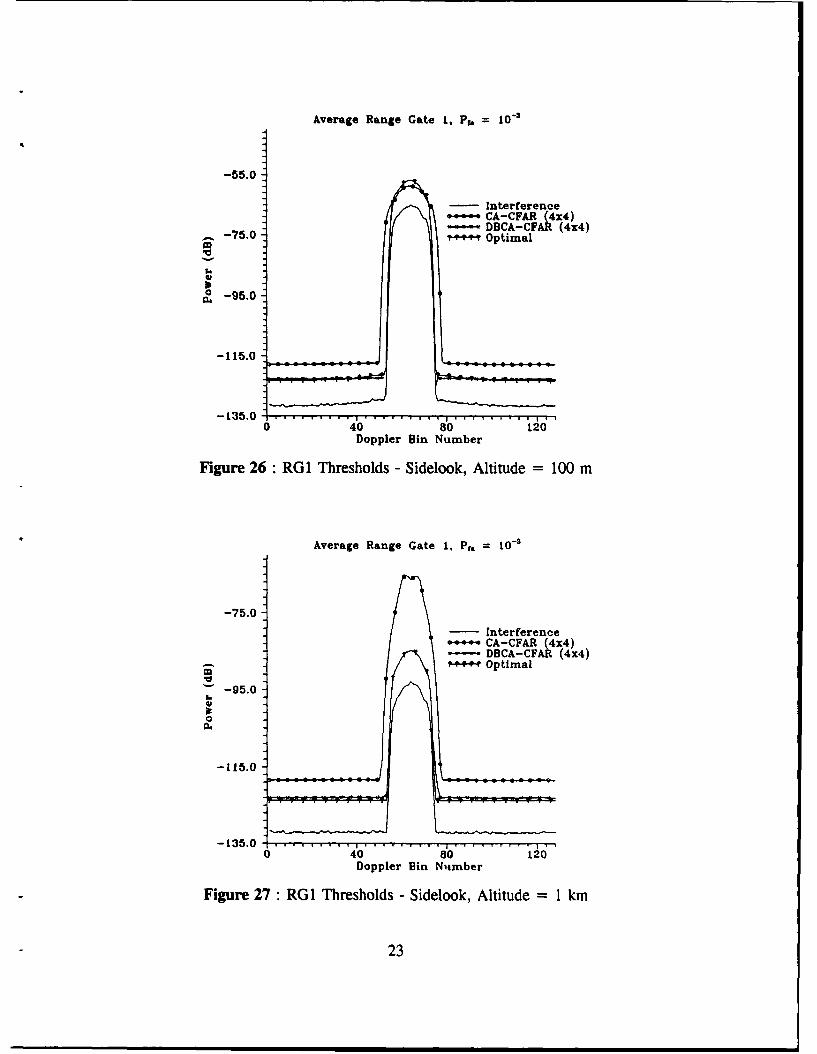
Average Range Gate 1. ,. = 10'

-55.0-

-Interference

CA-CFAR (4x4)-75.0 DBCA-CFAR (4x4)

'-~-~Optimal

S-95.0

-115.0

-135.0a

Doppler Bin Number

Figure 26 RG1 Thresholds - Sidelook, Altitude = 100 m

Average Range Gate 1, P,, = 10-'

-75.0-

-Interference

CA-CFAR (4x4)-DBCA-CFAR (4x4)'-cOptimal

-95.0a.6

0

-135.0 . . . . . . . . . . .0 40 8012

Doppler Bin Nnmber

Figure 27 : RG1 Thresholds - Sidelook, Altitude = 1 km

23

Average Range Gate 1. Pt. = 10-

-85.0

-95.0 - InterferenceCA-CFAR (4x4)DBCA-CFAR (4x4)

'~-'Optimal

-105.0

-115.0

-125.0

0 40 8Doppler Bin Number

Figure 28 :RGL Thresholds - Sidelook, Altitude =10 km

Average Range Gate 1. Pt. = 10-3

-55.0-

-Interference

CA-CFAR (4x4)

-75.0DBCA-CFAR (4x4)-75.0 *-'- Optimal

-135.0.. . . .0 40 so 120

Doppler Bin Number

Figure 29: RG1 Thresholds - Forward, Altitude = 100 m

24

Average Range Gate 1, Pt. = 10-3

-75.0-

-Interference

CA-CFAR (4x4)DBCA-CFAR (4x4)

444Optimal

-95.0

-115.0

-135.0 . . .. . .0 40 8012Doppler Din Number

Figure 30: RGI Thresholds - Forward, Altitude I km

*Average Range Gate 1, P,. = 10-3

-85.0-

-95.0 Interference~-4CA-CFAR (4x4)- DBCA-CFAI (4x4)

- '4444Optimal

'105.0

-115.0

-125.0,

-1500 40 6'0 120Doppler Bin Number

Figure 31 :RG1 Thresholds - Forward, Altitude = 10 km

25

CFAR LOSS IN

RADAR GEOMETRY DECIBELS

PD = 0.5 PD = 0.8

Sidelook, Altitude = 100 m 1.2 1.4

Sidelook, Altitude = 1 km 1.25 1.45

Sidelook, Altitude = 10 km 1.0 2.3

Forward, Altitude = 100 m 1.3 2.0

Forward, Altitude = 1 km 0.9 1.95

Forward, Altitude = 10 km 0.8 1.75

TABLE 4: DBCA-CFAR (4x4) CFAR Losses

In a previous report [2], it was found that good performance could be achieved throughthe use of one-dimensional Doppler reference windows. Consequently, the CA-CFAR andDBCA-CFAR processors were also compared using reference windows, which were one-dimensional in the Doppler dimension. In Table 5, the threshold multipliers, computed for thesidelook case at an altitude of 100 m, are listed for each processor. Reference window sizes ofOxlO and 0x40 cells, and a false alarm rate of 10-1 have been used in calculating the table. Plotsof the threshold distribution functions, and the threshold values for the first range gate, averagedover the ensemble of snapshots, are given in Figures 32 to 35. Once again, from these figuresit is evident that the DBCA-CFAR processor outperforms the CA-CFAR processor. Also, asthe number of cells in the reference window increases (from 10 to 40), the performance of theDBCA-CFAR processor improves. This is intuitively satisfying, as one would expect anestimate of the mean noise level to improve as the number of samples, used in forming theestimate, increases.

CFAR REFERENCE SET C (dB) ACTUAL PA

CA-CFAR 0 x 10 10.300 1.0536 x 10.'

CA-CFAR 0 x 40 13.802 1.0268 x 10.3

DBCA-CFAR 0 x 10 10.315 1.0084 x 10'

DBCA-CFAR 0 x 40 8.980 9.0374 x 10-4

TABLE 5 : Threshold Multipliers for Ox10, 0x40 Windows

26

P,=1-

1.0 0 x 10 Window

0.9

0.7

0.6 -- 444" OptimalCA-CFAR

0.5 ~DBCA-CFARC-.

0.4

0.3

0.2

0.1

-140 -120 -100 -80 -60 -0X (dB)

Figure 32 Threshold CDFs - 0 x 10 Reference Set

pta = 10-Range Gate I

- S. 00-

-Interference Power9-44Optimal Threshold-CA OxtO Threshold

*-75.00 .- e DBCA OxlO Threshold

U

S-95.00

-115.00

-3S. 000.00 40.0 80.00... 120.00

Doppler Bin Number

Figure 33 RGl Thresholds - 0 x 10 Reference Set

27

P =1 3

1.0 0 x 40 Window

0.9

0.8

0.7

0.6 "- ia

S0.5 DBCA-CFAR

0.4-

0.3

0.2

0.1

-140 -0 -10 -0 60 -40

X (dB)

Figure 34: Threshold CDFs - 0 x 40 Reference Set

Pt. = 1-

Range Gate 1

Interference PowerS Optimal Threshold

k C1 Ox4O Threshold~ -75.00DBCA 0x40 Threshold

9500

11 -5.00

-D.

0.00 40.00 80. 00 100Doppler Bin Number

Figure 35 :RG 1 Thresholds - 0 x 40 Reference Set

28

5.0 DETECTION PROBABILITIES

In this section, the detection probabilities of targets of various strengths are obtainedthrough simulation, and compared to theoretical predictions. Non-fluctuating, Swerling Case 0targets [14] are considered first, followed by Swerling Case 1 fluctuating targets.

To perform detection probability estimates, the CFAR simulator was modified to allowthe addition of a steady target to any of the individual range-Doppler cells. A signal, which iscomposed of a non-fluctuating target plus thermal noise, has a Rician power distribution, asopposed to the exponential power distribution of thermal noise alone [15]. Consequently, anadjustment was made to the simulator to obtain the proper power distribution function, in thecell in which the target resides.

Targets, with various signal-to-noise ratios, were placed in a particular range-Dopplercell, and their detection probabilities were determined by comparing the target cell's power tothe threshold computed for that cell. If the cell's power exceeded the threshold, then a detectionwas declared, otherwise a missed detection was declared. This process was repeated for 10000snapshots, at which point an estimate of the target's detection probability was obtained. Notethat 10000 snapshots yielded estimates which were consistent within approximately onepercentage point.

The increased sensitivity to targets, of DBCA-CFAR over CA-CFAR, in the noise-dominated interference region, was demonstrated by calculating the detection probabilities oftargets with signal-to-noise ratios of 0,2,4,6,8,10, and 12 dB. The target was placed in Dopplerbin 35 of the first range gate for all of the cases. The results are listed in Table 6, along withthe theoretical optimal detection probabilities, obtained from Meyer and Mayer [14]. We cansee that in general, as expected, the DBCA-CFAR processor yields much larger detectionprobabilities than the CA-CFAR processor. This is because of the smaller CFAR loss, whichis incurred by the DBCA-CFAR processor, and which results in smaller threshold values for anygiven false alarm rate.

One can confirm the operation of the CFAR simulator, by increasing the target's signalto noise ratio (SNR) by the corresponding processor's CFAR loss. If this is done, then thedetection probability should be essentially equivalent to the theoretical value, obtained with anoptimal processor, for a target with the original SNR. From the plots of the actual thresholdvalues in the first range gate, it is possible to estimate the additional SNR required to obtainoptimal operation, for a target placed in Doppler bin 35. The extra SNR, required for the CA-CFAR processor with reference windows of 4x4, and OxlO cells, is approximately 5.5 dB, and2.0 dB, respectively. Note that a 0x40 window, for the CA-CFAR processor, is not consideredin this test because of the very large CFAR loss (about 48 dB), associated with this referencewindow. For the DBCA-CFAR processor, the additional SNRs are 0.5 dB, 2.0 dB, and 0.75dB, for reference windows of 4x4, OxlO, and 0x40 cells, respectively. Consequently, thedetection probability of a CA-CFAR processor using a 4x4 reference window, for a target SNRof 5.5 dB, should be equivalent to an optimal processor detecting a target whose SNR is 0.0 dB.

29

In Table 7, detection probabilities of an optimal processor, for target SNRs of 0,2,4,6,8,10, and12 dB, are compared with the CA and DBCA-CFAR processors, whose target SNRs have beenincreased by the additional SNR mentioned above. From this table, it is clear that by increasingthe target's SNR, by an amount equal to the CFAR loss of the processor, the detection rate thatwould have been obtained using an optimal processor can be achieved. Hence the simulator isworking properly.

PERCENTAGE PROBABILITY OF DETECTION

TARGET CA-CFAR I DBCA-CFAR

.SNR (dB) O1PTMAL 4- 0 0 0x4 x x 0 Ox40]4x4 0 xl0 0x40 J4x4 J0xl0 0x40_

0.0 1.8 0.02 0.75 0.00 2.91 0.75 1.36

2.0 4.0 0.03 1.58 0.00 5.46 1.54 2.79

4.0 9.75 0.07 3.60 0.00 11.74 3.60 6.91

6.0 23.5 0.18 9.18 0.00 24.82 9.18 16.98

8.0 49.0 0.92 23.60 0.00 49.69 23.50 39.11

10.0 81.0 5.34 50.76 0.00 80.02 50.68 71.90

12.0 97.8 24.67 81.61 0.00 96.83 81.60 95.00

TABLE 6: Detection Probabilities of CA-CFAR and DBCA-CFAR

Finally, some results using Swerling Case 1 targets are presented. Swerling Case 1targets possess a Rayleigh distributed amplitude, which fluctuates on a scan to scan basis [14].In Table 8, the detection probabilities, obtained for the CA-CFAR processor, with referencewindows of 4x4 and OxlO cells, and the DBCA-CFAR processor, with reference windows of4x4, Ox10, and 0x40 cells, are given. Note that the target signal to noise ratios have beenincreased by the processors' CFAR loss, as with the Case 0 targets, to facilitate a comparisonwith an optimal processor. Targets with SNRs of 0,2,4,6,8,10, and 12 dB were used. Onceagain, there is agreement between the theoretical detection probabilities, and the detectionprobabilities obtained with the CFAR processors, after the CFAR loss has been included in thetarget's signal to noise ratio.

The small discrepancies between the theoretical detection probabilities, and the simulationresults, are believed to be caused by several factors. First, recall that the 10000 snapshots, usedto determine the detection rates, produce results which are only consistent to within onepercentage point. Inaccurate estimation of the CFAR loss contributes to the error, since even

30

slight variations of the threshold may cause significant variation in the detection probability.This effect is enhanced for targets with small signal-to-noise ratios. Finally, we note that thedetection probabilities obtained are 'local' probabilities. That is, detection was only consideredfor a target in one particular range-Doppler resolution cell, out of the entire map of cells. Amore accurate, 'global', detection probability estimate could be obtained by placing the targetin each resolution cell of the map, in turn. This is similar to the manner in which the thresholdmultiplier was computed. Recall that the estimation errors of every cell, in every snapshot,contribute to the determination of the threshold constant. Analogously, a 'global' detectionprobability could be obtained. However, this exercise would be extremely time consuming, andsomewhat redundant, as a global detection rate can already be computed by using the thresholddistribution functions [4]. Hence, little would be gained by conducting a massive simulation tocompute 'global' detection probabilities.

PERCENTAGE PROBABILITY OF DETECTIONOPTIMALTARGET CA-CFAR DBCA-CFAR

SNR (dB) OPTIMAL IT4x4 Oxt1 4x4 iOx I 0x40

0.0 1.8 0.06 1.59 2.95 1.60 1.62

2.0 4.0 0.51 3.82 6.28 3.88 3.63

4.0 9.75 3.18 9.55 13.87 9.50 8.76

6.0 23.5 17.08 23.53 29.34 23.50 23.12

8.0 49.0 55.51 50.15 56.44 50.27 50.99

10.0 81.0 93.57 81.80 85.45 81.81 82.79

12.0 97.8 99.96 97.76 98.56 97.74 98.18

TABLE 7: Detection Probabilities of CA-CFAR and DBCA-CFAR for Case 0 Targets

31

PERCENTAGE PROBABILITY OF DETECTIONOPTIMALTARGET CA-CFAR DBCA-CFAR

SNR (dB) OPTIMAL 4x4 O 4x4 Ox 10 x40

0.0 3.1 0.87 0.88 0.85 0.86 0.44

2.0 7.0 4.23 4.04 4.21 4.03 3.31

4.0 14.0 10.72 10.65 10.59 10.67 9.21

6.0 25.0 23.77 21.98 23.48 22.03 20.16

8.0 39.0 37.85 36.03 37.58 36.15 34.96

10.0 54.0 53.58 51.61 53.30 51.64 51.24

12.0 66.5 67.40 65.29 67.17 65.37 65.11

TABLE 8 Detection Probabilities of CA-CFAR and DBCA-CFAR for Case 1 Targets

6.0 CONCLUSIONS AND RECOMMENDATIONS FOR FURTHER RESEARCH

This report has been an extension of some previous work which was conducted by theauthors at DREO [2]. For the particular radar parameters considered, a very large clutter peak(60 dB) extends across all of the range gates, and a segment of the Doppler bins. The returnsin the Doppler bins are confined to velocities between the velocity of the radar platform itself,and its corresponding negative value. This clutter peak severely hampers the effectiveness ofa CFAR processor, by reducing the sensitivity of the system to targets residing outside of theclutter region. The likelihood of being able to detect any target in this huge clutter return isvery small indeed.

Consequently, it was suggested that the range-Doppler cells which contain the clutter beignored, or 'blanked-out'. In this way, the processor's operating environment is simplified tothat required for thermal noise only. A fully adaptive scheme was developed to determine whichrange-Doppler cells contained the clutter peak, and subsequently, which ones could be ignoredin any further processing. By combining this blanking scheme with standard cell-averagingCFAR, substantial reductions in the processor's CFAR loss were achieved. It was shown thatthe processor which employed the blanking algorithm was much more sensitive to targets in thenoise-dominated region of the range-Doppler map.

With the blanking scheme, a single value of the CFAR constant can be used to maintainsome desired false alarm rate, in virtually any geometric operating condition of the radar. The

32

cases which were studied, explicitly included two cases of an airborne radar: one with side-looking, and one with forward-looking antennas. They also included consideration of these twocases at three different altitudes: 100m, 1 kin, and 10 km. While the standard CA-CFARprocessor's threshold multiplier, exhibited a large variation over these various conditions, theDoppler bin blanking CA-CFAR processor had very little variation. Consequently, there maybe no need to recompute the multiplier whenever the geometric parameters change, if theDoppler bin blaaking algorithm is used.

Finally, the detection probabilities of non-fluctuating and Swerling Case 1 fluctuatingtargets were computed, and found to agree with theoretical predictions. This confirmed theproper operation of the CFAR simulator which has been developed.

Future research could investigate the advantages of combining the Doppler bin blankingalgorithm, with greatest-of, or ordered statistic CFAR processors [3,16]. In this way, target selfmasking problems [2,4,12,16] could be reduced, while still benefitting from the performanceimprovement, obtained through the removal of the clutter peak. Additionally, the Doppler binblanking algorithm, which has been developed in this report, could be applied to a different setof radar parameters, in which the clutter peak may not be as broad, or strong. This wouldfacilitate testing of the performance of the blanking algorithm, in conjunction with a CFARprocessor, in the presence of discrete scatterers, or targets of strength comparable to the clutterreturns.

33

REFERENCES

1. Finn H.M., and Johnson R.S., Adaptive Detection Mode with Threshold Control as aFunction of Spatially Sampled Clutter-Level Estimates, RCA Review, Vol. 29, No. 3,September 1968, pp. 414-464.

2. Vrckovnik G., and Faubert D., An Investigation of CFAR Techniques for AirborneRadars, DREO Report No. 1056, Defence Research Establishment Ottawa, Ottawa,December 1990.

3. Minkler G., and Minider J., CFAR : The Principles of Automatic Radar Detection inClutter, Magellan Book Company, Baltimore, MD, 1990.

4. Weber P., Haykin S., and Gray R., Airborne Pulse-Doppler Radar. False-AlarmControl, lEE Proceedings, Vol. 134, Pt. F, No. 2, April 1987, pp. 127-134.

5. Press W.H., Flannery B.P., Teukolsky S.A., and Vetterling W.T., Numerical Recipes- The Art of Scientific Computing, Cambridge University Press, Cambridge, 1986.

6. Meyer P.L., Introductory Probability and Statistical Applications (Second Edition),Addison-Wesley Publishing Company, Reading MA, 1970.

7. Faubert D., A Theoretical Model for Airborne Radars, Defence Research EstablishmentOttawa Report No. 1017, PCN 21LA12, November 1989.

8. Vineberg K.A., and Saper R., Updates to the DREO Airborne Radar Simulator,Atlantis Scientific Systems Group Inc. Report No. 167, June 1989.

9. Gibb M., Lightstone L., and Saper R., Pulse Doppler Radar Simulation Study: FinalTechnical Report, Atlantis Scientific Systems Group Inc. Report No. TR-20, October1988.

10. Lightstone L., Behaviour of the SIR for Space-Based DPCA Radar Under VariousSpatial Clutter Distributions, Atlantis Scientific Systems Group Inc. Report No. TR- 11,February 1988.

11. Lightstone L., A Model of a Displaced Phase Centre Antenna System for Space-BasedRadar with Generalized Orbital Parameters and Earth Rotation, Atlantis ScientificSystems Group Inc., Contract Number W7714-06-5121, July 1987.

12. Weiss M., Analysis of Some Modified Cell-Averaging CFAR Processors in Multiple-Target Situations, IEEE Transactions on Aerospace and Electronic Systems,Vol. AES-18, No. 2, March 1982, pp. 242-248.

34

13. Hansen V.G., Constant False Alarm Rate Processing in Search Radars, IEE ConferencePublication No. 105, "Radar-Present and Future", London, October 23-25 1973,pp. 325-332.

14. Meyer D.P., and Mayer H.A., Radar Target Detection - Handbook of Theory andPractice, Academic Press, New York, 1973.

15. Haykin S., Communication Systems, Second Edition, John Wiley and Sons, New York,1983.

16. Rohling H., Radar CFAR Thresholding in Clutter and Multiple Target Situations, IEEETransactions on Aerospace and Electronic Systems, Vol. AES-19, No. 4, July 1983,pp. 608-621.

35

NC, IFIET) F D

SECURITY CLASSIFICATION OF FORM(higts classification of Title, Abstract, Keywords)

DOCUMENT CONTROL DATA(Security classification of title, body of -bstrsct ind indexing annotation must be entered when the overall document is classified)

1. ORIGINATOR (the no and adress of the rgoization preparing the document 2. SECURITY CLASSIFICATIONOrganizations for whom the document wa prepared, e.g. Establishment sponsoring (overall security classification of the documenta contrac s report, or tasking agency, re entered in section 8.) including special warning terms if applicable)

Defence Research Establishment Ottawa3701 Carling Avenue UNCLASSIFIED

Ottawa, Ontario, Canada KIA OZ4

3. TITLE (the complete document title as indicated on the title page. Its classification should be indicated by the appropriateabbreviation (SC or U) in parentheses after the title.)

A Doppler Bin Blanking CFAR Processor for Airborne Radars (U)

4. AUTHORS ast name. first name, middle initial)

VRCKOVNIK Gary E., FAUBERT Denis

5. DATE OF PU3LICATION (month and year of publication of 6& NO. OF PAGES (total 6b. NO. OF REFS (total cited indocument) containing information. Include document)

March 1991 Annexes, Appendices, etc.) 1642

7. DESCRIPTIVE NOTES (the category of the document, e.g. technical report, technical note or memorandum. If appropriate, enter the type ofreport, e.g. interim, progress. summary, annual or final. Give the inclusive dates when a specific reporting period is covered.)

DREO Technical Report

8. SPONSORING ACTIVITY (the name of the department project office or laboratory sponsoring the research and development Include theaddress.) Defence Research Establishment Ottawa

3701 Carling AvenueOttawa, Ontario, Canada KIA 0Z4

9a PROJECT OR GRANT NO. (if appropriate, the applicable research 9b. CONTRACT NO. (if appropriate, the applicable number underand development project or grant number under which the document which the document was written)was writterL Please specify whether project or grant)

021LA

10a. ORIGINATORS DOCUMENT NUMBER (the official document 10b. OTHER DOCUMENT NOS. (Any other numbers which maynumber by which the document is identified by the originating be assigned this document either by the originator or by theactivity. This number must be unique to this document) sponsor)

DREO Report 1073

11. DOCUMENT AVAILABILITY (any limitations on further dissemination of the document, other than those imposed by security classification)

(X) Unlimited distribution

Distribution limited to defence departments and defence contractors; further distribution only as approvedDistribution limited to defence departments and Canadian defence contractors; further distribution only as approved

( Distribution limited to government departments and agencies; further distribution only as approvedDistribution limited to defence departments; further distribution only as approved

I ) Other please specify):

12. DOCUMENT ANNOUNCEMENT (any limitation to the bibliographic announcement of this document This will normally correspond tothe Document Availabilty (11). However, where further distribution (beyond the audience specified in 11) is possible, a widerannouncement audience may be selected)

UNCLASSIFIED

SECURITY CLASSIFICATION OF FORM

DCD03 2106187

-38- UNCLASSIFIEDSECURITY CLASSIFICATION OF FORM

13. ABSTRACT ( a brief md factual summwy of the document It may also appear elsewhere in the body of the document itself. It is highlydesirable tha the abstract of classified docwnments be unclassified. Each paragraph of the abstract shall begin with an indication of thesecurity classification of the information in the paragraph (unless the document itself is unclassified) represented as (S). (C), or (U).It is not necessary to include here abstracts in both officl languages unless the txt is bilingual).

In this report a novel scheme for adaptively "blanking-out" the radarresolution cells which contain high clutter interference is developed andinvestigated. For the particular set of radar parameters that are used, a 60 dB

clutter peak appears across all of the range gates, and many of the Doppler bins.

If not dealt with, this huge peak severely degrades the performance of the CFAR

processor, and reduces the sensitivity of the system to targets which reside

outside of the clutter region. Our technique consists of adaptively excluding fromthe decision process the range-Doppler cells located within this clutter peakregion. As a result, the performance in the noise dominated interference region isgreatly enhanced. Blanking out the clutter peak also reduces the variation whichoccurs in the values of the CFAR threshold multiplier over various geometric

conditions in which the radar may be operated. It is shown that a single value ofthe CFAR constant can maintain the false alarm rate for large differences in theoperating environment of the radar, if Doppler bin blanking is employed.Consequently, a much simpler CFAR processor can be implemented.

14. KEYWORDS. DESCRIPTORS or IDENTIFIERS (technically meaningful terms or short phrases that characterize a document and could behelpful is caalagWi4the docurmne They should be selected so that no security classification is required. Identifiers. such as equipmentmodel designaton, trade name, militpry pirqjet. code name, geographic location may also be included. If possible keywords should be selectedfrom a published thes*s._ e.g. Thesurs of.- Engingring and Scientific Terms (TEST) and that thesaurus-identified. If it is not possible toselect indexing .-t~s °fll~'"are Unlassified, the €lssif Iation of each should be indicated as with the title.)

Constant false alarm rate processors, CFAR, Cell-averaging,

Airborne pulse-Doppler radar, clutter cancellation

UNCLASSIFIED

SIECURITY CLASSIFICATION OF FORM