A distributed model of blowing snow over complex terrain

A distributed model of blowing snow overcomplex terrain

Richard Essery,1 Long Li1 and John Pomeroy2*1Division of Hydrology, University of Saskatchewan, Saskatoon, Saskatchewan, Canada, S7N 0W0

2National Hydrology Research Centre, Saskatoon, Saskatchewan, Canada S7N 3H5

Abstract:Physically-based models of blowing snow and wind¯ow are used to develop a distributed model of blowingsnow transport and sublimation over complex terrain. The model is applied to an arctic tundra basin. A

reasonable agreement with results from snow surveys is obtained, provided sublimation processes are included;a simulation without sublimation produces much greater snow accumulations than were measured. The modelis able to reproduce some observed features of redistributed snowcovers: distributions of snow mass, classi®ed

by vegetation type and landform, can be approximated by lognormal distributions, and standard deviations ofsnow mass along transects follow a power law with transect length up to a cut-o�. The representation used forthe downwind development of blowing snow with changes in windspeed and surface characteristics is found to

have a large moderating in¯uence on snow redistribution. Copyright # 1999 John Wiley & Sons, Ltd.

KEY WORDS blowing snow; snow transport; sublimation; snow distribution; snow surveys; complex terrain

INTRODUCTION

Large amounts of wind-blown snow can sublimate in open environments, and redistribution of snow bywind can lead to large variations in depth which in¯uence the depletion of snow during melt (Donald et al.,1995; Shook, 1995). Transport and sublimation rates increase rapidly with increasing windspeed and so arehighly sensitive to windspeed variations caused by variations in topography and roughness. In this paper,results from the Prairie Blowing SnowModel (Pomeroy, 1988; Pomeroy et al., 1993; Pomeroy and Li, 1999a)and the MS3DJH/3R terrain wind¯ow model (Walmsley et al., 1982, 1986; Taylor et al., 1983) are used todevelop a distributed model of blowing snow over complex terrain. The model is applied to Trail ValleyCreek, an arctic tundra basin 50 km north of Inuvik, NWT, using half-hourly meteorological data. Suchfrequent measurements, although valuable for modelling non-linear blowing snow processes, are rarelyavailable for arctic locations; previous distributed blowing snow models have been driven with monthly(Pomeroy et al., 1997) or daily (Liston and Sturm, 1998) data.

The Prairie Blowing Snow Model (PBSM) is a physically-based model that calculates transport andsublimation rates for blowing snow over uniform terrain given measurements of air temperature, humidityand windspeed. Data requirements and the complexity of its algorithms make PBSM unsuitable for use indistributed models, so a simpli®ed blowing snow model (`SBSM'), which can reproduce PBSM results veryclosely with much less computational e�ort, is used. The requirement for distributed meteorological data isaddressed, in part, by using MS3DJH/3R to produce wind¯ow maps; other atmospheric variables areassumed to be homogeneous over the model domain. Lacking a physically-based model of blowing snow

CCC 0885±6087/99/142423±16$17�50 Received 7 October 1998Copyright # 1999 John Wiley & Sons, Ltd. Revised 4 January 1999

Accepted 11 March 1999

HYDROLOGICAL PROCESSESHydrol. Process. 13, 2423±2438 (1999)

*Correspondence to: John Pomeroy, National Hydrology Research Centre, Saskatoon, Saskatchewan, Canada, S7N 3H5.

development in response to small-scale spatial variations in windspeed and surface characteristics, we haveadopted an ad hoc representation, consistent with available measurements (Takeuchi, 1980), and investigatedthe sensitivity of simulations to its inclusion; the development of blowing snow ¯uxes over homogeneousfetches is a problem of current theoretical interest (DeÂ ry et al., 1998).

Observed snow depths or masses for a redistributed snowcover can often be approximated by a lognormaldistribution (Donald et al., 1995; Shook, 1995; Pomeroy et al., 1998), characterized by a mean and acoe�cient of variation (standard deviation divided by mean). Vegetation and topography in¯uence theredistribution of snow (Pomeroy and Gray, 1995), so di�erent vegetation types and landforms can beexpected to have snow distributions with di�erent parameters, and strati®ed sampling techniques arerequired to obtain accurate estimates of area-average snowmasses for complex terrains (Steppuhn and Dyck,1974). Table I, reproduced from Pomeroy et al. (1998), gives coe�cients of variation (Cv) in snow masscollated from late-winter snow surveys for arctic landscapes with various vegetation types and landforms. Cv

tends to be small for tall, dense vegetation and sheltered locations with little redistribution of snow, andgreater for landforms which cause wind¯ow divergence and consequent erosion and deposition of snow.

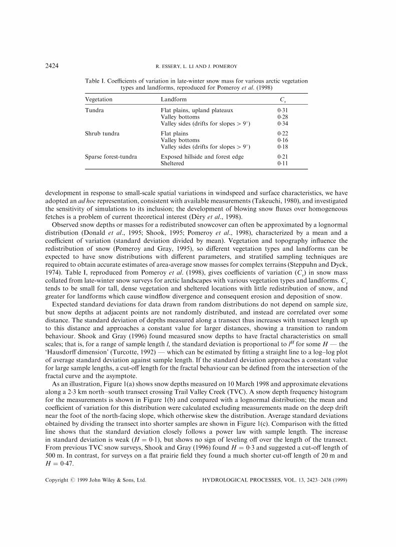
Expected standard deviations for data drawn from random distributions do not depend on sample size,but snow depths at adjacent points are not randomly distributed, and instead are correlated over somedistance. The standard deviation of depths measured along a transect thus increases with transect length upto this distance and approaches a constant value for larger distances, showing a transition to randombehaviour. Shook and Gray (1996) found measured snow depths to have fractal characteristics on smallscales; that is, for a range of sample length l, the standard deviation is proportional to lH for some H Ð the`Hausdor� dimension' (Turcotte, 1992) Ð which can be estimated by ®tting a straight line to a log±log plotof average standard deviation against sample length. If the standard deviation approaches a constant valuefor large sample lengths, a cut-o� length for the fractal behaviour can be de®ned from the intersection of thefractal curve and the asymptote.

As an illustration, Figure 1(a) shows snow depths measured on 10March 1998 and approximate elevationsalong a 2.3 km north±south transect crossing Trail Valley Creek (TVC). A snow depth frequency histogramfor the measurements is shown in Figure 1(b) and compared with a lognormal distribution; the mean andcoe�cient of variation for this distribution were calculated excluding measurements made on the deep driftnear the foot of the north-facing slope, which otherwise skew the distribution. Average standard deviationsobtained by dividing the transect into shorter samples are shown in Figure 1(c). Comparison with the ®ttedline shows that the standard deviation closely follows a power law with sample length. The increasein standard deviation is weak (H � 0.1), but shows no sign of leveling o� over the length of the transect.From previous TVC snow surveys, Shook and Gray (1996) found H � 0.3 and suggested a cut-o� length of500 m. In contrast, for surveys on a ¯at prairie ®eld they found a much shorter cut-o� length of 20 m andH � 0.47.

Table I. Coe�cients of variation in late-winter snow mass for various arctic vegetationtypes and landforms, reproduced for Pomeroy et al. (1998)

Vegetation Landform Cv

Tundra Flat plains, upland plateaux 0.31Valley bottoms 0.28Valley sides (drifts for slopes4 98� 0.34

Shrub tundra Flat plains 0.22Valley bottoms 0.16Valley sides (drifts for slopes4 98� 0.18

Sparse forest-tundra Exposed hillside and forest edge 0.21Sheltered 0.11

Copyright # 1999 John Wiley & Sons, Ltd. HYDROLOGICAL PROCESSES, VOL. 13, 2423±2438 (1999)

2424 R. ESSERY, L. LI AND J. POMEROY

SIMPLIFIED BLOWING SNOW MODEL

The rate of mass transport by blowing snow across a unit width perpendicular to the wind is given by

QT � Qsalt �Z Zb

h*

Z�z�u�z�dz �1�

where Qsalt is the rate of transport by saltation in a layer of depth h, near the surface, u(z) is the windspeed atheight z and Z(z) is the mass concentration of suspended snow, which increases with windspeed but decreaseswith height. The upper boundary for suspended snow, zb , increases with windspeed, surface roughness anddownwind distance.

Despite the complexity of the terms in equation (1), it turns out that PBSM gives transport rates that scaleapproximately as the fourth power of windspeed, with a weak dependence on air temperature through thethreshold windspeed at which blowing snow commences; PBSM uses a quadratic function of temperaturederived from observations of blowing snow occurrence to calculate this threshold (Li and Pomeroy, 1997a).

Figure 1. Results from measurements of snow depth on a north±south transect crossing TVC. (a) Snow depth (lower line) and elevationalong the transect. (b) Frequency histogram for the depths shown in (a), compared with a lognormal distribution. (c) Average standard

deviation of snow depth for samples of length l. The ®tted line is proportional to l 0.1.


SNOW HYDROLOGY 48: MODEL OF BLOWING SNOWFLUXES 2425

In place of the numerical integration used by PBSM to evaluate equation 1, SBSM thus uses an approx-imation of the form

QT � a�T�u410; �2�

where u10 (m sÿ1) is the windspeed at a height of 10 m, T ( 8C) is the air temperature, and the temperaturefunction

a�T� � �1710 � 1�36T� � 10ÿ9 �3�

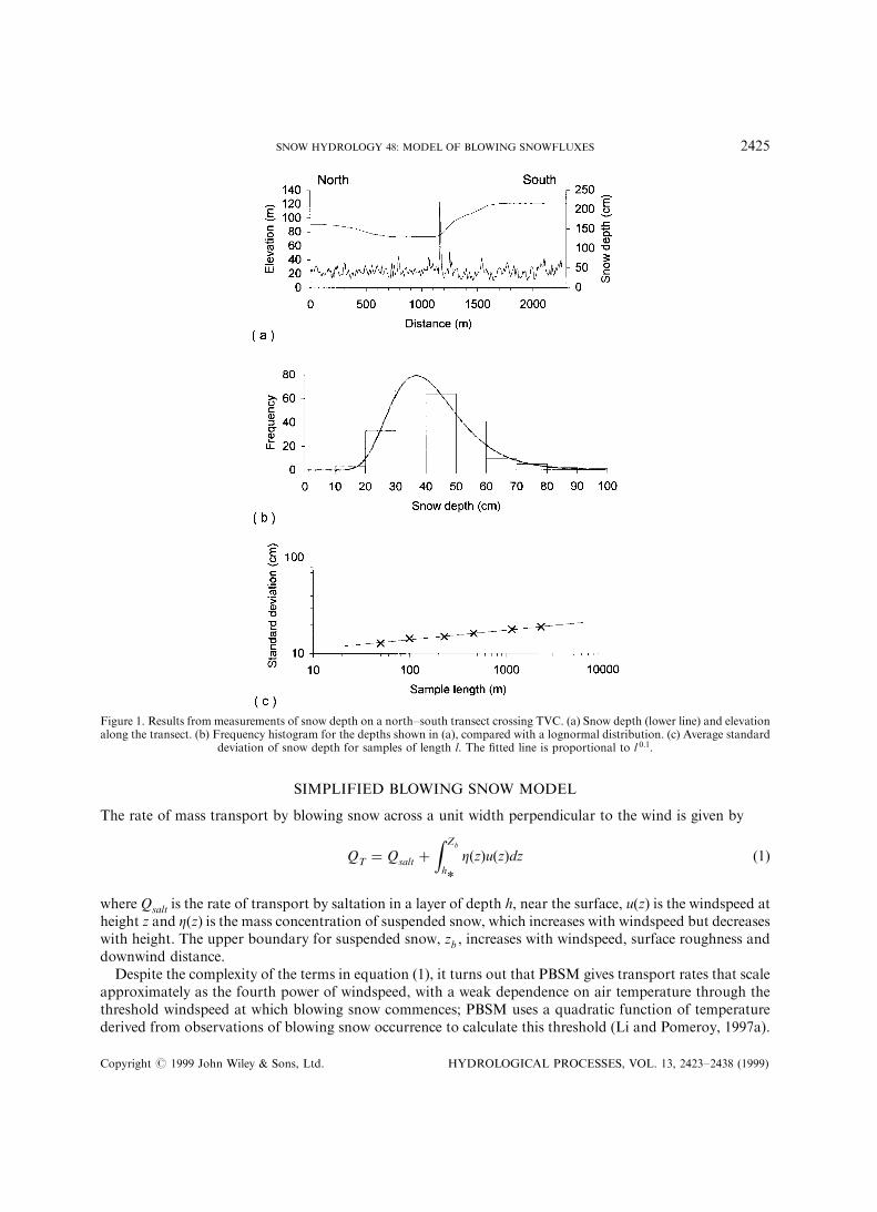
is ®tted to PBSM results. Figure 2 shows how PBSM transport rates, divided by a(T), depend on windspeedover a 1000 m fetch of complete snowcover without exposed vegetation; the ®tted line shows that equation 2gives a good approximation.

PBSM calculates the rate of sublimation from blowing snow over a unit area of ground as

QS �Z zb

0

1

�m�z�d �m

dtZ�z�dz; �4�

where �m(z) is the average blowing snow particle mass at height z, calculated assuming that particle sizesfollow a gamma distribution (Schmidt, 1982). For air temperature T and undersaturation s, Thorpe andMason (1966) give an expression for the rate of mass decrease for a snow particle of mass m and radius r thatcan be written in the form

dm

dt� 2pr Nu

sF�t� ; �5�

where Nu is the Nusselt number and

F�T� � Ls

lT�T � 273�LsM

R�T � 273� ÿ 1

� �� 1

Drs: �6�

F(T) only depends on temperature; Ls is the latent heat of sublimation,M is the molecular weight of water, Ris the universal gas constant, lT is the thermal conductivity of air, D is the di�usivity of water vapour in airand rs is the water vapour saturation density. PBSM includes a second term in equation 5 to allow forshortwave radiation absorbed by snow particles (Schmidt, 1991) but this typically only adds a small

Figure 2. Scaled transport (X) and sublimation (e) rates from PBSM for temperatures between ÿ40 8C and 0 8C and relative humiditiesof 70 percent and 90 percent. The ®tted curves are u4 and u5



correction; neglecting this term, and using the PBSM assumption that the undersaturation at any height isproportional to s2 , the undersaturation at 2 m, equation 4 can be written as

Qs �s2F�T�Q

ls; �7�

where Qls is a scaled sublimation rate. Figure 2 shows that, for a 1000 m fetch, PBSM gives scaled

sublimation rates proportional to u510 but with little dependence on temperature or humidity. SBSM thusreplaces the numerical integration of equation 4 with an approximation

Qs �b s2F�T� u

510; �8�

where b is a constant.To scale from a point to a uniform area, PBSM weights blowing snow ¯uxes by the probability of blowing

snow occurrence (Pomeroy and Li, 1999a). Li and Pomeroy (1997b) found this probability to follow acumulative normal distribution

P�u10� �1��2pp

d

Z u10

0

exp ÿ � �u ÿ u�22d2

� �du; �9�

where, for dry snow of age A (in hours), the parameters of the distribution are given by

�u � 11�2 � 0�365T � 0�00706T2 � 0�9 1n�A� �10�and

d � 4�3 � 0�145T � 0�00196T2: �11�For wet or icy snow, the parameters are taken to be �u � 21 m sÿ1 and d � 7 m sÿ1.

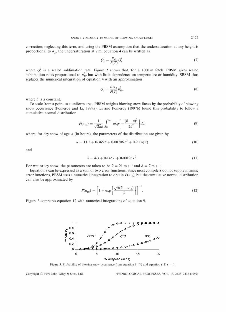
Equation 9 can be expressed as a sum of two error functions. Since most compilers do not supply intrinsicerror functions, PBSM uses a numerical integration to obtain P(u10), but the cumulative normal distributioncan also be approximated by

P�u10� � 1 � exp

��pp � �u ÿ u10�

d

� �� ÿ1: �12�

Figure 3 compares equation 12 with numerical integrations of equation 9.

Figure 3. Probability of blowing snow occurrence from equation 8 (e) and equation (11) ( Ð )



If vegetation extends above the snow, the surface wind stress is partitioned between the snow surface andthe protruding vegetation. Using a stress-partitioning relationship due to Raupach et al. (1993), u10 inequation 12 is replaced by

us �u10

�1 � 340zov�1=2�13�

in this case, where zov is the exposed vegetation roughness length. Lettau (1969) gives

zov �Ndh

2�14�

for vegetation of height h, stalk diameter d and stalk density N. Snow depths are subtracted from h to giveexposed vegetation heights.

TERRAIN WINDFLOW MODEL

Wind¯ow over complex terrain is modelled here using the MS3DJH/3R model developed by Walmsley andco-workers (Walmsley et al., 1982, 1986; Taylor et al., 1983) from theoretical work by Jackson and Hunt(1975) and Mason and Sykes (1979). Linearized momentum equations are solved using Fourier transformsof topography speci®ed by a Digital Elevation Model (DEM). As a linear model, MS3DJH/3R is only validfor ¯ow over low hills with slopes less than about 1 in 4 and assumes neutral strati®cation (studies of blowingsnow generally assume that shear production of turbulence gives neutral strati®cation, but the suppression ofturbulence by suspended snow has been considered by Bintanja, 1998).

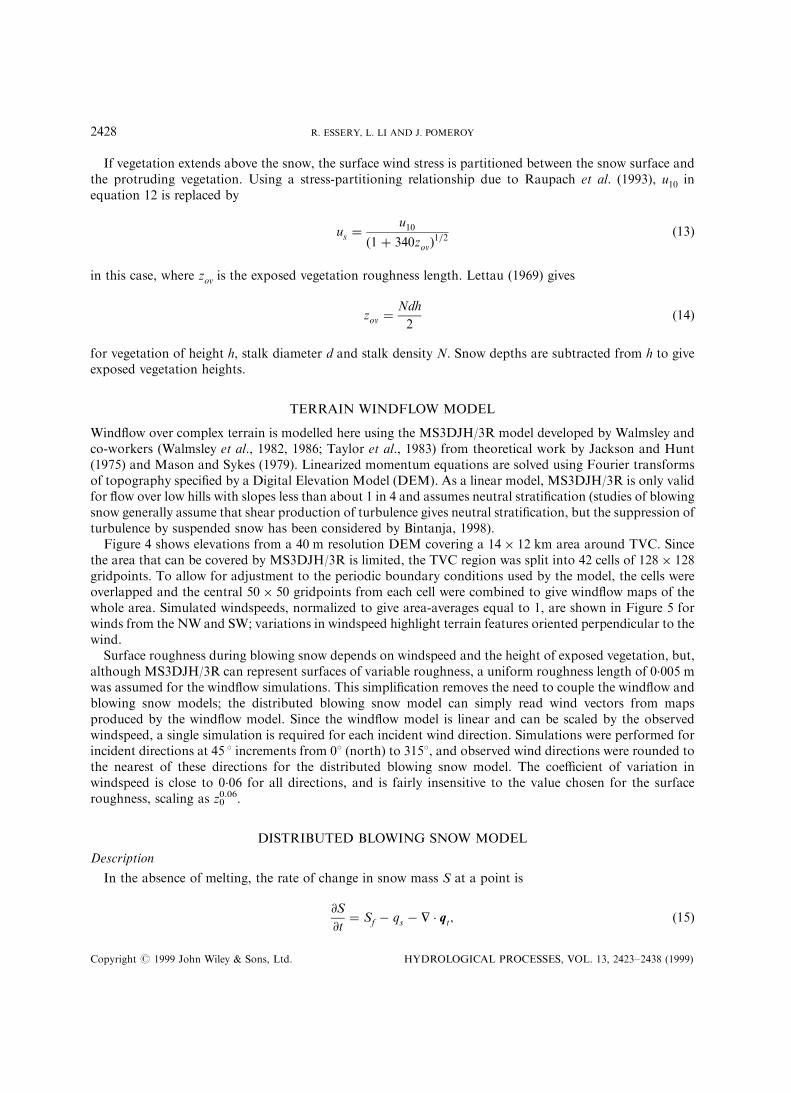
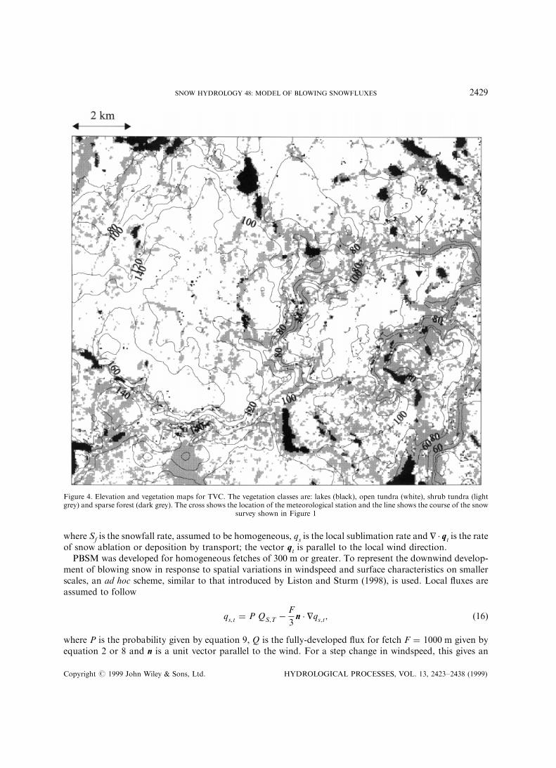
Figure 4 shows elevations from a 40 m resolution DEM covering a 14� 12 km area around TVC. Sincethe area that can be covered by MS3DJH/3R is limited, the TVC region was split into 42 cells of 128� 128gridpoints. To allow for adjustment to the periodic boundary conditions used by the model, the cells wereoverlapped and the central 50� 50 gridpoints from each cell were combined to give wind¯ow maps of thewhole area. Simulated windspeeds, normalized to give area-averages equal to 1, are shown in Figure 5 forwinds from the NWand SW; variations in windspeed highlight terrain features oriented perpendicular to thewind.

Surface roughness during blowing snow depends on windspeed and the height of exposed vegetation, but,although MS3DJH/3R can represent surfaces of variable roughness, a uniform roughness length of 0.005 mwas assumed for the wind¯ow simulations. This simpli®cation removes the need to couple the wind¯ow andblowing snow models; the distributed blowing snow model can simply read wind vectors from mapsproduced by the wind¯ow model. Since the wind¯ow model is linear and can be scaled by the observedwindspeed, a single simulation is required for each incident wind direction. Simulations were performed forincident directions at 45 8 increments from 08 (north) to 3158, and observed wind directions were rounded tothe nearest of these directions for the distributed blowing snow model. The coe�cient of variation inwindspeed is close to 0.06 for all directions, and is fairly insensitive to the value chosen for the surfaceroughness, scaling as z0.060 .

DISTRIBUTED BLOWING SNOW MODEL

Description

In the absence of melting, the rate of change in snow mass S at a point is

@S

@t� Sf ÿ qs ÿ H � qt; �15�



where Sf is the snowfall rate, assumed to be homogeneous, qs is the local sublimation rate and H . qt is the rateof snow ablation or deposition by transport; the vector qt is parallel to the local wind direction.

PBSM was developed for homogeneous fetches of 300 m or greater. To represent the downwind develop-ment of blowing snow in response to spatial variations in windspeed and surface characteristics on smallerscales, an ad hoc scheme, similar to that introduced by Liston and Sturm (1998), is used. Local ¯uxes areassumed to follow

qs;t � P QS;T ÿF

3n � Hqs;t; �16�

where P is the probability given by equation 9, Q is the fully-developed ¯ux for fetch F � 1000 m given byequation 2 or 8 and n is a unit vector parallel to the wind. For a step change in windspeed, this gives an

Figure 4. Elevation and vegetation maps for TVC. The vegetation classes are: lakes (black), open tundra (white), shrub tundra (lightgrey) and sparse forest (dark grey). The cross shows the location of the meteorological station and the line shows the course of the snow

survey shown in Figure 1



Figure 5. Normalized speeds for (a) NW and (b) SW winds



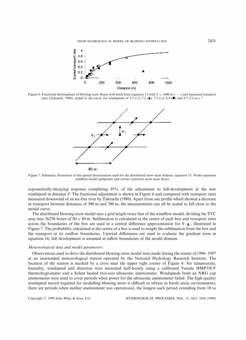
exponentially-decaying response completing 95% of the adjustment to full-development at the newwindspeed in distance F. The fractional adjustment is shown in Figure 6 and compared with transport ratesmeasured downwind of an ice-free river by Takeuchi (1980). Apart from one pro®le which showed a decreasein transport between distances of 300 m and 700 m, the measurements can all be scaled to fall close to themodel curve.

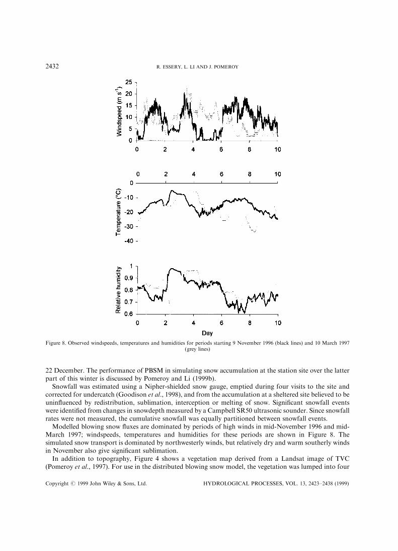
The distributed blowing snowmodel uses a grid length twice that of the wind¯owmodel, dividing the TVCarea into 26250 boxes of 80� 80 m. Sublimation is calculated at the centre of each box and transport ratesacross the boundaries of the box are used in a central di�erence approximation for H . qt , illustrated inFigure 7. The probability calculated at the centre of a box is used to weight the sublimation from the box andthe transport at its out¯ow boundaries. Upwind di�erences are used to evaluate the gradient term inequation 16; full development is assumed at in¯ow boundaries of the model domain.

Meteorological data and model parameters

Observations used to drive the distributed blowing snow model were made during the winter of 1996±1997at an unattended meteorological station operated by the National Hydrology Research Institute. Thelocation of the station is marked by a cross near the upper right corner of Figure 4. Air temperature,humidity, windspeed and direction were measured half-hourly using a calibrated Vaisala HMP35CFthermohygrometer and a Solent heated two-axis ultrasonic anemometer. Windspeeds from an NRG cupanemometer were used to cover periods when power for the ultrasonic anemometer failed. The high-qualitywindspeed record required for modelling blowing snow is di�cult to obtain in harsh arctic environments;there are periods when neither anemometer was operational, the longest such period extending from 10 to

Figure 6. Fractional development of blowing snow ¯uxes with fetch from equation 15 with F � 1000 m ( Ð ) and measured transportrates (Takeuchi, 1980), scaled to the curve, for windspeeds of 5.2 (s), 7.2 (m), 7.3 (n), 8.4 (d) and 8.7 (h) m sÿ1

Figure 7. Schematic illustration of the spatial discretization used for the distributed snow mass balance, equation 15. Nodes representwind¯ow-model gridpoints and arrows represent snow mass ¯uxes



22 December. The performance of PBSM in simulating snow accumulation at the station site over the latterpart of this winter is discussed by Pomeroy and Li (1999b).

Snowfall was estimated using a Nipher-shielded snow gauge, emptied during four visits to the site andcorrected for undercatch (Goodison et al., 1998), and from the accumulation at a sheltered site believed to beunin¯uenced by redistribution, sublimation, interception or melting of snow. Signi®cant snowfall eventswere identi®ed from changes in snowdepth measured by a Campbell SR50 ultrasonic sounder. Since snowfallrates were not measured, the cumulative snowfall was equally partitioned between snowfall events.

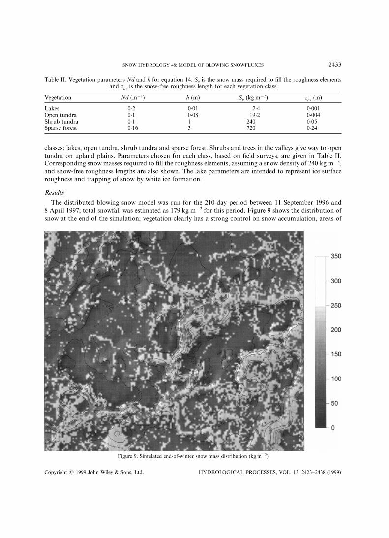
Modelled blowing snow ¯uxes are dominated by periods of high winds in mid-November 1996 and mid-March 1997; windspeeds, temperatures and humidities for these periods are shown in Figure 8. Thesimulated snow transport is dominated by northwesterly winds, but relatively dry and warm southerly windsin November also give signi®cant sublimation.

In addition to topography, Figure 4 shows a vegetation map derived from a Landsat image of TVC(Pomeroy et al., 1997). For use in the distributed blowing snow model, the vegetation was lumped into four

Figure 8. Observed windspeeds, temperatures and humidities for periods starting 9 November 1996 (black lines) and 10 March 1997(grey lines)



classes: lakes, open tundra, shrub tundra and sparse forest. Shrubs and trees in the valleys give way to opentundra on upland plains. Parameters chosen for each class, based on ®eld surveys, are given in Table II.Corresponding snow masses required to ®ll the roughness elements, assuming a snow density of 240 kg mÿ3,and snow-free roughness lengths are also shown. The lake parameters are intended to represent ice surfaceroughness and trapping of snow by white ice formation.

Results

The distributed blowing snow model was run for the 210-day period between 11 September 1996 and8 April 1997; total snowfall was estimated as 179 kg mÿ2 for this period. Figure 9 shows the distribution ofsnow at the end of the simulation; vegetation clearly has a strong control on snow accumulation, areas of

Table II. Vegetation parameters Nd and h for equation 14. Sv is the snow mass required to ®ll the roughness elementsand zov is the snow-free roughness length for each vegetation class

Vegetation Nd (mÿ1) h (m) Sv (kg mÿ2) zov (m)

Lakes 0.2 0.01 2.4 0.001Open tundra 0.1 0.08 19.2 0.004Shrub tundra 0.1 1 240 0.05Sparse forest 0.16 3 720 0.24

Figure 9. Simulated end-of-winter snow mass distribution (kg mÿ2)



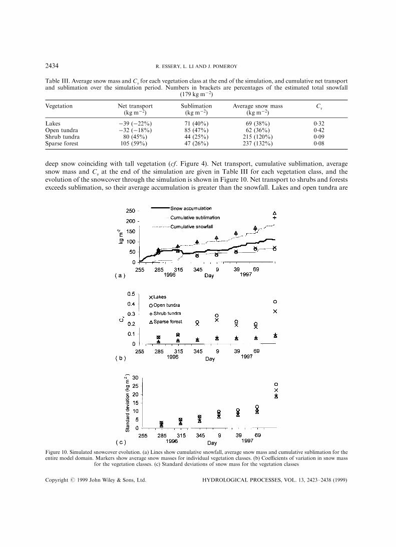
deep snow coinciding with tall vegetation (cf. Figure 4). Net transport, cumulative sublimation, averagesnow mass and Cv at the end of the simulation are given in Table III for each vegetation class, and theevolution of the snowcover through the simulation is shown in Figure 10. Net transport to shrubs and forestsexceeds sublimation, so their average accumulation is greater than the snowfall. Lakes and open tundra are

Table III. Average snow mass and Cv for each vegetation class at the end of the simulation, and cumulative net transportand sublimation over the simulation period. Numbers in brackets are percentages of the estimated total snowfall

(179 kg mÿ2)

Vegetation Net transport Sublimation Average snow mass Cv(kg mÿ2) (kg mÿ2) (kg mÿ2)

Lakes ÿ39 (ÿ22%) 71 (40%) 69 (38%) 0.32Open tundra ÿ32 (ÿ18%) 85 (47%) 62 (36%) 0.42Shrub tundra 80 (45%) 44 (25%) 215 (120%) 0.09Sparse forest 105 (59%) 47 (26%) 237 (132%) 0.08

Figure 10. Simulated snowcover evolution. (a) Lines show cumulative snowfall, average snow mass and cumulative sublimation for theentire model domain. Markers show average snow masses for individual vegetation classes. (b) Coe�cients of variation in snow mass

for the vegetation classes. (c) Standard deviations of snow mass for the vegetation classes



sources of blowing snow; 47% of the snowfall on open tundra sublimates and a further 18% is lost totransport. Lakes are generally located in relatively sheltered low-lying areas and are fringed with shrubswhich trap snow blowing from upwind areas, so lakes on average su�er less sublimation than open tundrabut lose more snow through transport.

Simulated values of Cv are not strictly comparable with survey results (BloÈ schl, 1999), typically calculatedfrom point measurements with spacings of a few metres, but they show the same decrease with increasingvegetation height. Late-winter Cv is observed to be fairly consistent from year to year for a given landscape,but Figure 10(b) shows that coe�cients of variation are rather variable through the course of the simulation.Standard deviations, shown in Figure 10(c), increase monotonically with time and are similar for allvegetation classes. Although Cv determines the shape of the snowcover depletion curve during melt for anassumed lognormal distribution of pre-melt snow mass (Donald et al., 1995; Shook, 1995), the standarddeviation may be the more appropriate parameter for describing the development of a snowcover duringredistribution by wind.

Snow surveys were carried out in open tundra, shrub tundra and forest areas on 23 April 1997; averagesnow masses and standard deviations are given in Table IV. The simulated snow mass for open tundraappears to be underestimated, but all model averages lie within one standard deviation of the survey results.A simulation with transport but no sublimation gives much greater snow accumulations than weremeasured Ð 141 kg mÿ2 for open tundra, 270 kg mÿ2 for shrub tundra and 608 kg mÿ2 for forests Ðsuggesting that sublimation is a signi®cant component of the snow mass budget for TVC.

Topographic drifts surveyed at TVC, such as that shown in Figure 1, are generally too narrow to beresolved by the distributed model grid, but some topographic in¯uence is evident in Figure 11, which showsaverage snow masses on open tundra as a function of aspect for slopes of greater and less than 9 8. Theaccumulation is greatest on slopes in the lee of the dominant NW winds and least on windward slopes. Areasof shrub tundra are able to trap more snow than open tundra and show no strong relationship between snowaccumulation and slope or aspect in the simulation.

The distribution of snow within each vegetation class is shown by snow mass frequency histograms inFigure 12. These distributions are not lognormal, but can be better approximated by sums of lognormals if

Table IV. Results from snow surveys on 23 April 1997

Vegetation Average snow mass Standard deviation Cv(kg mÿ2) (kg mÿ2)

Open tundra 86 27 0.31Shrub tundra 219 42 0.19Forest 215 49 0.23

Figure 11. Average snow mass as a function of slope and aspect for open tundra from the simulation shown in Figure 9



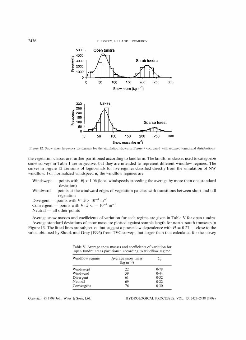
the vegetation classes are further partitioned according to landform. The landform classes used to categorizesnow surveys in Table I are subjective, but they are intended to represent di�erent wind¯ow regimes. Thecurves in Figure 12 are sums of lognormals for ®ve regimes classi®ed directly from the simulation of NWwind¯ow. For normalized windspeed uÃ, the wind¯ow regimes are:

Windswept Ð points with juj4 1�06 (local windspeeds exceeding the average by more than one standarddeviation)

Windward Ð points at the windward edges of vegetation patches with transitions between short and tallvegetation

Divergent Ð points with H � u4 10ÿ4 mÿ1

Convergent Ð points with H � u5 ÿ 10ÿ4 mÿ1

Neutral Ð all other points

Average snow masses and coe�cients of variation for each regime are given in Table V for open tundra.Average standard deviations of snow mass are plotted against sample length for north±south transects in

Figure 13. The ®tted lines are subjective, but suggest a power-law dependence with H � 0.27 Ð close to thevalue obtained by Shook and Gray (1996) from TVC surveys, but larger than that calculated for the survey

Figure 12. Snow mass frequency histograms for the simulation shown in Figure 9 compared with summed lognormal distributions

Table V. Average snow masses and coe�cients of variation foropen tundra areas partitioned according to wind¯ow regime

Wind¯ow regime Average snow mass Cv(kg mÿ2)

Windswept 22 0.78Windward 59 0.44Divergent 61 0.32Neutral 69 0.22Convergent 76 0.30



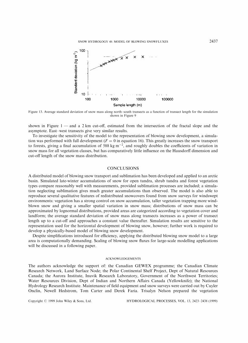
shown in Figure 1 Ð and a 2 km cut-o�, estimated from the intersection of the fractal slope and theasymptote. East±west transects give very similar results.

To investigate the sensitivity of the model to the representation of blowing snow development, a simula-tion was performed with full development (F � 0 in equation 16). This greatly increases the snow transportto forests, giving a ®nal accumulation of 588 kg mÿ2, and roughly doubles the coe�cients of variation insnow mass for all vegetation classes, but has comparatively little in¯uence on the Hausdor� dimension andcut-o� length of the snow mass distribution.

CONCLUSIONS

A distributed model of blowing snow transport and sublimation has been developed and applied to an arcticbasin. Simulated late-winter accumulations of snow for open tundra, shrub tundra and forest vegetationtypes compare reasonably well with measurements, provided sublimation processes are included; a simula-tion neglecting sublimation gives much greater accumulations than observed. The model is also able toreproduce several qualitative features of redistributed snowcovers found from snow surveys for windsweptenvironments: vegetation has a strong control on snow accumulation, taller vegetation trapping more wind-blown snow and giving a smaller spatial variation in snow mass; distributions of snow mass can beapproximated by lognormal distributions, provided areas are categorized according to vegetation cover andlandform; the average standard deviation of snow mass along transects increases as a power of transectlength up to a cut-o� and approaches a constant value thereafter. Simulation results are sensitive to therepresentation used for the horizontal development of blowing snow, however; further work is required todevelop a physically-based model of blowing snow development.

Despite simpli®cations introduced for e�ciency, applying the distributed blowing snow model to a largearea is computationally demanding. Scaling of blowing snow ¯uxes for large-scale modelling applicationswill be discussed in a following paper.

ACKNOWLEDGEMENTS

The authors acknowledge the support of: the Canadian GEWEX programme; the Canadian ClimateResearch Network, Land Surface Node; the Polar Continental Shelf Project, Dept of Natural ResourcesCanada; the Aurora Institute, Inuvik Research Laboratory, Government of the Northwest Territories;Water Resources Division, Dept of Indian and Northern A�airs Canada (Yellowknife); the NationalHydrology Research Institute. Maintenance of ®eld equipment and snow surveys were carried out by CuylerOnclin, Newell Hedstrom, Tom Carter and Derek Faria. Trisalyn Nelson prepared the vegetation

Figure 13. Average standard deviation of snow mass along north±south transects as a function of transect length for the simulationshown in Figure 9



classi®cation. Natasha Neumann provided GIS and mapping assistance. R. E. is on leave from the HadleyCentre for Climate Prediction and Research, UK Meteorological O�ce.

REFERENCES

Bintanja R. 1998. The interaction between drifting snow and atmospheric turbulence. Annals of Glaciology 26: 167±173.BioÈ schl G. 1999. Scaling issues in snow hydrology. Hydrological Processes 13: 2149±2175.DeÂ ry SJ, Taylor PA, Xiao J. 1998. The thermodynamic e�ects of sublimating blowing snow in the atmospheric boundary layer.

Boundary-Layer Meteorology 89: 251±283.Donald JR, Soulis ED, Kouwen N, Pietroniro A. 1995. A land cover-based snow cover representation for distributed hydrological

models. Water Resources Research 31: 995±1009.Goodison BE, Metcalfe JR, Louie PYT. 1998. Summary of country analyses and results, Annex 5.B Canada. In The WMO Solid

Precipitation Measurement Intercomparison Final Report, Instruments and Observing Methods Report No. 67, WMO, Geneva.Jackson PS, Hunt JCR. 1975. Turbulent wind ¯ow over a low hill. Quarterly Journal of the Royal Meteorological Society 101: 929±955.Lettau H. 1969. Note on aerodynamic roughness-parameter estimation on the basis of roughness element description. Journal of

Applied Meteorology 8: 828±832.Li L, Pomeroy JW. 1997a. Estimates of threshold wind speeds for snow transport using meteorological data. Journal of Applied

Meteorology 36: 205±213.Li L, Pomeroy JW. 1997b. Probability of occurrence of blowing snow. Journal of Geophysical Research 102: 21955±21964.Liston GE, Sturm M. 1998. A snow-transport model for complex terrain. Journal of Glaciology 44: 498±516.Mason PJ, Sykes RI. 1979. Flow over an isolated hill of moderate slope. Quarterly Journal of the Royal Meteorological Society 105:

383±395.Pomeroy JW. 1988. Wind transport of snow. Ph.D. Thesis, University of Saskatchewan.Pomeroy JW, Gray DM, Landine PG. 1993. The Prairie Blowing Snow Model: characteristics, validation, operation. Journal of

Hydrology 144: 165±192.Pomeroy JW, Gray DM. 1995. Snowcover accumulation, relocation and management. National Hydrology Research Institute Science

Report No. 7, Environment Canada, Saskatoon: 134 p.Pomeroy JW, Gray DM, Shook KR, Toth B, Essery RLH, Pietroniro A, Hedstrom N. 1998. An evaluation of snow accumulation and

ablation processes for land surface modelling. Hydrological Processes 12: 2339±2367.Pomeroy JW, Li L. 1999a. Areal snowcover mass balance using a blowing snow model. I. Model structure. Journal of Geophysical

Research. (submitted.)Pomeroy JW, Li L. 1999b. Areal snowcover mass balance using a blowing snow model. II. Application to prairie and Arctic

environments. Journal of Geophysical Research. (submitted.)Pomeroy JW, Marsh P, Gray DM. 1997. Application of a distributed blowing snow model to the Arctic. Hydrological Processes 11:

1451±1464.Raupach MR, Gillette DA, Leys JF. 1993. The e�ect of roughness elements on wind erosion threshold. Journal of Geophysical Research

98: 3023±3029.Schmidt RA. 1982. Vertical pro®les of windspeed, snow concentrations and humidity and humidity in blowing snow. Boundary-layer

Meteorology 23: 223±246.Schmidt RA. 1991. Sublimation of snow intercepted by an arti®cial conifer. Agricultural and Forest Meteorology 54: 1±27.Shook K. 1995. Simulation of the ablation of prairie snowcovers. Ph.D. Thesis, University of Saskatchewan.Shook K, Gray DM. 1996. Small-scale spatial structure of shallow snowcovers. Hydrological Processes 10: 1283±1292.Steppuhn H, Dyck GE. 1974. Estimating true basin snowcover. In Advanced concepts and techniques in the study of snow and ice

resources. National Academy of Sciences: Washington, DC.: 314±328.Takeuchi M. 1980. Vertical pro®les and horizontal increases of drift snow transport. Journal of Glaciology 26: 481±492.Taylor PA, Walmsley JL, Salmon JR. 1983. A simple model of neutrally strati®ed boundary-layer ¯ow over real terrain incorporating

wavenumber-dependent scaling. Boundary-Layer Meteorology 26: 169±189.Thorpe AD, Mason BA. 1966. The evaporation of ice spheres and ice crystals. British Journal of Applied Physics 17: 541±548.Turcotte DL. 1992. Fractals and Chaos in Geology and Geophysics. Cambridge University Press: Cambridge.Walmsley JL, Salmon JR, Taylor PA. 1982. On the application of a model of boundary-layer ¯ow over low hills to real terrain.

Boundary-Layer Meteorology 23: 17±46.Walmsley JL, Taylor PA, Keith T. 1986. A simple model of neutrally strati®ed boundary-layer ¯ow over complex terrain with surface

roughness modulations (MS3DJH/3R), Boundary-Layer Meteorology 36: 157±186.



Documents

A distributed model of blowing snow over complex terrain