A. d’Aspremont

Identifying Small Mean Reverting Portfolio

Quantitative Trading StrategiesDhanuka Rohan

Fu Xiaohang

Magnin Christophe

Sinha Prashant

Contents2

� Introduction to paper

� Enhancements

� Parameter selection

� Sparse decomposition algorithms

Greedy Search� Greedy Search

� Semi Definite Relaxation

� Our interpretation

Gist of paper and our purpose

Introduction 3

Introduction4

� Given multivariate time series, we study the problem of forming portfolios with maximum mean reversion while constraining the number of assets in these portfolios.

� We show that it can be formulated as a sparse canonical correlation analysis and study various algorithms to correlation analysis and study various algorithms to solve the corresponding sparse generalized eigenvalueproblems, specifically, greedy search and semi definite relaxation

� After discussing penalized parameter estimation procedures, we study the sparsity versus predictability tradeoff and apply the same in two markets – FX and swaps.

Introduction5

� The trading logic behind this paper is that if we confidently predict mean reversion of a basket of assets, we can then use that property to trade those assets as we have knowledge of their long term trends.

� The problem in this paper also deals with number of assets. While increasing number of assets in the basket assets. While increasing number of assets in the basket increases the mean reversion, it may reduce financial viability of trading due to complexity and cost. Thus, we want to find a solution amongst as few assets as possible.

� We thus create a asset number vs. mean reversion trade off analysis to decide optimal asset number for a given set.

Introduction6

� Once we have the assets, we can apply it to a real time trading environment and see if we can make a profit.

� We go about this task using a number of complex mathematical tools, especially in Matlab. The exact implementation is discussed next and all the code is implementation is discussed next and all the code is provided so that our implementation is immediately usable.

Introduction

� Deviation from the average price are expected to revert to the average� Sell (buy) when asset higher (lower) than average

� Classis indicator of predictability in financial markets

� Usual methods (cointegration, etc) to get mean reverting

7

� Usual methods (cointegration, etc) to get mean reverting portfolios give dense portfolios� High transaction costs

� Issues to interpret the resulting portfolios

� Goal of d’Aspremont: Finding a way to get sparse mean reverting portfolios� Given a (high) number of assets, we build a portfolio with a

few of them by maximizing predictability

What we’ve added beyond the paper

Enhancements8

Enhancements9

� The biggest issue for us was that there was low real world application to this paper, as he proves that this technique does not yield profits once transaction cost is allowed for.

� We wanted to find a way to make our efforts have real We wanted to find a way to make our efforts have real world dividends. We decided to do this by making use of Excel.

� Our purpose is to provide a trader with a black box solution where in he simply clicks a button and gets information on the mean reversion property of the assets chosen.

� He can also change the covariance matrix as per his views.

Enhancements10

� Working in a trading environment, we knew that ease of use and stability was desirable as much as final results.

� We propose a daily autosys job to run the parameter selection matlab code which uses bloomberg data and stores results in a shared drive.The trader in the day simply starts excel which can � The trader in the day simply starts excel which can import data from the share drive. Then, the trader presses calculate and gets a complete detailed picture of the mean reversion properties of different cardinality asset baskets.

� He can now use this information to support his other mean reversion trading strategies.

How to get the parameters required. Uses Matlab.

Parameter Selection11

Matlab.

Covariance Selection

� Robust and sparse estimation of the covariance matrix developed by Dempster (1972)

� Maximum-likelihood penalized by the cardinality of X

� �

12

)Card()(Trdetlogmax XXXx

ρ−∑−

� in the variable X � Sn, where � is the sample covariance matrix, Card(X) is the number of nonzero coefficients in X and �>0 controls the trade-off between log-likelihood and sparsity

� Hard to solve numerically. D’Aspremont, Banerjee & El Ghaoui (2006) replaces the penalty by the l1 norm

x

||)(Trdetlogmax1,∑

=

−∑−n

jiij

xXXX ρ

Covariance Selection – Dual Problem

Block-coordinate descent gradient method

� The dual problem is given by

� in the variable U � Sn

13

njiU

nU

ij ,,1,,||tosubject

)(detlogmin

K=≤−+∑−

ρ�

� We can decompose the matrices in blocks as follows

� where V is fixed, A � S(n-1), u,b � R(n-1) and w,c � R

� u represents the variables, i.e. the rows and columns we are updating at each iteration.

=∑

=

cb

bA

wu

uVU TT and

Covariance Selection – Dual Problem

Block-coordinate descent gradient method

� The dual problem in blocks becomes

At each iteration, the main step is then a box

14

njiuw

nubVAubcwVA

ij

T

,,1,,||,||tosubject

)]()()()log[()(detlogmin 1

K=≤≤−+++−+−+− −

ρρ

� At each iteration, the main step is then a box constrained quadratic program of the form

� can be solved using SeDuMi by Sturm (1999)

njiu

ubVAub

ij

T

,,1,,||tosubject

)()()(min 1

K=≤+++ −

ρ

Block-coordinate descent gradient method

Algorithm

� Pick the row and colum to update;

� Compute (A + V)-1;

� Update the row and column previously picked with the solution of the box constrained QP

� After each step, check the folowing convergence

15

� After each step, check the folowing convergence condition

� Matlab code available on d’Aspremont’s website

ερ ≤+−∑ ∑=

n

jiijXnX

1,

)(Tr

Covariance Selection

Example

� Each component equal to 0 in the inverse covariance matrix represents two variables that are conditionally independent� Financial meaning of the inverse covariance matrix:

idiosyncratic components of asset prices dynamics

16

� Example� 15 currencies vs. USD

� daily data from Jan 2008 to Dec 2009

� graphs done using Cytoscape

Covariance Selection

Initial inverse covariance matrix17

Covariance Selection

rho = 0.0518

Covariance Selection

rho = 0.519

A matrix

� Asset price is an autoregressive process. The second parameter to estimate is the A matrix

� where St-1 is the lagged portfolio process, A � Rnxn and Zt is a vector of Gaussian noise independent of St-1 with zero mean

� �

20

ttt ZASS += − 1

�

t-1and covariance � � Sn

� Intuitive solution: ordinary least square

� OLS estimate is used in the Box & Tiao procedure.

tTtt

Tt SSSSA 1

111 )( −

−−−=

)

Sparse A matrix

Exogeneous dependence model

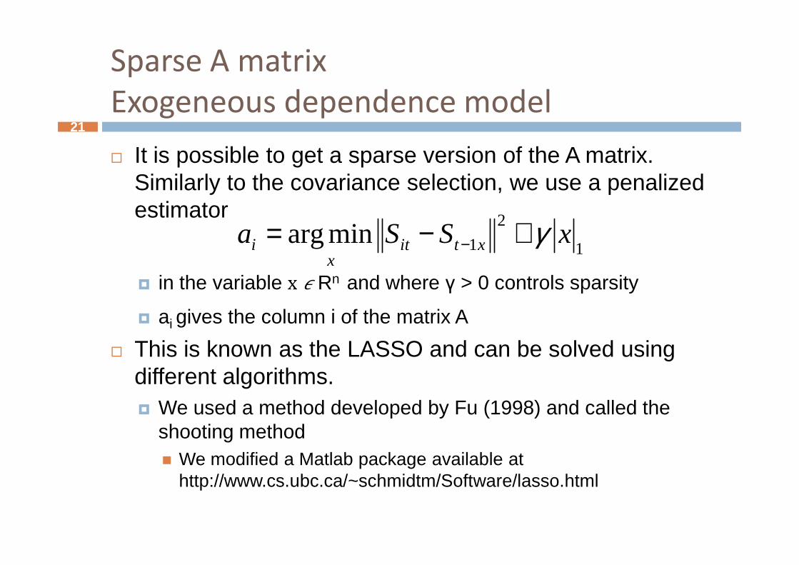
� It is possible to get a sparse version of the A matrix. Similarly to the covariance selection, we use a penalized estimator

� in the variable x � Rn and where γ > 0 controls sparsity

21

1

2

1minarg xSSa xtitx

i γ+−= −

� in the variable x � Rn and where γ > 0 controls sparsity

� ai gives the column i of the matrix A

� This is known as the LASSO and can be solved using different algorithms. � We used a method developed by Fu (1998) and called the

shooting method� We modified a Matlab package available at

http://www.cs.ubc.ca/~schmidtm/Software/lasso.html

Discussing the concepts

Sparse Decomposition Algorithms22

Sparse Decomposition Algorithms23

� The nub of this problem is to solve for a generalized eigenvalue problem which can be represented as

in the variable λ ∈ R, where A,B ∈ Sn. This is usually in the variable λ ∈ R, where A,B ∈ Sn. This is usually solved using a QZ decomposition. The largest solution of this problem can be written in variation form as:

Sparse Decomposition Algorithms24

� It is this lambda that we seek to maximize. We need to do this within certain constraints we introduce for financial reasons such as transaction cost. The main constraint we introduce is one of cardinality and finally, we solve the following

Here, is a constant greater than 0 while card(x) represents the number of non zero assets. We are basically constraining the number of assets to trade for that max lambda.

Background25

� Problem

estimating sparse mean reverting portfolios:assume portfolios follow an Ornstein-Uhlenbeck process:

with

is the value of asset at time t; Portfolio is formed by these assets with weights

ix ( )t t tdP P P dt dZλ σ= − +

1

n

t i tii

P x S=

= ∑S Pxis the value of asset at time t; Portfolio is formed by these assets with weights

� Objective

maximize mean reversion coefficientby adjusting portfolio weights

Under constraint :

cardinality of x below k.

ix1x =

tiSiS tP

ix

Sparse Decomposition Algorithms26

� As a result of canonical decomposition, we get:

� Thus, we get a model considering of the cardinality constraint:

max( , ) maxn

T

Tx R

x AxA B

x Bxλ

∈=

maximize /T Tx Ax x Bx

� Next, we discuss two techniques to get approximate solutions:

1. Greedy Search2. Semidefinite Relaxation

maximize /T Tx Ax x Bxsubject to ( )Card x k≤

1x =

Canonical Decomposition -- 127

� Assume asset prices serie follows a stationary vector autoregressive process:

measuring predictability by variance ratio:

1t t tS S A Z−= +

21tv

σ −=

� As for the portfolio, we measure predictability by

12

t

t

vσ

−=

( )T T

T

x A Axv x

x x

Γ=Γ

Canonical Decomposition -- 228

� As for the portfolio: minimizing predictability

equivalent to

finding minimum generalized eigenvalue by

det( ) 0TA AλΓ − Γ =

� Portfolio with minimum predictability is:

z is the eigenvector corresponding to the smallest eigenvalue of

A is estimated by:

det( ) 0A AλΓ − Γ =

1/ 2x z= Γ

1/ 2 1/ 2TA A− −Γ Γ Γ1

1 1 1ˆ ( )T T

t t t tA S S S S−− − −=

Implemented completely as a black box solution in Excel

Greedy Search29

solution in Excel

Greedy Search30

� The concept of greedy search is exceedingly simple and leads to a solution which might not be the most optimal but is highly cost efficient. We find the first optimal point, then the optimal point closest to it and so on.

� In this particular execution, we first find the single asset In this particular execution, we first find the single asset giving the highest mean reversion. We then fix this asset and search for the asset amongst the others such that the pair gives the highest mean reversion. In this way, we keep adding assets till k is reached.

Greedy Search31

� We start with a definition

� We now want to build recursive solutions with regards to k. We first find the initial starting point with the equation,

� We now start adding weights to assets one by one for maximum predictability as explained earlier. The equation solved is

Greedy Search32

� The cost of the solution for this implementation is O(n^4) for all k which is far more efficient than many of the deep search algorithms implemented for the problem.

� There are however some slight stability issues with this algorithm.

Also, a major issue encountered during implementation as � Also, a major issue encountered during implementation as well is that the optimal solution for the equation solved might not have an increasing support set as is assumed by the

algorithm which implements Ik⊂ Ik+1. � Thus our final answer while efficient is rarely the most optimal

and so we look at other algorithms for verification.

Implementation of Greedy Search33

� In our implementation of greedy search, we wanted to find a more trader or front office friendly solution, especially as this was the simpler of the two algorithms.

� We thus decided to use Excel and VBA coding for our final solution. Our concept is that we can calculate the final solution. Our concept is that we can calculate the matrices using Matlab as a singular package and store them in a library.

� Then, at any point, the trader could import the data, modify as required and by simply clicking one macro, he would get the optimal weights with associated mean reversions, allowing him to take a call.

Implementation of Greedy Search34

� Using this method, this paper becomes more useful as it provides a weighted and fundamental research into asset mean reversion and allows the traders to make real time calls.

� The reason we did this was using only d’Aspremont’smethod, we found that there is no profit being generated after method, we found that there is no profit being generated after including transaction cost. We then searched for a way to make this ore useful for the final user and came up with this.

� For excel execution, we use the Matrix functions inbuilt in excel and extensively use the Solver with constraints as specified to generate the final values. It fundamentally follows the greedy search algorithm in all aspects.

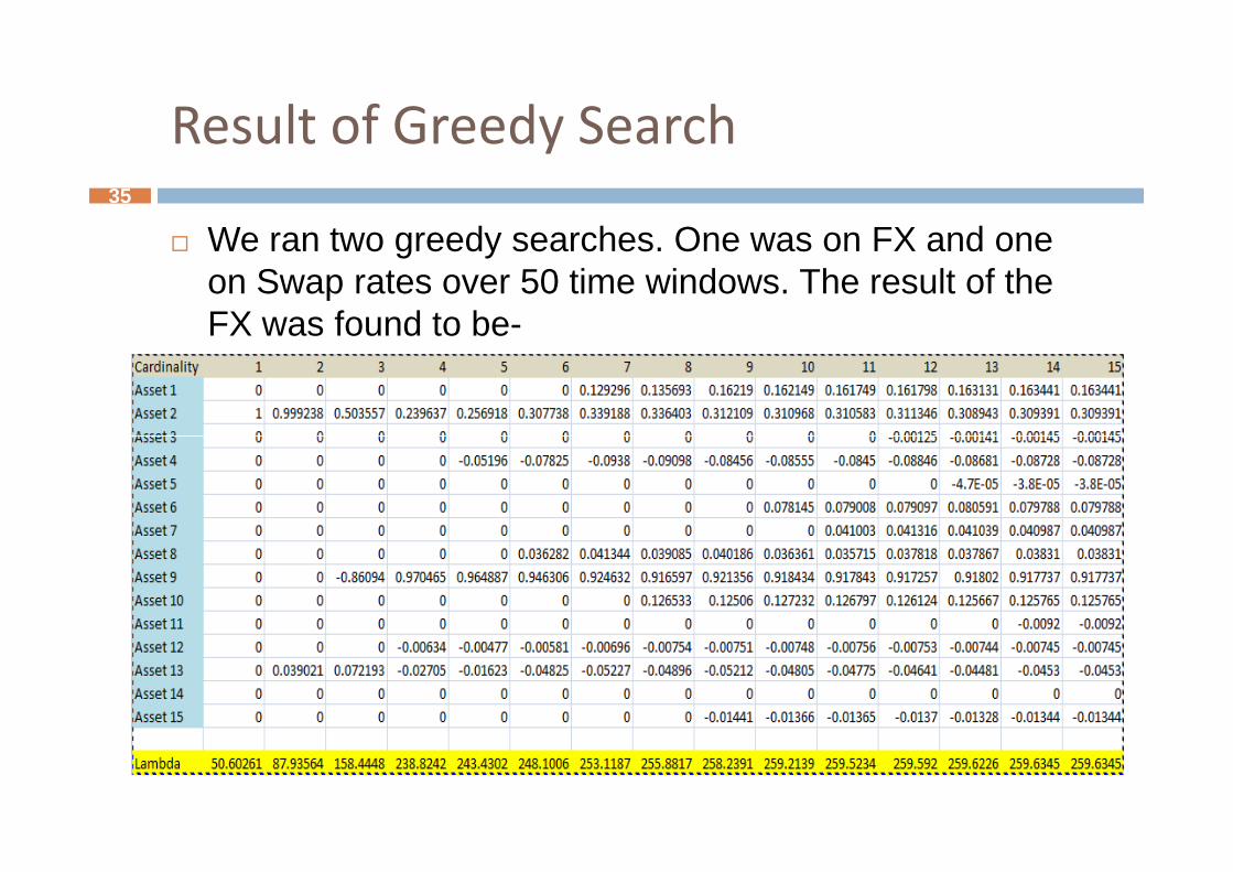
Result of Greedy Search35

� We ran two greedy searches. One was on FX and one on Swap rates over 50 time windows. The result of the FX was found to be-

36

200

250

300

Mean

R

FX

Results of Greedy Search

0

50

100

150

1 2 3 4 5 6 7 8 9 10 11 12 13 14 15

eversion

Cardinality

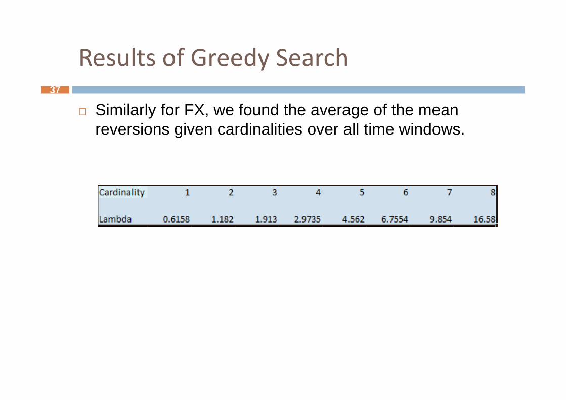
Results of Greedy Search37

� Similarly for FX, we found the average of the mean reversions given cardinalities over all time windows.

Results of Greedy Search38

10

12

14

16

18

Mean

Re

Swap

0

2

4

6

8

1 2 3 4 5 6 7 8

eversion

Cardinality

Lambda

Complete implementation in Matlab

Semi Definite Relaxation39

Semidefinite Relaxation -- 140

� Formulate a semidefinite relaxation for sparse generalized eigenvale problems:

subject to Rank(X) 1=x =1

T Tmaximize x A x/ B xx

� Equivalent problem (let ):

nwith x R∈

maximize Tr(AX)/Tr(BX)2subject to Card(X) k≤

Tr( ) 1X =

X 0f

Rank(X) 1=

T nX xx S= ∈

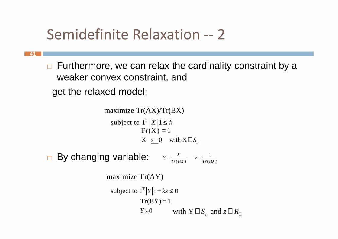
Semidefinite Relaxation -- 241

� Furthermore, we can relax the cardinality constraint by a weaker convex constraint, and

get the relaxed model:

maximize Tr(AX)/Tr(BX)Tsubject to 1 1X k≤

� By changing variable:

Tsubject to 1 1X k≤T r(X ) 1=X 0f

( )

XY

Tr BX= 1

( )z

Tr BX=

maximize Tr(AY)

Tsubject to 1 1 0Y kz− ≤Tr(BY) 1=

0Yf

with X nS∈

with Y and nS z R+∈ ∈

Semidefinite Relaxation

Results for Swap rate Data42

250

300

350

lambda vs k

0

50

100

150

200

0 2 4 6 8 10

lambda vs k

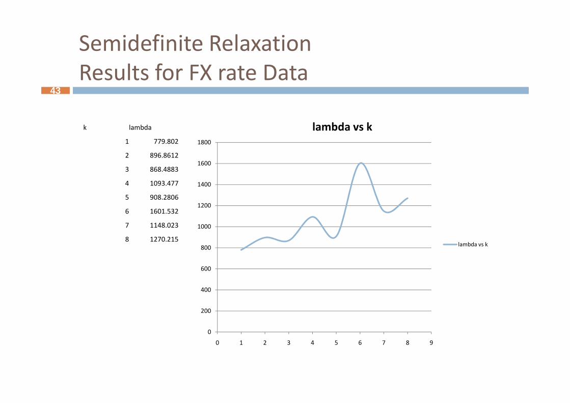
Semidefinite Relaxation

Results for FX rate Data43

1200

1400

1600

1800

lambda vs kk lambda

1 779.802

2 896.8612

3 868.4883

4 1093.477

5 908.2806

0

200

400

600

800

1000

1200

0 1 2 3 4 5 6 7 8 9

lambda vs k

5 908.2806

6 1601.532

7 1148.023

8 1270.215

Our interpretation of the entire project

Intepretation44

Interpretation45

� We were impressed with the mathematical rigor of the paper and the strong techniques used to implement it. However, we were slightly unhappy with the end result.

� As in the paper, the final results are not strong enough to be used as a all in trading technique. What we instead to be used as a all in trading technique. What we instead propose is to simplify the execution of this process and use it as a fundamental analysis tool to help support the trader’s decision making

� Greedy search was found to be almost as good at interpretation as the much more costlier semi definite relaxation

Interpretation46

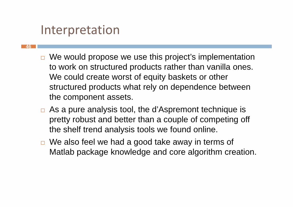
� We would propose we use this project’s implementation to work on structured products rather than vanilla ones. We could create worst of equity baskets or other structured products what rely on dependence between the component assets.

� As a pure analysis tool, the d’Aspremont technique is pretty robust and better than a couple of competing off the shelf trend analysis tools we found online.

� We also feel we had a good take away in terms of Matlab package knowledge and core algorithm creation.

References

� Banerjee O., El Ghaoui L., d’Aspremont A., Model Selection through Sparse Maximum Likelihood Estimation, Journal of Machine Learning Research, pp. 485-516, March 2008

� d’Aspremont A., Identifying Small Mean Reverting

47

d’Aspremont A., Identifying Small Mean Reverting Portfolios, Quantitative Finance, pp. 351-364, March 2011

� Fu W. J., Penalized Regressions: The bridge versus the Lasso, Journal of Computational and Graphical Statistics, pp. 397-416, September 1998