A Cutting Plane Method for Solving Linear Generalized ...egon.cheme.cmu.edu/Papers/SawayaGrossmann.pdfA Cutting Plane Method for Solving Linear Generalized Disjunctive Programming

A Cutting Plane Method for Solving Linear Generalized

Disjunctive Programming Problems

Nicolas W. Sawaya and Ignacio E. Grossmann1

Department of Chemical Engineering, Carnegie Mellon University, Pittsburgh, PA, 15213 USA

April 2004

Abstract: Raman and Grossmann (1994) and Lee and Grossmann (2000) have developed a

reformulation of Generalized Disjunctive Programming (GDP) problems that is based on

determining the convex hull of each disjunction. Although the relaxation of the reformulated

problem using this method will often produce a significantly tighter lower bound when

compared with the traditional big-M reformulation, the limitation of this method is that the

representation of the convex hull of every disjunction requires the introduction of new

disaggregated variables and additional constraints that can greatly increase the size of the

problem. In order to circumvent this issue, a cutting plane method that can be applied to linear

GDP problems is proposed in this paper. The method relies on converting the GDP problem

into an equivalent big-M reformulation that is successively strengthened by cuts generated

from an LP or QP separation problem. The sequence of problems is repeatedly solved, either

until the optimal integer solution is found, or else until there is no improvement within a

specified tolerance, in which case one switches to a branch and bound method. The strip-

packing, retrofit planning and zero-wait job shop scheduling problems are presented as

examples to illustrate the performance of the proposed cutting plane method.

Keywords: MIP, Disjunctive Programming, cutting planes, strip-packing, retrofit planning,

job-shop scheduling

1. INTRODUCTION

The most commonly used model in discrete/continuous optimization corresponds to a

Mixed Integer Non Linear Program (MINLP). More recently, however, Generalized

Disjunctive Programming (GDP), which is a generalization of disjunctive programming

1 Author to whom correspondence should be addressed

1

(Balas, 1998), has been proposed by Raman and Grossmann (1994) as an alternative model to

the MINLP problem (Grossmann, 2002, Tawarmalani and Sahinidis, 2002). While the MINLP

model is based entirely on algebraic equations and inequalities, the GDP model allows a

combination of algebraic and logical equations through disjunctions and logic propositions,

which facilitates the representation of discrete decisions. Furthermore, Lee and Grossmann

(2000) have shown that any GDP model can be converted into an equivalent MINLP

reformulation. Currently, there are several algorithms and different approaches in the literature

to tackle GDP problems (Grossmann, 2002), though some perform inefficiently under certain

conditions and for certain classes of problems. We are thus interested in developing novel

algorithms and solution methods aimed at solving both linear and non-linear GDP problems

more efficiently, although we restrict ourselves exclusively to the linear case in this paper.

Lee and Grossmann (2000) have proposed a reformulation to solve convex nonlinear

GDP problems with multiple disjunctions based on determining the convex hull of each

disjunction. Although the feasible region of the reformulated problem does not correspond to

the true convex hull of the problem, we nonetheless have termed that reformulation in this

paper as the “convex hull” reformulation for the sake of convenience. There exists other GDP

to MINLP reformulations of which the traditional big-M reformulation is the most common.

Grossmann and Lee (2003) have shown that the feasible region of the relaxation resulting from

the convex hull reformulation projected onto the space of the big-M reformulation is always as

tight as, or tighter than that of the big-M reformulation. The tightness of the relaxed feasible

region, which is usually reflected in the lower bound of the problem (for minimization), is an

important criterion when solving the original Mixed Integer Program, as tighter relaxed

feasible regions reduce the search space of the solution algorithm. However, the representation

of the convex hull requires the introduction of new disaggregated variables and additional

constraints that can greatly increase the size of the problem, thus limiting the effectiveness of

the method.

In order to circumvent the aforementioned problem, we present in this paper a cutting

plane method that exploits the potentially tighter convex hull relaxed feasible region without

the additional constraints and variables. This method can be applied to linear GDP problems

that correspond to MIP problems, or else to master problems that are used in the solution of

nonlinear GDP problems (Turkay and Grossmann, 1996). We present the strip-packing,

retrofit planning and zero-wait job shop scheduling problems to illustrate the computational

2

performance of the proposed method in solving these problems and compare all results

obtained to those using the convex hull and big-M reformulations.

2. BACKGROUND

Consider the linear generalized disjunctive programming problem (LGDP), which is based

on the work of Raman and Grossmann (1994) and is an extension of the work of Balas (1998):

1

. .

( )0 , , , ,

jk

k

Tk

k K

jk jkj J

k j k

k jk k

Min Z c d x

s t Bx b

Y

A x a k K

c

Y Truex U c Y True False j J k K

γ

∀ ∈

∀ ∈

+

= +

≤

⎡ ⎤⎢ ⎥

≤ ∀ ∈⎢ ⎥⎢ ⎥=⎣ ⎦

Ω =

≤ ≤ ∈ ∈ ∀ ∈ ∀ ∈

∑

∨

R

(LGDP)

Here, x is a vector of continuous variables bounded by a vector of upper bounds U,

jkY are Boolean variables, 1kc +∈ R are continuous variables that represent the cost associated

with each disjunction and jkγ are fixed charges. A disjunction k K∈ is composed of several

disjuncts j ∈ Jk, each containing a set of linear equations and/or inequalities ( jk jkA x a≤ )

representing the constraints of the problem, connected together by the logical OR operator (∨)

that enforces the contents of only one disjunct. Discrete decisions are represented by the

Boolean variables jkY in terms of disjunctions k K∈ and logic propositions ( )YΩ that are

assumed to be expressed in Conjunctive Normal Form (CNF). Thus, only the constraints inside

disjunct j ∈ Jk where jkY is true are enforced; otherwise, the corresponding constraints are not

enforced. Finally, Bx b≤ are common constraints that must hold regardless of the discrete

decisions that are selected.

The linear GDP problem (LGDP) can be reformulated as a Mixed Integer Program

(MIP) in different ways, including the two most common alternatives termed big-M (BM) and

convex hull reformulations (CH). In order to obtain the big-M reformulation, problem LGDP

is transformed into an MIP by replacing the Boolean variables jkY by binary variables jky and

3

using big-M constraints. The logic constraints ( )YΩ are converted into linear inequalities

(Williams, 1985), which leads to the following reformulation (Raman and Grossmann, 1994):

. . (1 ) ,

1

, ,

k

k

Tjk jk

k K j J

jk jk jk jk k

jkj J

njk k

Min Z y d x

s t Bx bA x a M y j J k K

y k K

Dy dx y j J k K

γ∀ ∈ ∀ ∈

∀ ∈

+

= +

≤− ≤ − ∀ ∈ ∀ ∈

= ∀ ∈

≤

∈ ∈0,1 ∀ ∈ ∀ ∈

∑ ∑

∑

R

(BM)

Here, jkM are the “big-M” parameters that render the jth system of inequalities in the

kth disjunction redundant when jky = 0 (i.e. jkY = False). The inequalities Dy d≤ can be

systematically derived from their logical CNF form ( )YΩ as discussed by Williams (1985),

Raman and Grossmann (1994), and Hooker (2000).

In order to obtain the convex hull reformulation (CH), problem LGDP is transformed

into an MIP by replacing the Boolean variables jkY by binary variables jky and disaggregating

the continuous variables nx +∈ R into new variables nν +∈ R . Using the convex hull

constraints for each disjunction (Balas, 1998; Raman and Grossmann, 1994), this leads to the

following reformulation (Raman and Grossmann, 1994):

. . ,

,

k

k

Tjk jk

k K j J

jk jk jk jk k

jkj J

jk jk jk k

Min Z y d x

s t Bx bA a y j J k K

x k K

y U j J k K

y

γ

ν

ν

ν

∀ ∈ ∀ ∈

∀ ∈

= +

≤≤ ∀ ∈ ∀ ∈

= ∀ ∈

≤ ∀ ∈ ∀ ∈

∑ ∑

∑

1

, , ,

k

jkj J

njk k

k K

Dy dx y j J k Kν

∀ ∈

+

= ∀ ∈

≤

∈ ∈0,1 ∀ ∈ ∀ ∈

∑

R

(CH)

4

The new variables nν +∈ R in (CH) are the disaggregated variables, while the

parameters jkU serve as their upper bounds. The latter are usually chosen so as to match the

upper bounds on the continuous variables nx +∈ R . Note that ( jky = 0) ⇒ ( jkν = 0), and thus

the jth system of inequalities in the kth disjunction is redundant.

In comparing the reformulations in (BM) and (CH), the following trade-offs can be

observed. On the one hand, the relaxed feasible region of the (CH) reformulation is at least as

tight, if not tighter, than that of the (BM) reformulation (see Fig. 1). This is reflected in the

lower bounds of the aforementioned reformulations, where the lower bound of the relaxation

of (CH) is equal to or greater than the lower bound of the relaxation of problem (BM), as has

been proven by Grossmann and Lee (2003). The tightness of the feasible region, and by

extension, the quality of the lower bound, affects the number of nodes being examined within

the framework of a B&B algorithm. Thus a tighter feasible region, and by extension, a tighter

lower bound, leads to a reduction in the search space of a particular problem, which usually

translates into faster solution times. The example in Figure 1 illustrates in the (x,y) space the

convex hull and big-M relaxations of the single disjunction [ ] [ ]3210 ≤≤∨≤≤ xx that is

expressed in terms of the Boolean variable Y to indicate whether the first term (Y=False) or

second term (Y=True) applies. In this case, it is clear that the convex hull relaxation is tighter

than the big-M relaxation, despite the optimal value of M having been chosen (M=3).

Figure 1. Comparison between (BM) and (CH) relaxed feasible regions

(BM) Relaxed Feasible Region

(CH) Relaxed Projected Feasible Region

x

y

0 1Yx

¬⎡ ⎤⎢ ⎥≤ ≤⎣ ⎦

2 3Yx

⎡ ⎤⎢ ⎥≤ ≤⎣ ⎦

1

1 2 3

5

On the other hand, the size of the (CH) reformulation is considerably larger than the

size of the (BM) reformulation, which leads to an increase in solution time required per

iteration at every node, and furthermore, to an increase in the number of total iterations per

node. Hence, in general, it is very difficult to determine a priori when a given reformulation

will be more effective than the other one in solving the problem (Vecchietti et al., 2003).

Therefore, it would appear that a desirable objective is to develop a method for generating

cutting planes from the (CH) relaxation in order to strengthen the looser but smaller (BM)

reformulation. In this fashion, one takes advantage of the tighter (CH) reformulation without

incurring an increase in the number of variables and a significant increase in the number of

constraints in the problem. Such an idea is proposed in the following section.

3. CUTTING PLANE METHOD

The basic idea of the proposed cutting plane method consists in solving a sequence of

relaxed big-M MILPs with cutting planes that are successively generated from the convex hull

relaxation projected onto the (x,y) space. More specifically, the cutting planes are determined

by solving an LP (or QP) separation problem, whose feasible region corresponds to that of the

convex hull relaxed reformulation. The separation problem has, as an objective, to find a point

within the convex hull relaxed feasible region “closest” to the optimal solution point yielded

by the relaxed big-M MILP. In essence, the objective of the separation problem consists of

finding a cutting plane that corresponds to the most violated constraint of the convex hull that

is projected onto the space of the original variables of the big-M MILP. A repeating sequence

of relaxed big-M MILPs (with cuts up to that point) and LP (or NLP) separation problems

yielding new cuts is iteratively solved until the optimal solution for the original MILP is found

or until there is no improvement within a specified tolerance ε, in which case one switches to a

B&B method for solving the resulting big-M MILP with all the cutting planes that have been

generated.

It is interesting to note that the proposed cuts, though related to a certain extent to some

of the work done on lift-and-project cutting planes originally developed by Balas, Ceria and

Cornuejols (1993), are different in important ways from the latter. The major distinction lies in

the derivation and generation of our cuts, which are crucially based on a GDP formulation, as

opposed to a 0-1 MIP formulation, as in the case of lift-and-project cuts. Furthermore, if we

6

were to contextualize their work within a GDP framework, lift-and-project cuts would be

generated through a sequential convexification procedure that would obtain by taking the

convex hull of one disjunction at a time, as opposed to our proposed method which generates

cuts based on a formulation that considers the intersection of the convex hulls of every

disjunction. Thus, the elementary closure resulting from our cuts is not equivalent to that of

lift-and-project cuts, since the latter’s closure corresponds to the true convex hull of the

original problem, as opposed to our case, where the elementary closure corresponds to the

feasible region arising from the aforementioned strengthened formulation that considers all

disjunctions simultaneously. We plan on comparing our cuts, both theoretically and

computationally, to other cuts present in the literature, including lift-and-project cuts, mixed-

integer Gomory cuts and mixed-integer rounding cuts, amongst others in a subsequent paper.

3.1 Separation Problem

The general form of the separation problem (SEP) is as follows (see Stubbs and

Mehrotra, 1999; Vecchietti et al., 2003):

( ) || ||. .

,

k

bm

jk jk jk jk k

jkj J

jk jk j

Min z z zs t Bx bA a y j J k K

x k K

y U

φ

ν

ν

ν∀ ∈

= −≤

≤ ∀ ∈ ∀ ∈

= ∀ ∈

≤

∑ , (SEP)

1

,

k

k k

jkj J

j J k K

y k K

Dy d

x ν

∀ ∈

∀ ∈ ∀ ∈

= ∀ ∈

≤

∑

| |

, [ , ] ,0 ,k

k K

Jn n

jk kz x y y j J k K∀ ∈+ + +

∑∈ ≡ ∈ × ≤ ≤ 1 ∀ ∈ ∀ ∈R R R

The objective function ( )zφ corresponds to determining the point | |k

k K

Jnz ∀ ∈

+ +

∑∈ ×R R

within the convex hull relaxation “closest” to the point bmz , which corresponds to the optimal

solution of the relaxed big-M MILP. In order to represent distance in the function ( )zφ ,

the 1-norm 1( ) || || | |bm bmi i

i

z z z z zφ = − ≡ −∑ ,

7

the Euclidean norm 1/ 2

2( ) || || ( ) ( )bm bm T bmz z z z z z zφ ⎡ ⎤= − ≡ − −⎣ ⎦ ,

or the infinity norm, ( ) || || max | |bm bmi i iz z z z zφ ∞= − ≡ − can be used. If either the 1-norm or

the ∞-norm is used, then the separation problem is an LP; otherwise, using the Euclidean norm

yields a QP.

3.2 Derivation of Cutting Planes

In this section, we present the derivation of the proposed cutting planes that are

obtained from the separation problem (SEP). The proofs of the propositions presented can be

found in Appendix A.

The first proposition formalizes the observation in Figure 1 that the feasible region of the

separation problem (SEP), which corresponds to that of the convex hull reformulation, is

contained within the feasible region of problem (BM).

Proposition 1: Let (FR-SEP) be the feasible region of the separation problem (SEP) in the

(z,ν) space, and let (FRP-SEP) represent the projection of (FR-SEP) onto the z-space. Then,

(FRP-SEP) ⊆ (FR-BM), where (FR-BM) represents the feasible region of (BM) in the z-space.

Furthermore, (FRP-SEP) is a convex set.

The second proposition provides the general form of the valid inequality that corresponds to

the cutting plane that is determined from the separation problem (SEP).

Proposition 2: Let bmz be the optimal solution of (BM) and sepz be an optimal solution to

(SEP). If bmz ∉ (FRP-SEP), then ∃ ξ such that ( ) 0T sepz zξ − ≥ is a valid linear inequality in

z that cuts away bmz , and such that ξ is a subgradient of ( )zφ at sepz , where ( )zφ

corresponds to the objective function of (SEP).

Using the example previously shown in Figure 1, Figure 2 demonstrates how the proposed cut

( ) 0T sepz zξ − ≥ cuts away bmz and slices off part of the feasible region of problem (BM), thus

8

strengthening the formulation. Also, note that the cut generated in this case corresponds to a

facet of the feasible region of problem (SEP).

Figure 2. Graphical representation of proposition 2

The third proposition shows that the subgradient of a differentiable function at a specific point

corresponds to the gradient of the function at that same point.

Proposition 3: Let (FRP-SEP) ⊂ S, where S is a convex set. If : Sφ → R is differentiable over

its entire domain, then the collection of subgradients of φ at sepz is the singleton set

| ( )sep sep sep sepzφ ξ ξ φ∂ ≡ = ∇ , which corresponds to the gradient of φ at sepz .

The last two propositions provide the specific expressions for the subgradient ξ in the

inequality ( ) 0T sepz zξ − ≥ for the Euclidean and ∞-norms, respectively. It should be noted that

for the case of the 1-norm, the treatment is entirely similar as the ∞-norm.

Proposition 4: Let (FRP-SEP) ⊂ S, where S is a convex set. If : Sφ → R is defined as 2

2( ) || ||bmz z zφ = − , then the collection of subgradients of φ at sepz is the singleton set

| 2( )sep sep sep sep bmz zφ ξ ξ∂ ≡ = − .

(BM) Strengthened Relaxed Feasible Region

x

y

zbm

Cutting Plane ( ) 0T sepz zξ − ≥

zsep


1

12 3

(SEP) Relaxed Projected Feasible Region

9

Proposition 5: Let (FRP-SEP) ⊂ S, where S is a convex set. If : Sφ → R is defined as

( ) || ||bmz z zφ ∞= − , then the collection of subgradients of φ at sepz is the set:

[ ]sep sep sep sep sepφ ξ ξ µ µ+ −∂ ≡ = − ,

where sepµ+ and sepµ− correspond to the optimal Lagrange multipliers of constraints (1) and

(2) respectively, in the following problem (SEP2):

1 2

. . (1)

(2)

bmi ibm

i i

Min us t u z z i M

u z z i M

R z R rν

≥ − ∀ ∈

≥ − ∀ ∈

+ ≤

The cutting planes generated by the proposed method and based on propositions 2, 4

and 5 can be used at the root node of the branch and bound tree in order to strengthen the

corresponding relaxation of problem (BM). It is, of course, generally not obvious which of the

different norms provides the deepest cut, as this is usually problem dependent. Furthermore,

the depth of the cut will be affected, particularly in the cases of the 1-norm and the ∞-norm, by

the selection of a specific set of (non-unique) optimal Lagrange multipliers, which is usually

solver dependent. The following example provides a geometrical interpretation of the three

different cuts when applied to the example in Figure 1.

1

2 31

Yx

c

⎡ ⎤⎢ ⎥≤ ≤⎢ ⎥⎢ ⎥=⎣ ⎦

Max Z = x – (c1+c2)

∨2

0 10

Yx

c

⎡ ⎤¬⎢ ⎥≤ ≤⎢ ⎥⎢ ⎥=⎣ ⎦

s.t.

10

Figure 3. Cutting plane generated when Euclidean or Infinity norm are used in (SEP)

Figure 4. Cutting plane(s) generated when 1-norm is used in (SEP)

In Figure 3, the cut generated when the Euclidean norm or Infinity norm is used

corresponds to a facet of the convex hull of the disjunction. However, in Figure 4 where the 1-

norm is used, there is an infinite set of cutting planes that can be generated since the set of

Lagrange multipliers corresponding to the optimal solution sepz is not unique. Clearly then, the

“quality” and depth of the cut generated from our procedure depends on the norm used in the


x

y

zbm

Cutting Plane ( ) 0T sepz zξ − ≥

z2sep


1

12 3

zinfsep


z1sep

Possible Cutting Planes



x

y

zbm


11

separation problem. The difference in quality and depth of the cuts resulting from the use of

different norms in the separation problem will be examined in more detail and rigour in a

subsequent paper.

3.3 Cutting Plane Algorithm

Given the propositions of the previous section, the steps of the proposed algorithm are

as follows:

0) Specify a tolerance ε for the norm of the distance in the separation problem (SEP). Set

n= 0, where n represents the iteration index.

1) Solve the continuous relaxation of (BM)n termed (RBM)n, which corresponds to the

following problem. This yields the point , ,[ , ]bm n bm nz x y≡ .

,

. . (1 ) ,

1

( ) 0 1, 2... 1

k

k

Tjk jk

k K j J

jk jk jk jk k

jkj J

lT sep l

n

Min Z y d x

s t Bx bA x a M y j J k K

y k K

Dy dz z l n

x

γ

ξ

∀ ∈ ∀ ∈

∀ ∈

+

= +

≤− ≤ − ∀ ∈ ∀ ∈

= ∀ ∈

≤

− ≥ = −

∈

∑ ∑

∑

R| |

, 0 1 ,

[ , ]k

k K

jk k

Jn

y j J k K

z x y ∀ ∈+ +

≤ ≤ ∀ ∈ ∀ ∈

∑≡ ∈ ×R R

(RBM)n

2) Solve the separation problem (SEP)n, which corresponds to the following problem.

This yields the point , ,[ , ]sep l sep lz x y≡ .

12

, ( ) || ||. .

,

k

bm n

jk jk jk jk k

jkj J

jk j

Min z z zs t Bx bA a y j J k K

x k K

y

φ

ν

ν

ν∀ ∈

= −≤

≤ ∀ ∈ ∀ ∈

= ∀ ∈

≤

∑n , (SEP)

1 k

k jk k

jkj J

U j J k K

y k K

Dy∀ ∈

∀ ∈ ∀ ∈

= ∀ ∈

≤

∑

| |

, , [ , ] ,0 ,k

k KJ

n njk k

d

x z x y y j J k Kν ∀ ∈+ + +

∑∈ ≡ ∈ × ≤ ≤1 ∀ ∈ ∀ ∈R R R

a) If ,( ) || || bm nz z zφ ε= − ≤ , then stop, and proceed to the LP-based branch-and-bound

solution of problem (BM)n with all the added cutting planes.

b) Else, generate cutting plane ,( ) 0lT sep lz zξ − ≥ , and add to (RBM)n,. Set n=n+1, go to 1.

The effectiveness of the above algorithm is dependent on the tradeoff between the

amount of time spent on the cut generation procedure versus the amount of time “saved” in the

B&B tree relative to either the big-M formulation without cuts, or to the convex hull

formulation. In the former case, these savings usually result from a tightening of the relatively

loose big-M feasible region, while in the latter case, these savings result from the smaller

number of variables and constraints in the big-M plus cuts formulation. The cut generation

procedure involves solving a sequence of separation problems (SEP)n that are LPs or QPs, so

it can be expected that it will take a reasonable amount of time to solve these problems in order

to generate the proposed cuts. It is important to note that the feasible region of the

strengthened big-M problem will be, at the very best, as tight as that of the convex hull

formulation, and thus, intuitively at least, lead us to believe that the cut generation procedure is

finite. In other words, no further cuts will be generated either when the optimal point of

(RBM)n lies within the feasible region of (SEP)n, or when the feasible region of the

strengthened big-M problem is exactly equivalent to that of (SEP)n. A rigorous proof of the

previous claim will be performed in a subsequent paper. The question that remains, however,

is whether these cuts are effective enough in slicing off parts of the big-M feasible region that

are superfluous. This is examined in detail in the next section, and we apply the above

13

algorithm to three different problems that highlight some of the major strengths and

weaknesses of the proposed method.

4. NUMERICAL RESULTS

In this section, we present the results of the proposed cutting plane algorithm on the

strip-packing, retrofit planning and zero-wait job shop scheduling problems. The strip-packing

problem is an example within a class of problems suitably solved by the proposed method,

while the last two problems serve to highlight an important characteristic regarding the

usefulness of the method, notably the degree of tightness exhibited by the convex hull

relaxation.

We present results for the strip-packing problem using the proposed method with all

norms, although the discussion is mostly focused on results obtained using the infinity norm as

the latter turned out to be the most efficient norm. This observation also holds true for the

retrofit planning and zero-wait job shop scheduling problems, thus we only present and discuss

results obtained using the infinity norm. All results obtained using the proposed cutting plane

method are discussed and compared with those obtained using the aforementioned convex hull

and big-M reformulations, where optimal values of the big-M parameters were used (i.e. equal

to ( )jk jkxmax A x a− ).

All example problems were solved with GAMS (Brooke, Kendrick, Meeraus and

Raman, 1997) on a 2.8 GHz Pentium IV PC (512 MB of RAM). The CPLEX solver (v. 8.1)

was used for the infinity norm for all three problems and for all comparisons between

reformulations with all MIP options turned off and with default options turned on, while the

CPLEX solver (v. 9.0) was used for the 1-norm and Euclidean norm. Note that the LP pre-

solver was turned off during the cut-generation procedure for reasons of computational

efficiency. Finally, the cuts generated are added only at the root node of the B&B tree.

4.1 Strip-Packing Problem

Cutting and Packing problems belong to a well known family of combinatorial NP-

Hard optimization problems that arise in numerous applications of computer science, industrial

engineering and operations management (Hifi, 1998). One important problem in this family is

the strip-packing problem, where a given set of small rectangles is packed into a strip of fixed

14

width W but unknown length L. The aim is to minimize the length of the strip while fitting all

rectangles without any overlap and without rotation. We propose the following general linear

GDP model for problem (SP-GDP):

(1)

. . i i

Min lts t lt x L≥ +

1 2 3 4

(2)

, , (3)

ij ij ij ij

i i j j j i i i j j j i

i i i

i N

Y Y Y Yi j N i j

x L x x L x y H y y H y

x UB L

∀ ∈

⎡ ⎤ ⎡ ⎤ ⎡ ⎤ ⎡ ⎤∨ ∨ ∨ ∀ ∈ <⎢ ⎥ ⎢ ⎥ ⎢ ⎥ ⎢ ⎥

+ ≤ + ≤ − ≥ − ≥⎢ ⎥ ⎢ ⎥ ⎢ ⎥ ⎢ ⎥⎣ ⎦ ⎣ ⎦ ⎣ ⎦ ⎣ ⎦≤ − (4)

i i

i NH y W

∀ ∈≤ ≤

1 1 2 3 4

(5)

, , , , , , , , , i i ij ij ij ij

i N

lt x y Y Y Y Y True False i j N i j+

∀ ∈

∈ ∈ ∀ ∈ <R

The objective in this problem consists of minimizing the length of the strip lt (1) and

(2) by representing every rectangle by its coordinates in the (x,y) space such that no overlap

occurs between rectangles. Thus, every rectangle i∈N has length Li, height Hi and coordinates

(xi, yi), where the point of reference corresponds to the upper left corner of every rectangle. By

constraining every pair of rectangles (i,j) where (i,j ∈ N, i < j) such that no overlap occurs, we

obtain a series of disjunctions with four disjuncts each, where each disjunct represents the

position of rectangle i in relation to rectangle j (3). Note that the y-coordinate of every

rectangle is bounded from above by the fixed width of the strip W (5), and that the upper

bound UBi, which in a best case scenario would correspond to the optimal value of lt, is

obtained using a bottom-left rectangle-placing heuristic and serves as an upper bound for the x-

coordinate of every rectangle (4).

We consider first a twelve-rectangle instance of the strip-packing problem (SP-GDP)

with the following ordered lengths and heights for every rectangle: (1,10), (2,9), (3,8), (4,4),

(5,5), (9,6), (7,7), (6,3), (5,2), (12,1), (3,1), (2,3). The problem was transformed into an MIP

model by using both the big-M and convex hull reformulations that are given in Appendix B.

The problem sizes for both reformulations are listed in Table 1, and the graphical solution to

this problem is presented in Figure 5.

15

Table 1. Problem sizes for 12-rectangle strip-packing problem Total number of constraints Total number of variables Number of discrete variables

Convex Hull 1663 1346 264 Big-M 343 290 264

Figure 5. Graphical Solution for 12-rectangle strip-packing problem

We also solved the problem using the cutting plane method with the infinity norm, and

compared the resulting solutions to those from the convex hull and big-M reformulations in

Tables 2 and 3. We first examine the results with all MIP algorithmic options turned off (see

Table 2). This is done in order to better gauge the effect of the proposed cuts on solution time

and number of nodes examined during the B&B procedure:

Table 2. Results for 12-rectangle strip-packing problem (∞-norm, MIP options off)

Relaxation Optimal Solution

Gap (%)

Total Nodes in MIP

Solution Time for Cut

Generation (sec)

*Total Solution Time

(sec)

Number of Nodes per sec

Convex Hull 12 27 55.55 682 464 0 1 286.39 530.52 Big-M 12 --- --- 54 244 296 0 >10 800 5022.36

Big-M + 40 cuts 12 --- --- 41 831 856 2.44 >10 800 3873.32 Big-M + 50 cuts 12 27 55.55 10 289 250 3.05 2 986.33 3 448.97 Big-M + 60 cuts 12 27 55.55 694 596 3.66 191.95 3 688.96 Big-M + 70 cuts 12 27 55.55 320 535 4.27 97.61 3 434.05 Big-M + 80 cuts 12 27 55.55 502 727 4.88 154.23 3 366.09 Big-M + 87 cuts 12 27 55.55 72 677 5.31 27.51 3 273.73

* Total solution time includes times for relaxed MIP(s) + LP(s) from separation problem + MIP

The optimal solution of the problem is 27. The lower bound obtained from the

relaxation is equal to 12 for both (BM) and (CH) reformulations, but the problem was solved

in 682 464 nodes using the (CH) reformulation, as opposed to the big-M reformulation, which

failed to solve the problem after 54 244 296 nodes. This is due to the tighter relaxed feasible

2 4

7

12

6

10

y

x Optimal Length: 27

1

3

5

8

9

10 11

16

region of (CH) when compared to that of (BM), which results in substantial savings in

computational time (1286.39 sec vs. > 10800 sec). Note however that the LP at every node of

the (CH) B&B tree is about 10 times more expensive to solve than that of the (BM)

reformulation as seen by the amount of nodes computed per sec for both reformulations

(530.52 vs. 5022.36). This is due to the larger number of variables and constraints present in

the (CH) reformulation. After the addition of 50 cutting planes to the (BM) reformulation, we

are able to solve the problem in less than the self imposed limit of three hours (2986.33 sec)

while examining 10 289 250 nodes in the B&B tree. Upon the successive addition of more

cuts, the number of nodes examined is further reduced, which results in a further decrease in

total solution time. Finally, with 87 cuts, the proposed cutting plane algorithm solves this

problem in 72 677 nodes. Although the resulting strengthened MIP is still not as tight as the

(CH) MIP, it has much fewer variables. This compromise is key to the success of the proposed

algorithm and results in improved total computational times (27.51 sec vs. 1286.39 sec). Note

that the time required to generate the 87 cutting planes was only 5.31 sec.

We now examine the results with default options turned on. This is done in order to

demonstrate the effectiveness of the proposed cuts in aiding the Branch and Cut routine of a

powerful MIP solver like CPLEX (see Table 3).

Table 3. Results for 12-rectangle strip-packing problem (∞-norm, default options on)


Gap (%)

Total Nodes in MIP


Generation (sec)


(sec)


Convex Hull 12 --- --- 2 887 380 0 >10 800 267.35 Big-M 12 27 55.55 73 225 0 59.00 1 241.10

Big-M + 40 cuts 12 27 55.55 13 361 2.44 12.21 1 368.25 Big-M + 50 cuts 12 27 55.55 9 008 3.05 11.01 1 131.65 Big-M + 60 cuts 12 27 55.55 20 247 3.66 20.61 1 194.51 Big-M + 70 cuts 12 27 55.55 11 405 4.27 14.05 1 166.15 Big-M + 80 cuts 12 27 55.55 10 225 4.88 14.41 1 072.92 Big-M + 87 cuts 12 27 55.55 6 397 5.31 11.12 1 101.03


We see a noticeable improvement in the number of nodes examined and solution times

upon the addition of the cuts. After 87 cuts, the problem was solved in 6 397 nodes and 11.12

sec compared to 73 225 nodes and 59.00 sec for the big-M. However, CPLEX failed to solve

the CH reformulation in less than 3 hours, which is odd considering that one would expect an

improvement in nodes examined and solution times when default options are turned on. This

phenomenon could have been caused by many factors, although we believe that poor CPLEX-

17

generated cuts are the most likely culprits. As more CPLEX cuts are generated, they tend to

become shallower and to flatten out, and upon their addition to the matrix of the problem,

create dependent rows and affect the conditioning number of the matrix thus resulting in

numerical difficulties. This hypothesis will be investigated in future work. Nonetheless, the

results demonstrate the effectiveness of the cutting plane algorithm when it is considered that

CPLEX (with options turned on) may have difficulties in solving this problem when posed as a

convex hull reformulated MIP.

We now briefly present and discuss the results when the 1-norm (see Table 4) and the

Euclidean norm (see Table 5) are used. Note that while the use of the 1-norm in problem (SEP)

still results in an LP, the use of the Euclidean norm results in a QP. Also, only results obtained

with all MIP options turned off are presented.

Table 4. Results for 12-rectangle strip-packing problem (1-norm, MIP options off)


Gap (%)

Total Nodes in MIP


Generation (sec)


(sec)


Convex Hull 12 27 55.55 682 464 0 1 286.39 530.52 Big-M 12 --- --- 54 244 296 0 >10 800 5 022.36

Big-M + 50 cuts 12 --- --- 17 145 216 6.0 >10 800 1587.52 Big-M + 100 cuts 12 --- --- 7 373 700 6.0 >10 800 682.75 Big-M + 200 cuts 12 --- --- 253 800 22.0 >10 800 23.5


Table 5. Results for 12-rectangle strip-packing problem (2-norm, MIP options off)


Gap (%)

Total Nodes in MIP


Generation (sec)


(sec)


Convex Hull 12 27 55.55 682 464 0 1 286.39 530.52 Big-M 12 --- --- 54 244 296 0 >10 800 5 022.36

Big-M + 50 cuts 12 --- --- 15 932 676 5.4 >10 800 1475.03 Big-M + 100 cuts 12 --- --- 7 604 280 12.0 >10 800 704.1 Big-M + 200 cuts 12 --- --- 3 482 008 28.0 >10 800 322.41

* Total solution time includes times for relaxed MIP(s) + QP(s) from separation problem + MIP

Using the 1-norm or the Euclidean norm for the objective function in the separation

problem does not yield good results as CPLEX failed to solve the problem to optimality.

Furthermore, and in both cases, the cut generation routine was terminated after the self-

imposed limit of 200 cuts without having reduced the objective function value to zero in the

separation problem. The problem in both cases is that the cuts generated are weak and do not

tighten the feasible region enough. Moreover, upon the addition of more cuts in the hope of

strengthening the formulation and improving solution times, we observe the same

18

phenomenon that occurred when we attempted to solve the convex hull formulation with

default MIP options on. In other words, the addition of more of these “poor” cuts negatively

affects the computational performance of the algorithm because of numerical difficulties. In

light of these observations in this case and other cases, we will only report results using the

infinity norm for the remainder of this paper.

Let us now consider a twenty one-rectangle instance of the strip-packing problem (SP-

GDP) with the following ordered lengths and heights for every rectangle: (1,5), (2,2), (3,2),

(2,7), (5,1), (6,6), (5,10), (4,3), (3,2), (9,5), (4,2), (1,1), (2,3), (3,1), (2,6), (2,2), (1,2), (2,1),

(2,1), (1,1), (1,1). This was the largest instance of the strip-packing problem that was solvable

in less than 3 hours. The problem sizes for the (BM) and (CH) reformulations are listed in

Table 6, and we present the graphical solution to this problem in Figure 6.

Table 6. Problem sizes for 21-rectangle strip-packing problem Total number of constraints Total number of variables Number of discrete variables

Convex Hull 5272 4244 840 Big-M 1072 884 840

Figure 6. Graphical solution for 21-rectangle strip-packing problem

The results using the proposed cutting plane method are presented only with default

MIP options turned on (see Table 7) as CPLEX failed to solve this problem when options were

turned off.

2

7

6

10

y

x Optimal Length: 24

1

3

8

10

11 9

12

13

15

14 16 17

18

19 2021

4

5

19

Table 7. Results for 21-rectangle strip-packing problem (default options on)


Gap (%)

Total Nodes in MIP


Generation (sec)


(sec)


Convex Hull 9.1786 --- --- 968 652 0 >10 800 89.69 Big-M 9 24 62.5 1 416 137 0 4 093.39 345.95

Big-M + 20 cuts 9.1786 24 61.75 306 029 3.74 917.79 334.80 Big-M + 40 cuts 9.1786 24 61.75 547 828 7.48 1 063.51 518.76 Big-M + 60 cuts 9.1786 24 61.75 28 611 11.22 79.44 419.32 Big-M + 62 cuts 9.1786 24 61.75 32 185 11.59 91.4 403.27


The optimal solution of the problem is 24. Although the lower bound obtained from the

relaxation is equal to 9 for the (BM) and to 9.1786 for the (CH) reformulations, CPLEX failed

to solve the latter after 968 652 nodes (same reasoning as previously) while solving the former

in 1 416 137 nodes. Upon the addition of the cuts, we obtain noticeable improvements in the

number of nodes examined and total solution time. The problem is solved in 32 185 nodes and

91.4 sec upon the addition of 62 cutting planes compared to 1 416 137 nodes and 4 093.39 sec

when no cuts are added. This again demonstrates the efficiency of the proposed cutting plane

algorithm in solving different instances of the strip-packing problem.

4.2 Retrofit Planning Problem

The retrofit planning problem essentially consists in the redesign of existing plants

(Jackson and Grossmann, 2002). Processes can be retrofitted to achieve goals such as

increasing throughput, reducing energy consumption, improving yields and reducing waste

generation. Work in retrofit design has been limited because of the difficulties in dealing with

the many constraints of a preexisting operation such as layout, available space, piping and

operating conditions, and also because of the many modification possibilities which causes the

problem to greatly grow in size. For a general review of retrofit issues, see work by

Grossmann et al. (1987). In this paper we assume that an existing reactor network is given

where each process can possibly be retrofitted for improvements such as higher yield,

increased capacity, and reduced energy consumption. Given limited capital investments to

make process improvements and cost estimations over a given time horizon, the problem

consists of identifying those modifications that yield the highest economic improvement in

terms of economic potential, which is defined as the income from product sales minus the cost

of raw materials, energy and process modifications. We propose the following linear model

20

for this problem (RP-GDP), which is a modification of work done by Jackson and Grossmann

(2002):

(6)

. .

prod raw

t t t t t ts s s s

t T s S t T s S t T t T

t tp

t T p P t T

t ts s s

Min PR mf PR mf PRSTqst PRWTqwt

fc ec

s t mf f MW

∀ ∈ ∀ ∈ ∀ ∈ ∀ ∈ ∀ ∈ ∀ ∈

∀ ∈ ∀ ∈ ∀ ∈

− − −

− −

=

∑ ∑ ∑ ∑ ∑ ∑

∑∑ ∑, (7)

, (8) t ts s prod

ts

s S t T

mf DEM s S t T

mf SU

∀ ∈ ∀ ∈

≥ ∀ ∈ ∀ ∈

≤ , (9)

, n nin out

ts raw

t ts s

s S s S

P s S t T

mf mf n N t T∀ ∈ ∀ ∈

∀ ∈ ∀ ∈

= ∀ ∈ ∀ ∈∑ ∑ (10)

, (11)

( )

p pin out

pm

lmt

lmt

t t ts s p

s S s S

t

tt t s

s pm M p

mf mf unrct p P t T

Y

GMAf f EGMA

∀ ∈ ∀ ∈

∀ ∈

= + ∀ ∈ ∀ ∈

=

∑ ∑

∨ , , (12)

,

out

p in

pm

tpm p

t ts pm

s S

t

t tm M p pm

TA s S p P t T

mf CAP

Wp P t T

fc FC

∀ ∈

∀ ∈

⎡ ⎤⎢ ⎥⎢ ⎥⎢ ⎥

∀ ∈ ∀ ∈ ∀ ∈⎢ ⎥⎢ ⎥⎢ ⎥

≤⎢ ⎥⎢ ⎥⎣ ⎦⎡ ⎤

∀ ∈ ∀ ∈⎢ ⎥=⎢ ⎥⎣ ⎦

∑

∨ (13)

( ) , , (14)

( ) out ink k

in outk k

t t t tsk s s s s cold

t t t tsk s s s s

q mf CP T T s S k K t T

q mf CP T T

= − ∀ ∈ ∀ ∈ ∀ ∈

= −

2

1 1

, , (15)

k k

hot cold

cold

hot

hot

t

t t t t t t tk k sk sk

s S s St t

skk K s S

t tsk

k K s S

s S k K t T

XX r r qst qwt q q

qst q

qwt q

−∀ ∈ ∀ ∈

∀ ∈ ∀ ∈

∀ ∈ ∀ ∈

∀ ∈ ∀ ∈ ∀ ∈

⎡ ⎤⎢ ⎥ − − + = −⎢ ⎥⎢ ⎥

= ∨⎢ ⎥⎢ ⎥⎢ ⎥

=⎢ ⎥⎢ ⎥⎣ ⎦

∑ ∑∑ ∑∑ ∑

, (16)k

k

t t

k K

t t tK

k K

k K t Tqst qst

qwt r qwt∀ ∈

∀ ∈

⎡ ⎤⎢ ⎥⎢ ⎥⎢ ⎥⎢ ⎥ ∀ ∈ ∀ ∈=⎢ ⎥⎢ ⎥⎢ ⎥= +⎢ ⎥⎣ ⎦

∑∑

21

1 2

1 2

(17)

raw

t t

t t t t

t t t t t t tp s s

p P s S

V Vt T

ec EFC ec EFC

fc ec PR mf PRSTqst PRWTqwt INV∀ ∈ ∀ ∈

⎡ ⎤ ⎡ ⎤∨ ∀ ∈⎢ ⎥ ⎢ ⎥

= =⎢ ⎥ ⎢ ⎥⎣ ⎦ ⎣ ⎦

+ + + + ≤∑ ∑

1

1

(18)

, , \ (19)

pm pm

pm p

t

tt t

t

t T

Y Y p P t T m M m

W W

τ

τ

τ

>

≠

∀ ∈

→ ∧ ∀ ∈ ∀ ∈ ∀ ∈

→ ∧

1 1

1 , , \ (20)

, (21)

p p

pm pm pm

t t

t t

t

p P t T m M m

Y W p P t T

Y Y Wτ

τ <

∀ ∈ ∀ ∈ ∀ ∈

→ ∀ ∈ ∀ ∈

∧ ¬ → 1

1

, , \ (22)

, \ j jt

t

p P t T m M m

X X t T j J jτ

τ >

∀ ∈ ∀ ∈ ∀ ∈

→ ∧ ∀ ∈ ∀ ∈

1

1 1

1

(23)

, \ (24)

jt t

tt t

V V t T j J j

X Vτ ≠

→ ∧ ∀ ∈ ∀ ∈

→ ∀

1

(25)

, \ (26) j j jt t

t

t T

X X V t T j J jτ

τ <

∈

∧ ¬ → ∀ ∈ ∀ ∈

1

1,

, ,

, ,

t ts s

t t tlmt p p p

mf f s S t T

f unrct fc+

+

∈ ∀ ∈ ∀ ∈

∈

R

R1

,

, ,

, ,

tsk

t t

p P t T

q s S k K t T

qst qwt+

∀ ∈ ∀ ∈

∈ ∀ ∈ ∀ ∈ ∀ ∈R1

1

, , , k k

t

t t tk

ec t T

qst qwt r k K t T+

+

∈ ∀ ∈

∈ ∀ ∈ ∀ ∈

R

R

, , , ,

, , ,

pm pm

j j

t t

t t

Y W True False p P t T m M

X V True False j J t

∈ ∀ ∈ ∀ ∈ ∀ ∈

∈ ∀ ∈ ∀ ∈ T

The objective function (6) includes revenues from sales, costs of raw material, utility

costs, as well as capital costs tpfc and energy costs tec over time periods t T∈ . Equation (7)

represents an equivalence relation between mass and molar flow rates, equations (8) and (9)

ensure that mass flow rates for products and raw materials are respectively bounded by

demand and supply parameters, and equations (10) and (11) serve as mass balances around

nodes n N∈ and processes p P∈ , respectively. The first set of disjunctions (12) selects one

of the operating modes for the retrofit project m M∈ , for every process p P∈ , in every time

period t T∈ , where projects m include modifying either nothing at all ( 1m M∈ ), process

conversion ( 2m M∈ ), capacity ( 3m M∈ ) or both ( 4m M∈ ). The second set of disjunctions

(13) enforces the cost of the aforementioned modifications, where capital costs are set to zero

( tpfc = 0) if nothing is modified. Equations (14) and (15) serve as equivalence relations

22

between energy and mass flow rate variables, while disjunction(s) (16) select the appropriate

operating mode jtX j J∀ ∈ so that 1

tX corresponds to no energy integration and 2tX enforces

the transshipment equations (Biegler, Grossmann, Westerberg, 1997). Through Boolean

variables jtV , the set of disjunctions (17) enforce the cost associated with energy reduction,

where these costs are set to zero ( tec = 0) if nothing is modified ( 1tV = True). Equation (18)

limits the expenses for the retrofit project. Equations (21) and (22), (25) and (26) are logical

conditions that connect, respectively, disjunctions (12) to (13) and disjunctions (16) to (17)

with each other, and equations (19) and (20), (23) and (24) impose logical conditions between

disjuncts in every set of corresponding disjunctions. Essentially, these logical equations

constrain the problem such that costs associated with conversion and/or capacity are enforced

exactly once for every process p P∈ in every time period t T∈ , and such that costs associated

with energy reduction are enforced exactly once per time period t T∈ .

We consider in Fig. 7 a ten process instance of the retrofit planning problem (RP-GDP)

that involves the production of products (G,H,I,J,K,L,M) from raw materials (A,B,C,D,E) .

Figure 7. Ten process retrofit planning problem flowsheet

37 36 35 34 33 32

31 29

22

6

21

20

19

17 15

10

14

12 9 8 7

1

Q M

L

J

I

G

E

C

B

A

Q → MP → QE → P

C → N

3

4

10

5

6

7

98 13

2

3 4

5 7

8

9 10

11

12 14 15

1 A → G

A+B→ HC → B+H

N → I+J

D+N → K

D+P → LD

H

K

P

N

2

3

4 5

11 13

16

18

23

24

25 26

27 28

30

6

1

2

23

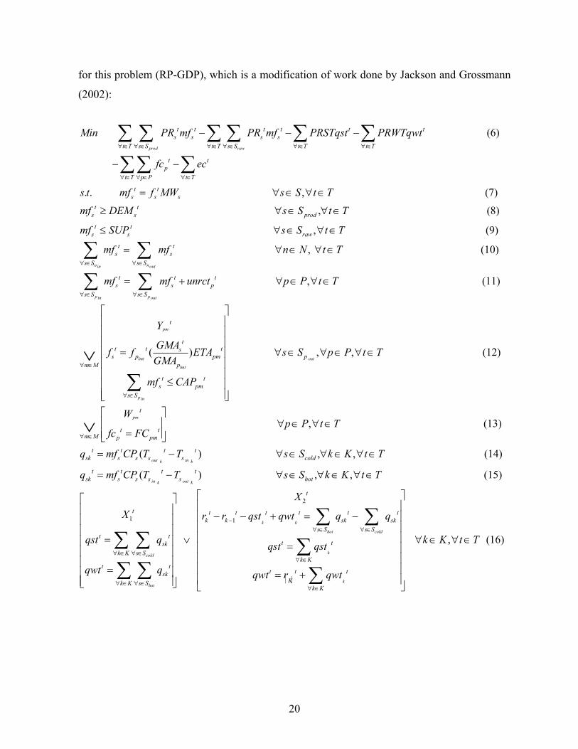
We use a one year planning horizon of four time periods each consisting of 3 months.

Modifications for increased conversion and capacity only are considered, and black-box

(input/output) models are used for each process. We do not include explicit data for this

problem because of its size. The problem was transformed into an MIP model by using both

the big-M and convex hull reformulations given in Appendix C. Problem sizes for both

reformulations are listed in Table 8, while the graphical solution to this problem is presented in

Figure 8.

Table 8. Problem sizes for 10-process retrofit planning problem Total number of constraints Total number of variables Number of discrete variables

Convex Hull 2505 1417 320 Big-M 1957 697 320

Figure 8. Graphical solution for 10-process retrofit planning problem.

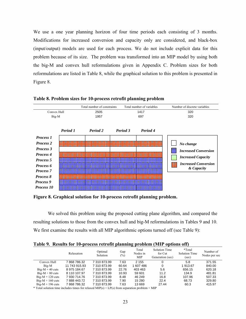
We solved this problem using the proposed cutting plane algorithm, and compared the

resulting solutions to those from the convex hull and big-M reformulations in Tables 9 and 10.

We first examine the results with all MIP algorithmic options turned off (see Table 9):

Table 9. Results for 10-process retrofit planning problem (MIP options off)


Gap (%)

Total Nodes in

MIP


Generation (sec)


(sec)


Convex Hull 7 868 786.32 7 310 873.99 7.63 2 155 0 5.8 371.55 Big-M 11 743 915.93 7 310 873.99 60.64 1 607 486 0 1 913.67 840.00

Big-M + 40 cuts 8 975 184.67 7 310 873.99 22.76 403 463 5.6 656.15 620.18 Big-M + 80 cuts 8 110 107.97 7 310 873.99 10.93 59 601 11.2 134.9 481.81

Big-M + 120 cuts 7 930 714.76 7 310 873.99 8.48 46 249 16.8 107.96 507.33 Big-M + 160 cuts 7 888 443.72 7 310 873.99 7.90 15 280 22.4 68.73 329.80 Big-M + 196 cuts 7 868 786.32 7 310 873.99 7.63 13 669 27.44 60.3 415.97


No change

Increased Conversion Increased Capacity

Increased Conversion & Capacity

Process 1 Process 2 Process 3 Process 4 Process 5 Process 6 Process 7 Process 8 Process 9 Process 10

Period 1 Period 2 Period 3 Period 4

24

The optimal solution of the problem is $7 868 786.32. The upper bound obtained from

the relaxation is equal to $11 743 915.93 for the (BM) reformulation and $7 868 786.32 for the

(CH) reformulation, and the problem was solved in 1 607 486 nodes using the (BM)

reformulation, as opposed to the (CH) reformulation, which required only 2 155 nodes.

Clearly, the (CH) feasible region is tighter than that of the big-M, which results in large

savings in computational time (5.8 sec vs. 1 913.67 sec). After the addition of 40 cutting

planes to the (BM) reformulation, we are able to reduce the relaxation gap by nearly 40% and

solve the problem in 656.15 sec while examining 403 463 nodes in the B&B tree. Upon the

successive addition of more cuts, the number of nodes examined is further reduced, which

results in a further decrease in total solution time. Finally, 196 cuts were generated from the

proposed cutting plane algorithm (requiring 27.44 sec) and the problem was solved to

optimality in a total of 60.3 sec while examining only 13 669 nodes. Furthermore, upon the

addition of all cuts generated, the relaxation gap was reduced to 7.63%, identical to that of the

(CH) relaxation. Although this demonstrates the efficiency of the cuts, and allows the problem

to be solved in much less time than without cuts (60.3 sec vs. 1 913.67 sec), the solution time

required by the (CH) reformulation is less still (5.8 sec). This is due to the extremely tight

region generated by the (CH) reformulation which justifies the additional variables incurred by

the reformulation and allows the problem to be solved in faster times than our method. This

leads us to believe that classes of problems with extremely tight (CH) reformulations are

solved more efficiently as (CH) MIPs through traditional B&B solvers without requiring the

additional cut generation technique that we have developed. On the other hand, the example

shows very good improvement of the big-M formulation with the addition of cutting planes.

The results when default MIP options are turned on present similar trends as previously

discussed and are shown in Table 10.

Table 10. Results for 10-process retrofit planning problem (default options on)


Gap (%)

Total Nodes in

MIP


Generation (sec)


(sec)


Convex Hull 7 868 786.32 7 310 873.99 7.63 35 0 0.578 60.55 Big-M 11 743 915.93 7 310 873.99 60.64 400 612 0 518.64 772.42

Big-M + 40 cuts 8 975 184.67 7 310 873.99 22.76 326 864 5.6 591.4 557.97 Big-M + 80 cuts 8 110 107.97 7 310 873.99 10.93 37 464 11.2 95.04 446.85

Big-M + 120 cuts 7 930 714.76 7 310 873.99 8.48 7 695 16.8 38.41 356.08 Big-M + 160 cuts 7 888 443.72 7 310 873.99 7.9 3 391 22.4 33.6 302.76 Big-M + 196 cuts 7 868 786.32 7 310 873.99 7.63 1 857 27.44 35.89 219.76


25

4.3 Zero-Wait Job Shop Scheduling Problem Consider a job shop scheduling problem where a set of jobs i I∈ must be processed sequentially on a set of consecutive stages j J∈ , where all jobs can be sequenced on a subset of stages ( )j J i∈ . Furthermore, zero-wait transfer is assumed between stages, and the objective is to obtain a schedule that minimizes the makespan ms. The following model (JS-GDP) from Raman and Grossmann (1994) is proposed:

( )

(27)

. . i ijj J i

Min ms

s t ms t TAU∀ ∈

≥ + ∑1 2

( ) ( ) ( ) ( )

(28)

ik ik

i im k km k km i imm J i m J k m J k m J i

m j m j m j m j

i I

Y Y

t TAU t TAU t TAU t TAU∀ ∈ ∀ ∈ ∀ ∈ ∀ ∈

≤ < ≤ <

∀ ∈

⎡ ⎤ ⎡ ⎤⎢ ⎥ ⎢ ⎥

∨+ ≤ + + ≤ +⎢ ⎥ ⎢ ⎥⎢ ⎥ ⎢ ⎥⎣ ⎦ ⎣ ⎦

∑ ∑ ∑ ∑

1 1 2

, , , (29)

, , , , , , ik

i ik ik

j C i k I i k

ms t Y Y True False i k I i k+

∀ ∈ ∀ ∈ <

∈ ∈ ∀ ∈ <R Equations (27) and (28) correspond to the objective function and aim to minimize the makespan ms, where ti is the start time of job i and ijTAU is the processing time of job i in

stage j. Equation (29) ensures that no clash between jobs occurs at any stage at the same time, where for each pair of jobs i,k, the stages with potential clashes are ( ) ( )ikC J i J k= ∩ .

We consider an instance of the zero-wait job-shop scheduling problem with 9 jobs and

8 stages. We do not include explicit data for this problem because of its size. The problem was

transformed into an MIP model by using both the big-M and convex hull reformulations given

in Appendix D. The problem sizes for both reformulations are presented in Table 11, while the

graphical solution to this problem is presented in Figure 9.

Table 11. Problem sizes for 9-job / 8-stage zero-wait job-shop scheduling problem Total number of constraints Total number of variables Number of discrete variables

Convex Hull 681 226 72 Big-M 465 82 72

26

Figure 9. Graphical solution for 9-job / 8-stage zero-wait job-shop scheduling problem

The problem was solved with the proposed cutting plane algorithm and compared with

the results from the convex hull and big-M reformulations in Tables 12 and 13. We first

examine the results with all MIP algorithmic options turned off (see Table 12):

Table 12. Results for 10 job / 8 stage job shop scheduling problem (MIP options off)


Gap (%)

Total Nodes in MIP


Generation (sec)


(sec)


Convex Hull 35.25 66 46.59 27 402 0 12.03 2277.81 Big-M 33 66 50.0 37 260 0 7.47 4987.95

Big-M + 10 cuts 35.25 66 46.59 45 970 0.46 10.43 4610.83 Big-M + 20 cuts 35.25 66 46.59 38 153 0.92 9.17 4624.61 Big-M + 30 cuts 35.25 66 46.59 25 547 1.38 7.01 4619.7


The optimal solution of the problem is 66. The lower bound obtained from the

relaxation is equal to 33 for the (BM) reformulation and 35.25 for the (CH) reformulation, and

the problem was solved in 37 260 nodes using the (BM) reformulation, as opposed to the (CH)

reformulation, which required 27 402 nodes. It is clear that the (CH) feasible region is not

much tighter than that of the (BM) as seen from the poor relaxation value and the number of

nodes examined in the B&B tree. This causes the solution time of (CH) to be larger than that

of (BM) due to the greater number of variables and constraints in the formulation (12.03 sec

vs. 7.47 sec). Furthermore, one can conjecture that since the (CH) feasible region is not much

tighter than that of the (BM), the effect that the cuts will have on overall solution times and

number of nodes examined will be minimal. In fact, after the addition of 30 cutting planes to

the (BM) reformulation, we are able to solve the problem in 7.01 sec while examining 25 547

Stage 1 Stage 2 Stage 3 Stage 4 Stage 5 Stage 6 Stage 7 Stage 8

A

A

A

A

A

A

B

B

B

B

B

B

C

C

CC

C

C

C

D

D

D

D

D

D

D

E

E

E

E

E

E

E

F

F

F

F F

F

F

G

G

G

GG

G

G

H

H

H

HH

H

H

H

I

I

I

I

I

I

I

Optimal makespan: 66

27

nodes in the B&B tree, only slight improvements on the results obtained using the (BM)

reformulation. This leads us to believe that classes of problems with extremely loose (CH)

reformulations are solved efficiently enough as (BM) MIPs through traditional B&B solvers.

The proposed cutting plane algorithm does not improve solution times for this class of

problems since the amount of time required to generate the cuts does not justify the (loose)

tightening the cuts provide. The results when default MIP options are turned on present similar

trends as previously discussed and are shown in Table 13 (note once again, as in the case of

the strip-packing problem, the poor results obtained using the (CH) reformulation).

Table 13. Results for 10 job / 8 stage job shop scheduling problem (default options on)


Gap (%)

Total Nodes in MIP


Generation (sec)


(sec)


Convex Hull 35.25 66 46.59 58 599 0 38.34 1528.4 Big-M 33 66 50.0 9 757 0 1.75 5 575.43

Big-M + 10 cuts 35.25 66 46.59 10 900 0.46 2.55 5 207.84 Big-M + 20 cuts 35.25 66 46.59 6 040 0.92 2.05 5 368.88 Big-M + 30 cuts 35.25 66 46.59 5 562 1.38 2.44 5 247.17


5. CONCLUSION

We have presented in this paper a cutting plane method that adds cuts generated from a

separation problem to a big-M reformulation of a linear GDP problem. We have rigorously

derived the cuts, and applied the method to the strip-packing, retrofit planning and zero-wait

job shop scheduling problems. The results demonstrate the efficiency of the proposed method

for a class of problems where the convex hull relaxation is tighter than that of the big-M, but

not tight enough to justify the additional variables required by the (CH) reformulation. An

example within that class is the strip-packing problem where excellent results were obtained.

Furthermore, we have also highlighted some of the drawbacks of the method regarding other

classes of problems which include the retrofit planning and zero-wait job shop scheduling

problems, where the convex hull relaxation was either too tight or too loose respectively.

We intend to examine in the future different methods that could improve the algorithm,

specifically as pertaining to the judicious selection of those Lagrange multipliers (for the

infinity norm) that generate the “best” cuts for our specific problem. We also intend to

compare the proposed cuts, both theoretically and computationally, to those already present in

the literature and to extend the work to solution methods for convex non-linear GDP problems.

28

ACKNOWLEDGEMENT

The authors would like to gratefully acknowledge financial support from the National Science

Foundation under Grant ACI-0121497.

Literature Cited

Balas E., “Disjunctive Programming: Properties of the convex hull of feasible points”, Invited paper in Discrete Applied Mathematics, 89, 1-44, 1998. Balas E., Ceria S., Cornuejols G., “A lift-and-project cutting plane algorithm for mixed 0-1 programs”, Mathematical Programming, 58 (3), 295-324, 1993. Bazarra M.S., Shetty C.M., “Non-linear programming: theory and algorithms”, Wiley, 1979. Biegler L., Grossmann I.E, Westerberg A. W., “Systematic methods of chemical process design”, Prentice Hall, 1997. Brooke A., Kendrick D., Meeruas A., Raman R., “GAMS language guide”, Version 98, GAMS Development Corporation. Ceria S., Soares J., “Convex programming for disjunctive optimization”, Mathematical Programming, 86 (3), 595-614, 1999. Fletcher R., “Practical methods of optimization”, 2nd edition, John Wiley & Sons, 1987. Grossmann, I.E., A.W. Westerberg and L.T. Biegler, "Retrofit Design of Chemical Processes," Proceedings of Foundations of Computer Aided Process Operations (Eds. G.V. Reklaitis and H.D. Spriggs, Elsevier), 403 (1987). Grossmann I.E., “Review of non-linear mixed-integer and disjunctive programming techniques”, Optimization and Engineering, 3, 227-252, 2002. Grossmann, I.E. and Lee S., “Generalized Disjunctive Programming: Nonlinear Convex Hull Relaxation and Algorithms“, Computational Optimization and Applications, 26, 83-100(2003). Hifi M., “Exact algorithms for the guillotine strip cutting/packing problem”, Computers and Operations Research 25 (11), 925-940, 1998. Hooker J., “Logic-based methods for optimization: combining optimization and constraint satisfaction”, John Wiley & Sons, 2000. Jackson J. and Grossmann I.E., “High-Level optimization model for the retrofit planning of process networks”, Ind. Eng. Chem. Res., 41, 2002, 3762-3770. Lee S. and Grossmann I.E., “New algorithms for nonlinear generalized disjunctive programming”, Computers and Chemical Engineering 24, 2125-2141, 2000.

29

Nemhauser G.L, Wolsey L.A, “Integer and combinatorial optimization”, Wiley Interscience, 1999. Raman R. and Grossmann I.E., “Modeling and computational techniques for logic based integer programming”, Computers and Chemical Engineering 18 (7), 563-578, 1994. Stubbs R. and Mehrotra S., “A Branch-and-Cut Method for 0-1 Mixed Convex Programming”, Mathematical Programming 86, 515-532, 1999. Tawarmalani, M. and N.V. Sahinidis, “Convexification and Global Optimization in Continuous and Mixed-Integer Nonlinear Programming,” Kluwer Academic Publishers, Dordrecht, 2002 Turkay M., Grossmann I.E., “Logic-based MINLP algorithms for the optimal synthesis of process networks”, Computers and Chemical Engineering, 20 (8), 959-978, 1996. Vecchietti, A., S. Lee and I.E. Grossmann, “Modeling of Discrete/Continuous Optimization Problems: Characterization and Formulation of Disjunctions and their Relaxations”, Computers and Chemical Engineering 27, 433-448 (2003). Williams H.P., “Model Building in Mathematical Programming”, Wiley, 1985.

30

APPENDICES

Appendix A. Proofs of Propositions

Proof of Proposition 1:

1) (FR-SEP) ⊆ (FR-BM):

See Grossmann and Lee (2003), Proposition 4.

2)(FRP-SEP) is convex:

From Ceria, Soares (1999) and Grossmann, Lee (2003), we know that (FR-SEP) is a convex

set. Thus, since (FRP-SEP) is the projection of (FR-SEP) from the (z,ν) space onto the z space,

and projection preserves convexity, then (FRP-SEP) is also convex.


1) Let : nφ →R R be defined as || ||bmz z− . Then φ is a convex function for the 1,2 and ∞

norms over all its domain. Also, from Proposition 1, we know that (FRP-SEP) is a convex set.

Furthermore, let ( , )sep sepz ν be the optimal solution of (SEP). Clearly, from the properties of

projection, sepz would be the optimal solution of (SEP1), where (SEP1) is as follows:

(z) || ||. . ( )

bmMin z zs t z FRP SEP

φ = −∈ −

From theorem 3.4.3 in Bazaraa & Shetty (1979), if sepz is an optimal solution to (SEP1), then

φ has a subgradient ξ at sepz such that ( ) 0T sepz zξ − ≥ z∀ ∈(FRP-SEP).

2) From Proposition 1, we know that (FR-SEP) ⊆ (FR-BM). In the case where bmz ∈ (FRP-

SEP), obviously no cut can be generated. Otherwise, bmz ∉ (FRP-SEP) and we show that the

above inequality cuts off bmz . From 1) we know that ( ) 0T sepz zξ − ≥ z∀ ∈(FRP-SEP).

31

Furthermore, ξ is a subgradient of ( )zφ at sepz . By definition of subgradient (Nemhauser &

Wolsey, 1999), for ( )zφ is convex, we have:

( ) ( ) ( ) ( )|| || || || ( ) ( )

, || || || || ( )

( ) || || 0

sep T sep

bm sep bm T sep

bm

bm bm sep bm T bm sep

T bm sep sep bm

z z z z z FRP SEPz z z z z z z FRP SEP

if z z thenz z z z z z

z z z z

φ φ ξ

ξ

ξ

ξ

− ≥ − ∀ ∈ −

⇔ − − − ≥ − ∀ ∈ −

≡

− − − ≥ −

⇔ − ≤ − − <

Thus, bmz does not satisfy ( ) 0T sepz zξ − ≥ and is therefore cut off by the inequality.


If φ is differentiable over S, then φ is differentiable at sepz . It follows from Lemma 3.3.2 in

Bazaraa & Shetty (1979) that the only element of the subdifferential of φ is ( )sepzφ∇ .


If φ is defined as 22( ) || ||bmz z zφ = − , then φ is differentiable and from Proposition 3, the

collection of subgradients of φ at sepz is the singleton set ( )sepzφ∇ . Thus,

( ) ( ) ( ) ( ) 2( )

sep sep bm T sep bm

sep sep bm

z z z z zand z z zφ

φ

= − −

∇ = −

Proof of Proposition 5: Let : Sφ → R be defined as ( ) || ||bmz z zφ ∞= − in (SEP). Then (SEP) can be rewritten as:

. . (A1)

( )

bmi ibm

i i

Min us t u z z i M

u z z i MFR SEP

≥ − ∀ ∈

≥ − ∀ ∈

−

32

From Proposition 1, we know that (FR-SEP) is convex. Furthermore, all the constraints in (FR-SEP) are linear. Thus, (FR-SEP) corresponds to a polytope in the ( , )z ν space, and ∃

matrices 1 2,R R with dimensions ( | |), kk K

m n J m n∈

× × ×∑ respectively and vector mr ∈ R such

that 1 2( ) ( , ) |FR SEP z R z R rν ν− ≡ + ≤ . Note that the non-negativity constraints for z and v

are taken into account in the construction of 1 2,R R . We can thus write (A1) as:

1 2

. . (A2)

bmi ibm

i i

Min us t u z z i M

u z z i M

R z R rν

≥ − ∀ ∈

≥ − ∀ ∈

+ ≤

The appropriate Lagrangian function of (A2) is as follows:

1 2( ) ( ) ( )bm bm Ti i i i i i

i M i M

L u z z u z z u R z R rµ µ ρ ν+ −∈ ∈

= + − − + − − + + −∑ ∑

and it is implied at ( , , )sep sep sepz uν that multipliers sepµ+ , sepµ− and sepρ exist such that:

1

( , , ) 0 1 0 ( ) 1

( , , ) 0 ( ) 0 (A3)

( , , ) 0

sep sep sep

sep

sep sep sepi i i i

i M i M i M

sep sep sep sepTz i i

i Msep sep sep

L z uu

L z u R

L z uν

ν µ µ µ µ

ν µ µ ρ

ν

+ − + −

∈ ∈ ∈

+ −∈

∂= ⇒ − − = ⇒ + =

∂

∇ = ⇒ − + =

∇ = ⇒

∑ ∑ ∑∑

2 0

, , 0 , where | ( ) ( )

sepT

sep sep sep bm bmi i i i i i

R

i M M active M i u z z u z z i M

ρ

µ µ ρ+ −

=

≥ ∀ ∈ ≡ ≡ = − ∨ = − ∀ ∈

Now let us define the following matrix H with columns hi as [ | ]H I I≡ − and the following

vector µ as µ

µµ

+

−

⎡ ⎤≡ ⎢ ⎥

⎣ ⎦.

We claim that if Hξ µ= , then the existence of a vector sep

isep sepsep

i

i Mµµ

µµµ

++

−−

⎡ ⎤ ⎡ ⎤≡ ≡ ∀ ∈⎢ ⎥ ⎢ ⎥

⎢ ⎥ ⎣ ⎦⎣ ⎦ in

(A3) is equivalent to the existence of a vector sepξ in the set:

33

1

2

(A4)

0

00

sep

sep

sep sep sepi

i N

sepTi

i NsepT

sep

conv h

such that

R

R

φ ξ ξ

ξ ρ

ρ

ρ

∈

∈

∂ ≡ ∈

+ =

=

≥

∑

where (A4) is the subdifferential of φ , sepξ is a subgradient of ( )sepzφ and

:| | sep bmi iN i z z is maximized≡ − , according to section 14.1 and Lemma 14.2.2 in Fletcher

(1987). In essence, we are claiming that in order to obtain a subgradient vector sepξ of ( )sepzφ in (A4), one needs only to obtain a set of Lagrange multipliers sepµ from (A3) (thus, the existence of one is equivalent to the existence of the other). We prove the claim as follows: From (A4), we have,

1

2

0

00

with 1, 0

sep

sep

sep sep

sep sep sepi

i N

sepTi

i NsepT

sep

sepi i i i

i N i N

conv h

such that

R

R

h from the convex hull definition

suc

φ ξ ξ

ξ ρ

ρ

ρ

ξ α α α

∈

∈

∈ ∈

∂ ≡ ∈

+ =

=

≥

⇔ = = ≥

∑

∑ ∑

1

2

1

0

00

[ | ] [ ]

1, 0

0

sep

sep

sep

sepTi

i NsepT

sep

sepsep sep sep sep sep sep sep

sep

sepi i

i N

sepTi

i N

h that

R

R

H I I

such that

R

ξ ρ

ρ

ρ

αξ α α α

α

α α α

ξ ρ

∈

++ −

−

+ −∈

∈

+ =

=

≥

⎡ ⎤⇔ = = − = −⎢ ⎥

⎢ ⎥⎣ ⎦

+ = ≥

+ =

∑

∑∑

2

(A5)

00

sepT

sep

Rρ

ρ

=

≥

34

[ | ] [ ]

[ ] [ ]

( 5) [ ], ( 5) :

[ ]

s.t. 1, 0

sep sep sep sepi i i

sep sep sep

sep sep sep

i i ii

If H

I I

Then and i N

but from A we know thatso and A becomes

ξ µµ

ξ µ µµ

ξ µ µ ξ µ µ

ξ α αα µ

ξ µ µ

µ µ µ

++ −

−

+ − + −

+ −

+ −

+ −

=

⎡ ⎤⇔ = − = −⎢ ⎥

⎣ ⎦= − = − ∀ ∈

= −=

= −

+ = ≥

1

2

[ ] 0 (A6)

0 0

sep

sep

N

sepTi i

i NsepT

sep

R

R

µ µ ρ

ρ

ρ

∈

+ −∈

− + =

=

≥

∑∑

Clearly, sep sepN M≡ and we have thus recovered (A3) and shown that the form of the

subgradient is indeed [ ]sep sep sepξ µ µ+ −= − .

35

Appendix B. Reformulations of Strip-Packing Problem (SP-GDP)

a) Big-M reformulation of (SP-GDP):

1 1

2 2

3 3

. .

(1 ) , ,

(1 ) , ,

(1 )

i i

i i j ij ij

j j i ij ij

i i j ij ij

Min lts t lt x L i N

x L x BIGM w i j N i j

x L x BIGM w i j N i j

y H y BIGM w

≥ + ∀ ∈

+ ≤ + − ∀ ∈ <

+ ≤ + − ∀ ∈ <

− ≥ − − ∀4 4

, ,

(1 ) , ,

1 , , ,

j j i ij ij

dij

d D

i i i

i i

i j N i j

y H y BIGM w i j N i j

z d D i j N i j

x UB L i NH y W

∈

∈ <

− ≥ − − ∀ ∈ <

= ∀ ∈ ∀ ∈ <

≤ − ∀ ∈≤ ≤

∑

1

, , , 0,1 , , ,di i ij

i N

lt x y w d D i j N i j+

∀ ∈

∈ ∈ ∀ ∈ ∀ ∈ <R

where D =1,2,3,4. b) Convex Hull reformulation of (SP-GDP):

. .

, , , ,

, ,

i i

dk kij

d D

dk kij

d D

Min lts t lt x L i N

x i j k N i j k i j

y i j k

ν

ω∈

∈

≥ + ∀ ∈

= ∀ ∈ < = ∨

= ∀ ∈

∑∑

1 1 1

2 2 2

3 3 3

4 4

, ,

, ,

, ,

, ,

iij jij i ij

jij iij j ij

iij jij i ij

jij i

N i j k i j

L w i j N i j

L w i j N i j

H w i j N i j

ν ν

ν ν

ω ω

ω ω

< = ∨

− ≤ − ∀ ∈ <

− ≤ − ∀ ∈ <

− ≥ ∀ ∈ <

− 4 , ,

1 , ,

, , , , ,

ij j ij

dij

d Dd d d

kij kij ij

d dkij ki

H w i j N i j

w i j N i j

UB w d D i j k N i j k i j

UB

ν

ω

∈

≥ ∀ ∈ <

= ∀ ∈ <

≤ ∀ ∈ ∀ ∈ < = ∨

≤

∑

1

, , , , ,

, , , , ,

dj ij

i i i

i id d d

i i kij kij i

w d D i j k N i j k i j

x UB L i NH y W i N

lt x y wν ω +

∀ ∈ ∀ ∈ < = ∨

≤ − ∀ ∈≤ ≤ ∀ ∈

∈ R 0,1 , , , , ,j d D i j k N i j k i j∈ ∀ ∈ ∀ ∈ < = ∨

where D =1,2,3,4.

36

Appendix C. Reformulations of Retrofit Planning Problem (RP-GDP)

a) Big-M reformulation of (RP-GDP):

. . ,

prod raw

pm

t t t t t ts s s s


t t tpm j

t T m M p P t T j J

t ts s s

t ts s

Min Z PR mf PR mf PRSTqst PRWTqwt

FC w EFC

s t mf f MW s S t T

mf DEM

∈ ∈ ∈ ∈ ∈ ∈

∈ ∈ ∈ ∈ ∈

= − − −

− −

= ∀ ∈ ∀ ∈

≥

∑ ∑ ∑ ∑ ∑ ∑

∑∑∑ ∑∑

,

,

n nin out

prod

t ts s raw

t ts s

s S s S

s S t T

mf SUP s S t T

mf mf∈ ∈

∀ ∈ ∀ ∈

≤ ∀ ∈ ∀ ∈

=∑ ∑ ,

,

( ) (1 ) , , ,

( ) (1

p pin out

lmt out

lmt

lmt

lmt

t t ts s p

s S s S

tt t t t ts

s p pm pm pm pp

tt t t t ts

s p pm pm pmp

n N t T

mf mf unrct p P t T

GMAf f ETA BIGM y s S p P m M t TGMA

GMAf f ETA BIGM yGMA

∈ ∈

∀ ∈ ∀ ∈

= + ∀ ∈ ∀ ∈

≤ + − ∀ ∈ ∀ ∈ ∀ ∈ ∀ ∈

≥ − −

∑ ∑

) , , ,

(1 ) , ,

(1 ) , ,

(1 )

out

p in

p

t t t ts pm pm pm

s S

t t t tp pm pm pm

t t t tp pm pm pm

s S p P m M t T

mf CAP BIGM y p P m M t T

fc FC BIGM w p P m M t T

fc FC BIGM w p

∈

∀ ∈ ∀ ∈ ∀ ∈ ∀ ∈

≤ + − ∀ ∈ ∀ ∈ ∀ ∈

≤ + − ∀ ∈ ∀ ∈ ∀ ∈

≥ − − ∀

∑

1,1 1

, ,

( ) , ,

( ) , ,

(1 )

out ink k

in outk k

cold


t t t tsk s s s s hot

t t t tsk

k K s S

P m M t T



qst q BIGM x∈ ∈

∈ ∀ ∈ ∀ ∈

= − ∀ ∈ ∀ ∈ ∀ ∈

= − ∀ ∈ ∀ ∈ ∀ ∈

≤ + −∑ ∑1,1 1

2,1 1

2,1 1

1

(1 )

(1 )

(1 )

cold

hot

hot

k

t t t tsk

k K s S

t t t tsk

k K s S

t t t tsk

k K s S

t t tk k

t T

qst q BIGM x t T

qwt q BIGM x t T

qwt q BIGM x t T

r r qst qw

∈ ∈

∈ ∈

∈ ∈

−

∀ ∈

≥ − − ∀ ∈

≤ + − ∀ ∈

≥ − − ∀ ∈

− − +

∑ ∑∑ ∑∑ ∑

1,2 2

1 1,2 2

(1 ) ,

(1 ) ,

k

hot cold

k k

hot cold

t t t t tsk sk

s S s S

t t t t t t t tk k sk sk

s S s S

t q q BIGM x k K t T

r r qst qwt q q BIGM x k K t T

∈ ∈

−∈ ∈

≤ − + − ∀ ∈ ∀ ∈

− − + ≥ − − − ∀ ∈ ∀ ∈

∑ ∑∑ ∑

37

2,2 2

2,2 2

3,2 2

3,2 2

(1 )

(1 )

(1 )

(1 )

k

k

k

k

t t t t

k K

t t t t

k K

t t t t tK

k K

t t t t tK

k K

qst qst BIGM x t T

qst qst BIGM x t T

qwt r qwt BIGM x t T

qwt r qwt BIGM x

∈

∈

∈

∈

≤ + − ∀ ∈

≥ − − ∀ ∈

≤ + + − ∀ ∈

≥ + − −

∑∑

∑∑

(1 ) ,

(1 ) ,

raw

t t t tj j j

t t t tj j j

t t t t t t tp s s

p P s S

pm

t T

ec EFC BIGM v j J t T

ec EFC BIGM v j J t T

fc ec PR mf PRSTqst PRWTqwt INV t T

y

∈ ∈

∀ ∈

≤ + − ∀ ∈ ∀ ∈

≥ − − ∀ ∈ ∀ ∈

+ + + + ≤ ∀ ∈∑ ∑1 ,

1 ,

1

t

m M

tpm

m M

tj

j J

p P t T

w p P t T

x

∈

∈

∈

= ∀ ∈ ∀ ∈

= ∀ ∈ ∀ ∈

=

∑∑∑

1

1

1

, , \

tj

j J

tpm pm

tpm p

t T

v t T

y y p P t T m M m

w w

τ

τ

τ∈

∀ ∈

= ∀ ∈

≤ ∀ ∈ ∀ < ∈ ∀ ∈

≤

∑

1

1 1

1

, , \

,

, ,

t tp p

Tt t t

pm pm pm

p P t T m M m

y w p P t T

y w y p P t Tτ

τ

τ

| |−1−

=

∀ ∈ ∀ ≠ ∈ ∀ ∈

≤ ∀ ∈ ∀ ∈

≤ + ∀ ∈ ∀ ∈∑ 1

2 1

2 1

1 1

\

t

t

t t

m M m

x x t T

v v t T

x v

τ

τ

τ

τ

∀ ∈

≤ ∀ < ∈

≤ ∀ ≠ ∈

≤

2 2 211

,

Tt t t

t ts s

t T

x v x t T

mf f

τ

τ

| |−1−

=

+

∀ ∈

≤ + ∀ ∈

∈

∑R

1

1

1

,

, , ,

, ,

, ,

lmt

t t tp p p

tsk

t t t

s S t T

f unrct fc p P t T

q s S k K t T

qst qwt ec

+

+

+

∀ ∈ ∀ ∈

∈ ∀ ∈ ∀ ∈

∈ ∀ ∈ ∀ ∈ ∀ ∈

∈

R

R

R1

, , ,

, 0,1 , ,

, 0,1

k k

pm pm

t t tk

t t

t tj j

t T

qst qwt r k K t T

y w p P t T m M

x v

+

∀ ∈

∈ ∀ ∈ ∀ ∈

∈ ∀ ∈ ∀ ∈ ∀ ∈

∈

R

,j J t T ∀ ∈ ∀ ∈

38

b) Convex Hull reformulation of (RP-GDP):

. . ,

prod raw

pm

t t t t t ts s s s


t t tpm j

t T m M p P t T j J

t ts s s

t ts s

Min Z PR mf PR mf PRSTqst PRWTqwt

FC w EFC

s t mf f MW s S t T

mf DEM

∈ ∈ ∈ ∈ ∈ ∈

∈ ∈ ∈ ∈ ∈

= − − −

− −

= ∀ ∈ ∀ ∈

≥

∑ ∑ ∑ ∑ ∑ ∑

∑∑∑ ∑∑

,

,

n nin out

prod

t ts s raw

t ts s

s S s S

s S t T

mf SUP s S t T

mf mf∈ ∈

∀ ∈ ∀ ∈

≤ ∀ ∈ ∀ ∈

=∑ ∑ ,

,

, ,

p pin out

out

lmt lmt

t t ts s p

s S s S

t ts sm p

m M

t tp p m

m M

n N t T

mf mf unrct p P t T

f zf s S p P t T

f zf

∈ ∈

∈

∈

∀ ∈ ∀ ∈

= + ∀ ∈ ∀ ∈

= ∀ ∈ ∀ ∈ ∀ ∈

=

∑ ∑

∑∑ ,

, ,

,

in

t ts sm p

m M

t tp pm

m M

t tj

j J

p P t T

mf zmf s S p P t T

fc zfc p P t T

qst zqst

∈

∈

∈

∀ ∈ ∀ ∈

= ∀ ∈ ∀ ∈ ∀ ∈

= ∀ ∈ ∀ ∈

=

∑∑∑

, ,

t tj

j J

t tsk skj cold hot

j J

t tk kj

t T

qwt zqwt t T

q zq s S S k K t T

r zr

∈

∈

∀ ∈

= ∀ ∈

= ∀ ∈ ∪ ∀ ∈ ∀ ∈

=

∑∑

,

,

j J

t tk kj

j J

t tk kj

j J

k K t T

qst zqst k K t T

qwt zqwt k

∈

∈

∈

∀ ∈ ∀ ∈

= ∀ ∈ ∀ ∈

= ∀

∑∑∑ ,

( ) , , ,

lmt out

lmt

p in

t tj

j J

tt t ts

sm p m pm pp

t t tsm pm pm

s S

K t T

ec zec t T

GMAzf zf ETA s S p P m M t TGMA

zmf CAP y

∈

∈

∈ ∀ ∈

= ∀ ∈

= ∀ ∈ ∀ ∈ ∀ ∈ ∀ ∈

≤

∑

∑ , ,

, ,

( ) , ,

(out ink k

in outk

t t tpm pm pm


t t tsk s s s s

p P m M t T

zfc FC w p P m M t T


q mf CP T T

∀ ∈ ∀ ∈ ∀ ∈

= ∀ ∈ ∀ ∈ ∀ ∈

= − ∀ ∈ ∀ ∈ ∀ ∈

= − ) , ,k

thots S k K t T∀ ∈ ∀ ∈ ∀ ∈

39

1 1

1 1

2 1,2 2 2 2 2

cold

hot

hot cold

t tsk

k K s S

t tsk

k K s S

t t t t t tk k k k sk sk

s S s S

zqst zq t T

zqwt zq t T

zr zr zqst zqwt zq zq

∈ ∈

∈ ∈

−∈ ∈

= ∀ ∈

= ∀ ∈

− − + = −

∑ ∑∑ ∑

∑ ∑2 2

2 22

,

t tk

k K

t t tkK

k Kt t t

j j j

k K t T

zqst zqst t T

zqwt zr zqwt t T

zec EFC v

∈

∈

∀ ∈ ∀ ∈

= ∀ ∈

= + ∀ ∈

=

∑∑

,

, , ,

raw

out

lmt lmt

t t t t t t tp s s

p P s S

t t tsm sm pm p

t t tp m p m pm

j J t T

fc ec PR mf PRSTqst PRWTqwt INV t T

zf BND y s S p P m M t T

zf BND y

∈ ∈

∀ ∈ ∀ ∈

+ + + + ≤ ∀ ∈

≤ ∀ ∈ ∀ ∈ ∀ ∈ ∀ ∈

≤

∑ ∑

, ,

, , ,

, ,

in

t t tsm sm pm p

t t tpm pm pm

t t tj j j

p P m M t T

zmf BND y s S p P m M t T

zfc BND w p P m M t T

zqst BND x

∀ ∈ ∀ ∈ ∀ ∈

≤ ∀ ∈ ∀ ∈ ∀ ∈ ∀ ∈

≤ ∀ ∈ ∀ ∈ ∀ ∈

≤ ,

,

t t tj j j

t t tskj skj j

j J t T

zqwt BND x j J t T t T

zq BND x

∀ ∈ ∀ ∈

≤ ∀ ∈ ∀ ∈ ∀ ∈

≤ , , ,

, ,

, ,

cold hot

t t tkj kj j

t t tkj kj j

s S S k K j J t T

zr BND x k K j J t T

zqst BND x k K j J t

∀ ∈ ∪ ∀ ∈ ∀ ∈ ∀ ∈

≤ ∀ ∈ ∀ ∈ ∀ ∈

≤ ∀ ∈ ∀ ∈ ∀ ∈

, ,

,

1

t t tkj kj j

t t tj j j

tpm

m M

T

zqwt BND x k K j J t T

zec BND v j J t T

y∈

≤ ∀ ∈ ∀ ∈ ∀ ∈

≤ ∀ ∈ ∀ ∈

=∑ ,

1 ,

1

1

tpm

m M

tj

j J

tj

j J

p P t T

w p P t T

x t T

v

∈

∈

∈

∀ ∈ ∀ ∈

= ∀ ∈ ∀ ∈

= ∀ ∈

=

∑∑∑

1

1 1

, , \

, , \

tpm pm

tpm p

t T

y y p P t T m M m

w w p P t T m M m

τ

τ

τ

τ

∀ ∈

≤ ∀ ∈ ∀ < ∈ ∀ ∈

≤ ∀ ∈ ∀ ≠ ∈ ∀ ∈

40

1 1

11

2 1

,

, , \

t tp p

Tt t t

pm pm pm

t

y w p P t T

y w y p P t T m M m

x x

τ

τ

τ

| |−1−

=

≤ ∀ ∈ ∀ ∈

≤ + ∀ ∈ ∀ ∈ ∀ ∈

≤

∑

2 1

1 1

2 2 21

t

t t

Tt t t

t T

v v t T

x v t T

x v x

τ

τ

τ

τ

τ

| |−−

=

∀ < ∈

≤ ∀ ≠ ∈

≤ ∀ ∈

≤ +

1

1

, ,

, , lmt

t ts s

t t tp p p

t T

mf f s S t T

f unrct fc

1

+

+

∀ ∈

∈ ∀ ∈ ∀ ∈

∈

∑R

R1

1

,

, ,

, ,

, ,

tsk

t t t

t t tk k k

p P t T

q s S k K t T

qst qwt ec t T

qst qwt r

+

+

∀ ∈ ∀ ∈

∈ ∀ ∈ ∀ ∈ ∀ ∈

∈ ∀ ∈

∈

R

R

R1

1

1

,

, , ,

, ,lmt

t tsm sm

t tp m pm

k K t T

zmf zf s S m M t T

zf zfc p P

+

+

+

∀ ∈ ∀ ∈

∈ ∀ ∈ ∀ ∈ ∀ ∈

∈ ∀ ∈ ∀

R

R1

1

1

,

, , ,

, , ,

, ,

tskm

t t tm m m

t t tkm km km

m M t T

zq s S k K m M t T

zqst zqwt zec m M t T

zqst zqwt zr

+

+

+

∈ ∀ ∈

∈ ∀ ∈ ∀ ∈ ∀ ∈ ∀ ∈

∈ ∀ ∈ ∀ ∈

∈

R

R

R , ,

, 0,1 , ,

, 0,1 ,

pm pmt t

t tj j

k K m M t T

y w p P t T m M

x v j J t T

∀ ∈ ∀ ∈ ∀ ∈

∈ ∀ ∈ ∀ ∈ ∀ ∈

∈ ∀ ∈ ∀ ∈

41

Appendix D. Reformulations of Zero-Wait Job Shop Scheduling Problem (JS-GDP) a) Big-M reformulation of (JS-GDP):

( )

1

( ) ( )

( ) (

. .

(1 ) , , ,

i ijj J i

i im k km ik ikm J i m J km j m j

k km i imm J k m J im j

Min ms

s t ms t TAU i I

t TAU t TAU BIGM y j C i k I i k

t TAU t TAU

∈

∈ ∈≤ <

∈ ∈≤

≥ + ∀ ∈

+ ≤ + + − ∀ ∈ ∀ ∈ <

+ ≤ +

∑∑ ∑

∑ 2

)

1

(1 ) , , ,

1 , ,

, , 0,1

ik ik

m j

dik

d Dd

i ik

BIGM y j C i k I i k

y i k I i k

ms t y

<

∈

+

+ − ∀ ∈ ∀ ∈ <

= ∀ ∈ <

∈ ∈

∑

∑R , , ,i k I i k d D ∀ ∈ < ∀ ∈

b) Convex Hull reformulation of (JS-GDP):

( )

1 1

( )

. .

, , , ,

i ijj J i

dn nik

d D

iik kik kmm J km

Min ms

s t ms t TAU i I

t v i k I i k n I n i k

v v TAU

∈

∈

∈<

≥ + ∀ ∈

= ∀ ∈ < ∀ ∈ = ∨

− ≤

∑∑

1

( )

2 2 2

( ) ( )

, , ,

, , ,

im ik ikm J i

j m j

kik iik im km ik ikm J k m J im j m j

d d dnik ik ik

TAU y j C i k I i k

v v TAU TAU y j C i k I i k

v UB y

∈≤

∈ ∈< ≤

⎛ ⎞⎜ ⎟− ∀ ∈ ∀ ∈ <⎜ ⎟⎜ ⎟⎝ ⎠⎛ ⎞⎜ ⎟− ≤ − ∀ ∈ ∀ ∈ <⎜ ⎟⎜ ⎟⎝ ⎠

≤

∑ ∑

∑ ∑

1

, , , ,

1 , ,

, , 0,1 , , ,

dik

d Dd

i ik

i k I i k n I n i k

y i k I i k

ms t y i k I i k d D∈

+

∀ ∈ < ∀ ∈ = ∨

= ∀ ∈ <

∈ ∈ ∀ ∈ < ∀ ∈

∑R

Documents

A Cutting Plane Method for Solving Linear Generalized ...egon.cheme.cmu.edu/Papers/SawayaGrossmann.pdfA Cutting Plane Method for Solving Linear Generalized Disjunctive Programming